Interdependent Defense Games with Applications to Internet Security at the Level of Autonomous Systems

Abstract

We propose interdependent defense (IDD) games, a computational game-theoretic framework to study aspects of the interdependence of risk and security in multi-agent systems under deliberate external attacks. Our model builds upon interdependent security (IDS) games, a model by Heal and Kunreuther that considers the source of the risk to be the result of a fixed randomized-strategy. We adapt IDS games to model the attacker’s deliberate behavior. We define the attacker’s pure-strategy space and utility function and derive appropriate cost functions for the defenders. We provide a complete characterization of mixed-strategy Nash equilibria (MSNE), and design a simple polynomial-time algorithm for computing all of them for an important subclass of IDD games. We also show that an efficient algorithm to determine whether some attacker’s strategy can be a part of an MSNE in an instance of IDD games is unlikely to exist. Yet, we provide a dynamic programming (DP) algorithm to compute an approximate MSNE when the graph/network structure of the game is a directed tree with a single source. We also show that the DP algorithm is a fully polynomial-time approximation scheme. In addition, we propose a generator of random instances of IDD games based on the real-world Internet-derived graph at the level of autonomous systems (≈27 K nodes and ≈100 K edges as measured in March 2010 by the DIMES project). We call such games Internet games. We introduce and empirically evaluate two heuristics from the literature on learning-in-games, best-response gradient dynamics (BRGD) and smooth best-response dynamics (SBRD), to compute an approximate MSNE in IDD games with arbitrary graph structures, such as randomly-generated instances of Internet games. In general, preliminary experiments applying our proposed heuristics are promising. Our experiments show that, while BRGD is a useful technique for the case of Internet games up to certain approximation level, SBRD is more efficient and provides better approximations than BRGD. Finally, we discuss several extensions, future work, and open problems.

1. Introduction

Attacks carried out by hackers and terrorists in recent decades have led to increased efforts by both government and the private sector to create and adopt mechanisms to prevent future attacks. This effort has yielded a more focused research attention to models, computational and otherwise, that facilitate and help to improve (homeland) security for both physical infrastructure and cyberspace. In particular, there has been quite a bit of recent research activity in the general area of game-theoretic models for terrorism settings (see, e.g., Bier and Azaiez [1] and Cárceles-Poveda and Tauman [2]).

Interdependent security (IDS) games are one of the earliest models resulting from a game-theoretic approach to model security in non-cooperative environments composed of free-will self-interested individual decision-makers. Originally introduced and studied by economists Kunreuther and Heal [3], IDS games model general abstract security problems. In those problems, an individual within a population considers whether to voluntarily invest in some protection mechanisms or security against a risk they may face. Individuals do so knowing that the cost-effectiveness of the decision depends on the investment decisions of others in the population. This is because of transfer risks; that is, the “bad event” may be transferable from a compromised individual to another.

In their work, Kunreuther and Heal [3] provided several examples based on their economics, finance, and risk management expertise. We refer the reader to their paper for more detailed descriptions. As a canonical example of the real-world relevance of IDS settings and the applicability of IDS games, Heal and Kunreuther [4] used this model to describe problems such as airline baggage security. In their setting, individual airlines may choose to invest in additional complementary equipment to screen passengers’ bags and check for hazards such as bombs that could cause damage to their passengers, planes, buildings, or even reputations. However, mainly due to the large amount of traffic volume, it is impractical for an airline to go beyond applying security checks to bags incoming from passengers and include checks to baggage or cargo transferred from other airlines. On the other hand, if an airline invests in security, they can still experience a bad event if the bag was transferred from an airline that does not screen incoming bags, rendering their investment useless. 1 Thus, we can see how the cost-effectiveness of an investment can be highly dependent on others’ investment decisions. Another recent application of the IDS model is on container shipping transportation [6], in which the objective is to study the effect that investment decisions about container screening on some ports may have on neighboring ports.

Some security-related problems in cyberspace are similar, but slightly different in nature to the airline scenario just described. Consider a network where all computers fully trust all other computers and freely exchange information. Each user has complete control over his own computer and can decide if he wants to protect the individual user’s computer from hackers, by installing a firewall, for example. However, that individual user cannot directly control or impose others in the network to protect themselves too. Thus, in order for an individual to feel secure about storing his information on the network, that individual user not only has to think about the security of his own computer, but also the security of other computers on the internal network. This is because any other computer may access that individual user’s computer as well. If any computer were hacked, that individual user’s information would potentially be exposed to the outside world.

Two potential outcomes immediately arise out of the cyber-security scenario. If one does not think enough people have invested in security, then one will not invest either, because any investment will contribute negligibly to the overall protection of one’s data. Also, and this is the aspect that perhaps differentiates cyberspace from the airline security scenario, if nearly everyone has invested in security, one may no longer feel the need to protect oneself. This is because the network is already mostly secure and the amount of work required to protect oneself outweighs the minimal change in overall security. Thus, as many invest, fewer may want to invest.

In this work, we build on the literature in IDS games. In particular, we adapt the model to situations in which the abstract “bad event” results from the deliberate action of an attacker. The “internal agents” (e.g., airlines and computer network users or administrators), whom we also often refer to as “defenders” or “sites,” have the voluntary choice to individually invest in security to defend themselves against a direct or indirect offensive attack, modulo, of course, the cost-effectiveness to do so. As a result, we formally define a new model class: interdependent defense (IDD) games.

In our model, both the attacker(s) 2 and the defenders, modeled as players in a game, make decisions based on cost-benefit analysis. The attacker wants to find the most cost-effective way to attack nodes in the network, and does so by maximizing explicit personal preferences. Similarly, each defender (node in a network) takes into account the costs, as well as potential losses, risks, and actions not only of the attacker, but also of other nodes in the network, when making security investment decisions.

A side benefit of explicitly modeling the attacker, as we do in our model, is that the probability of an attack results directly from the equilibrium analysis. Building IDS games can be hard because it requires a priori knowledge of the likelihood of an attack. Attacks of this kind are considered rare events and thus notoriously difficult to statistically estimate in general.

1.1. Related Work

Johnson et al. [7] and Fultz and Grossklags [8] independently developed non-cooperative game models similar to ours. Johnson et al. [7] extend IDS games by modeling uncertainty about the source of the risk (i.e., the attacker) using a Bayesian game over risk parameters. Fultz and Grossklags [8] propose and study a non-graphical game-theoretic model for the interactions between attackers and nodes in a network. In their model, each node in the network can decide whether to contribute (by investment) to the overall safety of the network or to individual safety. The attackers can attack any number of nodes, but with each attack there is an increased probability that the attacker might get caught and suffer penalties or fines. Hence, while their game has IDS characteristics, it is technically not within the standard IDS game framework introduced by Heal and Kunreuther.

Most of the previous related work explores the realm of information security and is application/network specific (see Roy et al. [9] for a survey on game theory application to network security). Syverson and Systems [10] suggest the use of game-theoretic models (non-cooperative or cooperative) to model the relationship between the attacker and the nodes in the network. Past literature has largely focused on two-person (an attacker and a defender) games where the nodes in the network are regarded as a single entity (or a central defender). For example, Lye and Wing [11] look at the interactions between an attacker and the (system) administrator using a two-player stochastic game. Recent work uses a Stackelberg game model in which the defender (or leader) commits to a mixed strategy to allocate resources to defend a set of nodes in the network, and the follower (or attacker) optimally allocates resources to attack a set of “targets” in the network given the leader’s commitment [12,13,14,15,16].

Very recent work by Smith et al. [17] and Lou and Vorobeychik [18] extends the traditional Stackelberg settings to multiple leaders and use different equilibrium concepts than MSNE. Laszka et al. [19] have used their model to study the interaction among an attacker and multiple defenders in spear-phishing attack settings. The main distinctions of their work to ours are that the defenders are not interconnected, the attacker has some fixed number of attacks (more than one), and the equilibrium concepts studied are different.

Other work strives to understand the motivation of the attackers. For example, Liu [20] focuses on understanding the attacker’s intent, objectives, and strategies, and derive a (two-player) game-theoretic model based on those factors. As another example, Cremonini and Nizovtsev [21] use cost-benefit analysis (of attackers) to address the issue of the optimal amount of security (of the nodes in the network).

1.2. Brief Overview of the Article and the Significance of Our Contributions

We adapt the standard non-cooperative framework of IDS games, which we present and briefly discuss in Section 2, to settings in which the source of the risk is the result of a deliberate, strategic decision by an external attacker. In particular, we design and propose interdependent defense (IDD) games, a new class of games that, in contrast to standard IDS games, model the attacker explicitly, while maintaining a core component of IDS systems: the potential transferability of the risk resulting from an attack. We note that the explicit modeling of risk transfer is an aspect of our model that has not been a focus of previous game-theoretic attacker-defender models of security discussed earlier in Section 1.1.

We formally define and study IDD games in depth in Section 3. There, we also present some characterizations of their MSNE which have immediate computational and algorithmic implications.

In Section 4, we study several computational questions about IDD games. We first provide a polynomial-time algorithm to compute all MSNE for an important subclass of IDD games in Section 3.4. In that subclass, there is only one attack, the defender nodes are fully transfer-vulnerable (i.e., investing in security does nothing to reduce their external/transfer risk), and transfers are one-hop. 3 We describe this subclass in more detail in Section 3.4.

Before continuing, we would like to address two aspects of IDD games brought up in the last paragraph. Note that considering a single attacker is a typical assumption in security settings (see previous work discussed earlier in Section 1.1). It is also reasonable because we can view many attackers as a single attacker. Allowing at most one attack prevents immediate representational and computational intractability problems because, as we state at the beginning of Section 3.2, the number of the attacker’s pure strategies grows exponentially with the number of attacks. Finally, because the attacker has no fixed target, it seems practically ineffective for the attacker to consider or go beyond plans of attacks involving multiple (>2) transfers: such plans are complex, time consuming, and costly. Having said that, there has been increased interest over the last few years in the network security community to explicitly model multiple attackers [22]. For instance, Merlevede and Holvoet [22] view the multi-attacker setting as a very important future direction. Here, we focus most of our technical results and experiments to the single-attacker setting. Yet, we present multi-attacker extensions of our proposed model in Appendix E, where we also discuss some ideas and very preliminary technical results for the multi-attacker setting.

In Section 4.2, we formally prove that our results for computing all MSNE in a subclass of IDS games in polynomial time is unlikely to extend to arbitrary IDD games. Given that, we move on to explore approximate MSNE in IDD games in Section 4.3 and provide a fully polynomial-time approximation scheme (FPTAS) for the case in which the graph over the sites is a directed tree-like network. We note that the attacker is still connected to every site in the network. To place the significance of this result in context, we note that despite the apparent simplicity of the subgraph over the sites, there may be very important real-world applications in supply chains (e.g., see [23]) and the power grid [24], for example.

Our computational results in Section 4 are significant, and some initially surprising to us, within the context of the state of the art in computational and algorithmic game theory. Computing all MSNE in graphical IDS games is hard in general. For instance, the so-called Nash-extension computational problem in general IDS games is NP-complete [25]. To place our computational contributions in an even broader context, note that deciding whether an arbitrary graphical game has a pure-strategy Nash equilibrium (PSNE) is in general NP-complete [26]. In addition, many problems related to computing MSNE with particular properties, even in normal-form games, are NP-complete [27]. Indeed, computing an MSNE is PPAD-complete, even in two-player games [28], thus considered computationally intractable in general. Some alternative proofs of PPAD-completeness for two-player games are polynomial time reductions from graphical games, even if each player in the graphical game has at most 3 players [29]. We refer the reader to Papadimitriou [30] for more information on the complexity class PPAD and to Daskalakis et al. [31] for high-level information about the most recent computational results on the complexity of computing MSNE in normal-form games, and indirectly graphical games too. Also, computing all MSNE is rarely achieved and counting-related problems are often #P-complete. We refer the reader to, for example, Conitzer and Sandholm [32], and the references therein, for additional information. We do not know of any other non-trivial game for which there exists a polynomial-time algorithm to compute all MSNE except the one we provide in Section 4.1 here and the algorithm for uniform-transfer IDS games of Kearns and Ortiz [25]. Finally, while our hardness results build on those for graphical IDS games [25], there does not exist any analogous to our FPTAS for graphical IDS games. It seems that an FPTAS in the IDS setting may be possible by modifying the one we design here, and its proof, to that setting.

We provide experimental results in Section 5. In our experiments, we study the application of learning-in-games heuristics to compute approximate MSNE to both fixed and randomly-generated instances of IDD games. We focus on the class of games with at most one simultaneous attack and one-hop transfers. Our particular object of study is a very large Internet-derived graph at the level of autonomous systems (AS) (≈27 K nodes and ≈100 K edges) obtained from DIMES [33,34] for March 2010, the last network graph available to us. Cybersecurity scenarios motivate this study. We refer the reader to Roy et al. [9] for some examples. Here, we propose a generative model of single-attack IDD games based on the aforementioned Internet graph. For simplicity, we refer to the models that a simulator that we built based on the generative model outputs as Internet games (IGs). In our experiments, we employ simple best-response heuristics from learning in games [35] to compute (approximate) MSNE in IGs. In particular, we perform a series of experiments to both show the large-scale feasibility and scalability of the model and approach. We also explore the behavior of the internal players and the attacker in the resulting equilibria, and the properties of the network-structure induced at an equilibrium.

In Section 6, we provide a discussion of future work, some open problems, and a summary of our contributions.

2. Interdependent Security Games, and a Generalization

Each player i in a finite set $\left[n\right]\equiv \{1,2\dots ,n\}$ of n players of an IDS game has a binary choice, to invest ($a_i=1$) or not to invest ($a_i=0$) in security mechanisms to protect themselves from a potential bad event. For each player i, the parameters $C_i$ and $L_i$ correspond to the cost of investment and loss induced by the bad event, respectively. We define the ratio of the two parameters, the player’s “cost-to-loss” ratio, as $R_i\equiv C_i/L_i$. Bad events can occur through both direct and indirect means. The direct risk, or internal risk, parameter $p_i$, is the probability that player i will experience a bad event because of direct contamination. The standard IDS model assumes that investing will completely protect the player from direct contamination; hence, internal risk is only possible when $a_i=0$. The indirect-risk parameter $q_{ji}$ is the probability that player j is directly “contaminated,” does not experience the bad event, but transfers it to player i who ends up experiencing the bad event. This discussion leads us to the following definition of standard IDS games.

Definition 1.

(Standard IDS Games) An IDS game is defined by a tuple $(n,\mathbf{C},\mathbf{L},\mathbf{p},\mathbf{Q})$, where $\mathbf{C}\equiv {\left(C_i\right)}_{i\in \left[n\right]}$, $\mathbf{L}\equiv {\left(L_i\right)}_{i\in \left[n\right]}$, $\mathbf{p}\equiv {\left(p_i\right)}_{i\in \left[n\right]}$, $\mathbf{Q}$ is a matrix representation of the $q_{ij}$’s, where $(i,j)\in {\left[n\right]}^2$. Implicit in Definition 1 is that $q_{ii}=0$ for all i.

Before we provide a formal definition of the model semantics in the upcoming paragraphs in this section, as a preview, we want to highlight that the standard IDS model assumes that the interactions between players are unaffected by investment in security. Said differently, each individual player’s transferred risk is the same regardless of whether the player invests in security, or not.

We now formally define a (directed) graphical-games [36,37] version of IDS games, as first introduced by Kearns and Ortiz [25]. The reason we introduce graphical IDS games here is to emphasize that the matrix $\mathbf{Q}$ is often sparse and their non-zero entries lead to a network structure captured by an induced graph $G=\left(\right[n],E)$. That way the representation size of a graphical IDS game is not $n^2$, as in standard IDS games, but essentially the number of directed edges E of G, which could potentially be significantly smaller than $n^2$. In addition, we can exploit the sparse representation and the network structure to provide provably tractable computational solutions in some cases.

Definition 2.

(Graphical IDS Games) The parameters $q_{ij}$’s induce a directed graph $G=\left(\right[n],E)$ such that $E\equiv \left\{(i,j)\right|q_{ij}>0\}$. Indeed, we assume that $\mathbf{Q}$ has a sparse-matrix representation as a list of non-zero $q_{ij}$ values for each edge $(i,j)\in E$. Thus, the representation size of $\mathbf{Q}$ is $O\left(\right|E\left|\right)$. Agraphical IDS game is defined by the tuple $(n,G,\mathbf{C},\mathbf{L},\mathbf{p},\mathbf{Q})$.

We now discuss the game-theoretic semantics of (graphical) IDS games. For each player $i\in \left[n\right]$, let $\mathrm{Pa}\left(i\right)\equiv \{j\in \left[n\right]\mid q_{ji}>0\}$ be the set of players that are parents of player i in G (i.e., the set of players that player i is exposed to via transfers); and $\mathrm{PF}\left(i\right)\equiv \mathrm{Pa}\left(i\right)\cup \left\{i\right\}$ be the parent family of player i, which includes i. Denote by $k_i\equiv \left|\mathrm{PF}\left(i\right)\right|$ the size of the parent family of player i. Similarly, let $\mathrm{Ch}\left(i\right)\equiv \{j\in \left[n\right]\mid q_{ij}>0\}$ be the set of players that are children of player i (i.e., the set of players to whom player i can present a risk via transfer) and $\mathrm{CF}\left(i\right)\equiv \mathrm{Ch}\left(i\right)\cup \left\{i\right\}$ the (children) family of player i, which includes i. The probability that player i is safe from player j, as a function of player j’s decision, is

$$e_{ij}\left(a_j\right)\equiv a_j+(1-a_j)(1-q_{ji})={(1-q_{ji})}^{1-a_j}.$$

(1)

Equation (1) results from noting that if j invests, then it is impossible for j to transfer the bad event, while if j does not invest, then j either experiences the bad event or transfers it to another player, but never both. 4 The player receiving the transfer still has the chance of not experiencing the bad event. However, without some form of screening of transfers, this chance is usually very low.

Denote by $\mathbf{a}\equiv (a_1,\dots ,a_n)\in {\{0,1\}}^n$ the joint action of all n players. Also denote by ${\mathbf{a}}_{-i}$ the joint action of all players except i, and for any subset $I\subset \left[n\right]$ of players, denote by ${\mathbf{a}}_I$ the sub-component of the joint action corresponding to those players in I only. We define i’s overall safety from all other players as

$$\begin{array}{c}\hfill s_i\left({\mathbf{a}}_{\mathrm{Pa}\left(i\right)}\right)\equiv {\prod }_{j\in \mathrm{Pa}\left(i\right)}{e}_{ij}\left(a_j\right),\end{array}$$

(2)

and equivalently the overall risk from some other players as

$$\begin{array}{c}\hfill r_i\left({\mathbf{a}}_{\mathrm{Pa}\left(i\right)}\right)\equiv 1-s_i\left({\mathbf{a}}_{\mathrm{Pa}\left(i\right)}\right).\end{array}$$

(3)

Note that, as given in Equation (2) (and Equation (3)), each players’ external safety (and risk) is a direct function of its parents only, not all other players. Note also that from the perspective of each players’ preferences, as quantified by their cost functions presented next (Equation (4)), the source of each player’s transfer risk is independent over the player’s parents in the graph. This independence assumption comes from the original definition of standard IDS games, but there the graph is fully connected (i.e., $\mathrm{Pa}\left(i\right)=\left[n\right]-\left\{i\right\}$) [3]. From these definitions, we obtain player i’s overall cost function: the cost of joint action $\mathbf{a}\in {\{0,1\}}^n$, corresponding to the (binary) investment decision of all players, is

$$\begin{array}{cc}\hfill M_i(a_i,{\mathbf{a}}_{\mathrm{Pa}\left(i\right)})\equiv & a_i[C_i+r_i\left({\mathbf{a}}_{\mathrm{Pa}\left(i\right)}\right)L_i]+(1-a_i)[p_i+(1-p_i)r_i\left({\mathbf{a}}_{\mathrm{Pa}\left(i\right)}\right)]L_i.\hfill \end{array}$$

(4)

Whether players invest depends solely on what they can gain or lose by investing. If the overall cost of investing is less than the overall cost of not investing, the player will invest. Applying this logic to cost function $M_i$ in Equation (4), player i will invest if

$$\begin{array}{c}\hfill C_i+r_i\left({\mathbf{a}}_{\mathrm{Pa}\left(i\right)}\right)L_i<[p_i+(1-p_i)r_i\left({\mathbf{a}}_{\mathrm{Pa}\left(i\right)}\right)]L_i\end{array}$$

(5)

so that the investment cost and the losses due to a transferred event do not outweigh the losses from an internal or transferred bad event. Similarly, if the inequality in the last expression is reversed or is replaced by equality, player i will not invest or would be indifferent, respectively. Rearranging the expression for the best-response condition for strictly playing $a_i=1$, given in the last equation (Equation (5)), and letting ${\Delta }_i\equiv R_i/p_i=\frac{C_i}{p_i{L}_i},$ the cost-to-expected-loss ratio of player i, we get the following best-response correspondence ${\mathcal{BR}}_i:{\{0,1\}}^{k_i-1}\to 2^{\{0,1\}}$ for player i: 5 for all ${\mathbf{a}}_{\mathrm{Pa}\left(i\right)}\in {\{0,1\}}^{k_i-1}$,

$${\mathcal{BR}}_i\left({\mathbf{a}}_{\mathrm{Pa}\left(i\right)}\right)\equiv \left\{\begin{array}{cc}\left\{1\right\},\hfill & \mathrm{if}{s}_i\left({\mathbf{a}}_{\mathrm{Pa}\left(i\right)}\right)>{\Delta }_i,\hfill \\ \left\{0\right\},\hfill & \mathrm{if}{s}_i\left({\mathbf{a}}_{\mathrm{Pa}\left(i\right)}\right)<{\Delta }_i,\hfill \\ \{0,1\},\hfill & \mathrm{if}{s}_i\left({\mathbf{a}}_{\mathrm{Pa}\left(i\right)}\right)={\Delta }_i.\hfill \end{array}\right.$$

(6)

In other words, whether it is cost-effective for player i to invest or not depends on a simple threshold condition on the player’s safety: Does the player feel safe enough from others?

Definition 3.

A joint-action ${\mathbf{a}}^{*}\in {\{0,1\}}^n$ is a pure-strategy Nash equilibrium (PSNE) of a graphical IDS game $(n,G,\mathbf{C},\mathbf{L},\mathbf{p},\mathbf{Q})$ (see Definition 2) if $a_i^{*}\in {\mathcal{BR}}_i\left({\mathbf{a}}_{\mathrm{Pa}\left(i\right)}^{*}\right)$ for all players i (i.e., ${\mathbf{a}}^{*}$ is a mutual best-response, as defined in Equation (6)).

2.1. Generalized IDS Games

In the standard IDS game model, investment in security does not reduce transfer risks. However, in some IDS settings (e.g., vaccination and cyber-security), it is reasonable to expect that security investments would include mechanisms to reduce transfer risks. This motivates our first modification to the traditional IDS games: allowing the investment in protection to not only make us safe from direct attack but also partially reduce (or even eliminate) the transfer risk. Thus, we introduce a new real-valued parameter ${\alpha }_i\in [0,1]$ representing the probability that a transfer of a potentially bad event will go unblocked by i’s security, assuming i has invested. Thus, we redefine player i’s overall cost as 6

$$\begin{array}{c}\hfill M_i(a_i,{\mathbf{a}}_{\mathrm{Pa}\left(i\right)})\equiv a_i[C_i+{\alpha }_i{r}_i\left({\mathbf{a}}_{\mathrm{Pa}\left(i\right)}\right)L_i]+(1-a_i)[p_i+(1-p_i)r_i\left({\mathbf{a}}_{\mathrm{Pa}\left(i\right)}\right)]L_i.\end{array}$$

(7)

We call the generalization α-IDS games, where $\mathit{\alpha }\equiv ({\alpha }_1,{\alpha }_2,\dots ,{\alpha }_n)$ corresponds to the vector composed of the parameter values of each player. This discussion leads to the following definition.

Definition 4.

A graphical α-IDS game, or simply α-IDS game, is given by a tuple $(n,G,\mathbf{C},\mathbf{L},\mathbf{p},\mathbf{Q},\mathit{\alpha })$, where each tuple-entry is as defined in the discussion above, and the semantics of the cost functions $M_i$’s of the players is as defined in Equation (7).

From a game-theoretic perspective, the key aspect of the α parameters is that they determine the characteristics of the best-response behavior of each player. That is, it allows us to model players that may behave in a way that is consistent with behavior that ranges from strategic complementarity (e.g., airline setting, where ${\alpha }_i=1$), all the way to strategic substitutability (e.g., vaccination setting, where ${\alpha }_i=0$), based on the relationship between ${\alpha }_i$ and $1-p_i$.

The corresponding definition of PSNE for α-IDS games is analogous to that given in Definition 3. Hence, we do not formally re-state it here.

3. Interdependent Defense Games

Building from generalized IDS games, in this section we introduce interdependent defense (IDD) games. We begin by introducing an additional player, the attacker, who deliberately initiates bad events: now bad events are no longer “chance occurrences” without any strategic deliberation. 7 The attacker has a target decision for each player - a choice of attack ($b_i=1$) or not attack ($b_i=0$) player i. Hence, the attacker’s pure strategy is denoted by the vector $\mathbf{b}\in {\{0,1\}}^n$. (We discuss an extension of the model to multiple attackers in Appendix E.)

Changing from “random” non-strategic attacks, whose probability of occurrence is determined independent of the actions of the internal players, to intentional attacks, in which actions are deliberately carried out by an external actor, leads us to alter $p_i$ and $q_{ij}$. This is because their original definitions imply extra meaning with respect to the new aggressor.

The game parameter $p_i$ implicitly “encodes” $b_i$ because $b_i=0$ implies $p_i=0$. Thus, we redefine

$$\begin{array}{c}\hfill p_i\equiv p_i\left(b_i\right)\equiv b_i{\widehat{p}}_i\end{array}$$

(8)

so that player i has intrinsic risk ${\widehat{p}}_i$, and only has internal risk if targeted (i.e, $b_i=1$). The new parameter ${\widehat{p}}_i$ represents the (conditional) probability that an attack is successful at site player i given that site i was directly targeted and did not invest in protection.

Similarly, the game parameter $q_{ij}$ “encodes” $b_i=1$, because a prerequisite is that i is targeted before it can transfer the bad event to j. We redefine

$$\begin{array}{c}\hfill q_{ij}\equiv q_{ij}\left(b_i\right)\equiv b_i{\widehat{q}}_{ij}\end{array}$$

(9)

so that ${\widehat{q}}_{ij}$ is the intrinsic transfer probability from player i to player j, independent of $b_i$. The new parameter ${\widehat{q}}_{ij}$ represents the (conditional) probability that an attack is successful at player j given that it originated at player i, did not occur at i, but was transferred undetected to j.

Because the $p_i$’s and $q_{ij}$’s depend on the attacker’s action $\mathbf{b}$, so do the safety and risk functions. In particular, we now have

$$\begin{array}{cc}\hfill e_{ij}(a_j,b_j)\equiv & a_j+(1-a_j)(1-b_j{\widehat{q}}_{ji})={(1-{\widehat{q}}_{ji})}^{b_j(1-a_j)},\mathrm{and}\hfill \end{array}$$

(10)

$$\begin{array}{cc}\hfill s_i({\mathbf{a}}_{\mathrm{Pa}\left(i\right)},{\mathbf{b}}_{\mathrm{Pa}\left(i\right)})\equiv & \prod _{j\in \mathrm{Pa}\left(i\right)}{e}_{ij}(a_j,b_j)\equiv 1-r_i({\mathbf{a}}_{\mathrm{Pa}\left(i\right)},{\mathbf{b}}_{\mathrm{Pa}\left(i\right)}),\hfill \end{array}$$

(11)

where ${\widehat{p}}_i$ and ${\widehat{q}}_{ji}$ are as defined in Equations (8) and (9), respectively. Hence, for each site player i, the cost function becomes

$$\begin{array}{c}\hfill M_i(a_i,{\mathbf{a}}_{\mathrm{Pa}\left(i\right)},b_i,{\mathbf{b}}_{\mathrm{Pa}\left(i\right)})\equiv a_i[C_i+{\alpha }_i{r}_i({\mathbf{a}}_{\mathrm{Pa}\left(i\right)},{\mathbf{b}}_{\mathrm{Pa}\left(i\right)})L_i]+(1-a_i)[b_i{\widehat{p}}_i+(1-b_i{\widehat{p}}_i)r_i({\mathbf{a}}_{\mathrm{Pa}\left(i\right)},{\mathbf{b}}_{\mathrm{Pa}\left(i\right)})]L_i,\end{array}$$

(12)

where ${\widehat{p}}_i$ and $r_i$ are as defined in Equations (8) and (11), respectively. Let

$$\begin{array}{c}\hfill {\widehat{\Delta }}_i\equiv R_i/{\widehat{p}}_i\equiv \frac{C_i}{{\widehat{p}}_i{L}_i}\end{array}$$

(13)

and

$$\begin{array}{c}\hfill {\widehat{s}}_i({\mathbf{a}}_{\mathrm{Pa}\left(i\right)},{\mathbf{b}}_{\mathrm{PF}\left(i\right)})\equiv b_i{s}_i({\mathbf{a}}_{\mathrm{Pa}\left(i\right)},{\mathbf{b}}_{\mathrm{Pa}\left(i\right)})+\frac{1-{\alpha }_i}{{\widehat{p}}_i}{r}_i({\mathbf{a}}_{\mathrm{Pa}\left(i\right)},{\mathbf{b}}_{\mathrm{Pa}\left(i\right)}),\end{array}$$

(14)

where $s_i$ is as defined in Equation (11). The pure-strategy best-response correspondence of each site i is

$$\begin{array}{c}\hfill {\mathcal{BR}}_i({\mathbf{a}}_{\mathrm{Pa}\left(i\right)},{\mathbf{b}}_{\mathrm{PF}\left(i\right)})\equiv \left\{\begin{array}{cc}\left\{1\right\},\hfill & \mathrm{if}{\widehat{s}}_i({\mathbf{a}}_{\mathrm{Pa}\left(i\right)},{\mathbf{b}}_{\mathrm{PF}\left(i\right)})>{\widehat{\Delta }}_i,\hfill \\ \left\{0\right\},\hfill & \mathrm{if}{\widehat{s}}_i({\mathbf{a}}_{\mathrm{Pa}\left(i\right)},{\mathbf{b}}_{\mathrm{PF}\left(i\right)})<{\widehat{\Delta }}_i,\hfill \\ \{0,1\},\hfill & \mathrm{if}{\widehat{s}}_i({\mathbf{a}}_{\mathrm{Pa}\left(i\right)},{\mathbf{b}}_{\mathrm{PF}\left(i\right)})={\widehat{\Delta }}_i,\hfill \end{array}\right.\end{array}$$

(15)

where ${\widehat{\Delta }}_i$ and ${\widehat{s}}_i$ are as defined in Equations (13) and (14), respectively.

We assume that the attacker wants to cause as much damage as possible. Here, we define the utility/payoff function U quantifying the objective of the attacker as

$$\begin{array}{cc}\hfill U(\mathbf{a},\mathbf{b})& \equiv {\sum }_{i=1}^n{M}_i({\mathbf{a}}_{\mathrm{PF}\left(i\right)},{\mathbf{b}}_{\mathrm{PF}\left(i\right)})-a_i{C}_i-b_i{C}_i^0,\hfill \end{array}$$

(16)

where $C_i^0$ is the attacker’s own “cost” to target player i. 8

Of course, many other utility functions of varied complexity are also possible. Indeed, one can consider increasingly complex and sophisticated utility functions that may explicitly parse out the involved costs and induced losses in finer-grain and painstaking detail. For instance, we could decompose the cost to the attacker to target a specific site into different components such as, perhaps, planning and setup costs, carry-out costs, and the costs of getting caught or retaliated against, to name a few. We leave those more complex variants for future work.

Definition 5.

A single-attacker graphical IDD game, or simply IDD game , is given by the tuple $(n,G,\mathbf{C},\mathbf{L},{\mathbf{C}}^0,\widehat{\mathbf{p}},\widehat{\mathbf{Q}},\mathit{\alpha })$, where the tuple’s entries, as well as the model semantics, are as defined in the preceding discussion (Equations (8), (9), (12) and (16)), and the matrix $\widehat{\mathbf{Q}}$ is analogous to the matrix $\mathbf{Q}$ described in Definition 2.

The attacker’s pure-strategy best-response correspondence ${\mathcal{BR}}_0:{\{0,1\}}^n\to 2^{{\{0,1\}}^n}$: 9

$${\mathcal{BR}}_0\left(\mathbf{a}\right)\equiv \underset{\mathbf{b}\in {\{0,1\}}^n}{arg\; max}U(\mathbf{a},\mathbf{b}),$$

(17)

where U is as defined in Equation (16).

Definition 6.

A pure-strategy profile $({\mathbf{a}}^{*},{\mathbf{b}}^{*})\in {\{0,1\}}^{2n}$ is a PSNE of an IDD game if, for each player i, $a_i^{*}\in {\mathcal{BR}}_i({\mathbf{a}}_{\mathrm{Pa}\left(i\right)}^{*},{\mathbf{b}}_{\mathrm{PF}\left(i\right)}^{*})$, and for the attacker, ${\mathbf{b}}^{*}\in {\mathcal{BR}}_0\left({\mathbf{a}}^{*}\right)$, where ${\mathcal{BR}}_i$ and ${\mathcal{BR}}_0$ are as defined in Equations (15) and (17), respectively.

3.1. Conditions on Model Parameters

We now introduce the following reasonable restrictions on the game parameters. We employ these conditions without loss of generality from a mathematical and computational standpoint, as we now discuss.

The first condition states that every site’s investment cost is positive and (strictly) smaller than the conditional expected direct loss if the site were to be attacked directly ($b_i=1$). That is, if a site knows that an attack is directed against it, the site will prefer to invest in security, unless the external risk is too high. This condition is reasonable because otherwise the player will never invest regardless of what other players do (i.e., “not investing” would be a dominant strategy).

Assumption 1.

For all sites $i\in \left[n\right]$, $0<C_i<{\widehat{p}}_i{L}_i$.

The second condition states that, for all sites i, the attacker’s cost to attack i is positive and (strictly) smaller than the expected loss achieved (i.e., gains from the perspective of the attacker) if an attack initiated at site i is successful, either directly at i or at one of its children (after transfer). That is, if an attacker knows that an attack is rewarding (or able to obtain a positive utility), it will prefer to attack some nodes in the network. This assumption is also reasonable; otherwise the attacker will never attack regardless of what other players do (i.e., not attacking would be a dominant strategy, leading to an easy problem to solve).

Assumption 2.

For all sites $i\in \left[n\right]$, $0<C_i^0<{\widehat{p}}_i{L}_i+{\sum }_{j\in \mathrm{Ch}\left(i\right)}{\widehat{q}}_{ij}{\alpha }_j{L}_j$.

In what follows, we study the problem of finding and computing MSNE in IDD games under Assumptions 1 and 2.

3.2. There Is No PSNE in Any IDD Game with at Most One (Simultaneous) Attack

Note that the attacker has in principle an exponential number of pure strategies. For IDD games this translates to a number of simultaneous attacks being $2^n$. This presents several challenges.

One is the question of how one would compactly represent an attacker’s strategy (or policy) over $2^n$ events, when the representation size of the model is $N=O\left(\right|E|+n)$, which is $O\left(n^2\right)$ in the worst case. Thus, one would need a representation of the attacker’s policy that is polynomial in N.

Another related question is how realistic is for the attacker to have such a huge amount of power.

One way to deal with the compact representation, while at the same time realistically constraining the attacker’s power, is to limit the number of simultaneous attack sites to some small finite number $K\ll n$. Even then, the number of pure strategies will grow exponentially in the number of potential attacks K, which still renders the attacker’s pure-strategy space unrealistic, especially on a very large network with about 30 K nodes and 100 K edges, like the one we study in our experiments (Section 5). Worst-case, we need to consider up to $2^n$ number of pure strategies for K attacks as K goes to n. The simplest version of this constraint is to allow at most a single (simultaneous) attack (i.e., $K=1$).

Assumption 3.

The set of pure strategies of the attacker is

$$\mathcal{B}=\left\{\mathbf{b}\in {\{0,1\}}^n\left|{\sum }_{i=1}^n{b}_i\le 1\right.\right\}.$$

We emphasize that Definition 7 does not explicitly preclude multiple attacks, just that they cannot occur simultaneously.

For convenience, we introduce the following definition.

Definition 7.

We say an IDD game is a game with a single simultaneous attack, or simply a single-attack game for brevity, if Assumption 3 holds (i.e., at most one simultaneous attack is possible).

The following technical results on single-attack IDD games will also be convenient.

Lemma 1.

The following holds in any single-attack IDD game $(\left[n\right],G,\mathbf{C},\mathbf{L},\widehat{\mathbf{p}},\widehat{\mathbf{Q}},\mathit{\alpha })$: for all players $i\in \left[n\right]$, for all ${\mathbf{a}}_{\mathrm{Pa}\left(i\right)}$ and ${\mathbf{b}}_{\mathrm{PF}\left(i\right)}$,

$$\begin{array}{cc}\hfill r_i({\mathbf{a}}_{\mathrm{Pa}\left(i\right)},{\mathbf{b}}_{\mathrm{Pa}\left(i\right)})=& \sum _{j\in \mathrm{Pa}\left(i\right)}{b}_j(1-a_j){\widehat{q}}_{ji},s_i({\mathbf{a}}_{\mathrm{Pa}\left(i\right)},{\mathbf{b}}_{\mathrm{Pa}\left(i\right)})=1-r_i({\mathbf{a}}_{\mathrm{Pa}\left(i\right)},{\mathbf{b}}_{\mathrm{Pa}\left(i\right)})\mathit{and}\hfill \end{array}$$

(18)

$$\begin{array}{cc}\hfill b_i{s}_i({\mathbf{a}}_{\mathrm{Pa}\left(i\right)},{\mathbf{b}}_{\mathrm{Pa}\left(i\right)})=& b_i.\hfill \end{array}$$

(19)

The proof is in Appendix B.1.

Proposition 1.

In any single-attack IDD game $(\left[n\right],G,\mathbf{C},\mathbf{L},\widehat{\mathbf{p}},\widehat{\mathbf{Q}},\mathit{\alpha })$, we have that for all players $i\in \left[n\right]$, for all $\mathbf{a}$ and $\mathbf{b}$,

$$\begin{array}{c}\hfill U(\mathbf{a},\mathbf{b})=\sum _{i=1}^n{b}_i{U}_i\left(\mathbf{a}\right),\end{array}$$

(20)

where for all $i=1,\dots ,n$,

$$\begin{array}{c}\hfill U_i\left(\mathbf{a}\right)\equiv (1-a_i)\left({\widehat{p}}_i{L}_i+\sum _{j\in \mathrm{Ch}\left(i\right)}{\widehat{q}}_{ij}(a_j{\alpha }_j+(1-a_j))L_j\right)-C_i^0.\end{array}$$

(21)

The proof is in Appendix B.2.

We note that single-attack IDD games are instances of graphical multi-hypermatrix games [40], in which the local hypergraph of each site $i\in \left[n\right]$ has vertices $\mathrm{PF}\left(i\right)\cup \left\{0\right\}$, where 0 denotes the attacker node, and hyperedges $\{\left\{i\right\},\{0,i\}\}\cup {\bigcup }_{j\in \mathrm{Pa}\left(i\right)}\left\{\{0,i,j\}\right\}$, while the local hypergraph of the attacker has $n+1$ vertices $\left[n\right]\cup \left\{0\right\}$ and hyperedges $\left\{\left\{0\right\}\right\}\cup {\bigcup }_{i\in \left[n\right]}\left(\left\{\{0,i\}\right\}\cup {\bigcup }_{j\in \mathrm{Ch}\left(i\right)}\left\{\{0,i,j\}\right\}\right)$. This is implicit in the expression of the attacker’s payoff function (Equations (20) and (21) in Proposition 1) and the resulting expression for the sites’ cost functions (Equation (12)) after substituting the corresponding expressions in Equation (18). Thus, as a standard graphical game, the game graph of a single-attack IDD game has the attacker connected to each of the n sites. Yet, looking at it from the perspective of the subgame over the sites only, given a fixed $\mathbf{y}$, the resulting subgame among the sites only is a graphical polymatrix game in parametric-form, which for 2-action games is strategically equivalent to an influence game [41]. This view of the subgame over the sites only will be useful for our hardness results (Section 4.2) and the discussion within the concluding section (Section 6).

It turns out that when one combines Assumptions 1 and 2 on the parameters with Assumption 3, no PSNE is possible, as we formally state in the next proposition (Proposition 2). This is typical of attacker-defender settings. This technical result eliminates PSNE as a universal solution concept for natural IDD games in which at most one simultaneous attack is possible. The main significance of this result is that it allows us to concentrate our efforts on the much harder problem of computing MSNE.

Proposition 2.

No single-attack IDD game in which Assumptions 1 and 2 hold has a PSNE.

The proof is in Appendix B.3.

3.3. Mixed Strategies in IDD Games

We do not impose Assumption 3 in this entire subsection. We do define some notation that will become useful when dealing with single-attack IDD games later in the manuscript (Section 3.4).

For each player i, denote by $x_i$ the mixed strategy of player i: the probability that player i invests. Let $\mathbf{x}\equiv {\left(x_i\right)}_{i\in \left[n\right]}$ be the joint mixed strategy. Consider any subset $I\subset \left[n\right]$ of the internal players. Denote by ${\mathcal{P}}_{{\{0,1\}}^{\left|I\right|}}$ the set of all joint-subset marginal probability mass functions (PMFs) over ${\{0,1\}}^{\left|I\right|}$. For instance, ${\mathcal{P}}_{{\{0,1\}}^n}$ is the set of joint PMFs over the joint pure-strategy space of the attacker ${\{0,1\}}^n$, which is by definition the set of all possible mixed strategies of the attacker. Denote by $P_{\mathbf{B}}\in {\mathcal{P}}_{{\{0,1\}}^n}$ the joint PMF over ${\{0,1\}}^n$ corresponding to the attacker’s mixed strategy so that for all $\mathbf{b}\in {\{0,1\}}^n$,

$$\begin{array}{c}\hfill P_{\mathbf{B}}\left(\mathbf{b}\right)\equiv \mathbf{P}(\mathbf{B}=\mathbf{b})\end{array}$$

(22)

is the probability that the attacker executes joint-attack vector $\mathbf{b}$. Denote the (subset) marginal PMF over a subset $I\subset \left[n\right]$ of the internal players by $P_{{\mathbf{B}}_I}\in {\mathcal{P}}_{{\{0,1\}}^{\left|I\right|}}$, such that for all ${\mathbf{b}}_I\in {\{0,1\}}^{\left|I\right|}$, $P_{{\mathbf{B}}_I}\left({\mathbf{b}}_I\right)\equiv {\sum }_{{\mathbf{b}}_{-I}}{P}_{\mathbf{B}}({\mathbf{b}}_I,{\mathbf{b}}_{-I})$ is the (joint marginal) probability that the attacker chooses a joint-attack vector in which the sub-component decisions corresponding to players in I are as in ${\mathbf{b}}_I$. For simplicity of presentation, it will be convenient to let $\mathcal{P}\equiv {\mathcal{P}}_{{\{0,1\}}^n}$, $P\equiv P_{\mathbf{B}}$, $P_I\equiv P_{{\mathbf{B}}_I}$, and

$$\begin{array}{c}\hfill y_i\equiv P_i\left(1\right)\equiv P_{B_i}\left(1\right)=P_{{\mathbf{B}}_{\left\{i\right\}}}\left(1\right),\end{array}$$

(23)

the marginal probability that the attacker chooses an attack vector in which player i is directly targeted.

Slightly abusing notation, we redefine the function $e_{ij}$ (i.e., how safe i is from j), $s_i$ and $r_i$ (i.e., the overall transfer safety and risk, respectively), originally defined in Equations (10) and (11), as

$$\begin{array}{cc}\hfill e_{ij}(x_j,b_j)\equiv & x_j+(1-x_j)(1-b_j{\widehat{q}}_{ji}),\hfill \\ \hfill s_i({\mathbf{x}}_{\mathrm{Pa}\left(i\right)},{\mathbf{b}}_{\mathrm{Pa}\left(i\right)})\equiv & \prod _{j\in \mathrm{Pa}\left(i\right)}{e}_{ij}(x_j,b_j),\hfill \end{array}$$

(24)

$$\begin{array}{cc}\hfill s_i({\mathbf{x}}_{\mathrm{Pa}\left(i\right)},P_{\mathrm{Pa}\left(i\right)})\equiv & \sum _{{\mathbf{b}}_{\mathrm{Pa}\left(i\right)}\in {\{0,1\}}^{\left|\mathrm{Pa}\right(i\left)\right|}}{P}_{\mathrm{Pa}\left(i\right)}\left({\mathbf{b}}_{\mathrm{Pa}\left(i\right)}\right)s_i({\mathbf{x}}_{\mathrm{Pa}\left(i\right)},{\mathbf{b}}_{\mathrm{Pa}\left(i\right)}),\mathrm{and}\hfill \end{array}$$

$$\begin{array}{cc}\hfill r_i({\mathbf{x}}_{\mathrm{Pa}\left(i\right)},P_{\mathrm{Pa}\left(i\right)})\equiv & 1-s_i({\mathbf{x}}_{\mathrm{Pa}\left(i\right)},P_{\mathrm{Pa}\left(i\right)}),\hfill \end{array}$$

(25)

where ${\widehat{q}}_{ji}$ is as defined in Equation (9).

In general, we can express the expected cost of protection to site i, with respect to a mixed-strategy profile $(\mathbf{x},P)$, as

$$\begin{array}{c}\hfill M_i(x_i,{\mathbf{x}}_{\mathrm{Pa}\left(i\right)},P_{\mathrm{PF}\left(i\right)})\equiv x_i[C_i+{\alpha }_i{r}_i({\mathbf{x}}_{\mathrm{Pa}\left(i\right)},P_{\mathrm{Pa}\left(i\right)})L_i]+(1-x_i)[{\widehat{p}}_i{f}_i({\mathbf{x}}_{\mathrm{Pa}\left(i\right)},P_{\mathrm{PF}\left(i\right)})+r_i({\mathbf{x}}_{\mathrm{Pa}\left(i\right)},P_{\mathrm{PF}\left(i\right)})]L_i,\end{array}$$

(26)

where ${\widehat{p}}_i$ and $r_i$ are as in Equations (8) and (25), respectively,

$$\begin{array}{c}\hfill f_i({\mathbf{x}}_{\mathrm{Pa}\left(i\right)},P_{\mathrm{PF}\left(i\right)})\equiv {\mathbf{E}}_{{\mathbf{b}}_{\mathrm{PF}\left(i\right)}\sim P_{\mathrm{PF}\left(i\right)}}\left[b_i{s}_i({\mathbf{x}}_{\mathrm{Pa}\left(i\right)},{\mathbf{b}}_{\mathrm{Pa}\left(i\right)})\right]=\sum _{{\mathbf{b}}_{\mathrm{PF}\left(i\right)}\in {\{0,1\}}^{\left|\mathrm{PF}\right(i\left)\right|}}{P}_{\mathrm{PF}\left(i\right)}\left({\mathbf{b}}_{\mathrm{PF}\left(i\right)}\right)b_i{s}_i({\mathbf{x}}_{\mathrm{Pa}\left(i\right)},{\mathbf{b}}_{\mathrm{Pa}\left(i\right)}),\end{array}$$

(27)

and $s_i({\mathbf{x}}_{\mathrm{Pa}\left(i\right)},{\mathbf{b}}_{\mathrm{Pa}\left(i\right)})$ is as defined in Equation (24).

The expected payoff of the attacker is

$$\begin{array}{c}\hfill U(\mathbf{x},P)\equiv \sum _{i=1}^n{M}_i(x_i,{\mathbf{x}}_{\mathrm{Pa}\left(i\right)},P_{\mathrm{PF}\left(i\right)})-x_i{C}_i-y_i{C}_i^0,\end{array}$$

(28)

where $M_i$ is as defined in Equation (26). Let

$$\begin{array}{c}\hfill {\widehat{s}}_i({\mathbf{x}}_{\mathrm{Pa}\left(i\right)},P_{\mathrm{PF}\left(i\right)})\equiv f_i({\mathbf{x}}_{\mathrm{Pa}\left(i\right)},P_{\mathrm{PF}\left(i\right)})+\frac{1-{\alpha }_i}{{\widehat{p}}_i}{r}_i({\mathbf{x}}_{\mathrm{Pa}\left(i\right)},P_{\mathrm{Pa}\left(i\right)}),\end{array}$$

(29)

where ${\widehat{p}}_i$, $r_i$, and $f_i$ are as defined in Equations (8), (25), and (27), respectively. The mixed-strategy best-response correspondence of defender i is then

$${\mathcal{BR}}_i({\mathbf{x}}_{\mathrm{Pa}\left(i\right)},P_{\mathrm{PF}\left(i\right)})\equiv \left\{\begin{array}{cc}\left\{1\right\},\hfill & \mathrm{if}{\widehat{s}}_i({\mathbf{x}}_{\mathrm{Pa}\left(i\right)},P_{\mathrm{PF}\left(i\right)})>{\widehat{\Delta }}_i,\hfill \\ \left\{0\right\},\hfill & \mathrm{if}{\widehat{s}}_i({\mathbf{x}}_{\mathrm{Pa}\left(i\right)},P_{\mathrm{PF}\left(i\right)})<{\widehat{\Delta }}_i,\hfill \\ [0,1],\hfill & \mathrm{if}{\widehat{s}}_i({\mathbf{x}}_{\mathrm{Pa}\left(i\right)},P_{\mathrm{PF}\left(i\right)})={\widehat{\Delta }}_i,\hfill \end{array}\right.$$

(30)

where ${\widehat{\Delta }}_i$ and ${\widehat{s}}_i$ are as defined in Equations (13) and (29), respectively.

The best-response correspondence for the attacker is simply

$${\mathcal{BR}}_0\left(\mathbf{x}\right)\equiv \underset{P\in {\mathcal{P}}_{{\{0,1\}}^n}}{arg\; max}U(\mathbf{x},P),$$

(31)

where U is as defined in Equation (28).

Definition 8.

A mixed-strategy profile $({\mathbf{x}}^{*},P^{*})$ is an MSNE of an IDD game if (1) for all $i\in \left[n\right]$, $x_i^{*}\in {\mathcal{BR}}_i({\mathbf{x}}_{\mathrm{Pa}\left(i\right)}^{*},P_{\mathrm{PF}\left(i\right)}^{*})$ and (2) $P^{*}\in {\mathcal{BR}}_0\left({\mathbf{x}}^{*}\right)$, where ${\mathcal{BR}}_i$ and ${\mathcal{BR}}_0$ are as defined in Equations (30) and (31), respectively.

3.3.1. A Characterization of the MSNE: Compact Representation of Attacker’s Mixed Strategies

Recall that the space of pure strategies of the aggressor is, in its most general form, exponential in the number of internal players. This is an obstacle to tractable computational representations in large-population games. In the following result, we establish an equivalence class over the aggressor’s mixed strategy that allows us to only consider “simpler” mixed strategies in terms of their probabilistic structure.

Proposition 3.

For any mixed strategy $({\mathbf{x}}^{*},P^{*})$ of an IDD game, there exists another mixed strategy $({\mathbf{x}}^{*},\tilde{P})$, such that

1. 

the joint PMF $\tilde{P}$ decomposes as 10

$$\tilde{P}\left(\mathbf{b}\right)\propto \prod _{i=1}^n{\Phi }_{\mathrm{PF}\left(i\right)}\left({\mathbf{b}}_{\mathrm{PF}\left(i\right)}\right)$$

for some non-negative functions ${\Phi }_{\mathrm{PF}\left(i\right)}:{\{0,1\}}^{k_i}\to [0,\infty )$, and all $\mathbf{b}\in {\{0,1\}}^n$,

2. 

for all $i\in \left[n\right]$, the parent-family marginal PMFs ${\tilde{P}}_{\mathrm{PF}\left(i\right)}=P_{\mathrm{PF}\left(i\right)}^{*}$ agree, and

3. 

the sites and the aggressor achieve the same expected cost and utility, respectively, in $({\mathbf{x}}^{*},\tilde{P})$ as in $({\mathbf{x}}^{*},P^{*})$: for all $i\in \left[n\right]$,

$$M_i({\mathbf{x}}_{\mathrm{PF}\left(i\right)}^{*},{\tilde{P}}_{\mathrm{PF}\left(i\right)})=M_i({\mathbf{x}}_{\mathrm{PF}\left(i\right)}^{*},P_{\mathrm{PF}\left(i\right)}^{*}),$$

and

$$U({\mathbf{x}}^{*},\tilde{P})=U({\mathbf{x}}^{*},P^{*}).$$

Proof. 

(Sketch) The proof of the proposition follows closely a similar argument used by Kakade et al. [43] to characterize the probabilistic structure of correlated equilibria [44,45] in arbitrary graphical games. The core of the argument is to realize that the maximum-entropy (MaxEnt) distribution [46], over the aggressor’s pure strategies, with the same parent-family marginals as those of $P^{*}$ satisfy all the conditions above. We refer the reader to Appendix B.4 for the formal proof. ☐

Thus, in the sense given by Proposition 3, even though in principle there may be equilibria in which the aggressor’s mixed strategy is an arbitrarily complex distribution, we can restrict our attention to aggressor’s mixed strategies that respect the decomposition in terms of functions over the parent-families of each site only. The proposition has important implications for the representation of the mixed strategies of the aggressor, and hence, the representation size of any MSNE, modulo expected-payoff equivalence. In particular, within the equivalence class of mixed strategies achieving the same expected-payoff, the representation needed to represent a mixed strategy in an IDD game is exponential only in the size of the largest parent-family $k_i$, not in the number of sites n. If the size of the largest parent-family $k_{max}\equiv {max}_{i\in \left[n\right]}{k}_i$ is bounded, then the representation is polynomial in the size of the representation size of the game N. Otherwise, because $N=O(n+|E\left|\right)$ is linear in the size of the game graph $G=\left(\right[n],E)$, while being exponential in the $k_{max}$ is an exponential reduction in general from being exponential in n, it is still technically intractable with respect to N. The following corollary summarizes the discussion.

Corollary 1.

For any IDD game, let $k_{max}\equiv {max}_{i\in \left[n\right]}{k}_i$ be the size of the largest parent-family in the game graph. The representation size of any mixed strategy of the aggressor in the game is $O\left(2^{k_{max}}\right)$, modulo expected-payoff equivalence.

Theoretically establishing the existence of such compact representations for the attacker’s mixed strategy in general may also have computational and algorithmic implications. This is because those results suggest that computing MSNE in arbitrary IDD games with arbitrary attacker’s mixed strategies (i.e., arbitrary multiple simultaneous attacks) may be at least feasible in terms of the representation of the output MSNE itself. This is despite the fact that the attacker’s mixed strategy in the MSNE is over an exponentially-sized set (i.e., ${\{0,1\}}^n$), as we discussed briefly at the beginning of this subsection, and Section 1.2 and Section 3.2.

3.4. MSNE of IDD Games with at Most One Simultaneous Attack and Full Transfer Vulnerability

In this subsection, we impose Assumption 3. We first consider IDD games in which the players’ investments cannot reduce the overall risk (i.e., ${\alpha }_i=1$). This is the same setting used in the original IDS games (see Definitions 1 and 2, and the discussion on model semantics, in Section 2).

Assumption 4.

For all internal players $i\in \left[n\right]$, the probability that player i’s investment in security does not protect the player from transfers, ${\alpha }_i$, is 1.

For convenience, we introduce the following definition.

Definition 9.

We say an IDD game is fully transfer-vulnerable if Assumption 4 holds.

Before continuing, we remind the reader that the Definition 7 does not explicitly preclude multiple attacks, just that they cannot occur simultaneously. In terms of the attacker’s mixed strategy P, as defined in Equation (22), Definition 7, via Assumption 3, implies that ${\sum }_{i=0}^n{y}_i=1$, where each $y_i$ is as defined in Equation (23) and $y_0$ is the probability of no attack:

$$\begin{array}{c}\hfill y_0\equiv P\left(\mathbf{0}\right)\equiv \mathbf{P}(\mathbf{B}=\mathbf{0})=1-\sum _{i=1}^n{y}_i.\end{array}$$

(32)

Thus, in what follows, when dealing with single-attack IDD games, we denote the joint mixed strategy $(\mathbf{x},P)$ simply as $(\mathbf{x},\mathbf{y})$ when P is compactly represented by $\mathbf{y}$ as defined in Equations (23) and (32); hence, for such games, we denote any MSNE $({\mathbf{x}}^{*},{\mathbf{y}}^{*})\equiv ({\mathbf{x}}^{*},P^{*})$.

In addition, the sites’ cost functions and the attacker’s utility of fully transfer-vulnerable single-attack IDD games are simpler than their most general versions for arbitrary IDD games. This is because Assumptions 3 and 4 greatly simplify the condition of the best-response correspondence of the internal players.

The following technical results extend Lemma 1 and Proposition 1 for single-attack IDD games from pure strategies to mixed strategies.

Lemma 2.

The following holds in any single-attack IDD game $(\left[n\right],G,\mathbf{C},\mathbf{L},\widehat{\mathbf{p}},\widehat{\mathbf{Q}},\mathit{\alpha })$: given joint mixed-strategy $(\mathbf{x},\mathbf{y})\equiv (\mathbf{x},P)$, with P represented using $\mathbf{y}$ as defined in Equations (23) and (32), for all players $i\in \left[n\right]$, for all ${\mathbf{b}}_{\mathrm{PF}\left(i\right)}$,

$$\begin{array}{cc}\hfill r_i({\mathbf{x}}_{\mathrm{Pa}\left(i\right)},{\mathbf{b}}_{\mathrm{Pa}\left(i\right)})\equiv & r_i({\mathbf{x}}_{\mathrm{Pa}\left(i\right)},{\mathbf{b}}_{\mathrm{Pa}\left(i\right)})=\sum _{j\in \mathrm{Pa}\left(i\right)}{b}_j(1-x_j){\widehat{q}}_{ji},\hfill \end{array}$$

(33)

which implies

$$\begin{array}{cc}\hfill r_i({\mathbf{x}}_{\mathrm{Pa}\left(i\right)},{\mathbf{y}}_{\mathrm{Pa}\left(i\right)})\equiv & r_i({\mathbf{x}}_{\mathrm{Pa}\left(i\right)},P_{\mathrm{Pa}\left(i\right)})=\sum _{j\in \mathrm{Pa}\left(i\right)}{y}_j(1-x_j){\widehat{q}}_{ji},\hfill \end{array}$$

(34)

$$\begin{array}{cc}\hfill s_i({\mathbf{x}}_{\mathrm{Pa}\left(i\right)},{\mathbf{y}}_{\mathrm{Pa}\left(i\right)})\equiv & s_i({\mathbf{x}}_{\mathrm{Pa}\left(i\right)},P_{\mathrm{Pa}\left(i\right)})=1-r_i({\mathbf{x}}_{\mathrm{Pa}\left(i\right)},{\mathbf{y}}_{\mathrm{Pa}\left(i\right)})\hfill \end{array}$$

(35)

$$\begin{array}{cc}\hfill f_i({\mathbf{x}}_{\mathrm{Pa}\left(i\right)},{\mathbf{y}}_{\mathrm{PF}\left(i\right)})\equiv & f_i({\mathbf{x}}_{\mathrm{Pa}\left(i\right)},P_{\mathrm{PF}\left(i\right)})=y_i,and\hfill \end{array}$$

(36)

$$\begin{array}{cc}\hfill {\widehat{s}}_i({\mathbf{x}}_{\mathrm{Pa}\left(i\right)},{\mathbf{y}}_{\mathrm{PF}\left(i\right)})\equiv & y_i+\frac{1-{\alpha }_i}{{\widehat{p}}_i}\sum _{j\in \mathrm{Pa}\left(i\right)}{y}_j(1-x_j){\widehat{q}}_{ji}.\hfill \end{array}$$

(37)

The proof is in Appendix B.5.

Proposition 4.

In any single-attack IDD game, we have, for all players $i\in \left[n\right]$,

$$\begin{array}{c}\hfill M_i(x_i,{\mathbf{x}}_{\mathrm{Pa}\left(i\right)},{\mathbf{y}}_{\mathrm{PF}\left(i\right)})\equiv M_i(x_i,{\mathbf{x}}_{\mathrm{Pa}\left(i\right)},P_{\mathrm{PF}\left(i\right)}),\end{array}$$

(38)

where $M_i(x_i,{\mathbf{x}}_{\mathrm{Pa}\left(i\right)},P_{\mathrm{PF}\left(i\right)})$ results from the corresponding substitution of the expressions given in Equations (34) and (36) into Equation (26); and

$$\begin{array}{c}\hfill U(\mathbf{x},\mathbf{y})\equiv U(\mathbf{x},P)=\sum _{i=1}^n{y}_i{U}_i\left(\mathbf{x}\right),\end{array}$$

(39)

where for all $i=1,\dots ,n$,

$$\begin{array}{c}\hfill U_i\left(\mathbf{x}\right)\equiv (1-x_i)\left({\widehat{p}}_i{L}_i+\sum _{j\in \mathrm{Ch}\left(i\right)}{\widehat{q}}_{ij}(x_j{\alpha }_j+(1-x_j))L_j\right)-C_i^0.\end{array}$$

(40)

The proof is in Appendix B.6.

The expressions for sites’ costs and attacker’s payoff of fully transfer-vulnerable single-attack IDD games are even simpler, as we discuss in detail in the remaining of this section.

To start, from Equation (37), for this class of games we have ${\widehat{s}}_i({\mathbf{x}}_{\mathrm{Pa}\left(i\right)},{\mathbf{y}}_{\mathrm{PF}\left(i\right)})=y_i$.

Let $L_i^0\left(x_i\right)\equiv (1-x_i)({\widehat{p}}_i{L}_i+{\sum }_{j\in \mathrm{Ch}\left(i\right)}{\widehat{q}}_{ij}{L}_j)$. It will also be convenient to denote by

$$\begin{array}{c}\hfill {\overline{L}}_i^0\equiv L_i^0\left(0\right)={\widehat{p}}_i{L}_i+\sum _{j\in \mathrm{Ch}\left(i\right)}{\widehat{q}}_{ij}{L}_j,\end{array}$$

(41)

so that we can express $L_i^0\left(x_i\right)=(1-x_i){\overline{L}}_i^0$, to highlight that $L_i^0$ is a linear function of $x_i$.

Similarly, it will also be convenient to let $M_i^0\left(x_i\right)\equiv L_i^0\left(x_i\right)-C_i^0$, and denote by

$$\begin{array}{c}\hfill {\overline{M}}_i^0\equiv M_i^0\left(0\right)={\overline{L}}_i^0-C_i^0.\end{array}$$

(42)

Let

$$\begin{array}{c}\hfill {\eta }_i^0\equiv C_i^0/{\overline{L}}_i^0.\end{array}$$

(43)

The best-response condition of the attacker also simplifies under the same assumptions because now

$$\begin{array}{c}\hfill U(\mathbf{x},\mathbf{y})\equiv U(\mathbf{x},P)=\sum _{i=1}^n{y}_i{M}_i^0\left(x_i\right).\end{array}$$

(44)

Assumption 2 is reasonable in our new context because, under Assumption 4, if there were a player i with ${\eta }_i^0>1,$ the attacker would never attack i, and as a result player i would never invest. In that case, we can safely remove j from the game, without any loss of generality.

As graphical multi-hypermatrix games [40], fully transfer-vulnerable single-attack IDD games have a considerably simpler graph structure than for arbitrary single-attack IDD games. In particular, from Equation (38) in Proposition 4 (via Equations (30) and (37) with ${\alpha }_i=1$ for all i), the local hypergraph of each site has a single hyperedge, i.e., $\{0,i\}$, while, from Equation (44), the local hypergraph of the attacker has n hyperedges, one for each site, of size 2 and the set of local hyperedges for the attacker (i.e., player 0) equals ${\bigcup }_{i\in \left[n\right]}\left\{\{0,i\}\right\}=\{\{0,1\},\{0,2\},\dots ,\{0,n\}\}$. Recall that in single-attack IDD games, given a fixed $\mathbf{y}$, only the subgame over just the sites is a graphical polymatrix game, not the whole game. Hence, adding full transfer vulnerability makes the whole game a graphical polymatrix game with a simple star graph in which the attacker is the center node (i.e., the single internal node), and each site node is a leaf. We exploit this property in the next subsection to provide a characterization of all MSNE in any such game.

3.4.1. Characterizing the MSNE of Fully Transfer-Vulnerable Single-Attack IDD Games

We now characterize the space of MSNE in fully transfer-vulnerable single-attack IDD games under Assumptions 1 and 2. Our characterization will immediately lead to a polynomial-time algorithm for computing all MSNE in that subclass of games (Section 4.1).

The characterization starts by partitioning the space of games into three, based on whether ${\sum }_{i=1}^n{\widehat{\Delta }}_i$ is (1) <, (2) =, or (3) > than 1, where ${\widehat{\Delta }}_i$ is as defined in Equation (13). The rationale behind this is that now the players are indifferent between investing or not investing when $y_i={\widehat{\Delta }}_i$, where $y_i$ is as defined in Equation 23, by the resulting best-response correspondence for the attacker’s mixed strategy in this case. The following result completely characterizes the set of MSNE in fully transfer-vulnerable single-attack IDD games.

Proposition 5.

Consider any fully transfer-vulnerable single-attack IDD game $\mathcal{G}\equiv (n,G,\mathbf{C},\mathbf{L},{\mathbf{C}}^0,\widehat{\mathbf{p}},\widehat{\mathbf{Q}},\mathbf{1})$, whose parameters satisfy Assumptions 1 and 2. Let ${\widehat{\Delta }}_i$, ${\overline{L}}_i^0$, ${\overline{M}}_i^0$, and ${\eta }_i^0$ be as defined in Equations (13), (41)–(43), respectively. The mixed-strategy profile $({\mathbf{x}}^{*},{\mathbf{y}}^{*})$ is an MSNE of $\mathcal{G}$ in which

1. 

${\sum }_{i=1}^n{\widehat{\Delta }}_i<1$ if and only if

(a) 

$1>y_0^{*}=1-{\sum }_{i=1}^n{\widehat{\Delta }}_i>0$, and

(b) 

for all i, $y_i^{*}={\widehat{\Delta }}_i>0$ and $0<x_i^{*}=1-{\eta }_i^0<1$.

2. 

${\sum }_{i=1}^n{\widehat{\Delta }}_i=1$ if and only if

(a) 

$y_0^{*}=0$, and

(b) 

for all i, $y_i^{*}={\widehat{\Delta }}_i>0$ and $x_i^{*}=1-\frac{v+C_i^0}{{\overline{L}}_i^0}$ with $0\le v\le {min}_{i\in \left[n\right]}{\overline{M}}_i^0$.

3. 

${\sum }_{i=1}^n{\widehat{\Delta }}_i>1$ if and only if

(a) 

$y_0^{*}=0$, and

(b) 

there exists a non-singleton, non-empty subset $I\subset \left[n\right]$, such that ${min}_{i\in I}{\overline{M}}_i^0\ge {max}_{k\notin I}{\overline{M}}_k^0$ if $I\ne \left[n\right]$, and the following holds:

i. 

for all $k\notin I$, $x_k^{*}=0$ and $y_k^{*}=0$,

ii. 

for all $i\in J\equiv \underset{i\in I}{argmin}{\overline{M}}_i^0$, $x_i^{*}=0$ and $0\le y_i^{*}\le {\widehat{\Delta }}_i$, and in addition, ${\sum }_{i\in J}{y}_i^{*}=1-{\sum }_{t\in I-J}{\widehat{\Delta }}_i$; and

iii. 

for all $i\in I-J$, $y_i^{*}={\widehat{\Delta }}_i$ and $0<x_i^{*}=1-\frac{{min}_{t\in I}{\overline{M}}_t^0+C_i^0}{{\overline{L}}_i^0}<1.$

The proof of Proposition 5 is in Appendix B.7. As a proof sketch, we briefly state that the proposition follows from the restrictions imposed by the model parameters and their implication to indifference and monotonicity conditions. We also mention that the third case in the proposition implies that if the ${\overline{M}}_l^0$’s form a complete order, then the last condition stated in that case allows us to search for an MSNE by exploring only $n-2$ sets, vs. $2^{n-2}$ if done naively.

It turns out that a complete order is unnecessary. The following claim allows us to safely move all the internal players with the same value of ${\overline{M}}_i^0$ in a group as a whole inside or outside I. This technical result is important because of its algorithmic implications, as we discuss in Section 4.1.

Claim 1.

Let $I\subset \left[n\right]$, such that $I^{\prime }\subset I$, $|I^{\prime }|<|I|<n-1$. Suppose we find an MSNE $(x,y)$ such that $I^{\prime }=\{i\mid y_i>0\}$, with the property that ${min}_{l\in I^{\prime }}{\overline{M}}_l^0={max}_{k\notin I^{\prime }}{\overline{M}}_k^0$. In addition, suppose I satisfies ${min}_{l\in I^{\prime }}{\overline{M}}_l^0={min}_{l\in I}{\overline{M}}_l^0\ge {max}_{k\notin I}{\overline{M}}_k^0$. Then, we can also find $(x,y)$ using the partition imposed by I.

The proof of the claim is in Appendix B.8.

3.4.2. Some Remarks on the MSNE of Fully Transfer-Vulnerable Single-Attack IDD Games

We begin by pointing out that, under the conditions of Proposition 5, for almost every setting of the free parameters of the system, subject to their respective constraints, every IDD games have a corresponding unique MSNE, which we denote by $({\mathbf{x}}^{*},{\mathbf{y}}^{*})$. We consider that MSNE to be the equilibrium or stable outcome of the system.

Security Investment Characteristics

At equilibrium, if $x_i^{*}>0$, the probability of not investing is proportional to $C_i^0$ and inversely proportional to ${\widehat{p}}_i{L}_i+{\sum }_{j\in \mathrm{Ch}\left(i\right)}{\widehat{q}}_{ij}{L}_j$. It is kind of reassuring that, at an equilibrium, the probability of investing increases with the potential loss a site’s non-investment decision could cause to the system. Hence, behavior in a stable system implicitly “forces” all sites to indirectly account for or take care of their own children. This may sound a bit paradoxical at first given that we are working within a “noncooperative” setting and each sites’s cost function is only dependent on the investment decision of the player’s parents, in general. However, in the case of fully transfer-vulnerable single-attack IDD games, the site’s cost is only a function of its mixed strategy $x_i$ and the probability $y_i$ that the attacker will directly target site i. Said differently, any site’s best response is independent of their parents, the source of transfer risk, if investment in security does nothing to protect that player from transfers (i.e., ${\alpha }_i=1$). Interestingly, even in such circumstances, the existence of the attacker in the system is inducing an (almost-surely) unique stable outcome in which an implicit form of “cooperation” occurs. In retrospect, this makes sense because no site can control the transfer risk. Said differently, there is nothing any site can do to prevent the transfer, even though the original potential for transfers does depend on the parents’ investment strategies. In short, rational/optimal noncooperative behavior for each site is not only to protect the player’s own losses but also to “cooperate” to protect the player’s children.

Relation to Network Structure

How does the network structure of the given input game model relates to its equilibrium? As seen above, the values of the equilibrium strategy of each player depend on information from the attacker, the player and the player’s children. From the discussion in the last paragraph, within the context of the given input model, a player’s probability of investing at the equilibrium increases with the expected loss sustained from a “bad event” occurring as a result of a transfer from a player to the player’s children.

Let us explore this last point further by considering the case of uniform-transfer probabilities (also studied by Kunreuther and Heal [3] and Kearns and Ortiz [47]). In that case, transfer probabilities are only a function of the source, not the destination: ${\widehat{q}}_{ij}\equiv {\widehat{\delta }}_i$. The expression for the equilibrium probabilities of those players who have a positive probability of investing would simplify to $x_i^{*}=1-\frac{v+C_i^0}{{\widehat{p}}_i{L}_i+{\delta }_i{\sum }_{j\in \mathrm{Ch}\left(i\right)}{L}_j},$ for some constant v. The last expression suggests that ${\sum }_{j\in \mathrm{Ch}\left(i\right)}{L}_j$ differentiates the probability of investing between sites. That would suggest that the larger the number of children in the given input game model, the larger the probability of investing at the corresponding equilibrium for the given input game model. A scenario that seems to further lead us to that conclusion is when we make the further assumption of an homogeneous system as first studied in the original IDS paper [3]: $L_i\equiv L$, ${\widehat{p}}_i\equiv \widehat{p}$, ${\delta }_i\equiv \delta$, and $C_i^0\equiv C^0$ 11 for all players. Then, we would get $x_i^{*}=1-\frac{v+C^0}{L\left(\widehat{p}+\delta \left|\mathrm{Ch}\left(i\right)\right|\right)}.$ Thus, at equilibrium, the probability of not investing, $1-x_i^{*}$, is inversely proportional to the number of children player i has, which is implicit in the directed graph over sites in the model given as input.

On the Attacker’s Equilibrium Strategy

The support of the attacker, $I^{*}\equiv \{i\mid y_i^{*}>0\}$, at equilibrium has the following properties:

• players for which the attacker’s cost-to-expected-loss is higher are “selected” first in the algorithm;
• if the size of that set is t, and there is a lower bound on ${\widehat{\Delta }}_i>\widehat{\Delta }$, and ${\sum }_{i=1}^n{\widehat{\Delta }}_i>1$, then $t<1/\widehat{\Delta }$ is an upper-bound on the number of players that could potentially be attacked;
• if we have a game with homogeneous parameters, then the probability of an attack will be uniform over that set $I^{*}$; and
• all but one of the players in that set $I^{*}$ invest in security with some non-zero probability, for almost every parameter setting for IDD games satisfying the conditions of Proposition 5.

4. On the Complexity of Computing an MSNE in Single-Attack IDD Games

Here, we consider the computational complexity of computing MSNE in single-attack IDD games.

4.1. Computing All MSNE of Fully Transfer-Vulnerable Single-Attack IDD Games in Polynomial Time

We now describe an algorithm to compute all MSNE in a fully transfer-vulnerable single-attack IDD games that falls off Proposition 5. We begin by noting that the equilibrium in the case of IDD games with ${\sum }_{i=1}^n{\widehat{\Delta }}_i\le 1$, corresponding to cases 1 and 2 of the proposition, has essentially an analytic closed-form. Hence, we concentrate on the remaining and most realistic case in large-population games, for which we expect ${\sum }_{i=1}^n{\widehat{\Delta }}_i>1$. We start by sorting the indices of the internal players in descending order based on the ${\overline{M}}_i^0$’s. Let $\mathrm{Val}\left(l\right)$ and $\mathrm{Idx}\left(l\right)$ be the lth value and index in the resulting sorted list, respectively. Find t such that $1-{\widehat{\Delta }}_{\mathrm{Idx}\left(t\right)}\le {\sum }_{l=1}^{t-1}{\widehat{\Delta }}_{\mathrm{Idx}\left(l\right)}<1$. Let $k=max\{l\mid l\ge t\mathrm{and}\mathrm{Val}(l)=\mathrm{Val}(t\left)\right\}$ (i.e., continue down the sorted list of values until a change occurs). For $i=1,\dots ,t-1$, let $l=\mathrm{Idx}\left(i\right)$ and set $x_l^{*}=1-\frac{\mathrm{Val}\left(t\right)+C_l^0}{{\overline{L}}_l^0}$ and $y_l^{*}={\widehat{\Delta }}_l$. For $i=k+1,\dots ,n$, let $l=\mathrm{Idx}\left(i\right)$ and set $x_l^{*}=0$ and $y_l^{*}=0$. For $i=t,\dots ,k$, let $l=\mathrm{Idx}\left(i\right)$ and set $x_l^{*}=0$. Finally, represent the simplex defined by the following constraints: for $i=t,\dots ,k$, let $l=\mathrm{Idx}\left(i\right)$ and $0\le y_l^{*}\le {\widehat{\Delta }}_l$; ${\sum }_{i=t}^k{y}_{\mathrm{Idx}\left(i\right)}^{*}=1-{\sum }_{i=1}^{t-1}{\widehat{\Delta }}_{\mathrm{Idx}\left(i\right)}$. The running time of the algorithm is $O(nlogn)$ (because of sorting).

Theorem 1.

There exists a polynomial-time algorithm to compute all MSNE of any fully transfer-vulnerable single-attack IDD game with parameters that satisfy Assumptions 1 and 2.

In cases in which the equilibria is not unique, it can be generated via simple sampling of either a simple linear system or a simplex. In either case, one can compute a single MSNE from that infinite set in polynomial time [48].

Let us revisit the types of games that may have an infinite MSNE set. Note that the case in which ${\sum }_{i=1}^n{\widehat{\Delta }}_i=1$ has (Borel) measure zero and is quite brittle (i.e., adding or removing a player breaks the equality). For the case in which ${\sum }_{i=1}^n{\widehat{\Delta }}_i>1$, if the value of the ${\overline{M}}_i^0$’s are distinct, 12 then there is a unique MSNE. Algorithm A1 in Appendix C provides pseudocode of the exact algorithm just described in this subsection.

In what remains of this section, we will continue to study the problem of computing MSNE in single-attack IDD games under Assumptions 1 and 2 as stated and discussed in Section 3.1.

4.2. Hardness Results on Computing MSNE in General Single-Attack IDD Games

For the purpose of studying the computational complexity of single-attack IDD games, it is natural to view the computation of an MSNE as a two-part process. Given an attacker’s strategy, we need to determine the MSNE of the underlying game of the sites, or sites-game for short. The sites-game could have many MSNE and each MSNE could yield a different utility for the attacker (and the sites). Naively, the attacker can verify whether each of the MSNE is in the attacker’s best response. Clearly, doing so depends on whether we can efficiently compute all MSNE in the sites-game, which of course depends on the given attacker’s strategy. For example, if ${\sum }_{i=1}^n{y}_i=0$, then the sites-game would have ’none invest’ as the only outcome, because of Assumption 1 in Section 3.1.

Our goal in this subsection is to formally prove that there is an instance of a single-attack IDD game, and an attacker’s strategy in that instance, with the property that, if we fix that attacker’s strategy, we cannot compute all of the MSNE efficiently in the underlying sites-game, unless $P=NP$. The implication is that the existence of an efficient algorithm to compute an MSNE of IDD games based on the natural two-part process described in the previous paragraph, (i.e., checking whether each attacker’s strategy can be part of an MSNE), is unlikely.

To formally prove that it is unlikely that we can always tractably compute all of the MSNE in an instance of the sites-games, as induced by an IDD game and an attacker’s strategy, we consider the Pure-Nash-Extension computational problem [47] for binary-action n-player games, which is NP-complete for graphical IDS games (see Definition 2). In the Pure-Nash-Extension problem, the input is given by a description of the game and a partial assignment to a joint pure strategy $\mathbf{a}\in {\{0,1,*\}}^n$, where ’*’ is our way of indicating that some components of the joint pure strategy $\mathbf{a}$ do not have assignments yet. In fact, the computational problem is precisely to determine whether there exists a complete assignment, i.e., a joint pure strategy, ${\mathbf{a}}^{\prime }\in {\{0,1\}}^n$ consistent with $\mathbf{a}$ in the following sense: for all i, if $a_i\in \{0,1\}$, then we must have $a_i=a_i^{\prime }$, but if $a_i=\ast$, then we are free to assign a value to $a_i^{\prime }\in \{0,1\}$, as long as the resulting joint pure strategy ${\mathbf{a}}^{\prime }$ is a PSNE of the given input game model. 13

Theorem 2.

Consider a variant of single-attack IDD games in which Assumptions 1 and 2 hold, and ${\sum }_{i=1}^n{\widehat{\Delta }}_i\le 1$. There is an attacker’s strategy P defined by $\mathbf{y}$ such that if we fix $\mathbf{y}$, then the Pure-Nash Extension problem for the induced n-player sites-game is NP-complete.

The proof of the theorem is in Appendix B.9. In the worst case, we need to consider the $\mathbf{y}$ just described, should other strategies fail to be a part of any MSNE. Another challenge is that even if we can compute all exact MSNE, there could be exponentially many of them to check. In the next section, we provide provably efficient algorithms to compute an approximate MSNE in tree-like subgraph structures over the sites only.

4.3. FPTAS to Compute Approximate MSNE of Tree-Like Single-Attack IDD Games

In this section, we focus on the question of computing approximate MSNE, a concept which the upcoming Definition 10 formalizes in our context, in a subclass of IDD games. In particular, we focus our study to the case of single-attack IDD games in which the game subgraph composed of the sites is a directed tree, although our technical result holds for slightly more general tree-like graph structures among the sites. Despite the apparent simplicity of the subgraph over the sites, one can envision very important real-world applications such as protection of supply chains and other hierarchical structures (e.g., see Agiwal and Mohtadi [23]). Recent work on optimization problems related to the power grid uses a directed-tree graphical model as the underlying structure of the electricity distribution network [24]. We note that the attacker is connected to all of the sites even if we do not point it out explicitly.

Given that there is no PSNE in any IDD games, under reasonable conditions (Proposition 2), we shift our focus to computing an MSNE. In Section 4.1, we provided an algorithm to compute all exact MSNE in an instance of IDD games where ${\alpha }_i=1$ for all sites i (i.e., investment cannot protect the sites from indirect risk). The result we present in this subsection is for computing approximate MSNE, but holds for general α. We now formally define approximate MSNE in the context of this subsection.

Definition 10.

A mixed strategy $({\mathbf{x}}^{*},{\mathbf{y}}^{*})$ is an ϵ-MSNE of a single-attack IDD game if

1. 

for all $i\in \left[n\right]$, $M_i(x_i^{*},{\mathbf{x}}_{\mathrm{Pa}\left(i\right)}^{*},{\mathbf{y}}_{\mathrm{PF}\left(i\right)}^{*})\le {min}_{x_i}{M}_i(x_i,{\mathbf{x}}_{\mathrm{Pa}\left(i\right)}^{*},{\mathbf{y}}_{\mathrm{PF}\left(i\right)}^{*})+ϵ$, and

2. 

$U({\mathbf{x}}^{*},{\mathbf{y}}^{*})\ge {max}_{\mathbf{y}}U({\mathbf{x}}^{*},\mathbf{y})-ϵ=max\left({max}_{i\in \left[n\right]}{U}_i\left(\mathbf{x}\right),0\right)-ϵ$,

where the $M_i$’s, U, and $U_i$’s are as defined in Equations (38)–(40) in Proposition 4, respectively.

An exact MSNE ≡ 0-MSNE. Moreover, we assume that all the cost and utility functions are individually normalized to $[0,1]$ and $ϵ\in [0,1]$; otherwise ϵ is not truly well-defined.

The following is one of our main technical results about computing approximate MSNE in IDD games with arbitrary α with a directed tree network structure over the sites.

Theorem 3.

There exists an FPTAS to compute an ϵ-MSNE in single-attack IDD games with directed tree-like graphs G over the sites, under Assumptions 1 and 2 on the game parameters.

The proof is in Appendix D.

Note that Theorem 3 is nontrivial within the context of the state-of-the-art in computational game theory. We are working with a graph structure where there is one node (the attacker) connected to all the nodes of the tree-like graph G (the sites). Naively applying the traditional well-known dynamic programming (DP) algorithms of [37] and [49] to our problem would not give us any FPTAS. In fact, their game representation size is exponential in the number of neighbors instead of our linear representation size. Moreover, finding ϵ-MSNE in general degree-3 graphical games is PPAD-hard [49], even if the payoff is additive [29], or more generally a graphical polymatrix game in parametric form [50], as is the case for our model under at most one simultaneous attack (Assumption 3).

5. Experiments

In the previous section (Section 4), we established the theoretical characteristics and computational tractability of single simultaneous attack IDD games with the highest transfer vulnerability parameter: ${\alpha }_i=1$. We also established hardness results related to computing all MSNE in single-attack IDD games with arbitrary graph structures and α values. We then considered approximate MSNE in the same class of games and provided an FPTAS for cases in which the game subgraph over the sites is a directed tree-like graph. In this section, partly motivated by security problems in cyberspace, we concentrate instead on empirically evaluating the other extreme of transfer vulnerability: games with low ${\alpha }_i$ values (i.e., near 0), so that investing in security considerably reduces the transfer risk. We also consider a complex graph structure found in the real-world Internet corresponding to the AS-level network, as measured in March 2010 by DIMES.

Our main objectives for the experiments presented here are

• to demonstrate that a simple heuristic, best-response-gradient dynamics (BRGD), is practically effective in computing an ϵ-MSNE, up to $ϵ=\Omega \left({10}^{-3}\right)$, in a very large class of IDD games with realistic Internet-scale network graphs in a reasonable amount of time for cases in which the transfer vulnerabilities ${\alpha }_i$’s are low;
• to explore the general structural and computational characteristics of (approximate) MSNE in such IDD games, including their dependence on the underlying network structure of the game (and approximation quality); and
• to evaluate and illustrate the effectiveness of an improved version of the simple heuristics, which uses the concept of smooth best-response dynamics (SBRD) for the attacker, for computing ϵ-MSNE for ϵ values that are an order of magnitude lower (i.e., $ϵ=\Omega \left({10}^{-4}\right)$).

BRGD is a well-known technique from the literature on learning in games [35]. We refer the reader to Singh et al. [51] for more information on properties of BRGD, and to Kearns and Ortiz [47], Heal and Kunreuther [4], and Kearns [52] for examples of its application within an IDS context. Here, we use BRGD as a tool to compute an ϵ-approximate MSNE (Definition 10), as was the case for the other previous applications of the technique in IDS contexts. Our particular implementation of BRGD begins by initializing $x_i$ and $y_i$ in $[0,1]$ for all sites i such that ${\sum }_{i=1}^n{y}_i\le 1$. At each round, BRGD updates, simultaneously for each i,

$$\begin{array}{cc}\hfill x_i\leftarrow & x_i-10\times (M_i(1,{\mathbf{x}}_{\mathrm{Pa}\left(i\right)},{\mathbf{y}}_{\mathrm{PF}\left(i\right)})-M_i(0,{\mathbf{x}}_{\mathrm{Pa}\left(i\right)},{\mathbf{y}}_{\mathrm{PF}\left(i\right)})\mathrm{and}\hfill \\ \hfill y_i\leftarrow & y_i+10\times (U_i\left(\mathbf{x}\right)-U(\mathbf{x},\mathbf{y})),\hfill \end{array}$$

where the $U_i$’s are as defined in Equation (40); the $M_i$’s (Equation (38)) and U (Equation (39)) functions are normalized to $[0,1]$; and the constant value 10 is the learning-rate/step-size in our case.

We obtained the latest version (March 2010 at the time) of the real structure and topology of the AS-level Internet from DIMES (netdimes.org) [34]. 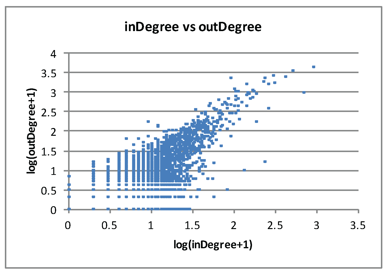The AS-level network has $27,106$ nodes (683 isolated) and $100,402$ directed edges; the graph length (diameter) is 6253, the density (number of edges divided by number of possible edges) is $1.9920\times {10}^{-5}$, and the average (in and out) degree is $3.70$, with ≈76.93% and $2.59$% of the nodes having zero indegree and outdegree, respectively. Figure 1 shows the indegree and outdegree distribution and Figure 2 shows the scatter plot of indegree and outdegree of the graph.

All the IDD games in the experiments presented in this section have this network structure.

For simplicity, we call Internet games the class of IDD games with the AS-level network graph and low ${\alpha }_i$ values. We considered various settings for model parameters of Internet games: a single instance with specific fixed values; and several instances generated at random (see

Table 1. Internet Games’ Model Parameters.

Model Parameters	Fixed: $\mathit{U}=0.5$ Random: $\mathit{U}\sim \mathbf{Uniform}\left(\right[0,1\left]\right)$
${\alpha }_i$	$\mathrm{U}/20$
$L_i$	${10}^8+\left({10}^9\right)\times \mathrm{U}$
$C_i$	${10}^5+\left({10}^6\right)\times \mathrm{U}$
${\widehat{p}}_i$	$0.9\times \frac{{\tilde{p}}_i}{{\tilde{p}}_i+{\sum }_{k\in \mathrm{Ch}\left(i\right)}{\tilde{q}}_{ik}}$
${\widehat{q}}_{ij}$	$0.9\times \frac{{\tilde{q}}_{ij}}{{\tilde{p}}_i+{\sum }_{k\in \mathrm{Ch}\left(i\right)}{\tilde{q}}_{ik}}$
$z_i$	$0.2+\mathrm{U}/5$
${\tilde{p}}_i$	$0.8+\mathrm{U}/10$
${\tilde{q}}_{ij}$	$z_i$$\frac{\left|\mathrm{Ch}\right(j\left)\right|+\left|\mathrm{Pa}\right(j\left)\right|}{{\sum }_{k\in \mathrm{Ch}\left(i\right)}\left|\mathrm{Ch}\left(k\right)\right|+\left|\mathrm{Pa}\left(k\right)\right|}$
$C_i^0$	${10}^6$

for details). The attacker’s cost-to-attack parameter for each node i is always held constant: $C_i^0={10}^6$. For each run of each experiment, we ran BRGD with randomly-generated initial conditions (i.e., random initializations of the players’ mixed strategies): $x_i\sim \mathrm{Uniform}\left([0,1]\right)$, i.i.d. for all i, and y is a probability distribution generated uniformly at random, and independent of $\mathbf{x}$, from the set of all probability mass functions over $n+1$ events. 14 The initialization of the transfer-probability parameters of a node essentially gives higher transfer probability to children with high (total) degree (because they are potentially “more popular”). The initialization also enforces ${\widehat{p}}_i+{\sum }_{j\in \mathrm{Ch}\left(i\right)}{\widehat{q}}_{ij}=0.9$. Other initializations are possible but we did not explore them here.

5.1. Computing an ϵ-MSNE Using BRGD

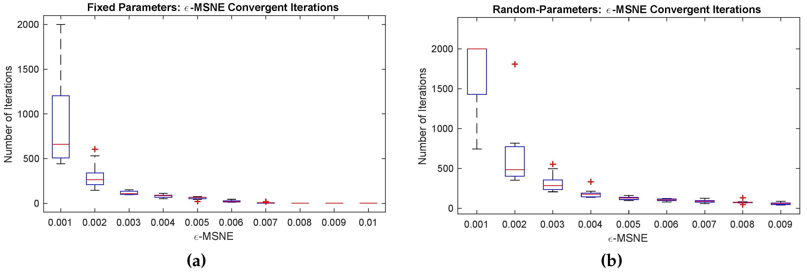
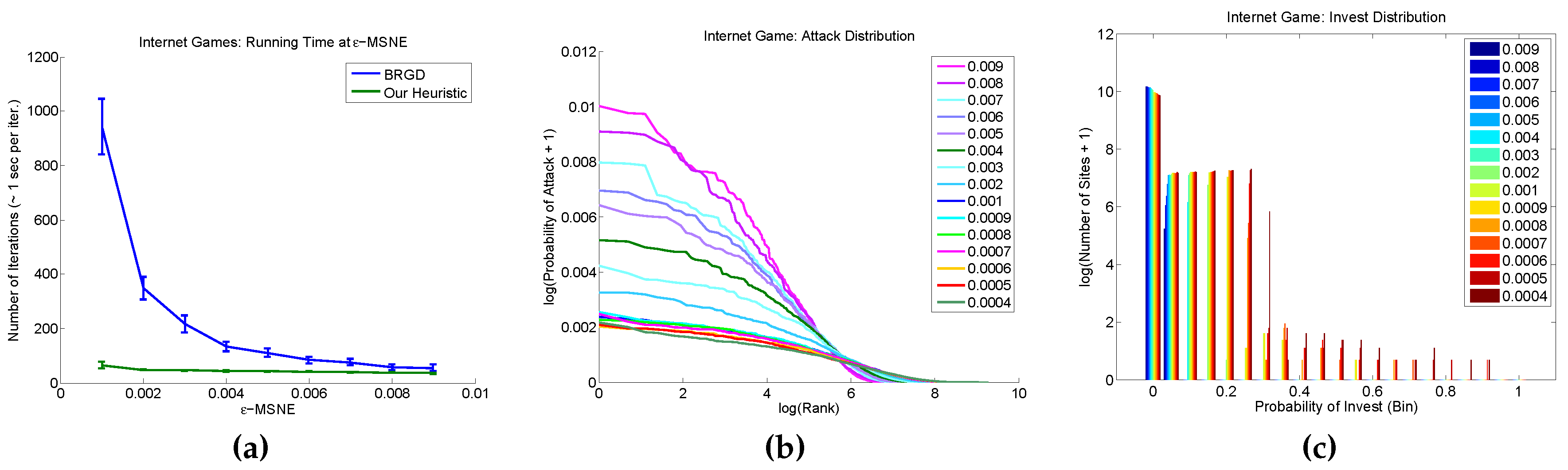
Given the lack of theoretical guarantees on the convergence rate of BRGD, we began our empirical study by evaluating the convergence and computation/running-time behavior of BRGD on Internet games. We ran ten simulations for each ϵ value and recorded the number of iterations until convergence (up to 2000 iterations). Figure 3 presents the number of iterations taken by BRGD to compute an ϵ-MSNE as a function of ϵ. All simulations in this experiment converged (except for $ϵ=0.001$, for which two of the runs on the single instance and all those on randomly-generated instances did not converge). Each iteration took roughly 1–2 s. (wall clock). Hence, we can use BRGD to consistently compute an ϵ-MSNE of a 27 K-players Internet game in a few seconds.

We now concentrate on the empirical study of the structural characteristics of the ϵ-MSNE found by BRGD. We experimented on both the single and randomly-generated Internet game instances. We discuss the typical behavior of the attacker and the sites in an ϵ-MSNE, and the typical relationship between ϵ-MSNE and network structure.

5.1.1. A Single Internet Game

We first studied the characteristics of the ϵ-MSNE of a single Internet game instance. The only source of randomness in these experiments comes from BRGD’s initial conditions (i.e., the initialization of the mixed strategies $\mathbf{x}$ and $\mathbf{y}$). BRGD consistently found exact MSNE (i.e., $ϵ=0$) in all runs.

Players’ Equilibrium Behavior

In fact, we consistently found that the attacker always displays only two types of “extreme” equilibrium behavior, corresponding to the two kinds of MSNE BRGD found for the single Internet game: place positive probability of a direct attack to either almost all nodes (Strategy A) or a small subset (Strategy B). Figure 4 shows a plot of the typical probability of direct attack for those two equilibrium strategies for the attacker when BRGD stops. In both strategies, a relatively small number of nodes (about 1K out of 27K) have a reasonably high (and near uniform) probability of direct attack. In Strategy A, however, every node has a positive probability of being the target of a direct attack, albeit relatively very low for most; this is in contrast to Strategy B where most nodes are fully immune from a direct attack. Interestingly, none of the nodes invests in either MSNE: $x_i^{*}=0$ for all nodes i. Thus, in this particular Internet game instance, all site nodes are willing to risk an attack.

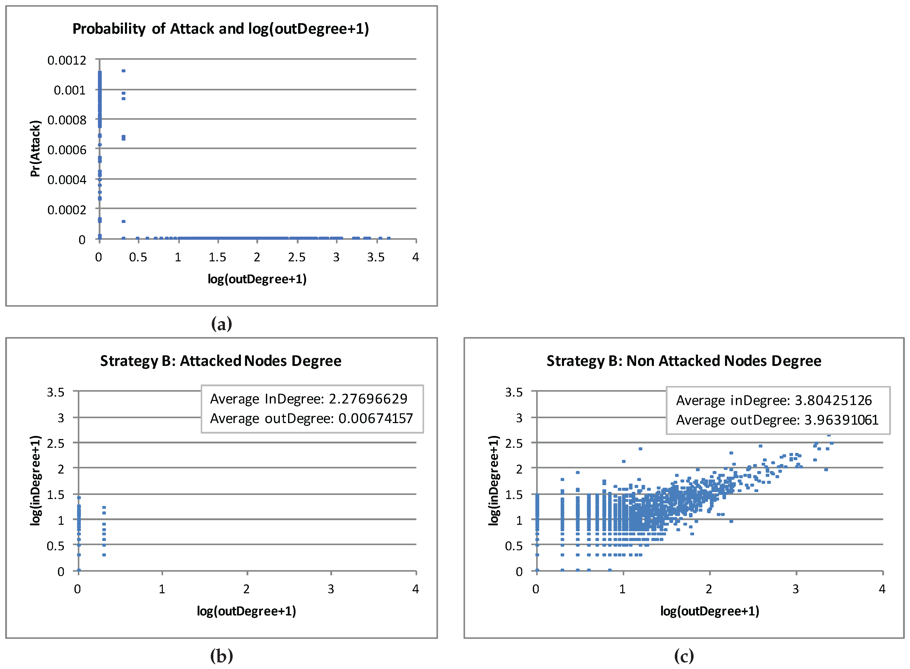
Relation to Network Structure

We found that the nodes with (relatively) high probability of direct attack are at the “fringe” of the graph (i.e., have low or no degree). In Strategy A, fringe nodes (with mostly 0 or 1 outdegree) have relatively higher probability of direct attack than nodes with higher outdegree. Similarly, in Strategy B, the small subset of nodes that are potential target of a direct attack have relatively low outdegree (mostly 0, and $0.0067$ on average; this is in contrast to the average outdegree of $3.9639$ for the nodes immune from direct attack). Figure 5 shows the relation between the probability of attack and outdegree and the relation between the indegree and outdegree of a typical simulation runs for strategy A and for Strategy B as described above, respectively. We emphasize that these observations are consistent throughout all runs of the experiment. In short, we consistently found that the nodes with low outdegree are more likely to get attacked directly in the single Internet game instance.

5.1.2. Randomly-Generated Internet Games

We now present results from experiments on randomly-generated instances of ten Internet games, a single instance for each $ϵ\in \{0.001,0.002,\dots ,0.009\}$. For simplicity, we present the result of a single BRGD run on each instance. 15

Behavior of the Players

Figure 6 shows plots of the attacker’s probability of direct attack and histograms of the nodes’s probability of investment in a typical run of BRDG on each randomly-generated Internet game instance for each ϵ value.

The plots suggest that approximate MSNE found by BRGD is quite sensitive to the ϵ value: as ϵ decreases, the attacker tends to “spread the risk” by selecting a larger set of nodes as potential targets for a direct attack, thus lowering the probability of a direct attack on any individual node; the nodes, on the other hand, tend to deviate from (almost) fully investing and (almost) not investing to a more uniform mixed strategy (i.e., investing or not investing with roughly equal probability).

A more thorough study confirms the above observation of the attacker and it is illustrated by Figure 7. Figure 7 shows: (a) the number of iterations taken by the smooth-best-response gradient-dynamics algorithm for ϵ-MSNE to converge (top left); (b) the number of nodes that are being targeted (top right); (c) the highest probability of attack (bottom left); and (d) the scatter plot of the nodes that are being targeted and the highest probability of attack (bottom right) for each of the ten simulations. From this figure, we observe that, as ϵ decreases, (1) the number of iterations takes for an ϵ-MSNE to converge increases (top left); (2) the number of nodes that are being targeted increases (top right); and (3) the highest probability of attack decreases (bottom left). From the bottom right graph of Figure 7, we observe that there is a negative correlation between the number of nodes that are being targeted and the highest probability of an attack: as the highest probability of an attack increases, the number of nodes that are being targeted decreases.

A possible reason to explain the behavior of the sites is that as more nodes become potential targets of a direct attack, more nodes with initial mixed strategies close to the “extreme” (i.e., very high or very low probabilities of investing) will move closer to a more uniform (and thus less “predictable”) investment distribution.

Relation to Network Structure

Figure 8 presents some experimental results on the relationship between network structure and the attacker’s equilibrium behavior. The graphs show, for each ϵ value, the average indegree and outdegree of those nodes that are potential targets of a direct attack at an ϵ-MSNE, across the BRGD runs of the ten randomly-generated IG instances. In general, both the average indegree and outdegree of the nodes that are potential targets of a direct attack tend to increase as ϵ decreases. One possible reason for this finding could be the fact that the values of ${\alpha }_i$ generated for each player are relatively low (i.e., uniformly distributed over $\left[0,\frac{1}{40}\right]$); yet, interestingly, such behavior and pattern, is the exact opposite of the theory for the case ${\alpha }_i=1$.

5.1.3. Case Study: A Randomly-Generated Instance of an IG at $0.005$-MSNE

In this subsection, we provide a detailed topological study of a randomly-generated IG instance at $0.005$-MSNE.

Topological Structure of an Attack to the Internet

In Figure 9, we plot the topological structure of the top sites (in this case 402) with the highest $y_i$ and their immediate neighbors at $0.005$-MSNE.

Notice that there are a few isolated nodes and a few small “node-parent-children” networks, but in general, the largest network component tends to have a cluster-like structure. Figure 9 also shows the number of connected components of the network for the subgraph of the nodes most likely to be attacked (and their neighbors), as well as those of the network for the subgraph of the nodes with the highest probability of investing, along with some additional properties of the graphs.

Figure 10 and Figure 11 show the indegree and outdegree of the (402) non-zero $y_i$ nodes and the remaining (26704) zero $y_i$ nodes, respectively. We did not observe in our experiments any strong relationship between the $y_i$’s or $x_i$’s in the ϵ-MSNE we found and the corresponding indegree or outdegree of the node i. However, we observed that, among the nodes with non-zero probability of attack, there was a slight tendency for those nodes with the lowest probability of attack to also have low outdegree and for those nodes with the highest probability of investing to also have low outdegree, but that tendency did not seem significant enough.

As mentioned earlier (Section 5.1.2), the behavior of the site players is quite sensitive to the ϵ value. Therefore, this could be one of the reasons that these nodes (with the highest $y_i$) have low outdegree.

5.2. A Heuristic to Compute ϵ-MSNE Based on Smooth Best-Response for the Attacker

In this subsection, we introduce an improved, simple heuristic to compute ϵ-MSNE on arbitrary graphs for lower ϵ values than those considered in the previous subsection (Section 5.1). Here, we evaluate the proposed hybrid BRGD-SBRD heuristic for computing ϵ-MSNE in IDD game using IGs randomly generated as described and used previously in this section.

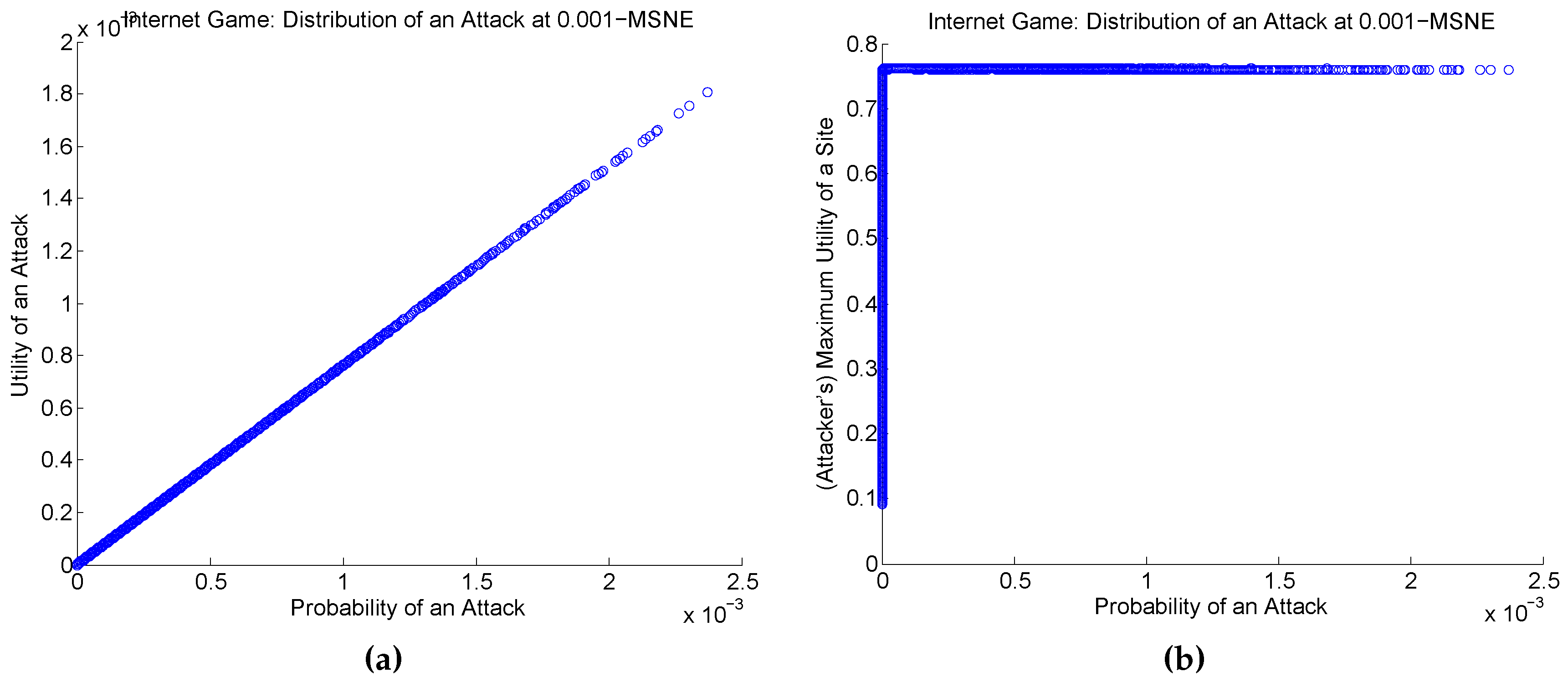
We first look at the attacker’s behavior at an ϵ-MSNE we obtain using BRGD in IGs. We generate a few IG instances and run BRGD until it converges to an ϵ-MSNE for $ϵ\in \{0.001,0.002,\dots ,0.009\}$. We observe that in a $0.001$-MSNE $({\mathbf{x}}^{*},{\mathbf{y}}^{*})$, (1) there is a positive, almost-deterministic correlation between the probability of an attack $y_i^{*}$ and each component $y_i^{*}{U}_i\left({\mathbf{x}}^{*}\right)$ of the expected utility the attacker obtained for each site i, where $U_i\left({\mathbf{x}}^{*}\right)$ is as defined in Equation 40, and (2) the attacker always target the sites with the highest potential utility ${max}_i{U}_i\left({\mathbf{x}}^{*}\right)$ (i.e., the maximum utility the attacker can get by attacking any site with probability 1). This observation is consistent with other IGs and holds across the different ϵ-MSNE for various ϵ values. Figure 12 shows evidence of this behavior. Indeed, the main take away is that the attacker tends to favor (or target) sites with highest expected utility. As observed, the attack seems to have some distributional form. Note that while one might expect this behavior given the way BRGD works, there is no theoretical guarantee for such behavior occuring at an approximate MSNE. This is because, in principle, any player may achieve a given approximation level without necessarily assigning a probability over each pure strategy in a way that is monotonically related to the expected payoff for executing that pure strategy deterministically, let alone the linear relationship we observe in the left-hand-side plot (a) of Figure 12. Similarly, given the last two statements, that the attacker is actually placing positive probability of attack only among those sites for which it would obtain highest maximum expected payoff, as the right-hand-side plot (b) of Figure 12 shows, is reassuring.

In what follows, we assume that the attacker is using smoothed best-response [35] and that the attack distribution is a quantal-response mixed strategy [53] (i.e., has the form of a Gibbs-Boltzmann distribution):

$$\begin{array}{c}\hfill y_i^{\lambda }\left(\mathbf{x}\right)\equiv \frac{exp\left(U_i(x_i,{\mathbf{x}}_{\mathrm{Ch}\left(i\right)})\right)/\lambda )}{{\sum }_{i=0}^{n}exp(U_i(x_i,{\mathbf{x}}_{\mathrm{Ch}\left(i\right)})/\lambda )},\end{array}$$

(45)

where $U_0(x_i,{\mathbf{x}}_{\mathrm{Ch}\left(i\right)})$ is the normalized version of $U(\mathbf{x},\mathbf{0})=0$ (i.e., after normalizing U to $[0,1]$), and λ is a positive constant. Thus, the attacker’s best-response correspondence is always a singleton, ${\mathcal{BR}}_0\left(\mathbf{x}\right)\equiv \left\{{\mathbf{y}}^{\lambda }\left(\mathbf{x}\right)\right\}$, and thus essentially a strictly positive, vector-valued function of $\mathbf{x}$, for any given λ. This update is the result a slight modification of the attacker payoff function that adds a “controlled” entropic term to favor “diverse” attack probabilities, where λ controls diversity (i.e., the level of non-determinism of the attacker’s best response): formally, given a positive real-value λ, the attacker’s payoff is now $U(x,y)+\lambda H\left(y\right)$, where $H\left(y\right)\equiv {\sum }_{i=0}^n{y}_{i}ln\frac{1}{y_i}$ is the standard (Shannon) entropy function. The interpretation of λ is that it controls the precision of the attacker and make the utility more distinct. The parameter λ is really the precision or temperature parameter of the Gibbs-Boltzmann distribution: increasing λ leads to the uniform distribution, while decreasing λ produces ϵ-MSNE with lower ϵ because λ restricts the effect of the entropic term in that case. In fact, at temperature $\lambda =0$, we recover the original best-response for the attacker.

The form for the attacker’s mixed strategy given in Equation (45) has several, natural attractive properties: (1) sites with high utility will have higher probability of an attack and (2) the respective expected utility and the probability of an attack are positively correlated (higher probability of attack implies higher expected utility gain). We observe these characteristics in our experiments (Figure 12).

Based on the previous discussion, we propose the following heuristic to compute ϵ-MSNE which refer to as the hybrid BRGD-SBRD heuristic. The heuristic starts by initializing all of the sites’ investment level $x_i$ to 0. It then updates the probability of attack for each site and increments the investment level of the site by a small amount (currently $0.001$) for sites that do not satisfy the following condition: $R_i\ge y_i{\widehat{p}}_i+(1-{\alpha }_i){\sum }_{j\in \mathrm{Pa}\left(i\right)}{y}_j(1-x_j){\widehat{q}}_{ji}$. The algorithm terminates either when all of the sites satisfy the condition or when it reaches the maximum number of iterations. The condition, $R_i\ge y_i{\widehat{p}}_i+(1-{\alpha }_i){\sum }_{j\in \mathrm{Pa}\left(i\right)}{y}_j(1-x_j){\widehat{q}}_{ji}$, for site i is the threshold for i to not invest. A nice property of this is that given the attacker’s Gibbs-Boltzmann distribution, for any site i, given the strategies of others, the attack decreases monotonically with $x_i$. As a result, no site has an incentive to unilaterally increase its investment to violate the constraint above. Consequently, to justify the use of the condition in the hybrid BRGD-SBRD heuristic in IGs, we observe that in all of the IGs we generated, the percentage of the sites at the $0.001$-MSNE we obtained that satisfies the above condition is ≥98%. The quality of an ϵ-MSNE obtained by the hybrid BRGD-SBRD heuristic depends on the percentage of the sites that satisfy the condition at an ϵ-MSNE. Note that if a high percentage of the sites does not satisfy the condition at the ϵ-MSNE, we can reverse the heuristic by initializing all of the sites investment level $x_i$ to 1 and lower the $x_i$’s until all sites satisfy the opposite constraint.

Algorithm 1 provides pseudocode for the resulting hybrid BRGD-SBRD heuristic, in which the attacker uses smooth best-responses while the sites use best-response gradient, to compute an approximate MSNE in arbitrary IDD games as discussed.

Algorithm 1: Heuristic Based on Hybrid of BRGD and Smooth Best-Response Dynamics (SBRD) to Compute an ϵ-MSNE in Single-Attack IDD Games

5.3. Evaluation of the Hybrid BRGD-SBRD Heuristic on Internet Games

To evaluate the hybrid BRGD-SBRD heuristic, we randomly generated ten IGs and compare the results to those obtained using BRGD exclusively.

The first question we address is, what is the relation between the constant λ and the actual approximation quality ϵ achieved in practice?

Table 2. Selection of the Constant λ for the Hybrid BRGD-SBRD Heuristic.

λ	Smallest ϵ
0.05	0.06
0.01	0.008
0.005	0.004
0.001	0.0009
0.0005	0.0006
0.0001	0.0004

shows the impact λ has on ϵ, for the smallest ϵ-MSNE we can obtain for an instance of the IGs (others are similar). The take-home message is that ϵ deceases with λ as expected. For the remaining of this section, we will fix $\lambda =0.001$ when comparing to BRGD as BRGD cannot find ϵ-MSNE beyond $0.0009$-MSNE within 10 K iterations (1 s per iteration).

5.3.1. Comparing Running Time of BRGD and the Proposed Hybrid BRGD-SBRD Heuristic

Next we study the convergence time to an ϵ-MSNE on the ten IG instances when using (1) BRGD exclusively and (2) the hybrid heuristic. We consider the running time in terms of the number of iterations that the algorithm takes to achieve a particular ϵ-MSNE. Each iteration is roughly 1 s for both BRGD and the hybrid heuristic. Figure 13a shows that the running time of the hybrid heuristic is considerably faster than BRGD. The rate at which the number of iterations increases as ϵ decreases seems extreme for the hybrid heuristic—it is almost constant—relative to that for BRGD. Not only is the hybrid heuristic faster than BRGD but it can also find ϵ-MSNE with lower ϵ values.

As an application, we could run our heuristic until it reaches an ϵ-MSNE or converges. Then use the output of our ϵ-MSNE to initialize BRGD. Figure 14 shows the relative improvement over the hybrid heuristic on some IGs. It improves our $0.001/0.0009$-MSNE to $0.0006$-MSNE.

5.3.2. Attacker and Sites’ Equilibrium Behavior

We study whether the equilibrium behavior of the attacker and sites that we observed and discussed in Section 5.1 remains the same, or is similar, as we lower ϵ. The following results are a direct output of our heuristic. Figure 13b shows the attack distribution (left) and the investment distribution (right) at ϵ-MSNE, for different ϵ values, on an IG instance. Our results are consistent with those in Section 5.1, and persist for lower ϵ values. We see that as ϵ decreases, the attacker targets more sites while lowering the probability of the direct attack, and more sites move from not invest to partially invest.

5.3.3. Network Structure of an Attack

Next, we present experimental results on the average indegree and outdegree of the targeted sites at ϵ-MSNE to understand the “network structure of the attack” as we did in Section 5.1. Figure 15 shows exactly this. To summarize our experimental results, we can clearly observe that as ϵ decreases both the average indegree and outdegree increase. The results for lower ϵ values indicate the average indegree and outdegree are stabilizing and converging as ϵ decreases. This is also consistent with the observations made in Section 5.1. This consistency also adds evidence to the effectiveness of our proposed heuristic for very low ϵ values.

6. Future Work, Open Problems, and a Summary of Our Contributions

We end by discussing future work and some open problems, and providing a brief summary of our contributions.

6.1. Future Work

In this subsection, we discuss potential avenues of future work.

6.1.1. Attackers Can Affect Transfer Probabilities

We could extend the strategy space of the attacker by allowing the attacker to affect transfer. One particular instantiation of this idea is to have the network graph edges represent the attacker’s targets, as opposed to just the node. The attacker’s pure strategies would now be based on the edges $(i,j)$, such that binary action variable $b_{ij}$ would now represent the attack, taking a value of one if the attacker wants to attack j but only via a transfer from i.

6.1.2. Multiple Attackers with Multiple Attacks

While dealing with multiple attackers is outside the scope of this paper, we have in fact extended the model in a natural way in that direction. We refer the reader to Appendix E for a discussion of this setting. In short, we were able to extend the representation results, but not the characterization or computational/algorithmic results. We leave that endeavor for future work. In principle, we can use BRGD and the hybrid BRGD-SBRD as heuristics in the case of multiple attackers.

6.1.3. Learning IDD Games

Another interesting research direction is the adaptation of machine-learning techniques to infer IDD games from data for the purpose of compactly representing stable outcomes and performing strategic inference.

6.1.4. Other Open Problems

A thorough characterization of the equilibria of interdependent defense games is lacking, specially for the case of multiple potential attacks by multiple aggressors. Also, we need a better understanding of the effect of network structure of the game and restrictions on the aggressors’ available strategies on the equilibria of the game.

Many computational problems in the context of interdependent defense games remain open.

• What is the computational complexity of the problem of computing equilibria of single-attack IDD games with arbitrary transfer vulnerability? (e.g., a single, multiple or all MSNE? MSNE with particular properties?)
• What is the computational complexity of the problem of identifying “influential” agents, in the sense of Irfan and Ortiz [41] (see also, Kleinberg [54] and the references therein)?
• How is the complexity affected by network structure or restrictions on the aggressors’ available strategies? While we provide FPTAS for approximate MSNE in single-attack IDD games with arbitrary transfer vulnerability values and directed tree graphs over the sites, it is fair to say that there is more work to do in that direction. A particularly interesting question is whether we can establish PPAD-completeness results for arbitrary single-attack IDD games. That would strengthen the hardness (NP-complete) result we present in Section 4.2. The relationship between single-attack IDD games and graphical polymatrix games seems particularly close. Perhaps one may be able to apply existing results on the PPAD-completeness of certain classes of graphical polymatrix games to establish PPAD-completeness in our context. A promising direction is to pursue potential reductions using results such as those of (Cai and Daskalakis [50], Theorem 1.2) and (Daskalakis et al. [29], Lemma 6.3) on (graphical) polymatrix games with “strictly competitive games on the edges” and on 3-additive graphical Nash, respectively.

6.2. Summary of Contributions

In this paper, we propose IDD games, an adaptation of IDS games to the setting in which the attack is deliberate and the attacker is explicitly modeled. We consider the special case of the single attack scenario as a way to limit the attackers power, and prove that no PSNE exists in such subclass of games. We then consider randomized strategies and derive the appropriate expressions for the expected costs of the internal players and the expected payoff of the attacker, and consequently their respective best-response correspondences.

We study in depth the case in which only one attack is possible and investment in security does nothing to protect the players from the transfer risk (which is the same implicit assumption made in the original IDS work). We completely characterize the MSNE of such a subclass of IDD games. We prove that almost every game in that subclass has a unique MSNE, which can be almost-fully determined analytically.

That result immediately lead to a simple algorithm for computing the equilibrium that only requires a sorting of the cost-to-expected-loss ratio gain of the attacker for each player. Hence, the algorithm runs in $O(nlogn)$, where n is the number of internal players.

We then discuss some corollaries of the characterization and highlight the connection between the network structure and the investment of players at equilibrium. In particular, we show how investment probabilities at equilibrium essentially reflect some degree of “cooperation” (in a fully non-cooperative setting). It turns out that, at an equilibrium, players want to protect their own children in the network graph. That is, each player i wants to protect the set of players to which player i can transfer). Yet, somewhat counterintuitively at first, each player i’s security investment level has no direct dependence on the player’s parents, who are the true source of the risk to the player. In particular, we show how the probability of investment can is directly proportional to the fixed, but arbitrary number of children in the given directed network.

We also provided a hardness result for computing exact MSNE in arbitrary single-attack IDD games. We also designed an FPTAS to compute an ϵ-MSNE in graph with directed trees over the sites, despite the fact that the attacker’s payoff is a function of all the sites.

Finally, inspired by problems in cyber and network security, we designed a generator of random instances of IDD games based on a real-world instance of the AS-level Internet graph. We call the resulting instances Internet games (IGs) . We studied simple heuristics based on BRGD, SBRD, and a hybrid, for computing approximate MSNE in IGs. We evaluated the running times of the different heuristics and found that BRGD, when run exclusively, seems to be effective at computing ϵ-MSNE for ϵ values as low as $0.001$. We studied the characteristics of the approximate MSNE that BRGD produces in terms of both sites’ and attacker’s behavior and the relationship to the IGs network structure. We then proposed and studied a hybrid BRGD-SBRD heuristic in which the attacker uses SBRD while the sites use BRGD. It allows us to compute ϵ-MSNE with an order of magnitude lower in ϵ values very quickly in IG instances. Using the hybrid heuristic we successfully verified some of the conclusions we had obtained using BRGD alone, but now consider considerably lower ϵ values. We also showed how we can improve the effectiveness both in terms of speed and quality when using BRGD alone, by first running the hybrid heuristic and then starting BRGD alone from the ϵ-MSNE values that the hybrid heuristic found.

We view our work as an initial illustration of the potential for the type of quantitative analysis that may be possible in network security settings, even at the real-world Internet scale.
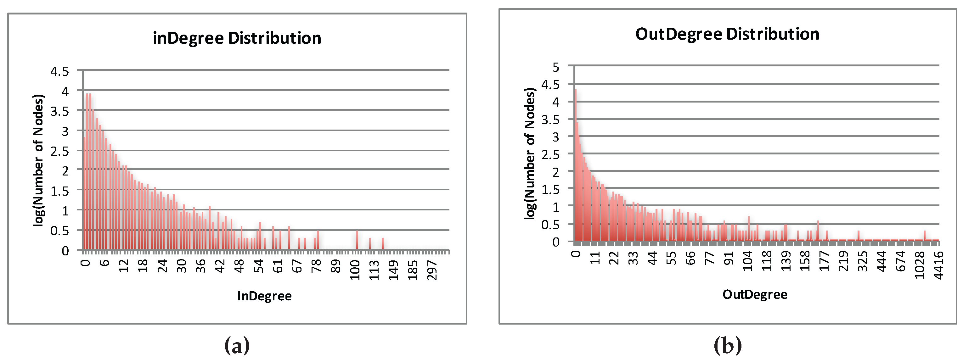
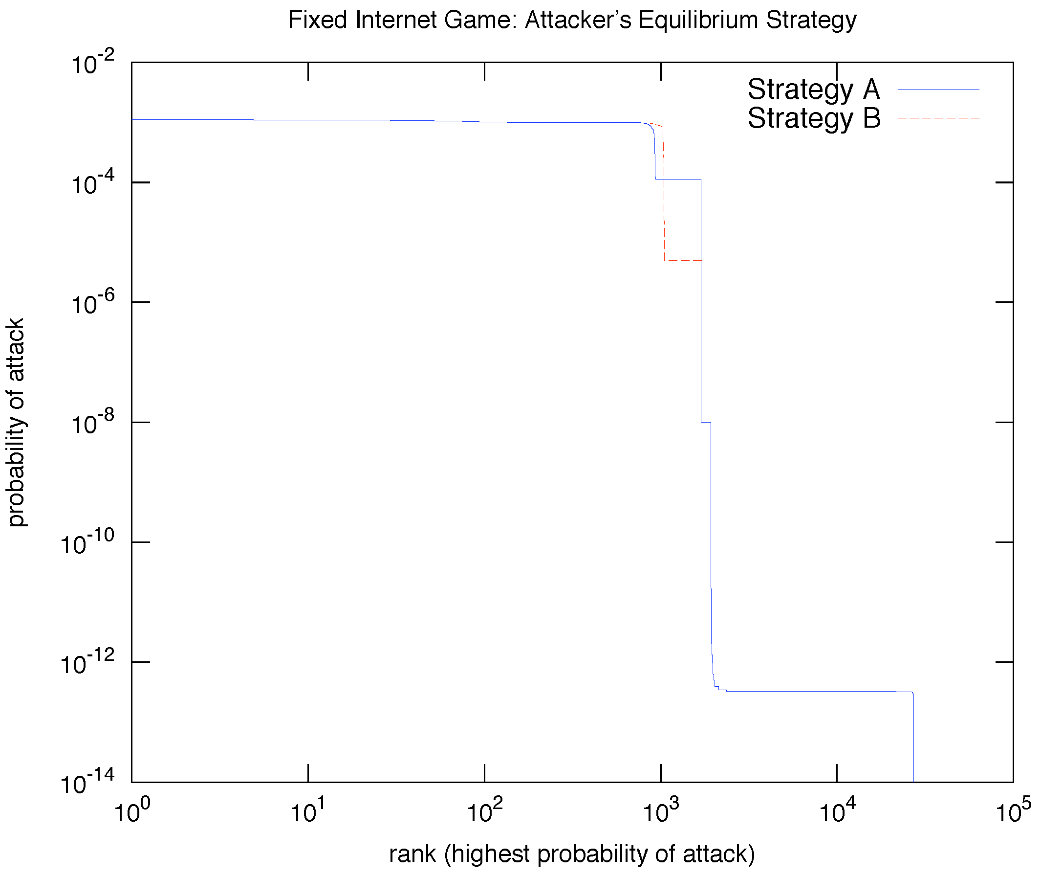
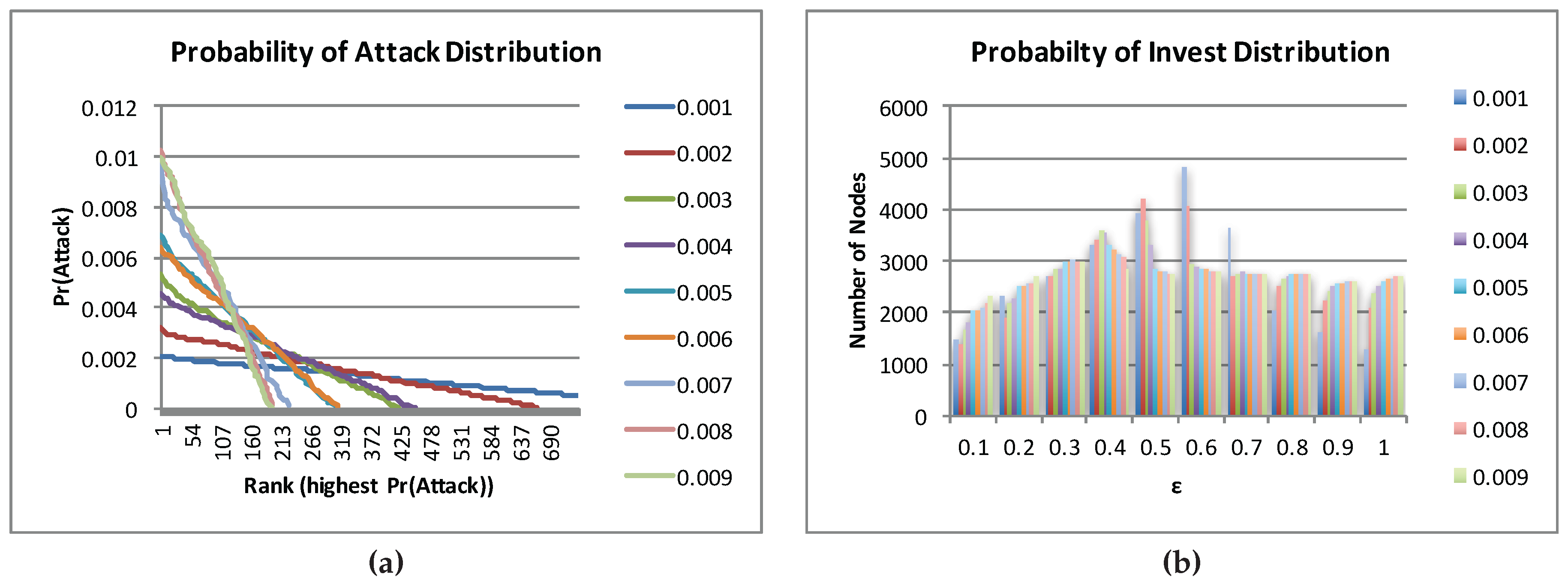
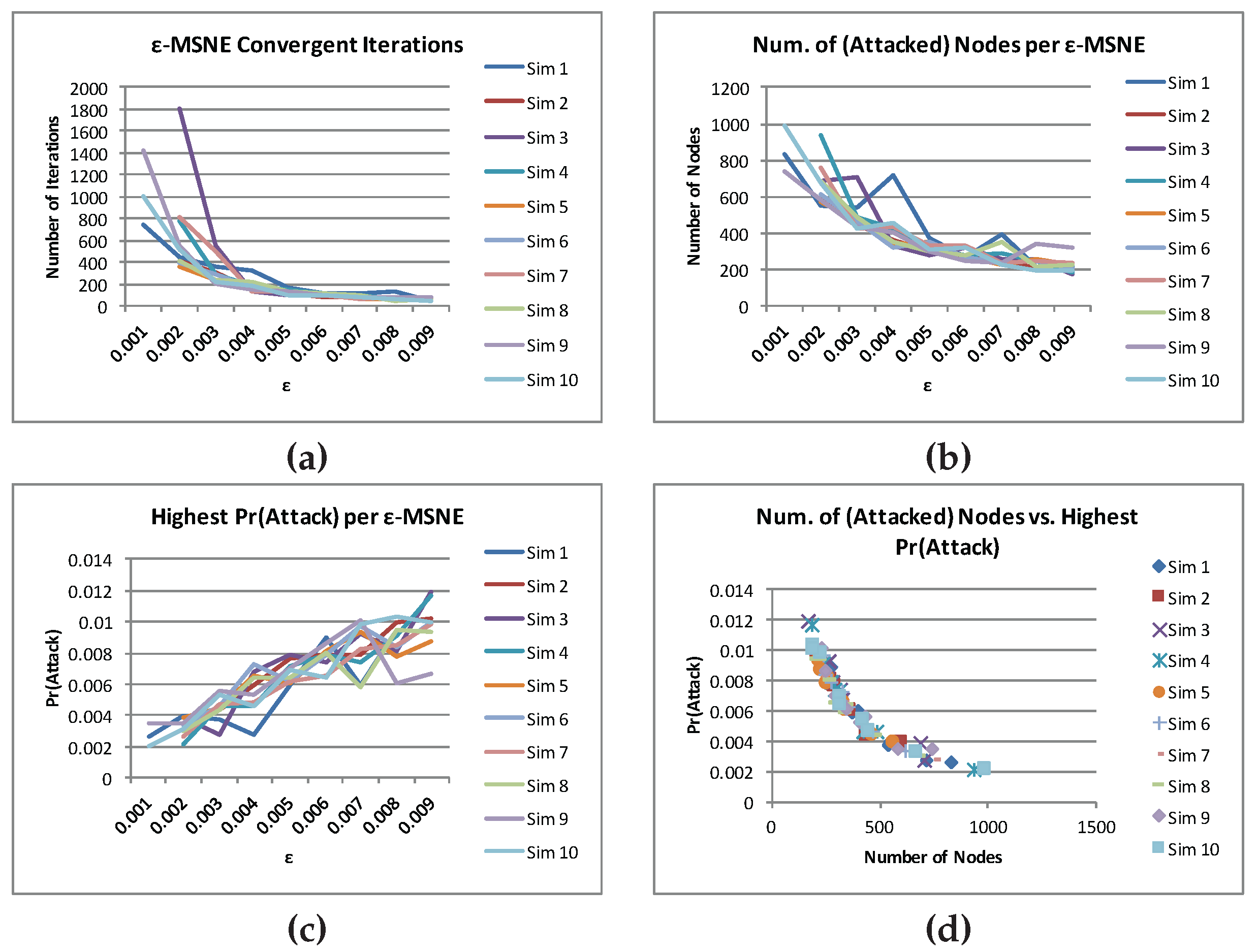
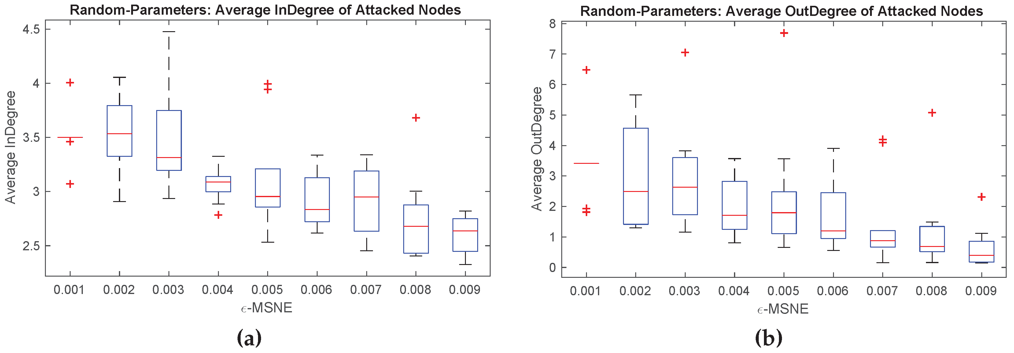
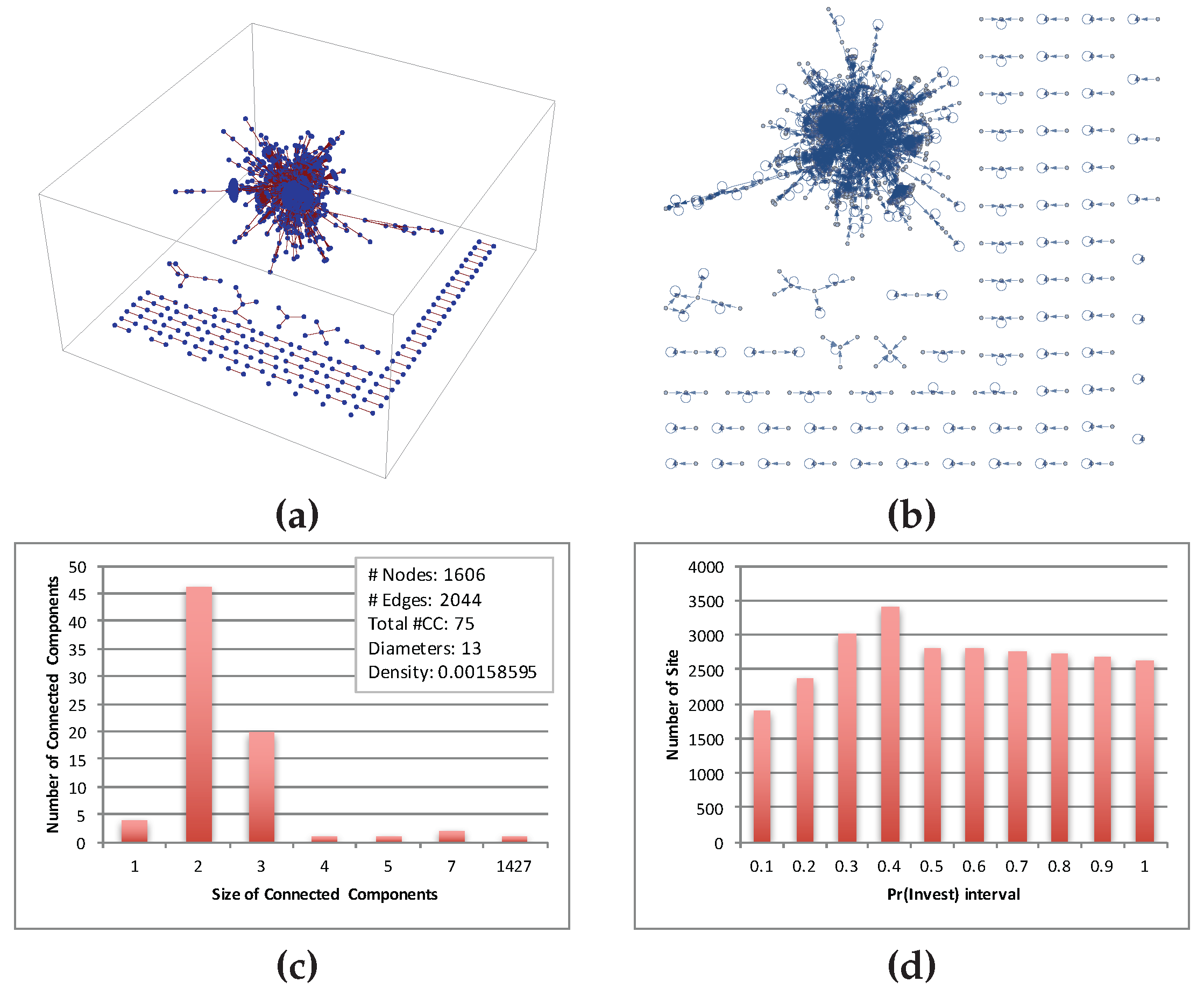
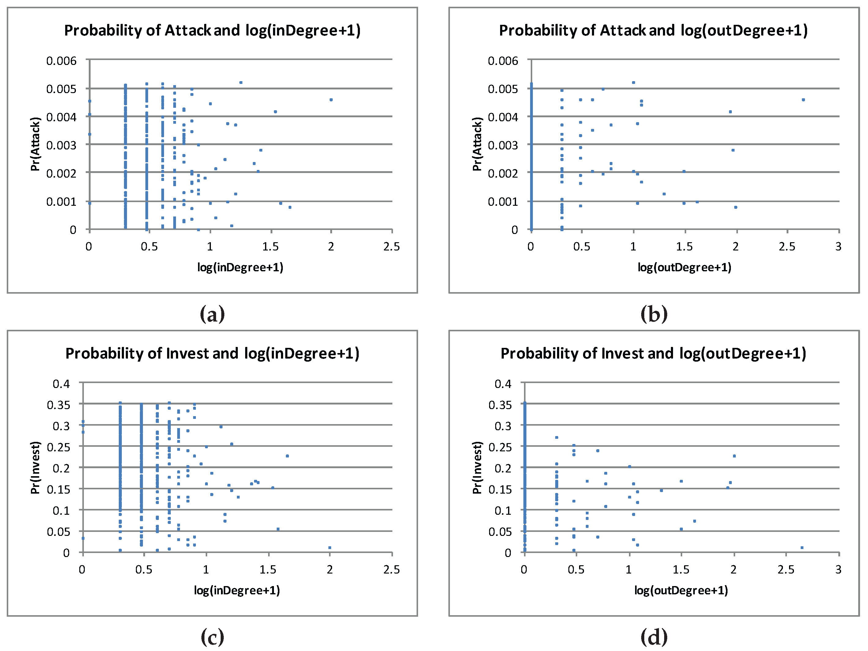
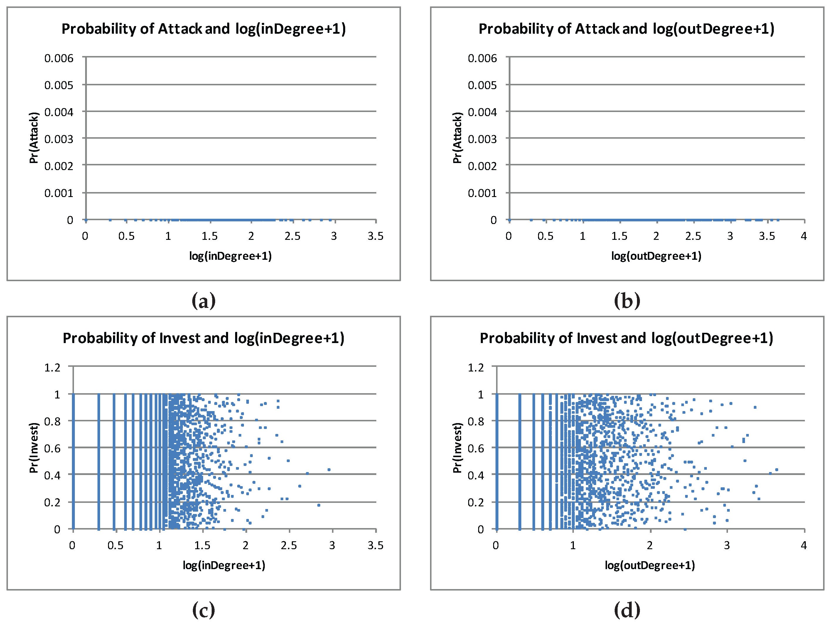
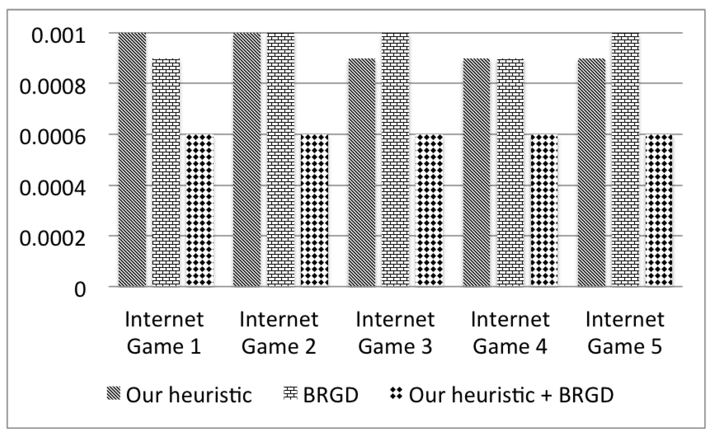
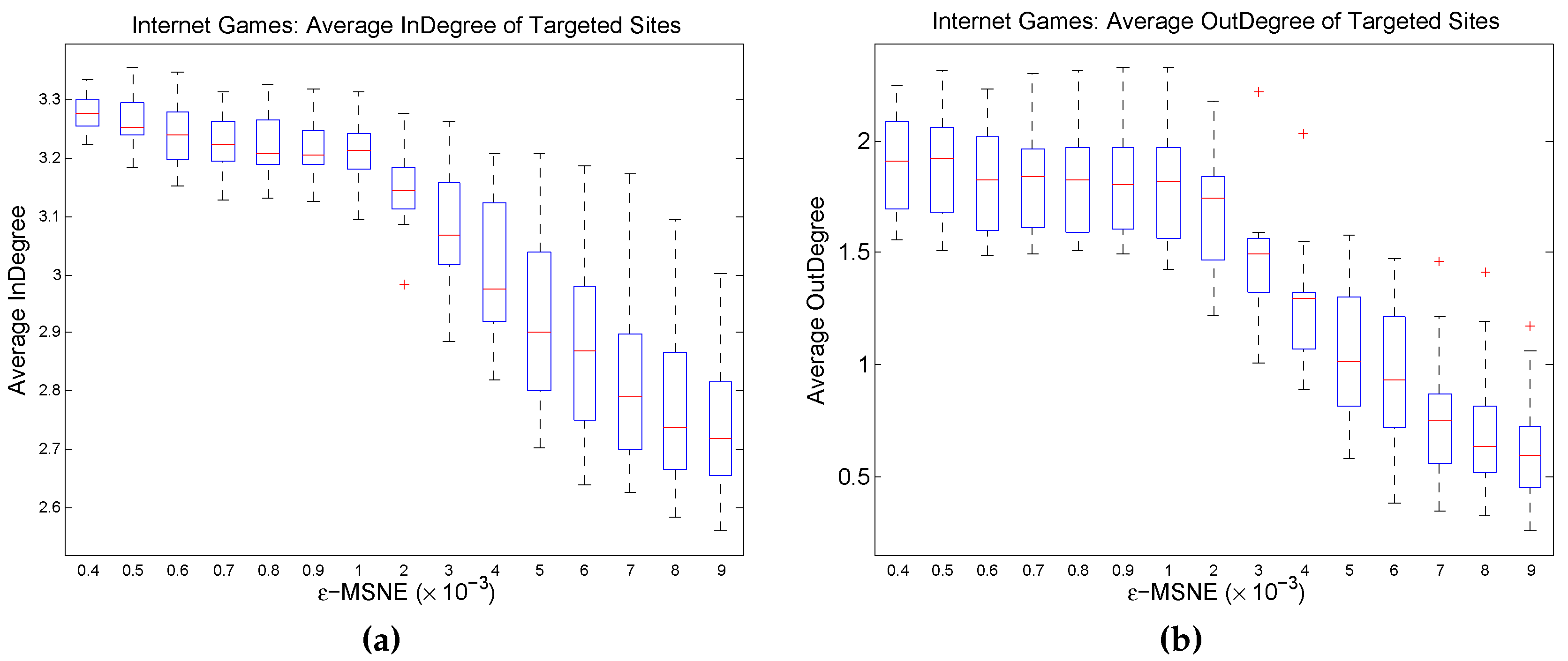