Creating a Domain of Losses in the Laboratory: Effects of Endowment Size

Department of Economics, Southern Illinois University, Carbondale, IL 62901, USA
Games 2018, 9(1), 13; https://doi.org/10.3390/g9010013
Submission received: 7 December 2017
/
Revised: 11 February 2018
/
Accepted: 18 February 2018
/
Published: 2 March 2018
Abstract
:This study examines the effects of initial endowment size on individual behavior in a binary choice game with no dominant strategy. Subjects make decisions in two, theoretically identical sequences, differing in initial endowment levels only. Each decision involves a choice between an option with a certain loss and an option with a loss that is increasing in the number of individuals who choose it. For the higher endowment level, all subjects are guaranteed a positive payoff. For the lower endowment level, subjects who choose the uncertain loss option could receive a negative payoff. The results indicate that in the first round of play, subjects with the higher endowment level choose the certain loss option significantly more often than subjects with the lower endowment level. There are, however, no significant differences in behavior beyond the first few rounds of play.
1. Introduction
Multiple laboratory experiments have shown that the frame of a decision environment matters. In particular, positive or gain framed and negative or loss framed decision environments have been shown to result in differing behavior. Andreoni (1999) [1] found that in a linear public goods game, subjects were much more cooperative under a positive frame than a negative frame. Park (2000) [2] and Sonnemans et al. (1998) [3] found similar results, which were later decomposed into different components in Cox (2015) [4]. Thus, we must use the appropriate frame for a given application in the laboratory, and for many applications, the relevant frame we need to use is the negative or loss frame. Implementing an experiment in this “domain of losses”, however, proves challenging, since we would have a difficult time conducting an experiment in which subjects pay us at the end of the experiment. The traditional and most common method of implementing a domain of losses in the laboratory is to give subjects sufficiently high initial endowments from which they may incur a loss, so as to guarantee a positive payoff in the end. The question then becomes, does the size of this initial endowment affect behavior when using this methodology? If it does, then we must take this into consideration when designing future experiments and interpreting their results.
Several studies have shown that individual behavior in laboratory experiments may be significantly affected by the size and origin of initial endowments. Though not specifically in the loss domain, Thaler and Johnson (1990) [5] find a “house money effect”, or increased risk-seeking behavior following a windfall gain. Comparable results were found by Rosenboim and Shavit (2012) [6] and Davis et al. (2010) [7]. This “house money effect” has also been translated to increased generosity in dictator games [8,9], and charitable giving [10]. Specific to the domain of losses, Etchart-Vincent and L’Hariden (2011) [11] investigate risk aversion in a domain of losses, compared across three different payment conditions: “real losses”, “losses-from-an-initial-endowment”, and “hypothetical losses”. Contrary to some of the above-mentioned studies, Etchart-Vincent and L’Hariden do not find any significant differences in behavior for the three payment conditions in the loss domain, although they do find some differences in a gain domain.
The goal of this study is to investigate whether initial endowment size significantly affects behavior in a decision environment framed in a domain of losses in which no player has a dominant strategy. Based on the games in Sorensen (2015) [12], subjects begin with an initial endowment and face a decision between an option with a certain loss and an option with a loss that is increasing in the number of individuals who choose it. The exact parameterizations are chosen so that no player ever has a dominant strategy, and initial endowment levels are varied so that in one of the two decision sequences subjects may incur a loss greater than their endowment (i.e., receive a negative payoff). To avoid the obvious problem of subjects owing the experimenter money at the end of a session, each subject participated in two sequences of decision rounds, one with a higher endowment level used in [12], and one with a much lower endowment level. This design ensures that each subject’s total earnings across both sequences are positive, while still allowing earnings to potentially be negative in one of the two sequences.
The results indicate that, in the early rounds, individuals choose the certain loss option more often in sequences with a higher endowment level, but this difference does not persist beyond the first few rounds. Thus, when using the traditional method of handling a domain of losses by giving subjects a sufficiently high initial endowment to guarantee positive payoffs, caution should be used in evaluating early round results. However, the results in this paper indicate that endowment size does not otherwise appear to matter.
2. Results
Section 2.1 below contains the theoretical model and theoretical predictions. Section 2.2 contains the experimental results.
2.1. Theoretical Model and Predictions
The basic game is identical to the asymmetric, non-probabilistic game in [12]. A group of N agents, each with an initial endowment, , must each choose one of two options. Option A or Option B 1. There are two types of agents, High-loss and Low-loss. There are High-loss agents and Low-loss agents, where . If an agent of either type chooses Option A, then they pay some cost, , where , and they keep with certainty. If an agent of either type chooses Option B, then they incur some loss, where the size of this loss is type-dependent and is increasing in the number of agents who choose Option B. If a High-loss agent chooses Option B, then their loss is , where is the number of agents who choose Option B, and is strictly increasing in . If a Low-loss agent chooses Option B, then their loss is , with strictly increasing in , and for all . Thus, if a High-loss agent chooses Option B, they keep , and if a Low-loss agent chooses Option B, they keep .
The experiments in this paper correspond to the following parameterization of the game 2:
, , , , , . For half of the decision sequences , and for the other half . Table 1 and Table 2 below outline the corresponding payoffs for both types of agents and each endowment level.
Note that for the higher of the two endowment levels, , while the payoff from Option B may be higher or lower than the payoff from Option A, depending on what others choose, the payoff from Option B is always positive. On the other hand, when the endowment is lowered to , the payoff from Option B may be negative if enough agents choose Option B.
As shown in [12] for , there is a unique pure-strategy Nash equilibrium in which both High-loss agents choose Option A and all four Low-loss agents choose Option B. However, the social optimum is for four agents to choose Option A (the two High-loss agents plus two of the Low-loss agents). It is easy to show that decreasing the endowment to does not change the Nash equilibrium or the social optimum.
2.2. Experimental Results
Table 3 below contains the proportion of individuals who chose Option A by endowment level, sequence order, and round. “S1” denotes sequence 1, and “S2” denotes sequence 2 3.
Comparing columns 2 and 3 of Table 3, as well as comparing columns 4 and 5, subjects appear to initially choose Option A more often when e = 25 than they do when e = 7. In sequence 1, 40% of subjects chose Option A in round 1 when e = 25, but only 13% of subjects chose Option A in round 1 when e = 7. This difference, however, does not persist past the first round. In sequence 2, the numerical values are different, but the relationship between endowment levels is unchanged. In sequence 2, 60% of subjects chose Option A in round 1 (round 11 overall) when e = 25, but only 33% of subjects chose Option A when e = 7. Again, this difference in behavior diminishes after the first round. When looking at the averages across all rounds, the percentage of individuals choosing Option A under the higher endowment level is slightly higher than under the lower endowment level (41% vs. 37% in sequence 1; 44% vs. 38% in sequence 2), but this appears to be driven by the early rounds of play, since there is no difference in these averages across rounds 6–10 for sequence 1, and there is only a slight difference for sequence 2 (44% vs. 42%).
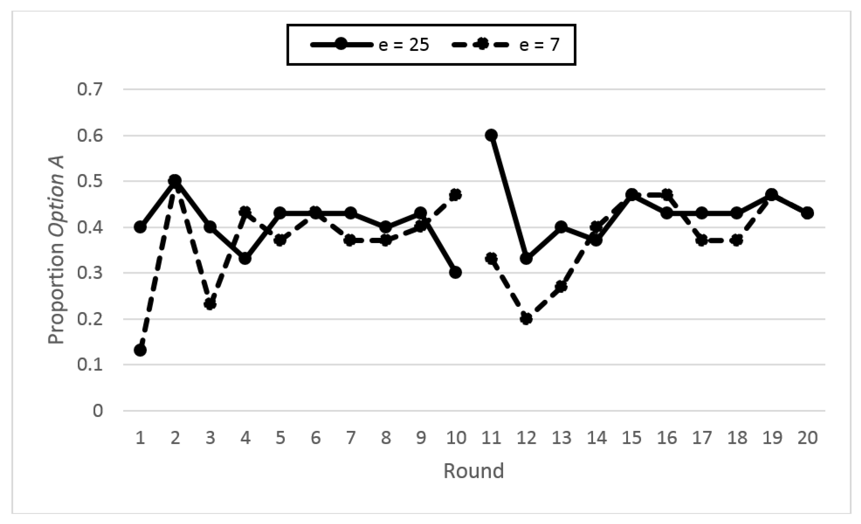
This information is also depicted in Figure 1 below. All rounds of both sequences are indicated on the horizontal axis, with rounds 1–10 corresponding to the first sequence within a session, and rounds 11–20, the second sequence.
Comparing the two endowment levels across rounds, there only appears to be a notable difference in round 1 of sequence 1 (Round 1 in Figure 1), and in the first three rounds of sequence 2 (Rounds 11–13 in Figure 1). For these rounds, the higher endowment level results in a greater proportion of individuals choosing Option A than the lower endowment level. As discussed above, this difference does not appear to persist 4.
Now turning to a statistical analysis of the data, the second row of Table 4 contains the results of a logistic regression with random effects, treating the data set as a panel with subjects as the cross-sectional dimension and round as the time dimension. The dependent variable, option choice, is equal to 1 for a choice of Option A and equal to 0 for a choice of Option B. The independent variable of interest, endowment, is reported in the second column, and is a dummy variable equal to 0 for e = 7 and 1 for e = 25. Also included in the regression are dummy variables for sequence (equal to 0 for sequence 1 and equal to 1 for sequence 2) and subject type (equal to 0 for Low-loss and equal to 1 for High-loss), as well as a constant.
The coefficient on endowment is positive and significant at the 90% confidence level, indicating that, overall, individuals chose Option A more often when e = 25, than when e = 7. Thus, endowment size may in fact matter. The coefficient on subject type is also positive and significant (at the 99% confidence level), indicating that High-loss subjects chose Option A more often than Low-loss subjects. This is what we would expect to see, based on the payoffs presented in Table 1 and Table 2, since High-loss subjects received lower payoffs from choosing Option B than Low-loss subjects did.
This positive and significant effect of endowment may be misleading, however. As we noted earlier, differences in behavior across endowment levels appear to decrease substantially after the first round. To test this observation, rows 3–12 of Table 4 contain the results of ten additional logistic regressions, separated by round. These additional regressions include the same dependent variable (option choice) and independent variables (endowment, sequence, and type) as the initial regression. Also, the data for the same rounds in both sequences were pooled. That is, the “Round 1” logistic regression includes data from rounds 1 and 11, “Round 2” contains data from rounds 2 and 12, and so on.
Looking at the second column, our initial observations are confirmed. Endowment has a positive and significant effect (at the 99% confidence level) in round 1, indicating that subjects with the higher endowment level do initially choose Option A more often. This difference in behavior quickly disappears however, with no significant effects after the third round. Thus, the significant effect we saw in the initial regression was being driven by the very large differences in behavior in early rounds of play. On the other hand, the positive and significant coefficient on “Type” only gets greater in magnitude and significance level as the rounds progress. Again, this is what we would expect based on their possible payoffs.
3. Discussion
3.1. General Discussion
Overall, the results indicate that when using initial endowments to create a domain of losses in the laboratory, the size of the endowment may have a significant impact on behavior in early rounds. In this study, there is a significant difference in behavior across endowment levels in the first decision round of each sequence, with individuals choosing the certain loss option more often when given the higher initial endowment. This difference decreases substantially after the first round however, and there are no significant differences in behavior across endowment levels after the third round in each sequence. Thus, if we look past the early rounds of play and focus our analysis on later rounds, endowment size does not appear to matter.
The main implication of these results is that in games like the one considered in this study, we can successfully utilize initial endowments to create a domain of losses (and guarantee positive payoffs) if we disregard behavior in early rounds of play. This allows for a relatively easy design and implementation of laboratory experiments in the loss domain. We should, however, use caution when interpreting early round results, since these may be significantly affected by the chosen endowment level.
3.2. Relationship to Loss Aversion and Market Entry Games
Both treatments (e = 25 and e = 7) include the exact same loss sizes from each option choice and all possible outcomes. A subject who chooses Option A loses 7 ECU, regardless of their initial endowment size. Similarly, while the loss from a choice of Option B does depend on the choices of others, it is the same across endowment levels for each possible outcome. This is how the experiments in this study were framed, in the domain of losses. If this is also how the subjects perceived the two treatments, then based on traditional loss aversion and prospect theory (see Kahneman and Tversky, 1979 [13]), there should be no differences in behavior across the two endowment levels. If, however, subjects instead considered only the final possible payoffs (initial endowment minus losses) and viewed these to be the gains or losses they were choosing from, then the two treatments are not identical from a loss aversion perspective.
With the lower endowment level (e = 7), Option B payoffs could be positive or negative. Even though all of these are the result of an initial loss, they may have been viewed as gains when they were positive and losses only when they were negative. Similarly, all payoffs for the high endowment level (e = 25) may have been viewed as gains, since the endowment was greater than the greatest possible loss. If this is the case, then traditional loss aversion would predict that we would see fewer choices of Option B for the low endowment level than for the high endowment level. However, the early-round results discussed in Section 2 and Section 3.1 above show the exact opposite. Subjects initially chose Option B significantly more often in the low endowment treatment.
This seemingly contradictory initial result may be explained by the type of risk present in this particular game. Loss aversion and prospect theory as originally described involve risk in the traditional sense, where potential gains or losses are dependent on chance to at least some degree. The game in this paper does not contain any risk in this sense but does contain strategic risk through the dependence of Option B payoffs on others’ choices. While strategic risk is still a type of risk, it makes one’s choices arguably more dependent on their beliefs over others’ actions. If individuals initially believed that fewer members of their group would choose Option B when e = 7 than they would when e = 25, then this could explain why we initially see more Option B choices for the lower endowment level. Subjects should quickly learn that such beliefs are incorrect, which would also explain why we see no significant differences in behavior across endowment levels in later rounds. Unfortunately, we do not have a report of subjects’ beliefs during the experiments, and so we cannot verify this hypothesis.
Comparable results have been found in market entry games (see Erev et al., 2010 [14]). The game in this paper is very similar to that of a market entry game, where the choice to “stay out” yields a certain payoff and the choice to “enter” yields a payoff that is decreasing in the number of individuals who choose it. In this sense, the “stay out” option is similar to the Option A choice in this paper, and the “enter” option is similar to the Option B choice. The main difference between the two games is the frame. The market entry game is typically framed either in the gain domain only, or in both the gain and loss domain. The game in this paper was framed entirely in the loss domain, with all outcomes and option choices leading to a loss of varying degrees. As discussed above however, this is not necessarily how the decision environments were viewed by the subjects, making the comparison between the game in this study and the market entry game even more relevant. Indeed, Erev et al. [14] report “excess entry” in a parameterization of the market entry game similar to the low endowment game in this paper. The games differ somewhat substantially however, since there is both strategic and traditional risk in the games in [14], with even the “stay out” option having a probabilistic payoff. Additionally, the subjects in [14] were not given a copy of the payoff structure, instead learning the game through feedback between rounds. In this study, subjects knew the complete payoff structure for both treatments before starting the first round.
4. Materials and Methods
Subjects are randomly placed into groups of six. Within each group, two subjects are randomly selected to be High-loss subjects and the other four are Low-loss subjects 5. Each subject participates in two sequences of ten decision rounds each. For one of the two sequences, each subject begins each round with an endowment of 25 Experimental Currency Units (ECU), and for the other sequence they begin each round with an endowment of 7 ECU. Subjects maintain their same group and type assignment within each sequence, but are randomly regrouped and types are randomly reassigned between sequences. In each round of each sequence, subjects must select Option A or Option B. Any individual who chooses Option A must give up 7 ECU. If an individual of either type chooses Option B, then the number of ECU they must give up depends on the actions of their group members. For each possible outcome, High-loss subjects who choose Option B must give up more than Low-loss subjects who choose Option B. The resulting payoffs are equal to the payoffs in the model discussed in Section 2.1, and outlined in Table 1 and Table 2 above.
The experiments consisted of four sessions conducted in the fall of 2013 with a total of 60 Indiana University students. Subjects were undergraduates from a variety of majors, recruited using the Online Recruitment System for Economic Experiments (ORSEE) (Greiner 2004 [15]). In two of the four sessions, subjects participated in the sequence with first, and in the other two sessions subjects participated in the sequence with first. Subjects were informed that they would be participating in two distinct sequences of decision rounds, but they were not given any information about how or if these two sequences differed. The experiment was computerized using z-Tree (Fischbacher 2007 [16]), and each session lasted approximately one hour. All subjects gave their informed consent for inclusion before they participated in the study. The study was conducted in accordance with the Declaration of Helsinki, and the protocol was approved by the IRB of Indiana University (Protocol #1303010585).
At the start of each session, subjects read through general instructions on computer monitors. The experimenter also presented these instructions on a screen at the front of the room. Subjects then proceeded to read the instructions for the first sequence of decision rounds. Again, the experimenter presented these instructions at the front of the room. Subjects were also given hard copies of all payoff tables contained in the instructions for the first sequence. In the instructions, subjects were told that both option choices involved a loss. The loss from choosing Option A was fixed at 7 ECU, and the loss from choosing Option B depended on their group members’ choices. The exact possible losses from choosing Option B were presented to the subjects through the payoff tables only. It was also through these tables that subjects were able to see that Option B payoffs could potentially be negative in the low-endowment sequence. When the experimenter presented the instructions and tables to the subjects, they made sure to mention that these Option B payoffs were negative. After reading the instructions, subjects answered a short quiz to test their understanding of the decision environment, and any questions were answered privately. Once all questions had been answered and all quiz questions has been correctly submitted, subjects were informed of their type assignment for the first sequence and began sequence 1. Between rounds within a sequence, subjects were informed of the following information from the previous round: their own payoff, their own decision, the number of individuals in their group who chose Option A, and the number of individuals in their group who chose Option B. Subjects were given feedback for the most recent round only. They were informed of this in the instructions, and they were told that if they wished to keep a record of profits, choices, etc. from previous rounds, they may do so on paper that was provided6.
After the tenth and final round of the first sequence, subjects read an additional set of instructions for the second sequence of decision rounds. At this time subjects were also given a hard copy of the payoff tables corresponding to the second sequence in their session. These instructions were presented on a screen at the front of the room. The experimenter emphasized that subjects would be randomly regrouped and that types would be randomly reassigned. Subjects again answered a short quiz and were then informed of their type assignment for the second sequence.
All decision environments were described in ECU and the exchange rate for all sessions was $0.08/ECU. Subjects received payment for all twenty decision rounds, as well as a $5 show-up payment. In the high-endowment sequences, average earnings were 179.7 ECU, with a minimum of 162.2 ECU, and a maximum of 197.0 ECU. In the low-endowment sequences, average earnings were −0.427 ECU, with a minimum of −13.9 ECU, and a maximum of 12.4 ECU.7
5. Conclusions
This study examines the effects of initial endowment size on individual behavior in a binary choice game framed in a domain of losses. The main goal of this study is to evaluate the impact of initial endowment size when using the traditional losses-from-an-initial-endowment approach to create a domain of losses in the laboratory. Specifically, this study looks at whether behavior is consistent across two different init.ial endowment levels, one which is high enough to guarantee all subjects a positive payoff, consistent with traditional methodology, and another which is low enough that some subjects’ payoffs could be negative. The results indicate that although individual behavior does exhibit some significant differences across endowment levels in the first round of play, there are no significant differences beyond the first few rounds. This suggests that when using the traditional method of initial endowments to handle a domain of losses in the lab, caution should be used in evaluating early round results. Beyond the first few rounds of play, however, endowment size does not appear to matter.
This study does have its limitations however. In particular, this study only considers two different initial endowment levels. Future research including sessions with additional endowment levels, including an endowment level low enough that Option A payoffs are also negative, would be valuable in assessing the robustness of the results. Additionally, even though the experiments in this paper are framed in a domain of losses, it is not necessarily the case that subjects actually viewed them this way. While the results of this paper are valuable in assessing the impact of initial endowment size, additional experimental treatments are needed to determine whether subjects viewed both or either of these treatments as losses. Future research containing similar decision tasks and payoffs, but framed in a gain domain, could help in answering this question, as would an additional treatment in the loss domain with an initial endowment of zero, yielding negative payoffs for all choices and outcomes.
Acknowledgments
The author is grateful to Ursula Kreitmair, Volodymyr Lugovskyy, Daniela Puzzello, James Walker, Arlington Williams and participants at The Ostrom Workshop colloquium for valuable comments on earlier versions of this paper. Financial support was provided by the National Science Foundation (grant number SES-0849551) and the Department of Economics, Indiana University.
Conflicts of Interest
The author declares no conflict of interest. The funding sponsors had no role in the design of the study; in the collection, analyses, or interpretation of data; in the writing of the manuscript, and in the decision to publish the results.
Appendix
Figure A1.
Experimental instructions (screen shots).


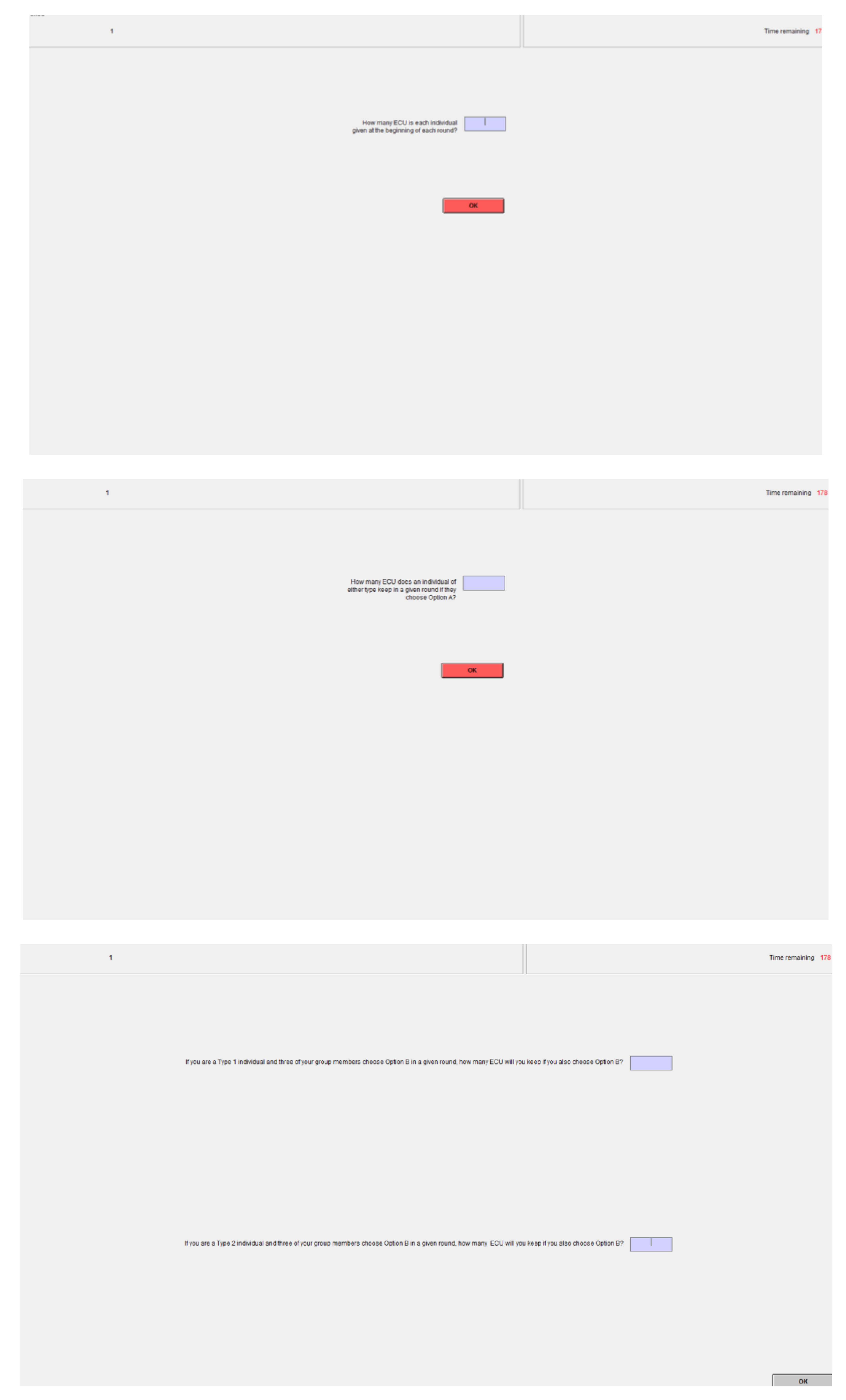

Experimental instructions (presented by experimenter):
No talking. If you have any questions after reading the instructions, please raise your hand. Your questions will be answered privately.
The experiment will last one to two hours. You are free to leave at any point during the experiment, but if you leave before the end of the experiment, you will only receive the show-up payment.
You will receive a show-up payment of $5. Your additional earnings will be based on your performance in the experiment.
You will make choices in two sequences consisting of ten rounds each. Your earnings will be equal to the sum of your earnings in each round of each sequence.
For each sequence, you will be randomly assigned to a group of six people. Your group will remain the same within a sequence, but you will be randomly reassigned to a new group at the beginning of the second sequence.
Your cash earnings will depend on your decisions and the decisions of the five other members of your group.
All decision environments are described in terms of Experimental Currency Units (ECU). At the end of the experiment you will be paid in cash at a rate of $0.08/ECU.
Sequence 1:
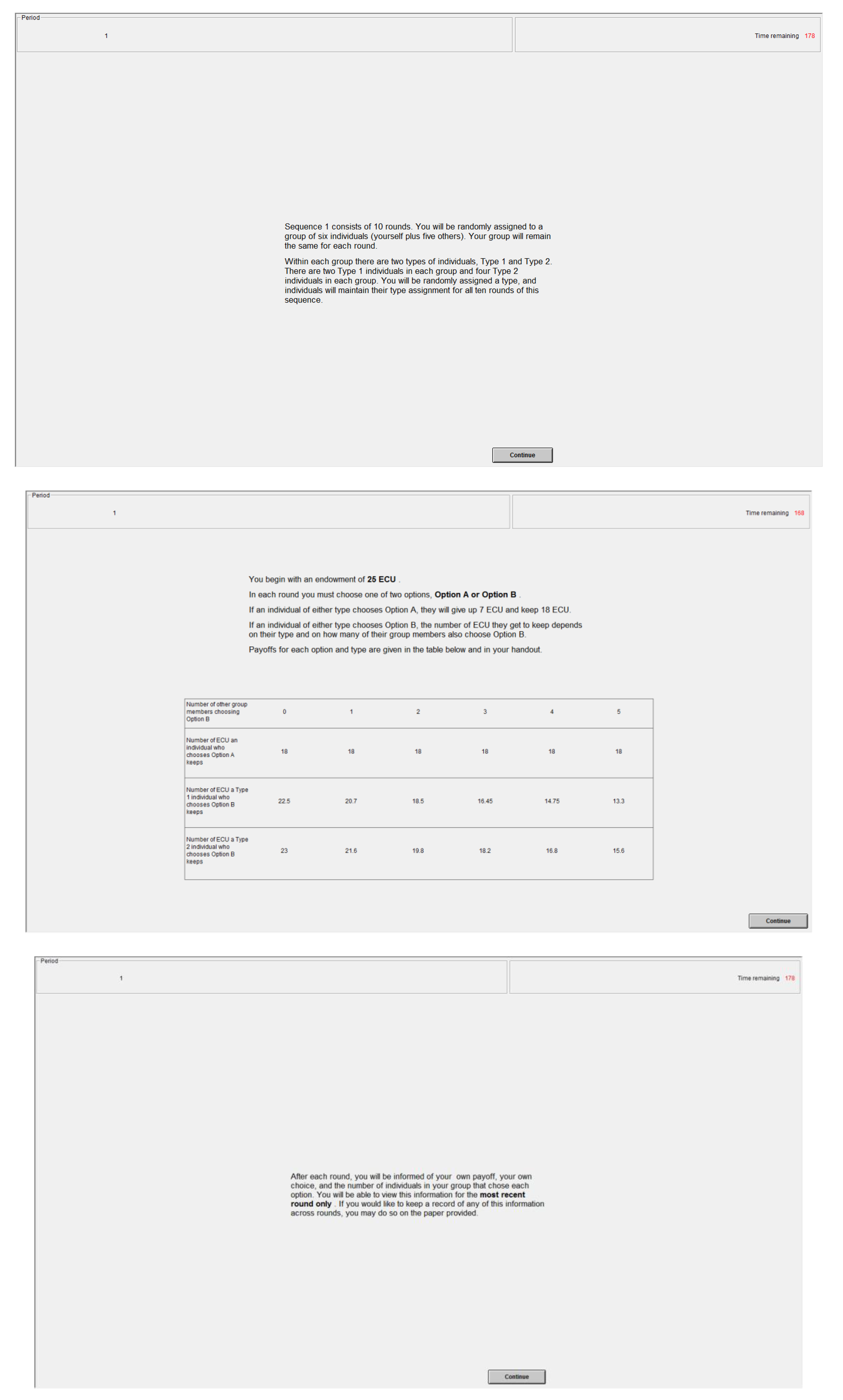
Sequence 1 consists of 10 rounds. You will be randomly assigned to a group of six individuals (yourself plus five others). Your group will remain the same for each round.
Within each group, there are two types of individuals, Type 1 and Type 2. There are two Type 1 individuals in each group and four Type 2 individuals in each group. You will be randomly assigned a type, and individuals will maintain their type assignment for all ten rounds of this sequence.
You begin with an endowment of _____ ECU.
In each round you must choose one of two options, Option A or Option B.
If an individual of either type chooses Option A, they will give up 7 ECU and keep 18 ECU. If an individual of either type chooses Option B, the number of ECU they give up and get to keep depends on their type and on how many of their group members also choose Option B.
Payoffs for each option and type are given in the table below and in your handout (25 ECU endowment payoff table or 7 ECU endowment payoff table).
After each round you will be informed of your own payoff, your own choice, and the number of individuals in your group that chose each option. You will be able to view this information for the most recent round only. If you would like to keep a record of any of this information across rounds, you may do so on the paper provided (After the end of sequence 1, sequence 2 instructions were presented, and sequence 2 payoff table handouts were distributed. Sequence 2 instructions were identical to the above sequence 1 instructions, except with the other endowment level).
References
- Andreoni, J. Warm-glow versus cold-prickle: The effects of positive and negative framing on cooperation in experiments. Q. J. Econ. 1995, 110, 1–21. [Google Scholar] [CrossRef]
- Park, E. Warm-glow versus cold-prickle: A further experimental study of framing effects on free-riding. J. Econ. Behav. Organ. 2000, 43, 405–421. [Google Scholar] [CrossRef]
- Sonnemans, J.; Schram, A.; Offerman, T. Public good provision and public bad prevention: The effect of framing. J. Econ. Behav. Organ. 1998, 34, 143–161. [Google Scholar] [CrossRef]
- Cox, C. Decomposing the effects of negative framing in linear public goods games. Econ. Lett. 2015, 126, 63–65. [Google Scholar] [CrossRef] [Green Version]
- Thaler, R.; Johnson, E. Gambling with the house money and trying to break even: The effects of prior outcomes on risky choice. Manag. Sci. 1990, 36, 643–660. [Google Scholar] [CrossRef]
- Rosenboim, M.; Shavit, T. Whose money is it anyway? Using prepaid incentives in experimental economics to create a natural environment. Exp. Econ. 2012, 15, 145–157. [Google Scholar] [CrossRef]
- Davis, L.R.; Joyce, B.P.; Roelofs, M.R. My money or yours: House money payment effects. Exp. Econ. 2010, 10, 171–178. [Google Scholar] [CrossRef]
- Cherry, T.L.; Frykblom, P.; Shogren, J.F. Hardnose the dictator. Am. Econ. Rev. 2002, 92, 1218–1221. [Google Scholar] [CrossRef]
- Oxoby, R.J.; Spraggon, J. Mine and yours: Property rights in dictator games. J. Econ. Behav. Organ. 2008, 65, 703–713. [Google Scholar] [CrossRef]
- Reinstein, D.; Riener, G. Decomposing desert and tangibility effects in a charitable giving experiment. Exp. Econ. 2012, 15, 229–240. [Google Scholar] [CrossRef]
- Etchart-Vincent, N.; L’Haridon, O. Monetary incentives in the loss domain and behavior toward risk: An experimental comparison of three reward schemes including real losses. J. Risk Uncertain. 2011, 42, 61–83. [Google Scholar] [CrossRef] [Green Version]
- Sorensen, A. Asymmetry, uncertainty, and limits in a binary choice experiment with positive spillovers. J. Econ. Behav. Organ. 2015, 116, 43–55. [Google Scholar] [CrossRef]
- Kahneman, D.; Tversky, A. Prospect Theory: An Analysis of Decision under Risk. Econometrica 1979, 47, 263–291. [Google Scholar] [CrossRef]
- Erev, I.; Eyal, E.; Roth, A. A choice prediction competition for market entry games: An introduction. Games 2010, 1, 117–136. [Google Scholar] [CrossRef] [Green Version]
- Greiner, B. An Online Recruitment System for Economics Experiments. In Forschung und Wissenschaftliches Rechnen; Kremer, K., Macho, V., Eds.; Gesellschaft für wissenschaftliche Datenverarbeitung: Göttingen, Germany, 2004; pp. 79–93. [Google Scholar]
- Fischbacher, U. z-tree: Zurich toolbox for ready-made economics experiments. Exp. Econ. 2007, 10, 171–178. [Google Scholar] [CrossRef]
| 1 | The game in [12] was motivated by the individual vaccination decision, with Option A representing a choice to receive a costly but fully effective vaccine, and Option B representing a choice not to vaccinate and potentially get sick, with one’s likelihood of getting sick increasing with the number of unvaccinated individuals. |
| 2 | and are as in [12], and were determined by a more complex probabilistic contagion model in which the application of interest was individual vaccination decisions. |
| 3 | For sequence 2 columns, the round number corresponds to the round within that sequence. That is, “Round 1” is technically the 11th round in the session, “Round 2” is the 12th round, and so on. |
| 4 | This general pattern of individuals choosing Option A more often when e = 25 than when e = 7 in early rounds only is consistent across subject types (High-loss and Low-loss). |
| 5 | In the actual experiments, High-loss subjects were referred to as “Type 1” and Low-loss subjects were referred to as “Type 2”. Subjects knew their own type and the distribution of types within their group. |
| 6 | This was done to encourage subjects to treat each round within a sequence as the same decision task, beginning with an endowment of either 25 ECU or 7 ECU, instead of with their prior earnings or losses built into the next round’s endowment. |
| 7 | Complete experimental instructions and screenshots are included in Appendix. |
Figure 1.
Proportion “Option A” by round and endowment level.


Table 1.
Payoffs by type and option choice for endowment = 25.
| Number of Other Agents who Choose Option B | ||||||
|---|---|---|---|---|---|---|
| 0 | 1 | 2 | 3 | 4 | 5 | |
| Option A Payoff | 18 | 18 | 18 | 18 | 18 | 18 |
| High-loss, Option B payoff | 22.50 | 20.70 | 18.50 | 16.45 | 14.75 | 13.30 |
| Low-loss, Option B payoff | 23.00 | 21.60 | 19.80 | 18.20 | 16.80 | 15.60 |
Table 2.
Payoffs by type and option choice for endowment = 7.
| Number of Other Agents Who Choose Option B | ||||||
|---|---|---|---|---|---|---|
| 0 | 1 | 2 | 3 | 4 | 5 | |
| Option A Payoff | 0 | 0 | 0 | 0 | 0 | 0 |
| High-loss, Option B payoff | 4.50 | 2.70 | 0.50 | −1.55 | −3.25 | −4.70 |
| Low-loss, Option B payoff | 5.00 | 3.60 | 1.80 | 0.20 | −1.20 | −2.40 |
Table 3.
Proportion “Option A” by endowment level, sequence order, and round.
| e = 25 (S1) | e = 7 (S1) | e = 25 (S2) | e = 7 (S2) | |
|---|---|---|---|---|
| Round 1 | 0.40 | 0.13 | 0.60 | 0.33 |
| Round 2 | 0.50 | 0.50 | 0.33 | 0.20 |
| Round 3 | 0.40 | 0.23 | 0.40 | 0.27 |
| Round 4 | 0.33 | 0.43 | 0.37 | 0.40 |
| Round 5 | 0.43 | 0.37 | 0.47 | 0.47 |
| Round 6 | 0.43 | 0.43 | 0.43 | 0.47 |
| Round 7 | 0.43 | 0.37 | 0.43 | 0.37 |
| Round 8 | 0.40 | 0.37 | 0.43 | 0.37 |
| Round 9 | 0.43 | 0.40 | 0.47 | 0.47 |
| Round 10 | 0.30 | 0.47 | 0.43 | 0.43 |
| All rounds | 0.41 | 0.37 | 0.44 | 0.38 |
| Rounds 1–5 | 0.41 | 0.33 | 0.43 | 0.33 |
| Rounds 6–10 | 0.41 | 0.41 | 0.44 | 0.42 |
Table 4.
Logistic regression results.
| Endowment | Sequence | Type | Constant | |
|---|---|---|---|---|
| All rounds | 0.276 * (0.145) | 0.033 (0.145) | 2.180 *** (0.184) | −1.497 *** (0.200) |
| Round 1 | 1.312 *** (0.425) | 1.003 ** (0.421) | 0.977 ** (0.434) | −2.134 *** (0.465) |
| Round 2 | 0.314 (0.398) | −1.068 *** (0.403) | 0.955 ** (0.415) | −0.470 (0.359) |
| Round 3 | 0.710 * (0.403) | 0.799 (0.400) | 0.686 * (0.413) | −1.393 *** (0.401) |
| Round 4 | −0.333 (0.410) | 0.000 (0.409) | 1.729 *** (0.422) | −0.939 ** (0.380) |
| Round 5 | 0.172 (0.415) | 0.343 (0.416) | 2.086 *** (0.446) | −1.235 *** (0.400) |
| Round 6 | −0.078 (0.396) | 0.078 (0.396) | 1.637 *** (0.421) | −0.789 ** (0.369) |
| Round 7 | 0.420 (0.462) | 0.000 (0.458) | 2.799 *** (0.489) | −1.610 *** (0.446) |
| Round 8 | 0.305 (0.453) | 0.102 (0.451) | 2.638 *** (0.474) | −1.597 *** (0.440) |
| Round 9 | 0.088 (0.419) | 0.263 (0.419) | 2.216 *** (0.456) | −1.149 *** (0.398) |
| Round 10 | −0.484 (0.444) | 0.291 (0.442) | 2.517 *** (0.472) | −1.162 *** (0.407) |
*** denotes significance at the 99% confidence level; ** denotes significance at the 95% confidence level; * denotes significance at the 90% confidence level; standard deviations in parentheses.
© 2018 by the author. Licensee MDPI, Basel, Switzerland. This article is an open access article distributed under the terms and conditions of the Creative Commons Attribution (CC BY) license (http://creativecommons.org/licenses/by/4.0/).
Share and Cite
MDPI and ACS Style
Sorensen, A. Creating a Domain of Losses in the Laboratory: Effects of Endowment Size. Games 2018, 9, 13. https://doi.org/10.3390/g9010013
AMA Style
Sorensen A. Creating a Domain of Losses in the Laboratory: Effects of Endowment Size. Games. 2018; 9(1):13. https://doi.org/10.3390/g9010013
Chicago/Turabian StyleSorensen, Andrea. 2018. "Creating a Domain of Losses in the Laboratory: Effects of Endowment Size" Games 9, no. 1: 13. https://doi.org/10.3390/g9010013
Note that from the first issue of 2016, this journal uses article numbers instead of page numbers. See further details here.