Sequential Auctions with Capacity Constraints: An Experimental Investigation


1
Departamento de Economía Aplicada I, Universidad Rey Juan Carlos, Paseo Artilleros s/n, 28032 Madrid, Spain
2
Department of Economics, University of Southern California, 3620 South Vermont Ave. Kaprielian (KAP) Hall, 300 Los Angeles, CA 90089-0253, USA
*
Author to whom correspondence should be addressed.
Games 2018, 9(1), 15; https://doi.org/10.3390/g9010015
Submission received: 13 November 2017
/
Revised: 19 February 2018
/
Accepted: 28 February 2018
/
Published: 12 March 2018
Abstract
:We conduct a laboratory experiment where groups of 4 subjects constrained to obtain at most one good each, sequentially bid for three goods in first and second price auctions. Subjects learn at the beginning of each auction their valuation for the good and exit the auction once they have obtained one good. We show that, contrary to equilibrium predictions, subjects’ bidding behavior is excessively similar across units and across mechanisms at the aggregate level. We provide two (complementary) explanations for these departures. One is bounded rationality. Subjects do not fully comprehend subtle differences between mechanisms. The other is self-selection. Subjects are very heterogeneous and some of them deviate more from equilibrium than others. Since deviations take mostly the form of overbidding, these subjects win the first or second good and exit the auction, leaving those who play closer to theoretical predictions to bid for the third good. Support for this hypothesis comes from the documented higher bidding, lower efficiency and lower profits associated with the first and second unit compared to the third one.
1. Introduction
Bidding behavior in auctions has long been studied from an experimental perspective under different environments, such as private values, common values and affiliate values, and using different mechanisms, such as first-price, second-price, all-pay, English and Dutch (see [1] for a recent detailed survey). Most of the literature has focused on single unit auctions. In this paper, we are interested in studying sequential auctions in which bidders fulfill their needs once they have obtained one good and drop out of the market for subsequent ones. These are auctions with capacity constraints, since obtaining a good saturates the capacity of the participant for a time, restricting the possibility to bid in an auction. In a recent survey, they are called “multi-unit auctions with single-unit demand” [2].
There also exists some research studying sequential auctions. It concentrates mainly on buyers bidding for identical goods (condos, wine, roses). The empirical literature [3,4,5] has emphasized a “decreasing price anomaly”: contrary to the theoretical prediction [6], the price for identical goods drops in later auctions. Heterogeneity in risk aversion can account for this pattern [7]. The same anomalous behavior is observed in a controlled laboratory experiment [8]. Following the theoretical argument in [7], the authors classified subjects according to their degree of risk aversion. These results are replicated using an English auction in [9]. Patience or “wait-and-see” strategies have also been analyzed under the same experimental rules in [10], with the addition of uncertainty in the number of goods supplied. Finally, two consecutive first-price auctions with two bidders who can undertake only one project each have been studied [11]. In all this literature, however, valuations for all goods are known at the outset.
In this paper, we are interested in a related but different paradigm. We study the behavior of individuals in sequential auctions where the valuation for a good is drawn after the allocation of the previous one. Real-life situations of this sort abound. Construction companies submit bids for building a major infrastructure. They know their cost and the potential benefit of being the awardee, but they also know that there will be other procurement contracts in the future, and that once a contract is awarded their limited capacity may prevent them from bidding in others. A similar trade-off arises for transportation companies with reduced fleets and suppliers of raw materials. A key property of these situations is that some contracts are a better fit than others. For example, the construction company may be better suited to handle a large residential project in a steep rural landscape than a medium-size commercial project in an urban area. Similarly, the transportation company may be better equipped for a small number of long haul drives than a large number of short ones. This means that, while the specific characteristics of the current contract are known at the timing of bidding, the value of the possible future contracts is not.
This dynamic assignment problem is characterized by a subtle intertemporal trade-off between current payoffs and future options. The singularity of the situation is that bidders have information about the current good but uncertainty about the future ones, not knowing which type of good will be auctioned next. The aim of our paper is to study this trade-off in a controlled laboratory setting given different allocation mechanisms. We are interested in determining the empirical bids across mechanisms and compare them to the theoretical predictions. More importantly, we want to find out if subjects realize that patience pays off. Indeed, in our setting, winning good t prevents subjects from bidding for good t + 1, which other things being equal makes good t less desirable. In other words, there is an option value of waiting—very much on the lines of the literature on investment under uncertainty [12]—which implies that, for a given valuation, bids should be lower and profits higher for goods auctioned early compared to goods auctioned late. Whether our participants realize this dynamic effect and bid accordingly is the main question we want to address.
To the best of our knowledge, there is only one existing set of sequential auction experiments where valuations for a good are drawn after the allocation of the previous one [13,14] are. The authors study a two-good setting with synergies, where the agent who obtains the first good has an increased valuation for the second good. As a result, there is an incentive to overbid for the first good and capitalize with the second. The authors find that subjects face an exposure problem and do not fully incorporate in their bid the extra value of winning. Our paper shares the sequential revelation of valuations but focuses on the opposite inter-temporal trade-off since, as noted above, the larger option value of waiting in the early rounds induces an incentive to amplify bid shading.
Formally, our experiment has groups of 4 subjects sequentially bidding for 3 goods, both under the rules of first- and second-price sealed bid auctions. Valuations are provided to the subjects “one-at-a-time”, and the winner of a good cannot bid for the remaining one(s). Theory predicts lower bids for earlier goods due to the “option value of waiting” mentioned above and for first-price auctions relative to second-price auctions due to the obvious effect of higher payments conditional on bids.
Not surprisingly considering the existing literature auctions (see [1,15] for reviews), we find that subjects in our experiment deviate from the theoretical predictions, with an overall tendency to bid above the risk neutral Nash equilibrium in first-price auctions and above the dominant strategy in second-price auctions. Subjects also exhibit a qualitatively similar bidding behavior across mechanisms. Even though bids are higher in second-price than in the first-price auctions, the contribution of values to bids (slope) is similar across mechanisms. Finally, and perhaps more interestingly, we find similar bidding behavior across goods, implying more overbidding in earlier than in later auctions under both mechanisms.
The similarity in bidding across auctions suggests an imperfect understanding of distinctions across mechanisms. The similarity in bidding across goods can be also due to an imperfect understanding of the option value effect. However, it may be the result of a subtler dynamic self-selection effect. Indeed, subjects with a tendency to overbid are likely to win early goods (1 and 2) and exit the auction, leaving only those who play close to equilibrium or underbid competing for the last good (3). If this hypothesis is correct, we should then observe that subjects who typically win good 3 bid closer to equilibrium for all goods than subjects who typically win goods 1 and 2, and also make higher profits. Overall, when competing against irrational bidders, patience (that is, waiting until the over-bidders get a good and leave the auction) pays off.1
Interestingly, our results support the self-selection hypothesis. Indeed, for each mechanism, subjects overbid less and earn more in the last good than in the first good. We then divide subjects into those who often win goods 1 and 2 (early winners) and those who often win good 3 or none of them (late winners). An analysis of the bidding behavior suggests that early winners overbid substantially more than late winners not only for goods 1 and 2 (which explains why they win them so often) but also for good 3. We also show that the average efficiency is much larger for good 3 than for goods 1 and 2, mostly because of a change in the composition of the population: our irrational bidders (who overbid and “steal” the good despite their not having the highest valuation) obtain goods 1 and 2 and leave the subjects who bid closest to equilibrium compete for good 3. In other words, even though early winners also overbid whenever they reach good 3, the efficiency is high simply because they rarely reach good 3. Finally, the same change in the composition of the population implies that patience pays off: late winners obtain substantially higher profits than early winners and gains are larger in the last good than in the first two, even though the theoretical prediction is the opposite.
Finally, it is interesting to notice that a substantial fraction of irrational over-bidders remain in the auction after the allocation of the first good, as witnessed by the remarkably similar levels of high overbidding, low efficiency and low payoffs in goods 1 and 2. In other words, removing the 25% of subjects who win good 1 is not enough to significantly reduce the departures from equilibrium. Efficiency is significantly improved and overbidding significantly reduced only after 50% of subjects have left the auction.
Notice that the result is analogous to the well-documented decreasing price anomaly discussed above. Indeed, with identical goods the theory predicts constant prices (on average) whereas the laboratory experiments exhibit declining prices. Since in our setting the theory predicts increasing prices, observing constant prices is consistent with the bias in that literature.2 This means that, instead of self-selection, the risk-aversion explanation proposed in [7] and tested in [8] could potentially explain the behavior of our subjects. While we do not have enough data to test and disentangle between these two theories, the fact that our most aggressive subjects make very small or even negative profits in the auctions of the first and second goods suggests that only implausible levels of risk aversion could justify their behavior.
The paper is organized as follows. In Section 2, we develop the theory of dynamic bidding in first- and second-price auctions together with a description of the hypotheses. In Section 3, we describe the experimental design. In Section 4, we perform an aggregate analysis and study the bidding functions, efficiency and payoffs by good and mechanism. In Section 5, we conduct a cluster analysis and test our self-selection hypothesis to explain the differences in bidding, efficiency and profits across goods. In Section 6, we provide some concluding comments. Proofs and a sample of the instructions and quiz are relegated to the appendix.
2. Theory
Consider the following auction setting. There are T + 1 risk-neutral bidders and T periods. In period 1, each bidder i learns his valuation for the good to be auctioned in that period. We assume that valuations are independently drawn from the distribution G(.) with support []. Each bidder i simultaneously submits a sealed-bid and the good is allocated according to the rules of mechanism M ∈ {F, S}, where F is a first-price sealed bid auction with no reserve price (highest bidder wins and pays his bid) and S is a second-price sealed-bid auction with no reserve price (highest bidder wins and pays the second highest bid). The winner of the auction obtains the good and exits the auction. The T losers move to period 2 where new valuations are drawn for those bidders (independently both across bidders and across periods) from the same distribution G(.) and a new auction takes place under the same mechanism (F or S) as the previous one. The process continues until period T, the last period, where valuations are drawn for the two remaining bidders who then bid for the last remaining good.
This dynamic auction has two characteristics that we want to emphasize. First, each bidder is interested in at most one good: once they have won a good, they exit the auction and the game ends for them. This occurs in practice when the opportunity cost of obtaining a second good is prohibitively high. Second, bidder i’s valuation for good t + 1 is unknown in period t. In terms of the examples mentioned in the introduction, one can think of the owner of one truck, one taxi or one construction crew who learns and bids for jobs as they appear. Once a job has been secured, he does not have the means to bid for a second one.
Propositions 1 and 2 characterize the symmetric Bayesian Nash equilibrium of the game for bidder i (∈ {1,…, T + 1}) in period t (∈ {1,…, T}), under the first-price (F) and the second-price (S) auction mechanisms, and assuming risk-neutrality (proofs can be found in Appendix A).
Proposition 1.
In a first-price auction (F), the unique symmetric equilibrium bidding function of bidder i with valuation in period t, , and his equilibrium utility, , are:
where
Proposition 2.
In a second-price auction (S), the unique symmetric equilibrium bidding function of bidder i in period t, , and his equilibrium utility, , are:
where
The results are extensions of the standard one-shot first-price and second-price sealed bid auctions with no reserve price. Indeed, in the first-price auction, we can interpret VFt+1 as the value for a bidder at period t of not winning the current auction and, instead, moving to period t + 1. In the standard auction, this is nil, which is why the value of not winning the auction in the last period (T), VFT+1, is zero. At every other period t (< T), VFt+1 is positive and larger the greater the number of periods left (as we can see from (2), VFt > VFt+1). Notice also that VFt+1 is a constant, reflecting the fact that at period t bidder i does not know his future valuations.
Seen under this light, the equilibrium bid in the first-price auction at period t, btF(vi), takes a familiar form. The first two terms correspond to the static equilibrium bid when the bidder faces T + 1-t rivals, and the last term reflects the opportunity cost of winning. In other words, bidder i shades his bid relative to his valuation for two reasons: first to optimize the standard trade-off between probability of winning and net gain conditional on winning, and second to reflect the positive value of moving to period t + 1 and participating in a new auction. The equilibrium utility at period t, uitF(vi), is also familiar. It simply corresponds to the standard expected utility of a bidder in a first-price auction against T + 1-t rivals to which we add VFt+1, the value of moving to the next period.3
The analysis of the second-price auction is analogous. If in a symmetric static equilibrium subjects bid their valuation, in our problem they decrease that bid by VSt+1, the option value of moving to t + 1. and so is the expected value of moving to the next period (VFt+1 = VSt+1).
From Equations (2) and (4) it is immediate to see that VFt+1 = VSt+1, which itself implies that . In other words, and just like in the one-shot auctions, the expected payoff of bidders in each period is identical across mechanisms. Combining (1) with (2) and (3) with (4), the utility in period t can be rewritten as:
This means that uitF(vi) > uit+1F(vi) and uitS(vi) > uit+1S(vi) for all t and G(.): as we move from one period to the next, the expected utility of a subject decreases, simply because he faces fewer options to obtain a good.
Notice that the analysis assumes no reserve price, which we know is suboptimal from the seller’s viewpoint. Determining the equilibrium with optimal reserve price poses no extra difficulty. Remember, however, that the objective is not to find optimal mechanisms but to build a simple framework that we can export to the laboratory. We therefore opted for an environment with no reserve price.
Finally, suppose that a subject with valuation vi wins the auction at date t. His utility in the first-price auction is then (which, by the equivalence of the mechanisms, is also equal to his expected utility in the second-price auction). From an ex-ante perspective, , the expected payoff of the winner at t is:
One can check that . The expected payoff of the winner decreases over periods for two reasons. First, because bids increase with t and therefore the net gain of the winner decreases with t. Second, because as t increases, the number of bidders decreases. By the largest order-statistics, this means that the distribution of the highest valuation (which in equilibrium is the valuation of the winner) shifts towards lower values.
We next develop the simple numerical example that will be used in our experiment.
Numerical Example.
Suppose that , and T = 3, we get:
- VF1 = VS1 = 18; VF2 = VS2 = 15; VF3 = VS3 = 10; VF4 = VS4 = 0.
- u1F(vi) = u1S(vi) = ; u2F(vi) = u2S(vi) = ; u3F(vi) = u3S(vi) = .
- b1F(vi) = ; b2F(vi) = ; b3F(vi) =
- b1S(vi) = ; b2S(vi) = ; b3S(vi) = .
- ; ; .
We can use these bidding functions to formalize theoretical predictions of equilibrium behavior by risk neutral bidders. The predicted differences across mechanisms and across periods will then be tested with the data of our experiment.
Prediction 1.
At each period t and for a given valuation , bidding is lower but the utility of the winner is the same in the first-price than in the second price auction.
Prediction 2.
In each mechanism M {F, S}) and for a given valuation , bidding is lower and the utility of the winner is higher in period 1 than in period 2 and in period 2 than in period 3.
3. Experimental Design and Procedures
We conducted four sessions with 12 subjects and two sessions with 16 subjects for a total of 80 participants. All sessions were held at a computer lab in the Vicálvaro Campus of the Universidad Rey Juan Carlos (URJC) in Madrid (Spain). Subjects were recruited via email after posting a message on the university website calling for participation on a seminar about auctions but without any notification neither that the experiment was going to be held nor that they were going to get paid. Subjects who showed up were informed about the experiment and were given the option to withdraw. All decided to participate.
In each session, subjects had to bid on eight rounds according to the rules of a first-price (F) or a second-price (S) auction. To control for order effects, in three sessions subjects started with four rounds of F followed by four rounds of S whereas in the other three sessions the order was reversed.
At the beginning of each round, subjects were randomly and anonymously matched into groups of 4. Subject knew about the procedures but did not know the identity of the subjects they were matched with.
For each group and each round, the auction consisted of the allocation of three goods to the four subjects in the group, with three subjects obtaining one good each and the other subject obtaining none. The allocation mechanism followed closely the procedure described in Section 2. When the first good was auctioned (from now on G1), all 4 subjects in the group received a random valuation for that good (and not for the other two to come). After sealed bidding, G1 was assigned to the highest bidder and the awarded price was the highest bid (F) or second highest bid (S), depending on the mechanism being used. The winner of the auction could not bid anymore in that round. Valuations were then drawn for the second good (from now on G2) for the remaining 3 subjects. Once again, G2 was awarded according to the same mechanism (F or S) and the winner was withdrawn. Finally, for the third good (from now on G3), the last one, only two subjects remained. They both bid for the good and one got it while the other finished the round with no good.4
Valuations for each good in each round were denominated in tokens. All valuations were privately and independently drawn randomly from a uniform distribution in [30,90]. Bids were constrained to the range (0,150], rounded to 2 decimal places. For each good in each round, the payoff of the winner was value minus own bid (F) or value minus second highest bid (S). The profit of the loser(s) and the subject(s) not bidding (i.e., those who won a previous good in that round) was 0.
At the end of the session, the subjects were paid according to one round that was chosen at random by throwing three coins and showing the resulting sequence of heads and tails to the participants. The payoff was converted to euros at a ratio of 1 euro per four tokens. Subjects also earned a show-up fee of 2 euros.5
The timing of the experiment was the following. First, the experimenter read the instructions (see Appendix B for a sample copy of the English translation) showing sample screenshots in an overhead projector. Then, subjects took a comprehension quiz on paper to make sure they had completely understood the instructions (see Appendix C for a sample copy of the English translation). After that, subjects went through one practice round that did not count for the final payoff and then they participated in the 8 paid rounds of the experiment. Finally, the subjects were paid in cash and in private their total earnings. Sessions averaged 75 min and subjects’ earnings averaged 5.6 euros, which is admittedly low for the standards in economics experiments.6
For each round and group, nine bids were submitted: 4 bids for G1, 3 for G2 and 2 for G3. Since there were 80 participants in the experiment, there were a total of 20 groups, each playing eight rounds. The total number of bids was 640 for G1, 480 for G2 and 320 for G3, of which half corresponded to mechanism F and the other half to S. The experiment was programmed and conducted with the software z-Tree [17].
Ethics Statement.
The experiment falls in the category of non-medical behavioral experiments in social sciences. It was run with IRB approval from USC (# UP-08-00052) and consent of the ethical committee of URJC.
4. Aggregate Results
4.1. Summary Statistics
We start with some indicators that summarize the main features of the experiment, looking at goods and mechanisms separately.
The first indicator relates to the efficiency of the auctions (Table 1). We consider two measures. One measure is the percentage of times the good is allocated to the subject with the highest valuation (Allocation Efficiency). The efficiency is similar for G1 and G2 and increases substantially for G3. S auctions are generally more efficient, although it is surprising to see that the efficiency for G2 is lowest. The efficiency for F auctions is always increasing. Note that an increase in efficiency over auctions can be partly attributed to the decrease in the number of bidders (for instance, random allocation would predict efficiencies of 25%, 33% and 50% in G1, G2 and G3). The 90% allocation efficiency of G3 is high but in line with early studies [18,19].7 As we will see all along the paper, differences across goods are partly due to the endogenous “exit” (through winning) of subjects. Another measure of efficiency is the surplus obtained relative to the maximal attainable surplus in each round of each auction (Surplus Efficiency).8 As we can see from Table 1, once we correct for severity, efficiency measures are high and similar across all goods and auction formats.
The second indicator is the payoff obtained by the winner in each mechanism and for each good, defined as the average of the valuation of the winner minus bid (F) or the average of the valuation of the winner minus second highest bid (S) (Table 2). It also shows the theoretical prediction, as described in Equation (6) and applied to our numerical example. Negative empirical values indicate paying a price over one’s own value when winning. Differences from theory occur for two main reasons. First, overbidding results in smaller gains conditional on winning. Second, it may also imply stealing the good, that is, winning when another subject has a higher valuation. This means a non-zero rather than zero payoff for that subject but an overall loss in surplus.
There is a high dispersion in payoffs in both auctions. We also notice large payoffs differences between mechanisms with statistically significant profits in S (although well below equilibrium in G1 and G2) and profits not significantly different from zero in F, despite the identical theoretical prediction (Prediction 1). A possible explanation is that if only the winner bids above value, he will incur in losses in F but not in S, where the price is determined by the second highest bid. In other words, irrationality of a fraction of subjects is likely to be costlier in F than in S. Last and perhaps most interestingly, payoffs increase between G2 and G3. This is in sharp contrast with the theoretical predictions, where the increasing bids and the lower continuation value as we move from G1 to G3 imply decreasing expected profits of the winner (Prediction 2). As we develop below, the composition of subjects in G3 is different, which may be responsible for this effect.
The third indicator shows significant irrationality in some players. This is most evident from the non-negligible number of observations (around 20%) in which subjects bid over their valuation in F, invariably yielding negative payoffs in case of winning (Table 3). In those cases of overbidding, the median and mean differences between bid and valuation are smallest in G3. After removing the extreme outliers, the mean and median become very small in G3 (around 5 and 3, respectively). This irrational behavior is puzzling and substantially more prevalent than in the existing literature. A possible reason is that, unlike most of the literature, we do not prevent or explicitly discourage participants to bid above their valuation.9
4.2. Aggregate Bidding Functions
An analysis of interest consists in determining the empirical bidding behavior as a function of the valuation drawn by the subject. For the remaining of the paper, we refer to “overbid” as the difference between the experimental bid and the (unique symmetric) risk-neutral equilibrium bid predicted by theory (Nash). Positive values indicate overbidding and negative values underbidding. Bidding is studied by comparing theoretical predictions and experimental behavior at the aggregate level.
Figure 1 describes bidding as a function of valuation. From left to right, the first graph includes the six theoretical bidding functions (BF) derived in the numerical example of Section 2 (goods G1, G2, G3 under mechanisms F and S). Note that the equilibrium bidding functions are linear in valuation because the distribution is uniform. The second graph shows the empirical bidding functions. The x-axis represents valuations. To smooth out the empirical functions, we group valuations in bins of 5 units, starting at the minimum of 30 and ending at the maximum of 90 (so 30 to 35, 35.01 to 40, etc.). The y-axis shows the average bids that correspond to all the valuations included in that bin. The third graph depicts the regression-based experimental bidding functions. Since the theoretical bidding function is linear, we use the following OLS regression to estimate the best fit of the empirical bidding functions:
where i denotes the individual, g ∈ {G1, G2, G3} the good and m ∈ {F, S} the allocation mechanism. To account for the fact that each subject bids multiple times, we compute robust standard errors clustered at the individual level. This estimate can then be compared to the theoretical ones.
Table 4 below includes the slopes and intercepts (at the minimum valuation of v = 30) of the theory and the OLS regression with their corresponding robust standard errors. It also includes the results of a t-test of comparison between the two.
Graphically, the theoretical bidding behavior shows differences between goods and mechanisms (lower bids in earlier goods and F auctions, see Predictions 1 and 2) whereas the aggregate experimental functions look similar (though not identical) across goods and mechanisms.10 This is consistent with the winner’s payoff data: the higher relative overbidding in F and in G1–G2 results in lower profits in those treatments.
Our test of comparison between theory and data corroborates those findings. There is consistent overbidding as witnessed by the higher empirical intercept in G1 and G2 under both mechanisms. This finding is consistent with the existing literature, which reports higher bids than risk neutral Nash predictions in F auctions and bids above value on average in S auctions [1,15].
Subjects are also significantly more responsive to changes in valuation than predicted by theory in F, where all the empirical slopes are above 0.9, while the theoretical are between 0.5 and 0.75. These slopes are higher but not excessively far from those reported in the literature, which are typically between 0.8 and 0.9 [22,30] and sometimes as high as 0.92 [27]. Again, our design which does not explicitly warn subjects against overbidding, may be partially responsible for the difference. Finally, notice that the slopes in G1 and G3 (but not in G2) are marginally significantly lower than 1 (p-values < 0.055). By contrast, slopes in S are not significantly different from theory in G1 and G2 and smaller than theory in G3.
To be able to better compare across goods and mechanisms, we conduct a robust regression analysis of the bid on the Value (whose coefficient captures the slope of the bidding function) a Constant (whose coefficient captures the intercept of the bidding function), as well as dummy variables for the good (G2 and G3), interaction terms between those dummies and Value, as well as a dummy Order to control for order effects. Results are reported in Table 5. Errors are clustered at the individual level to account for the dependence across individual decisions. We also report in Appendix D1 a similar exercise, where we model dependence across observations within session and order of auctions (data from one session featuring a specific order is one independent observation) and within groups (data from the group formed to play the 4 rounds of a given auction in a given session is one independent observation).
Column (1) shows that in the first-price auction, subjects bid more in G2 and G3 compared to G1. Therefore, although differences in behavior across goods are not as pronounced as the theory predicts, they are still present. By contrast, little difference across goods is observed in the second price auction with perhaps the exception of slightly higher bids in G3 (Columns (3) and (4)). There is no significant interaction in either auction (Columns (2) and (4)). Finally, by comparing the coefficients across auctions, we notice that the difference between the bidding functions in F and S seems to be due to differences in intercept rather than slopes.
Running a regression on the full sample is useful to better study such differences across auction formats. For this purpose, we create a dummy variable Second to account for the auction mechanism. The results of this exercise are reported in Table 6.
When we combine both mechanisms, we notice higher bids in G2 and G3 (an effect driven by the first-price auction data) but also significantly higher bids in S than in F (Second). The differences are smaller in magnitude than predicted by theory, but still present in the data. The results also confirm that the differences between the bidding functions in F and S are due to differences in intercept (driven by the auction format and the good) rather than slopes.
4.3. Overbidding
To deepen our understanding of the differences between theoretical and empirical bidding behavior, we provide a regression analysis of the difference between the empirical and the theoretical bids (from now on called “overbid”).11 The results are presented in Table 7. If subjects followed the theory, both the Value and Constant coefficients would be 0. Overbidding occurs but takes different forms in the different mechanisms. In F, it is the result of a steeper bidding function than predicted by theory, which is reflected in the positive coefficient of Value. In S, it is due to a higher bid than optimal for all valuations, as reflected by the positive coefficient of Constant. In each mechanism, overbidding is also significantly less prevalent in later goods (G3 in F and G2 and G3 in S). Finally, the third column reveals significantly less overbidding in S than in F, although the differences are, again, small in magnitude. These results reinforce our previous findings. Indeed, the difference in the Value coefficient for overbidding between F and S is consistent with the bidding slopes that should be smaller in F than in S, but are not empirically. Similarly, the negative coefficient of Second in columns (5) and (6) indicates that overbidding is less prevalent in S than in F, that is, participants play closer to equilibrium in S than in F.
These results are consistent with the analysis of payoffs (Appendix D3). The similar (though, as we already discussed, not identical) bidding strategy in all 6 cases translates into less overbidding but also in higher profits for the winner in later auctions and in second-price auctions.
All in all, and contrary to Predictions 1 and 2, overbidding is higher in F than in S and in earlier than in later goods. However, behavior is also highly heterogeneous across subjects, with large dispersion in bids. Heterogeneity, raises an interesting selection problem in our setting: since winners of G1 and G2 do not participate in G3, the differences in departures from theory observed across goods may be due to differences in the composition of the bidding population. We address this question in more detail in the next section.
5. Cluster Analysis
5.1. Framework and Basic Statistics
The aggregate analysis shows overbidding, with a diminishing trend across goods under both mechanisms. There are (at least) two possible explanations for this trend:
Hypothesis 1. Bounded rationality.
Subjects do not differentiate enough between mechanisms and goods, choose excessively similar bidding strategies during the entire experiment.
Hypothesis 2. Self-selection.
Some subjects deviate more from equilibrium behavior than others. Since deviations take mostly the form of overbidding, these subjects win goods early in the round, leaving those who play closer to theory to bid for G3.
There are indications of both effects in the aggregate analysis. On the one hand, the overall bidding behavior is excessively similar between F and S for all goods (Table 5 and Table 6), with significant overbidding (Table 7) and a fraction of subjects in F bidding above their valuation (Table 3). This suggests that subjects have difficulties differentiating between the two mechanisms, consistent with Hypothesis 1. On the other hand, behavior is closer to theory (Table 4), efficiency is significantly higher (Table 1), and realized profits are also higher (Table 2) in G3 than in G1 and G2. This suggests a more rational and homogeneous behavior for the last good, consistent with Hypothesis 2.
If the hypothesis of self-selection holds true, we should observe that subjects who often obtain G1 or G2 overbid more than those who obtain G3 or do not obtain any good. This will partly happen by construction in G1 and G2. More interestingly, it should also occur in G3.
To study this issue, we cluster subjects by the proportion of goods they obtain “early” vs. “late or never” in the round, and analyze their behavior to determine if their bidding strategies are different. More precisely, we define two attributes for each subject: “F3 + 0” is the percentage of rounds in which the subject has participated in G3 under F (either obtaining it -3- or not -0-) and “S3 + 0” is the percentage of times in which he has participated in G3 under S. Because our subjects play each mechanism 4 times, the percentages are 0, 25, 50, 75 or 100.
We then cluster the subjects based on these two dimensions using K-means, a clustering method that partitions the observations (here subjects) in K clusters and in which each observation belongs to the cluster with the nearest mean. According to the self-selection hypothesis, we expect two main groups. Subjects who often win G1 or G2 both in F and S, which we call EARLY-EARLY or EE. Subjects who often win G3 or do not win any good both in F and S, which we call LATE-LATE or LL. There might be also some unique bidding behaviors, with aggressive bidding and therefore high chances of early winning only in F (EARLY-LATE or EL) or only in S (LATE-EARLY or LE). A 4-means cluster seems therefore a reasonable option.12
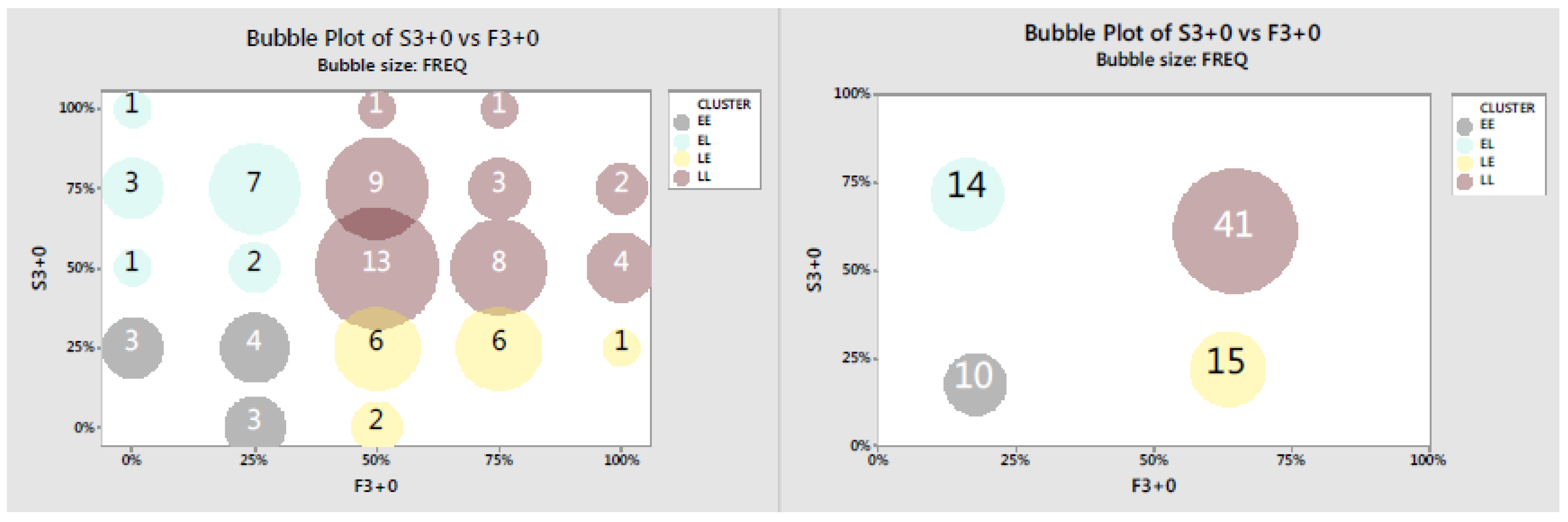
Figure 2 depicts the two-dimensional distribution of subjects, grouped in 4 clusters (the size of each circle and the number inside represent the number of subjects). Notice that our method imposes the number of clusters but not the way in which subjects should be grouped with each other. Therefore, subjects need not be clustered necessarily according to the EE, EL, LE, LL categories described above. It turns out, however, that the model naturally splits our subjects into four perfect quadrants.
The first thing to notice is that our clustering model puts in the L category the subjects who reach G3 exactly 50% of the time. Then, of the 80 participants, 41 subjects (51%) are LL, 10 subjects (13%) are EE, 15 subjects (19%) are LE, and 14 subjects (17%) are EL.13
5.2. Overbidding
We first report in Table 8 the average overbidding (difference between empirical choice and equilibrium prediction) in each good and mechanism separated by cluster.
The average overbidding of an early winner ranges from 15.9 to 30.0 whereas that of a late winner is between 3.5 and 14.2. Overall and consistent with Hypothesis 2, overbidding is more than twice as high for EE than for LL both in F and in S. Furthermore, overbidding decreases across goods, which again is consistent with Hypothesis 2 regarding the change in the composition of the population across goods. Interestingly, the decrease in overbidding is most pronounced between the second and third good, suggesting that the self-selection effect is still present after removing the 25% of subjects who substantially overbid and win the first good. Finally, notice that the difference in overbidding between EE and LL is significant not only on average but also on a good by good basis. In particular, an EE subject who reaches G3 will overbid about 13 tokens more than an LL who reaches G3. This means that overbidding is truly a characteristic of the individual and not an artifact of our classification.14 Similar tendencies are observed with EL and LE.
5.3. Efficiency
The substantial overbidding of a large fraction of the population for G1 and G2 (the “early” subjects) may hamper the efficiency of the mechanisms. Table 9 shows the allocation efficiency in F and S. It represents for each cluster whether the bidder with the highest valuation effectively won the auction (Same) or did not (Other). Columns are added to summarize efficiency across goods.
For G1 and G2 in F, efficiency is very high, whenever an “early” subject (EE or EL) has the highest valuation. These subjects also frequently steal the goods that a “late” subject (LE or LL) should obtain, which decreases dramatically the efficiency in those cases. Once we reach G3, most early subjects have already obtained a good. The presence of overbidders is not as widespread as in G1 and G2 so their competition is not as fierce, resulting in high efficiency levels. The analysis is similar in S: high efficiency in G1 and G2 when an early subject (in this case, EE or LE) has the highest valuation and much lower efficiency when a late subject (EL or LL) has the highest valuation. Again, efficiency is uniformly high in G3. These results are also consistent with Hypothesis 2 and further supported by an analysis of payoffs across clusters (see Appendix D4): early winners incur lower payoffs in both auctions.
5.4. Summary
The cluster analysis of this section suggests that two effects contribute to the insufficient distinction in bidding behavior across goods and mechanisms. First and as extensively documented in previous experiments on auctions [1], there is evidence of bounded rationality. Subjects have problems realizing the distinction between first and second price auction, and the corresponding differences in optimal bidding behavior. We show that this problem is most severe in G1 and G2 but persists in G3, despite the different composition of the subject population. Second and more interestingly, we emphasize a selection effect across goods. Subjects who obtain the good early tend to severely overbid in all goods, including the last one. They also steal goods, lowering the allocation efficiency when their type is prevalent (first and second good) but less so when their type is less common (third good).
6. Conclusions
In this paper, we have provided a simple framework to study sequential auctions with capacity constraints. We have identified a novel self-selection effect, whereby irrational overbidders obtain early good(s) and exit the auction, leaving the most rational ones (and maybe also the underbidders) competing for the late good(s). In this setting, the patience of rational bidders pays off: both the efficiency and the payoff of the winner are higher for the last good than for the first two. The setting may not be appropriate to capture markets with highly experienced bidders or markets with a continuous flow of entry and exit of bidders. By contrast, it is highly suitable for markets with a fixed number of capacity constrained, moderately experienced players.
The self-selection result raises a number of theoretical and experimental questions. First, it would be interesting to develop a behavioral theory of boundedly rational bidding in markets with capacity constraints. Indeed, mistakes are not equally costly if they take the form of under- or over-bidding. Their relative cost and the efficiency consequences are also different in first- and second-price auctions. As a result, the best response of rational bidders to this boundedly rational behavior will also depend on the composition of over- and under-bidders in the population as well as their likelihood to exit early. Second, it would be instructive to extend the framework to the case where goods are drawn from different distributions. It is a priori unclear if the departures from equilibrium behavior will be exacerbated if the stochastically “best” goods (those drawn from H(vi), with H(vi) < G(vi) for all vi) are offered early and the stochastically “worst” goods are offered late or vice versa. It also raises interesting questions for the auctioneer. Should a profit-maximizing seller start or end with the best goods? How does this depend on the fraction of over-bidders in the population? Finally, our experiment has only 8 rounds leaving little room to our subjects for learning to bid optimally. It would be interesting to determine if in an experiment with more rounds (say, 20 or 30) over-bidders learn the costs of their behavior and converge over time to the equilibrium strategy. Alternatively, it would be also interesting to train subjects in one-shot experimental auctions and then run a phase similar to the one conducted in this experiment. Such variant could help explaining why the behavior across goods and mechanisms is so similar in our setting. This and other related questions will be the object of future investigation.
Acknowledgments
We thank seminar participants at USC for comments. We also thank LUSK Center for Real State at USC and Banco de Santander-URJC for financial support.
Author Contributions
Isabelle Brocas and Juan D. Carrillo conceived and designed the experiments; F. Javier Otamendi performed the experiments; all three authors analyzed the data and wrote the paper.
Conflicts of Interest
The authors declare no conflict of interest. The founding sponsors had no role in the design of the study; in the collection, analyses, or interpretation of data; in the writing of the manuscript, and in the decision to publish the results.
Appendix A. Proofs of Propositions 1 and 2
First-price auction.
Consider period t (). Consider agent i with T − t + 1 opponents. Valuations are independently drawn from distribution G(.) in []. Agent i anticipates that agent j ≠ i bids bt(vj) where bt(.) is a monotonic increasing function (the same for all j).
Since, in period t, the valuations of periods t + 1 to T () are unknown, we can without loss of generality denote Vt+1 the (constant) expected utility of not winning the auction at t. Naturally, this value will be endogenously determined in equilibrium.
Given this notation, if i announces bi and gets the good, his surplus is vi − bi. If he does not get it, his surplus is Vt+1. The utility of i is then given by:
Bidder i chooses bi such that = 0. Differentiating with respect to vi and using the previous optimality condition, we get:
We assume that in each round one good is allocated with certainty (which is true if we impose no restrictions on bids and no reserve price). At equilibrium, never gets the good in that period. Therefore, the utility of a bidder with valuation is Vt+1. Overall,
Then, for all , the optimal bid is given by:
which means in particular that . This equilibrium implies a positive bid (> 0) as long as (in the numerical application of the experiment, we make sure that this condition is satisfied so that the non-negative bid constraint is not binding). The equilibrium utility is:
Once we know the expression of the utility at a given period t + 1, we can use it to compute Vt+1, which is simply the expectation of this utility before learning the draw :
Integrating by parts, we get:
Overall, Equation (A7) provides a recursive formulation of the expected payoff of not winning the auction at period t. Noticing that the horizon is finite (T is the last period), we can use a recursion to rewrite as:
The last step is to determine the boundary condition. By definition, = 0 since it represents the continuation payoff of not getting the good in period T (the last one). Therefore:
Inserting the continuation value from Equation (A9) into the utility from Equation (A5), we get:
Second-price auction.
The proof for the second-price auction follows a similar line (it is straightforward to see that it is a weakly dominant strategy for subject i to bid his modified valuation ). Finally, notice that both auction formats yield the same expected utility to bidders and therefore also give the same expected revenue to the seller.
Appendix B. Instructions
You15 are going to participate in an experiment in which you will have to make decisions in groups, and you will be paid in cash at the end of the experiment. Each participant may obtain different amounts due partly to its own decisions, partly due to the decisions of others, and partly due to the luck of the draws. The experiment is computer-based and all the interactions among participants will be through the PC. It is important that you do not talk and that you do not try to communicate with other participants throughout the experiments.
We will start with a short period of instructions, in which you will be instructed on the rules of the experiment, and you will be taught on how to use the computers. It is very important that you pay close attention. If any questions arise, raise your hand and the answer will be given out loud for everyone. If any doubts strike your mind, raise your hand and I will help you with the computer.
At the end of the session, you will be paid according to just one of the 8 rounds that cover the experiment, chosen at random, plus an additional 2 euros as a participation reward. The payment will be performed on an individual basis and in private. You are not obliged to disclose whatever you have obtained.
The earnings during the experiment are measured in monetary units or tokens. According to your decisions you may win or lose tokens. At the end of the experiment, you will be paid in euros according to an exchange rate of 1 euro for every 4 tokens that you have earned during the round that has been selected at random.
The experiment will consist of 8 rounds of auctions. In each round, you will be randomly assigned to a group of 4 participants. You will not know the identity of the other 3 participants of your group. Since you are 12/16 participants, 3/4 groups will be formed in each round. Your reward depends exclusively on the decisions of the participants of your group and on the luck of the draws. Whatever happens on the other groups does not affect to your rewards, neither your behavior will affect the results on the other groups.
During each round, 3 goods will be auctioned among the 4 participants of each group sequentially, that is, one-at-a-time, and each participant will be allowed to buy just one of the three goods at stake. Therefore, at each round and for each group of 4 participants, 3 of the players will get one good and the fourth player will not get any. For each good at stake, only those participants that have not previously obtained a good may bid.
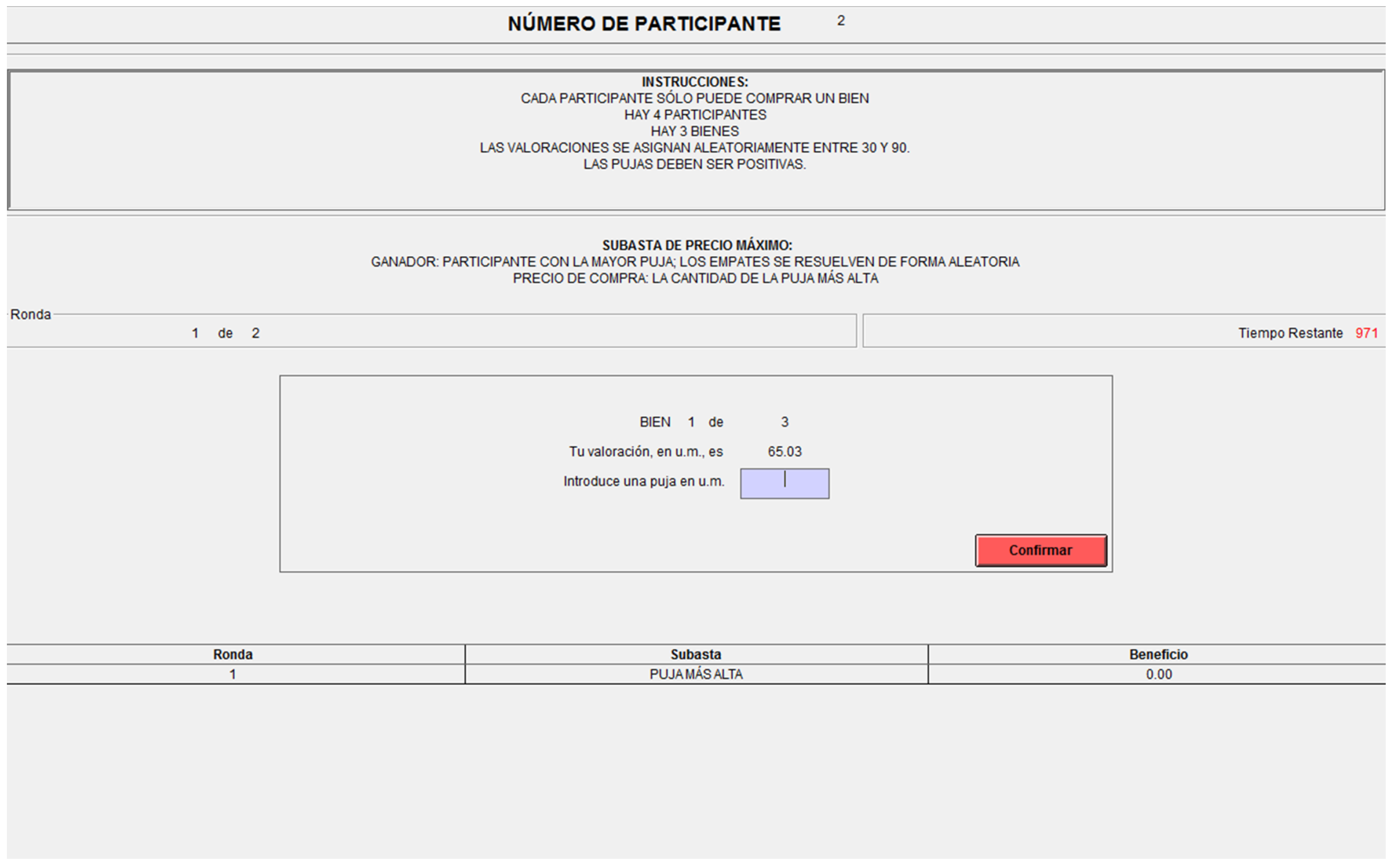
Let’s now explain the rules of each round. At the beginning of each round, the PC will assign each participant to a group with other 3 participants. For each good being auctioned, the computer will assign a random valuation between 30 and 90 tokens. The interactive screen (Figure A1) will ask the participant to enter a bid, which must be positive and less than 150 tokens, and press the confirmation button.
Figure A1.
Placing a bid.
We are facing a sealed-bid auction, since the bids are anonymous and secret, and there is a set period to time to submit the bid. That is why it is critical to remain in silence.
Before submitting the bid, it is convenient to read the information on the screen, to correctly identify the good being auctioned and to fully understand the rules:
- 4 participants in each group and 3 goods per round.
- The valuations are random between 30 and 90 tokens.
- The auction type currently under way: First Price and Second Price. The peculiarities of each of the two types will be explained later.
The rest of the available information shown on the screen is:
- The round or period.
- The remaining time to submit a bid.
- The good that it is being auctioned out of the possible 3.
- The history of the experiment, indicating the profit obtained per round.
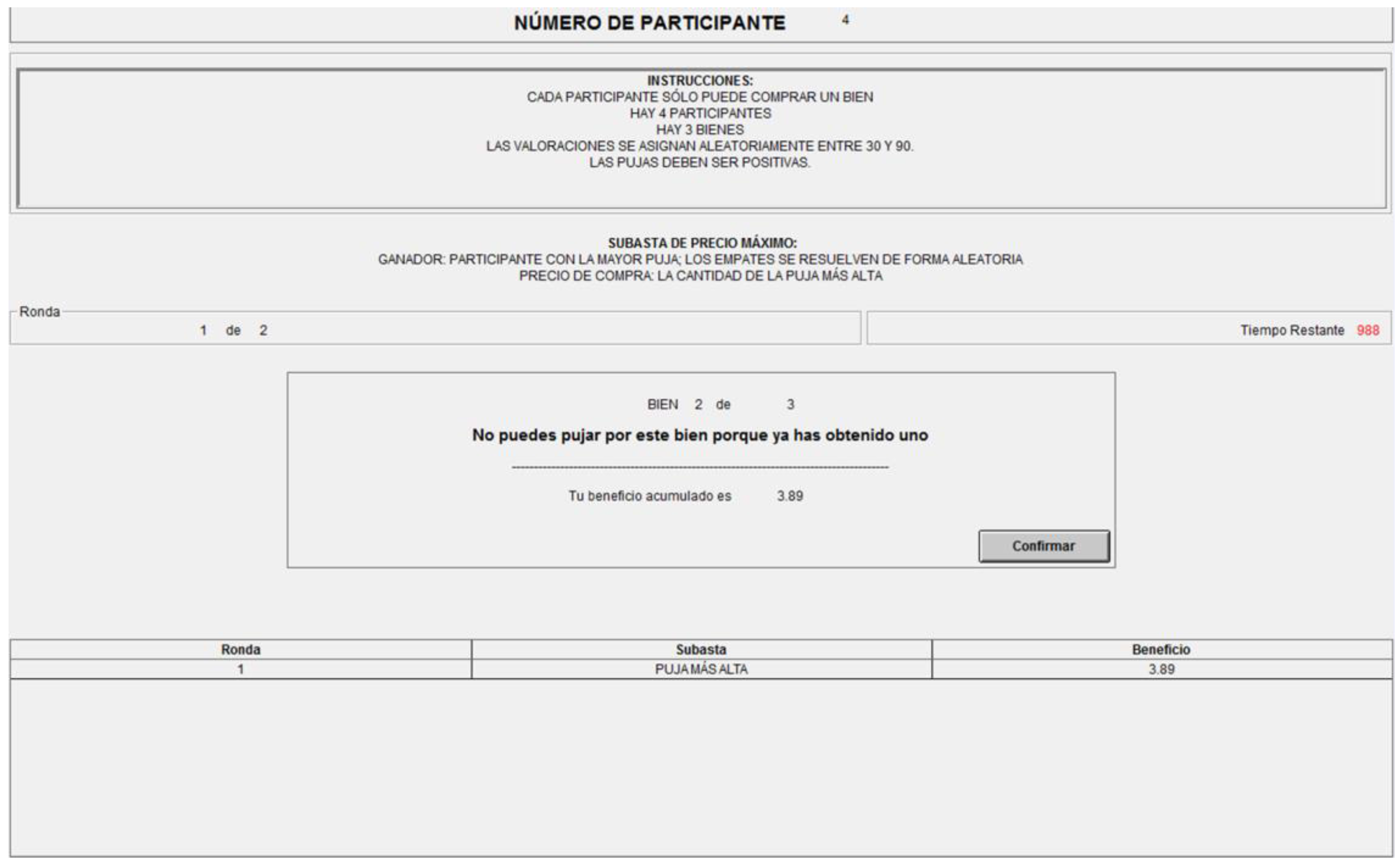
If a participant has previously obtained a good, the screen is different (Figure A2), just indicating the history, since the subject is not allowed to bid nor obtain a second good.
Figure A2.
Not allowed to bid as a previous winner.
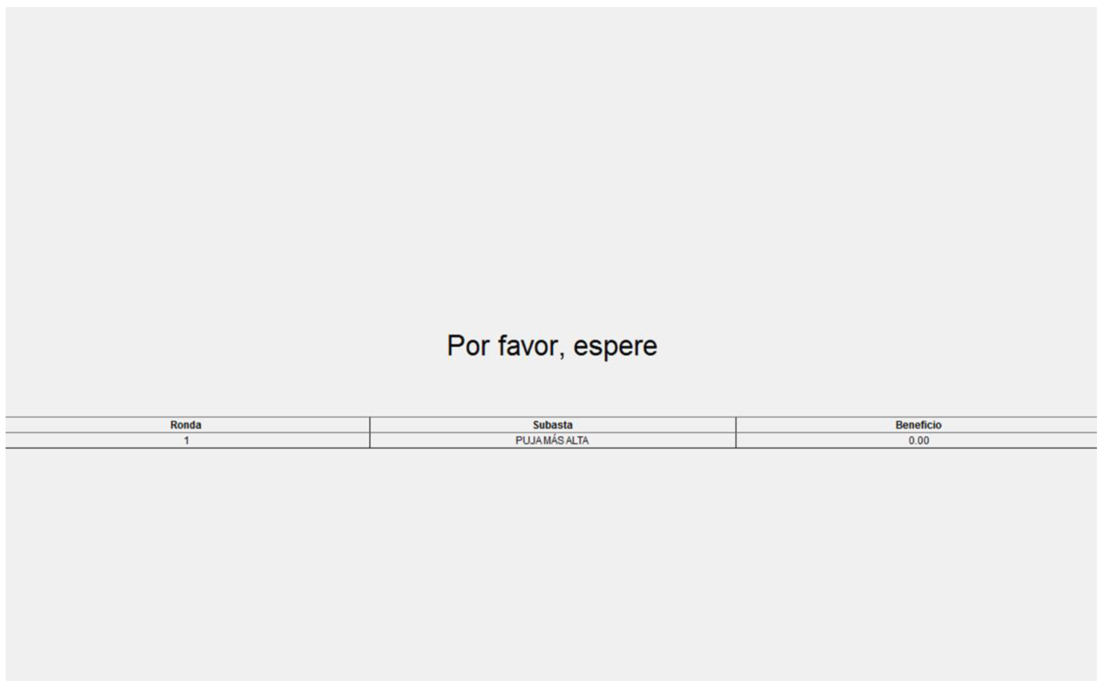
When the participants confirm their bids or their profits, a wait screen will show up (Figure A3), screen that will disappear whenever each and every participant press the corresponding confirmation button.
Figure A3.
Wait screen.
When all the bids have been submitted, the computer will assign the good to the buyer or winner, whoever placed the highest bid. The price to pay in tokens will depend on the type of auction mechanism of the current round:
- Under First Price or Maximum Price, the Price coincides with the bid placed by the winner.
- Under Second Price or Vickrey, the Price corresponds not to one’s own bid but to the second highest bid.
The profit obtained by the winner or buyer is equal then to the value minus the Price, being positive if the Price is lower than the valuation and negative if the price is above the valuation.
Following you will see simple screenshots with examples that may show up after the assignment of the good to the winner, screens that vary depending on the auction mechanism and the participant is the winner or not.
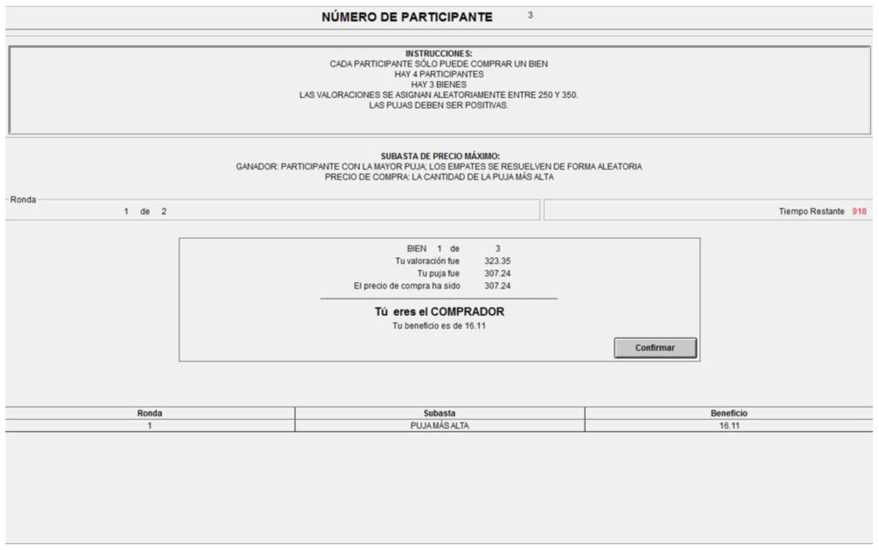
The first screenshot (Figure A4) will be seen by the winner of a First Price auction, and the profit is one’s own valuation minus one’s own bid.
Figure A4.
Winner of F.
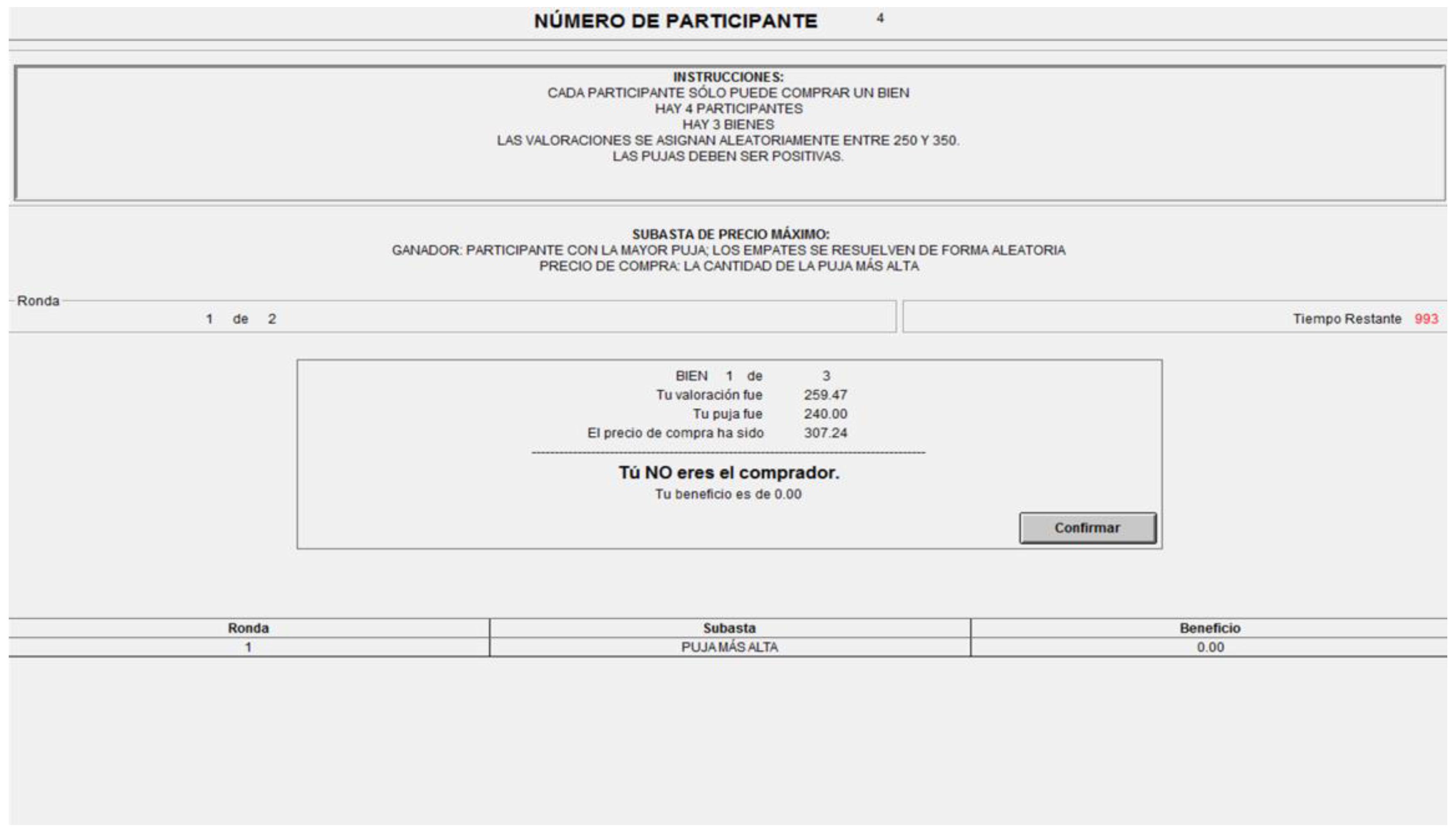
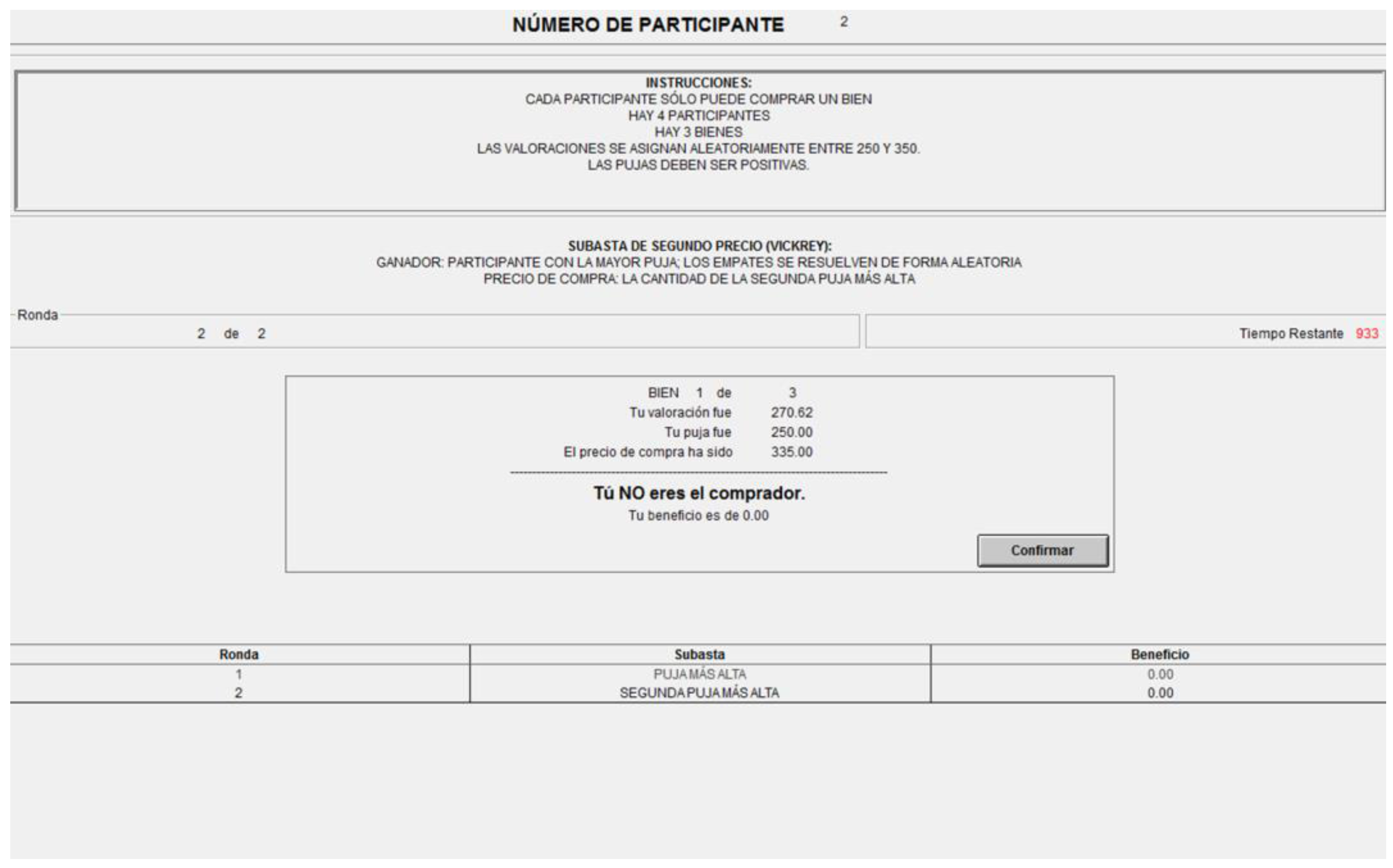
The second (Figure A5) corresponds to a non-winner in a First Price auction.
Figure A5.
Non-winner of F.

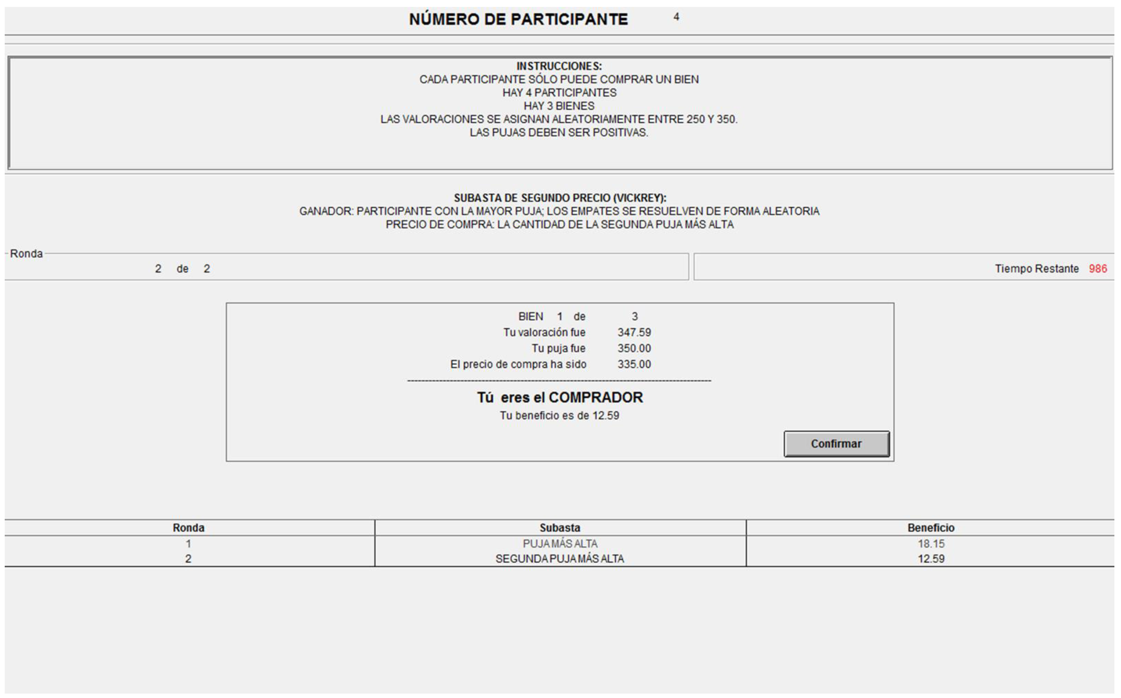
The third screen (Figure A6) corresponds to the winner of a Second Price auction, with its bid of 350 tokens and a Price to pay of 335 tokens, so the profit is, given the valuation of 347.59, of 12.59 tokens.
Figure A6.
Winner of S.
The fourth screenshot (Figure A7) corresponds to a non-winner of a Second Price auction, with a bid of 250, and a Price of 335 tokens.
Figure A7.
Non-winner of S.

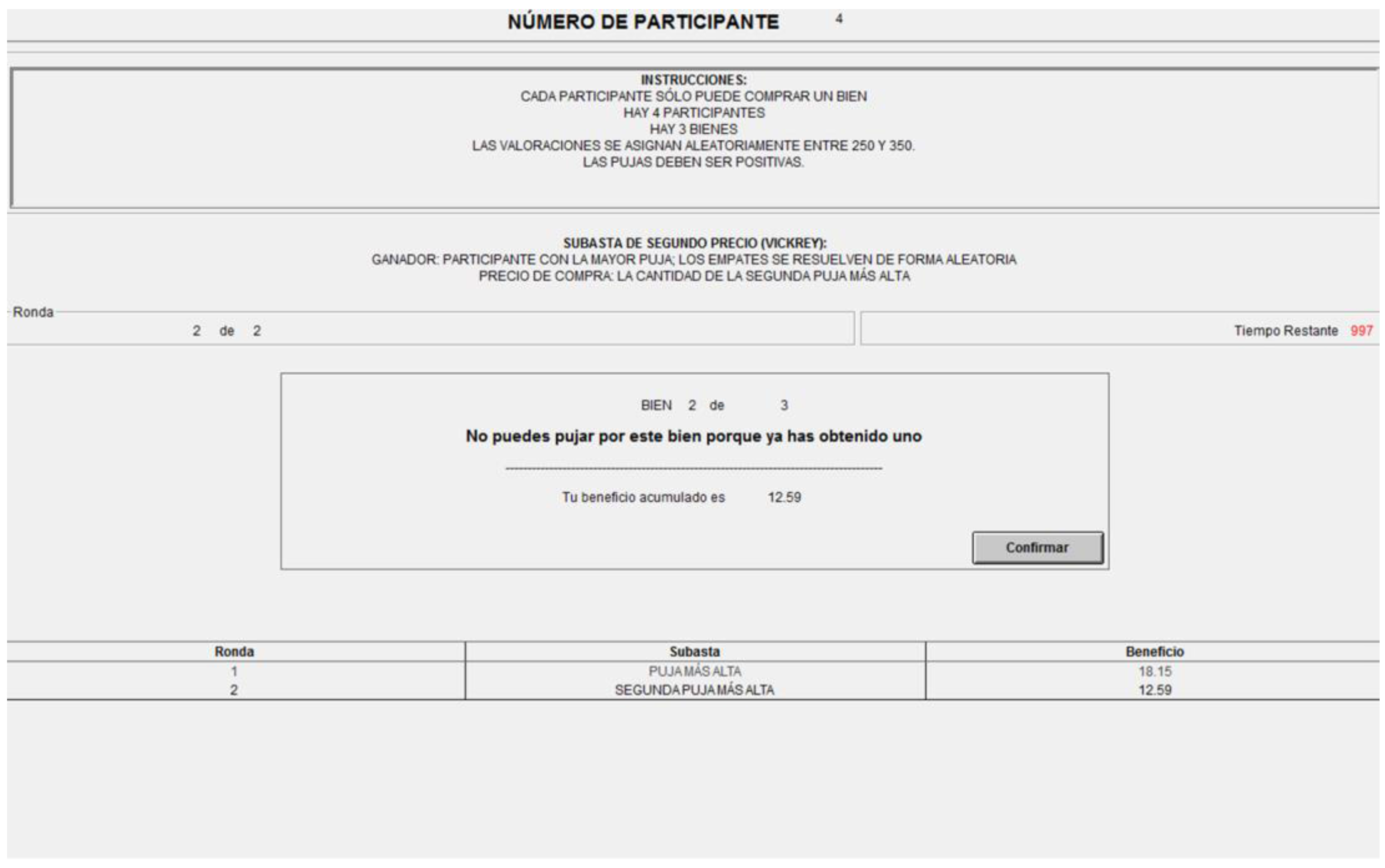
The last screen (Figure A8) shows the history of the profits for a participant that cannot bid.
Figure A8.
History of profits.

Obviously, the numbers are fictitious since they are not within the allowable range for this experiment, since the valuations will be between 30 and 90 for everyone.
As a summary, each round is composed of the following stages:
- Assignment of participants to groups
- For each group:
- Auction for Good 1 of 3: Placement of 4 bids and assignment to the winner
- Auction for Good 2 of 3: Placement of 3 bids and assignment to the winner
- Auction for Good 3 of 3: Placement of 2 bids and assignment to the winner
- Presentation of profits in tokens after each good and auction
At the end of each round, the following screen (Figure A9) will appear, asking to wait for instructions:
Figure A9.
End of round.
8 rounds will be played, the first 4 will be First Price/Second Price and the last 4 will be Second Price/First Price. A practice round will be performed first.
At the end of the experiment, after the 8 rounds, one round will be selected at random to convert the tokens obtained in that round in euros. Once the round is select, I will individually and secretly pay in euros at a conversion rate of 1 euro per 4 tokens. 2 additional euros will be payed to each individual to cover the participation.
We will now start the experiment. Please follow the instructions that I will dictate out loud.
Appendix C. Comprehension Quiz
- How many rounds of FIRST PRICE auctions are there?
- 1
- 4
- 8
- How many rounds of SECOND PRICE auctions are there?
- 1
- 4
- 8
- In each round, how many participants are there in each group?
- 1
- 3
- 4
- 8
- In each round, how many goods are auctioned in each group?
- 1
- 3
- 4
- 8
- In each round, how are the goods auctioned?
- All at once
- Sequentially
- If you win the first good in a given round, are you allowed to bid for the second good in that round?
- Yes
- No
- If you do not win the first good in a given round, are you allowed to bid for the second good in that round?
- Yes
- No
- If your valuation in a round is 234.56, your bid is 210.98, which is the highest bid, and the second highest bid is 200.00, what is your profit if the auction type is FIRST PRICE?
- 234.56–210.98
- 234.56–200.00
- 210.98–200.00
- If your valuation in a round is 234.56, your bid is 210.98, which is the highest bid, and the second highest bid is 200.00, what is your profit if the auction type is SECOND PRICE?
- 234.56–210.98
- 234.56–200.00
- 210.98–200.00
- What is your final profit in euros?
- The sum of the profits in tokens of each round divided by 4 plus 2 euros
- The average of the profits in tokens of each round divided by 4 plus 2 euros
- The profit in tokens of one round selected at random divided by 4 plus 2 euros
Appendix D. Supplemental Analysis
Appendix D1. Regression Analysis Controlling for Intra-Groups Correlations
(a) Groups defined as session and order
An alternative model consists in assuming that all observations within a session featuring a specific order are correlated. In that case, we should assume there are only 3 independent groups in the order [F,S] and 3 independent groups in the order [S,F]. The results are reported in Table A1 and Table A2.

Table A1.
Regression analysis of bids by auction type.
| Bid in FIRST | Bid in SECOND | |||
|---|---|---|---|---|
| (1) | (2) | (3) | (4) | |
| Value | 0.93 *** | 0.93 *** | 0.94 *** | 0.99 *** |
| (0.03) | (0.05) | (0.03) | (0.03) | |
| Constant (at ) | 25.77 | 24.45 | 32.20 * | 29.66 |
| (2.83) | (3.62) | (1.97) | (2.09) | |
| G2 | 3.62 *** | 2.19 | 0.61 | 4.35 |
| (0.69) | (4.51) | (0.72) | (3.88) | |
| G3 | 3.03 ** | 2.94 | 0.72 | 9.78 *** |
| (0.98) | (3.013) | (1.44) | (2.18) | |
| Value * G2 | 0.02 | −0.06 | ||
| (0.08) | (0.06) | |||
| Value * G3 | 0.001 | −0.14 *** | ||
| (0.06) | (0.04) | |||
| Order | 3.10 | 1.98 | ||
| (3.71) | (3.09) | |||
| # obs. | 720 | 720 | 720 | 720 |
| # clusters | 6 | 6 | 6 | 6 |
| Adj. R squared | 0.60 | 0.60 | 0.63 | 0.64 |
* significant at 5% level; ** significant at 1% level; *** significant at 0.1% level; std. errors in parenthesis. (No relevant null hypothesis on constant: no inference is reported).
Table A2.
Regression analysis of bids across auctions.
| (1) | (2) | (3) | |
|---|---|---|---|
| Value | 0.93 *** | 0.96 *** | 0.95 *** |
| (0.02) | (0.03) | (0.04) | |
| Constant (at ) | 26.51 | 24.54 | 24.56 |
| (2.66) | (2.90) | (3.02) | |
| G2 | 2.11 *** | 3.44 | 3.45 |
| (0.41) | (3.31) | (3.31) | |
| G3 | 1.88 *** | 6.71 *** | 6.71 *** |
| (0.33) | (1.01) | (1.03) | |
| Second | 5.05 *** | 5.09 *** | 4.99 *** |
| (1.13) | (1.15) | (1.51) | |
| Value * G2 | −0.02 | −0.02 | |
| (0.06) | (0.06) | ||
| Value * G3 | −0.08 *** | −0.08 *** | |
| (0.02) | (0.02) | ||
| Order | 2.52 | 2.52 | |
| (3.24) | (3.24) | ||
| Value * Second | 0.002 | ||
| (0.02) | |||
| # obs. | 1440 | 1440 | 1440 |
| # clusters | 6 | 6 | 6 |
| Adj. R squared | 0.62 | 0.63 | 0.63 |
* significant at 5% level; ** significant at 1% level; *** significant at 0.1% level; std. errors in parenthesis. (No relevant null hypothesis on constant: no inference is reported).
Note that the results are very similar to the results reported in Table 5 and Table 6, except for a significant interaction between Value and G3 driven by S.
(b) Groups within sessions
In each session and each round, groups of 4 are formed. In any session with 12 participants, 3 groups are formed in each round for a total of 12 groups formed over the session to play F and another 12 groups formed to play S. In any sessions of 16 participants, 16 groups are formed over the session to play F and another 16 groups formed to play S. Overall, for each auction type, the number of groups is 12 × 4 + 16 × 2 = 80. We report below the regression analysis presented in Table A3 and Table A4 taking into account within group correlations. We report below the regression analysis presented in Table A3 and Table A4 taking into account within group correlations.
Table A3.
Regression analysis of bids by auction type.
| Bid in FIRST | Bid in SECOND | |||
|---|---|---|---|---|
| (1) | (2) | (3) | (4) | |
| Value | 0.93 *** | 0.92 *** | 0.94 *** | 0.99 *** |
| (0.03) | (0.05) | (0.03) | (0.047) | |
| Constant (at ) | 25.77 | 24.44 | 32.20 * | 29.66 |
| (2.20) | (3.16) | (1.59) | (2.63) | |
| G2 | 3.62 *** | 2.19 | 0.61 | 4.35 |
| (0.93) | (4.70) | (0.96) | (3.33) | |
| G3 | 3.03 ** | 2.94 | 0.72 | 9.78 * |
| (0.99) | (4.36) | (1.30) | (3.89) | |
| Value * G2 | 0.02 | --- | −0.06 | |
| (0.08) | (0.06) | |||
| Value * G3 | 0.001 | −0.14 * | ||
| (0.07) | (0.06) | |||
| Order | 3.10 * | 1.98 | ||
| (1.40) | (1.87) | |||
| # obs. | 720 | 720 | 720 | 720 |
| # clusters | 80 | 80 | 80 | 80 |
| Adj. R squared | 0.60 | 0.60 | 0.63 | 0.64 |
* significant at 5% level; ** significant at 1% level; *** significant at 0.1% level; std. errors in parenthesis. (No relevant null hypothesis on constant: no inference is reported).
Table A4.
Regression analysis of bids across auctions.
| (1) | (2) | (3) | |
|---|---|---|---|
| Value | 0.93 *** | 0.96 *** | 0.95 *** |
| (0.02) | (0.03) | (0.04) | |
| Constant (at ) | 26.51 | 24.54 | 24.56 |
| (1.47) | (2.17) | (2.55) | |
| G2 | 2.11 ** | 3.44 | 3.45 |
| (0.67) | (2.86) | (2.86) | |
| G3 | 1.88 * | 6.71 * | 6.71 * |
| (0.81) | (2.94) | (2.95) | |
| Second | 5.05 *** | 5.09 *** | 4.99 |
| (0.95) | (0.93) | (2.68) | |
| Value * G2 | −0.02 | −0.02 | |
| (0.05) | (0.05) | ||
| Value * G3 | −0.08 | −0.08 | |
| (0.05) | (0.05) | ||
| Order | 2.52 ** | 2.52 ** | |
| (0.94) | (0.93) | ||
| Value * Second | 0.002 | ||
| (0.04) | |||
| # obs. | 1440 | 1440 | 1440 |
| # clusters | 80 | 80 | 80 |
| Adj. R squared | 0.62 | 0.63 | 0.63 |
* significant at 5% level; ** significant at 1% level; *** significant at 0.1% level; std. errors in parenthesis. (No relevant null hypothesis on constant: no inference is reported).
Again, the inferences drawn from this other specification of correlations are similar to what was obtained with the previous 2 specifications. The main difference is that Order effects become significant sometimes.
The main interest of the exercise presented in this Appendix is that the main inferences are not disturbed by assumptions the econometricians makes about what is the independent unit of study.
To further check the robustness of the results, we ran fixed effects regressions to model unobserved heterogeneity in our sample (across participants and across groups). The results (not reported here but available upon request) are virtually the same, featuring a significant interaction between Value and G3 in some specifications of the model but not in others.
Appendix D2. Overbidding
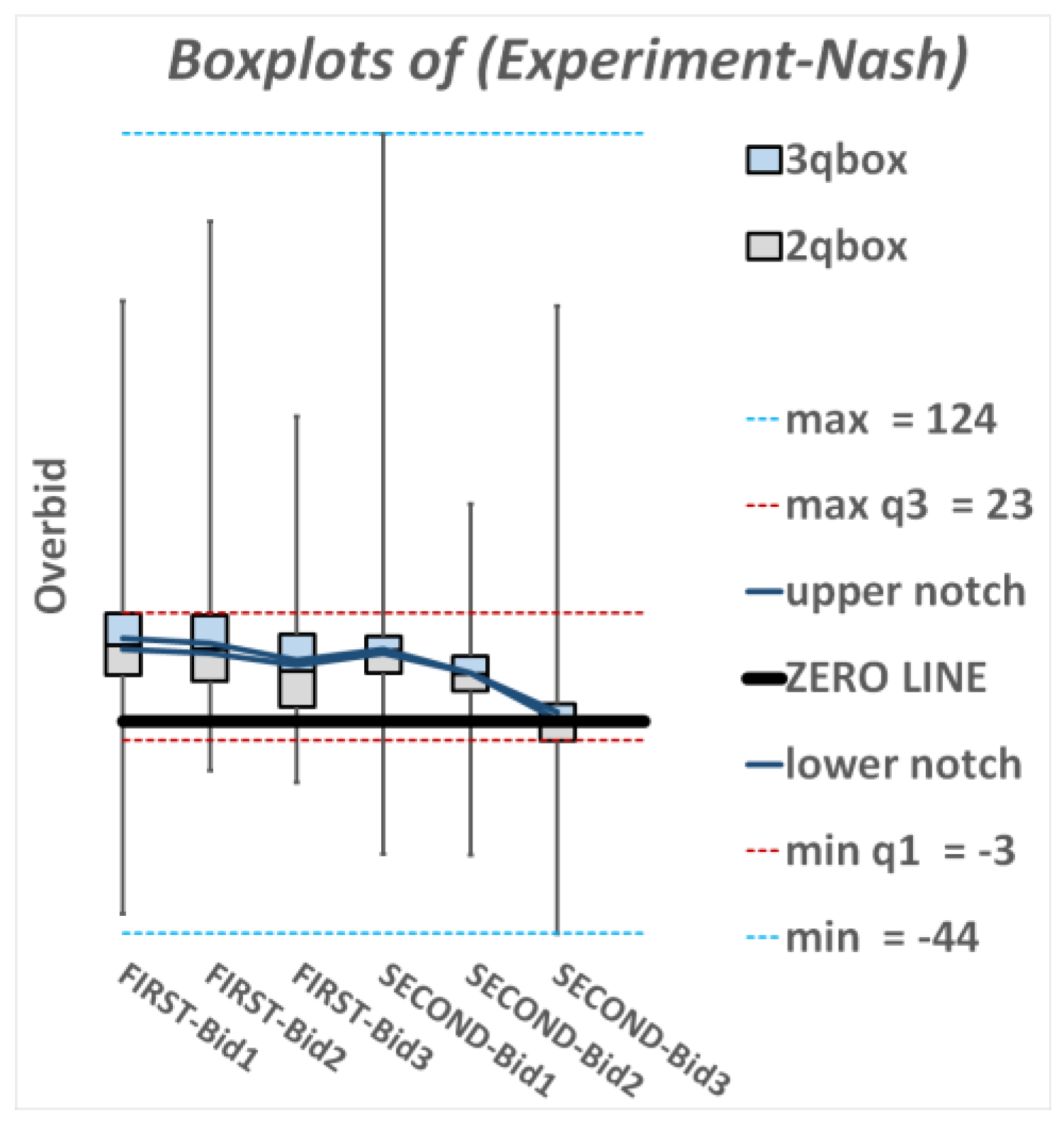
We represent for each good and mechanism the average difference between the empirical and theoretical bids (from now on called “overbid”) using boxplots. Figure A10 shows a boxplot per mechanism and good, with the box height indicating the interquartile range (q3–q1) and the line in the middle of the box illustrating the median (q2). The whiskers’ edges indicate maximums and minimums. For comparative purposes, the graph also includes the overall range (max–min) and the overall interquartile range (max q3–min q1). Finally, the notches indicate the 95% confidence intervals on the median and are connected with straight lines to ease the comparison on central tendencies across goods and types of auctions.
Figure A10.
Boxplots of average overbids.

From the boxplot, we notice an overbidding tendency that diminishes over goods. This is in line with the results in the previous subsection, where we showed that the empirical bidding strategies are similar across goods whereas the theoretical strategies are increasing across goods. Interestingly, the median bid for G3 in S is right on the equilibrium. Table A5 with the statistical comparison of medians confirms these findings: there is decreased overbidding across goods both in F (1 = 2 > 3 as shown in row 1) and in S (4 > 5 > 6 as shown in row 2). The tendency to overbid is also greater in F than in S for G2 and G3 (row 3).
Table A5.
Comparison of median bids across goods and mechanisms.
| Across Goods (FIRST) | 1 = 2 | 1 > 3 | 2 > 3 |
| Across Goods (SECOND) | 4 > 5 | 4 > 6 | 5 > 6 |
| Across Mechanisms (G1, G2, G3) | 1 = 4 | 2 > 5 | 3 > 6 |
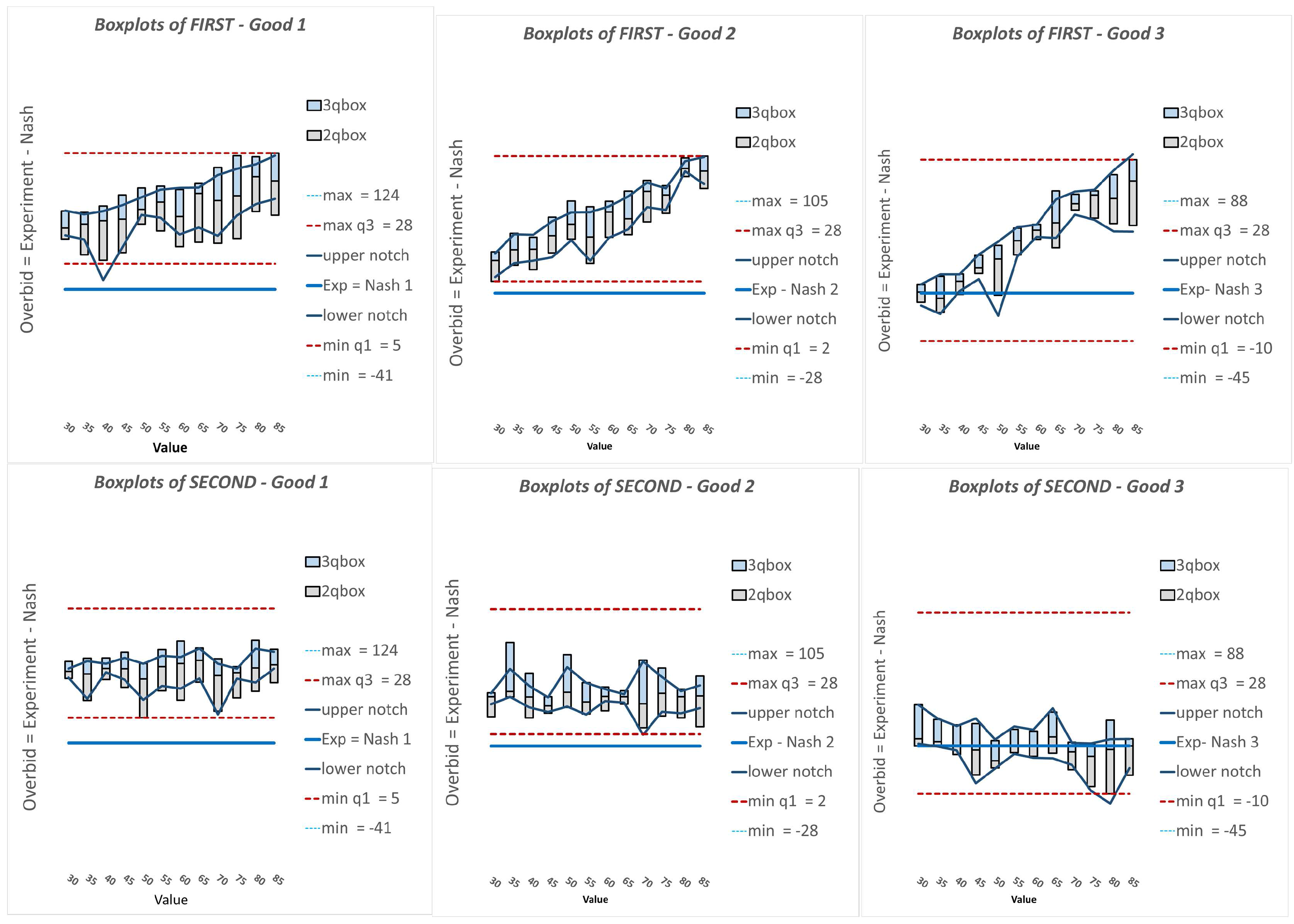
This analysis reinforces the result of consistent overbidding for all valuations, mechanisms and goods, except for G3 in S. More interestingly, within a good, overbidding increases significantly with valuation in F (reaching a median overbid of 28 units for the highest valuation bin) but it is remarkably constant in S (Figure A11). Again, the result is consistent with the findings in the section that includes the aggregate bidding functions, which emphasized that bids are excessively sensitive to valuation in F (above 0.90 when the theory predicts 0.50 to 0.75). By contrast, in S a one-unit increase in valuation translates into an almost one-unit increase in bid, just like the theory predicts. For the case of G3 in S, the median bidding is remarkably close to Nash in all valuation bins.
Figure A11.
Boxplots of overbids per good and mechanism.

Appendix D3. Payoffs
The methodology to compare theoretical and experimental payoff functions (PF) is the same as the one followed to analyze bidding functions. We are interested in finding the payoff obtained by the winner of the auction who, in theory, is also the highest valuation subject but in practice may not. The first graph of Figure A12 represents the theoretical net payoff of the winner (value minus own bid for F and value minus expected second-highest bid for S which, as we know from the theory section, are identical). The graph is therefore an affine transformation of the theoretical bidding function in F shown previously ( instead of only ), so it is again linear in . The second graph shows the empirical payoffs. In the x-axis, valuations are, once again, grouped in bins of 5. The y-axis shows the average net payoff of winners with valuations in that bin. The third graph includes a linear OLS regression to estimate the best fit of the winner’s payoff function:
It is important to notice the censored data aspect of the information reported compared to the bidding data presented previously, as we now only consider the values and bids of the highest (winning) bidder. Since there are very few observations of winning bids for values below 40 (between 0 and 4 depending on the good and mechanism) and they typically correspond to outliers who greatly overbid, we only report in the graphs the results for values above 40.
As before, we also present a table with slopes and intercepts at v = 30 of the theory and the OLS regression with their corresponding standard errors clustered at the individual level (Table A6). It also shows the results of a t-test of comparison between the two.
Figure A12.
Payoff functions.
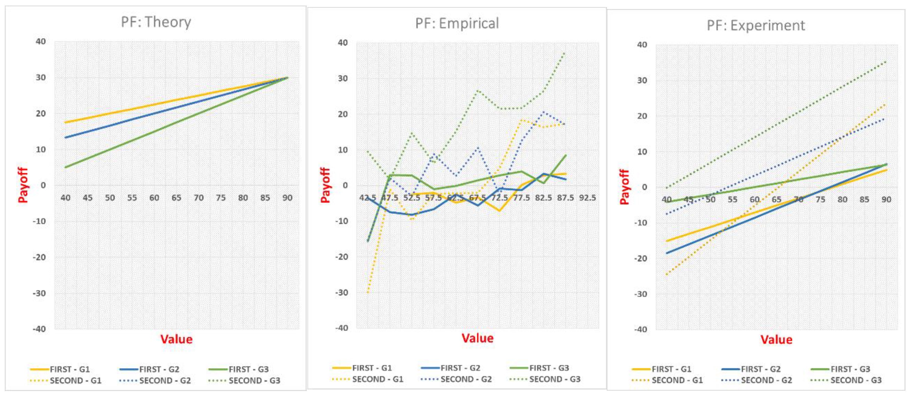
Table A6.
Comparison of payoff functions.
| FIRST | SECOND | ||||||
|---|---|---|---|---|---|---|---|
| G1 | G2 | G3 | G1 | G2 | G3 | ||
| SLOPE | Theory | 0.25 | 0.33 | 0.50 | 0.25 | 0.33 | 0.50 |
| Experiment | 0.40 | 0.50 | 0.21 † | 0.96 * | 0.54 * | 0.71 | |
| Std. Error | 0.15 | 0.19 | 0.10 | 0.15 | 0.09 | 0.12 | |
| INTERCEPT (at ) | Theory | 15.00 | 10.00 | 0.00 | 15.00 | 10.00 | 0.00 |
| Experiment | −19.12 † | −23.53 † | −6.24 | −33.97 † | −12.90 † | −7.24 | |
| Std. Error | 11.64 | 14.52 | 7.68 | 12.28 | 6.24 | 8.66 | |
* significantly higher than theory at 5% level; † significantly lower than theory at 5% level.
Theory and data are quite different. Consistent with decreased overbidding over goods, the payoff of the winner is significantly larger in G3 compared to G2 and G1 in both auctions, which is the opposite of the theoretical prediction. Bids are also substantially more responsive to values in S (significantly above theory in G1 and G2) compared to F. Finally, and again in accordance to previous results, profits are higher in S than in F for all goods, especially for high valuations.
Following a similar methodology as for the analysis of bids, we can also perform a regression of the payoff of the winner as a function of the value, with dummies for goods and mechanisms. The results are reported in Table A7.
Table A7.
Regression analysis of payoffs of winner.
| Payoff in F | Payoff in S | Payoff | |
|---|---|---|---|
| Value | 0.36 *** | 0.71 *** | 0.54 *** |
| (0.10) | (0.07) | (0.06) | |
| Constant (at ) | −17.70 | −22.38 | −27.22 |
| (8.35) | (6.14) | (5.27) | |
| G2 | −0.50 | 2.01 | 1.02 |
| (2.50) | (2.06) | (1.60) | |
| G3 | 5.50 * | 15.05 *** | 10.72 *** |
| (0.97) | (2.17) | (1.73) | |
| Second | --- | --- | 14.00 *** |
| (1.22) | |||
| # obs. | 720 | 720 | 1440 |
| # clusters | 80 | 80 | 80 |
| Adj. R squared | 0.11 | 0.39 | 0.39 |
* significant at 5% level; ** significant at 1% level; *** significant at 0.1% level; std. errors in parenthesis. (No relevant null hypothesis on constant: no inference is reported).
The regression clearly shows that bidders earn significantly higher payoffs in G3 than in G1 or G2 and in S than in F. The result is not surprising. Indeed, the similar (though, as we already discussed, not identical) bidding strategy in all 6 cases, means less overbidding hence higher profits for the winner in later auctions and in second-price auctions. Payoffs are also more reactive to value in S than in F.
Appendix D4. Payoffs Across Clusters
The last step of our analysis consists in studying the winner’s payoffs in each cluster. We follow the same methodology as we did for overbidding and present in Table A8 the average payoffs across goods and mechanisms, separately for each cluster.
Table A8.
Average payoff of winner per cluster in tokens.
| Good | EE | EL | LE | LL | Total | Theory | ||||||
|---|---|---|---|---|---|---|---|---|---|---|---|---|
| F | S | F | S | F | S | F | S | F | S | All | ||
| G1 | −13.8 | −0.7 | 4.2 | 16.8 | 0.5 | 12.4 | 1.4 | 13.5 | −0.9 | 10.7 | 4.9 | 27.0 |
| G2 | −14.1 | 9.6 | 0.5 | 18.7 | 5.2 | 9.6 | −3.6 | 7.8 | −3.7 | 10.3 | 3.3 | 25.0 |
| G3 | −11.2 | 26.3 | −9.2 | 26.3 | 4.3 | 20.2 | 3.4 | 23.3 | 1.8 | 23.8 | 12.8 | 20.0 |
| Avg. | −13.5 | 7.2 | 1.3 | 22.4 | 3.4 | 12.4 | 0.7 | 16.5 | −0.9 | 14.9 | 7.0 | 24.0 |
The results in F are stark. Early winners incur in either severe losses (EE) or small gains (EL). They seldom reach G3 but when they do, they still overbid and lose substantial money. Late winners (LE and LL) avoid losses but they still do not obtain high payoffs for two reasons: because they still (moderately) overbid and because their rivals overbid. The difference between clusters is most significant in G3 where EE and LE lose 10 tokens on average whereas EL and LL, who face early winners less frequently, win 4 tokens. Overall, for the most rational bidders, patience pays off: contrary to the theory, earnings in G3 are higher than in G1 or G2 due to the self-selection effect.
Results are slightly more mixed in S. On the one hand, the tendency of late winners (EL and LL) to overbid less than early winners (EE and LE) implies that the former obtain larger gains than the latter: 22.4 and 16.5 vs. 7.2 and 12.4. On the other hand, and contrary to F, patience pays off for all subjects: in all four clusters, the highest profits are obtained in G3 under S (and these gains are typically higher than predicted by theory). This counterintuitive result has a simple explanation. In G3 there are only two bidders, so if an EE or LE wins the good over an EL or LL, his bid is irrelevant for payoff purposes since he will pay the price set by his rival’s bid. In other words, in G3 mistakes of the form of overbidding are less costly under S than under F, and this is reflected in the gains of “early” subjects in G3.
References
- Kagel, J.H.; Levin, D. Auctions: A Survey of Experimental Research. In The Handbook of Experimental Economics; Kagel, J.H., Roth, A.E., Eds.; Princeton University Press: Princeton, NJ, USA, 2015; Volume 2, pp. 5636–5637. ISBN 978-0691139999. [Google Scholar]
- Kwasnica, T.; Sherstyul, K. Multiunit auctions. J. Econ. Surv. 2013, 277, 461–490. [Google Scholar] [CrossRef]
- Ashenfelter, O. How auctions work for wine and art. J. Econ. Perspect. 1989, 33, 23–36. [Google Scholar] [CrossRef]
- Ashenfelter, O.; Genesove, D. Testing for price anomalies in real-estate auctions. Am. Econ. Rev. 1992, 822, 501–505. [Google Scholar]
- Van den Berg, G.J.; van Ours, J.C.; Pradhan, M.P. The declining price anomaly in Dutch rose auctions. Am. Econ. Rev. 2001, 91, 1055–1062. [Google Scholar] [CrossRef]
- Weber, R.J. Multiple-object auctions. In Auctions, Bidding, and Contracting; Engelbrecht-Wiggans, R., Shubik, M., Stark, R., Eds.; UP: New York, NY, USA, 1983; pp. 165–191. [Google Scholar]
- McAfee, R.P.; Vincent, D. The declining price anomaly. J. Econ. Theory 1993, 60, 191–212. [Google Scholar] [CrossRef]
- Keser, C.; Olson, M. Experimental examination of the declining-price anomaly. In Economics of the Art: Selected Essays; Ginsburgh, V.A., Menger, P.M., Eds.; Elsevier: Amsterdam, The Netherlands, 1996; pp. 151–176. ISBN 978-0444824028. [Google Scholar]
- Salmon, T.C.; Wilson, B.J. Second chance offers versus sequential auctions: Theory and behavior. Econ. Theory 2008, 34, 47–67. [Google Scholar] [CrossRef]
- Neugebauer, T.; Pezanis-Christou, P. Bidding behavior at sequential first-price auctions with(out) supply uncertainty: A laboratory analysis. J. Econ. Behav. Organ. 2007, 63, 55–72. [Google Scholar] [CrossRef]
- Brosig, J.; Reiss, P.J. Entry decisions and bidding behavior in sequential first-price procurement auctions: An experimental study. Game Econ. Behav. 2007, 58, 50–74. [Google Scholar] [CrossRef]
- Dixit, A.K.; Pindyck, R.S. Investment under Uncertainty; Princeton University Press: Princeton, NJ, USA, 1994; ISBN 978-0691034102. [Google Scholar]
- Leufkens, K.; Peeters, R. Synergies are a reason to prefer first-price auctions. Econ. Lett. 2007, 97, 64–69. [Google Scholar] [CrossRef]
- Leufkens, K.; Peeters, R.; Vorsatz, M. An experimental comparison of sequential first- and -price auctions with synergies. BE J. Theor. Econ. 2012, 12, 2. [Google Scholar] [CrossRef]
- Kagel, J.H. Auctions: A survey of experimental research. In The Handbook of Experimental Economics; Kagel, J.H., Roth, A.E., Eds.; Princeton University Press: Princeton, NJ, USA, 1995; Volume 2, ISBN 0-691-04290-X. [Google Scholar]
- Casari, M.; Ham, J.C.; Kagel, J.H. Selection bias, demographic effects, and ability effects in common value auction experiments. Am. Econ. Rev. 2007, 97, 1278–1304. [Google Scholar] [CrossRef]
- Fischbacher, U. z-Tree: Zurich Toolbox for Ready-made Economic Experiments. Exp. Econ. 2007, 10, 171–178. [Google Scholar] [CrossRef]
- Cox, J.C.; Roberson, B.; Smith, V.L. Theory and behavior of single object auctions. In Research in Experimental Economics; Smith, V.L., Ed.; JAI Press Inc.: Stamford, CT, USA, 1982; Volume 2, pp. 1–43. ISBN 0-89232-263-2. [Google Scholar]
- Isaac, R.M.; Walker, J.M. Information and conspiracy in sealed bid auctions. J. Econ. Behav. Organ. 1985, 6, 139–159. [Google Scholar] [CrossRef]
- Ockenfels, A.; Selten, R. Impulse balance equilibrium and feedback in first price auctions. Game Econ. Behav. 2005, 51, 155–170. [Google Scholar] [CrossRef]
- Neugebauer, T.; Perote, J. Bidding as if risk neutral in experimental first price auctions without information feedback. Exp. Econ. 2007, 11, 190–202. [Google Scholar] [CrossRef]
- Dorsey, R.; Razzolini, L. Explaining overbidding in first price auctions using controlled lotteries. Exp. Econ. 2003, 6, 123–140. [Google Scholar] [CrossRef]
- Neugebauer, T.; Selten, R. Individual behavior of first-price auctions: The importance of information feedback in computerized experimental markets. Game Econ. Behav. 2006, 54, 183–204. [Google Scholar] [CrossRef]
- Füllbrunn, S.; Neugebauer, T. Varying the number of bidders in the first-price sealed-bid auction: Experimental evidence for the one-shot game. Theor. Decis. 2013, 75, 421–447. [Google Scholar] [CrossRef] [Green Version]
- Kagel, J.H.; Levin, D. Behavior in multi-unit demand auctions: Experiments with uniform price and dynamic Vickrey auctions. Econometrica 2001, 69, 413–454. [Google Scholar] [CrossRef]
- Elbittar, A. Impact of valuation ranking information on bidding in first-price auctions: A laboratory study. J. Econ. Behav. Organ. 2009, 69, 75–85. [Google Scholar] [CrossRef]
- Kagel, J.H.; Levin, D. Independent private value auctions-bidder behavior in 1st-price, 2nd-price and 3rd-price auctions with varying numbers of bidders. Econ. J. 1993, 103, 868–879. [Google Scholar] [CrossRef]
- Goeree, J.K.; Holt, C.A.; Palfrey, T.R. Quantal response equilibrium and overbidding in private-value auctions. J. Econ. Theory 2002, 104, 247–272. [Google Scholar] [CrossRef]
- Güth, W.; Ivanova-Stenzel, R.; Wolfstetter, E. Bidding behavior in asymmetric auctions: An experimental study. Eur. Econ. Rev. 2005, 49, 1–27. [Google Scholar] [CrossRef]
- Filiz-Ozbay, E.; Ozbay, E.Y. Auctions with anticipated regret: Theory and experiment. Am. Econ. Rev. 2007, 97, 1407–1418. [Google Scholar] [CrossRef]
| 1 | This selection effect is related to but different from that in [16], where subjects have an initial endowment and those with financially poor decisions go bankrupt and are forced to leave the auction. Our selection is more directed. In each round, two bidders out of four win goods 1 and 2. They exit and cannot bid for good 3. |
| 2 | We thank an anonymous referee for highlighting this important point. |
| 3 | Indeed, since all bidders at period t decrease their bid by VFt+1 compared to a static auction and there is no reserve price, the winner’s payoff is increased by that amount and the losers’ payoff is also increased by that amount (the value of going to the next stage). |
| 4 | So, within each round, all three goods were allocated using the same mechanism (first- or second-price auction) but with different number of bidders (4, 3 or 2). |
| 5 | If the selected round implied a negative payoff for a subject, we did not ask that participant to pay money back. Limited liability may have had an impact on the behavior of some subjects, although we conjecture that a small one. |
| 6 | The two reasons for the low payment were excessively low conversion rate and significant overbidding. |
| 7 | Surprisingly, a large fraction of the most recent articles in this literature does not discuss efficiency. |
| 8 | Formally, if the highest valuation is x and the winner has valuation y, the efficiency is (y − 30)/(x − 30). This measure corrects for the fact that not all inefficiencies are equally severe. We thank an anonymous referee for suggesting it. |
| 9 | Design choices vary sharply regarding whether to allow bids above value. In many experiments those bids are prevented [19,20,21], discouraged by design [22,23,24] or presented as “wrong” during instructions [10,25,26]. In the rare cases in which bids above value are allowed and not framed any way, some are observed although fewer than in our paper [27,28,29]. |
| 10 | The excessive similarity between bids in F and S relative to the theoretical predictions will be a recurrent result of our analysis. It is particularly noticeable given our within-subject design, which typically exacerbates differences in behavior vía an experimenter demand effect. |
| 11 | We provide a detailed descriptive analysis of overbidding behavior in Appendix D2. |
| 12 | We tried also to cluster subjects in 2 or 3 groups, but the results were not as sharp and they did not lend to a clean test of our hypotheses. |
| 13 | This is not very different from what would occur if all subjects played the equilibrium strategies. Indeed, given our (endogenous) definition of clusters, we would statistically obtain 47% of LL, 10% of EE, 21% of EL and 21% of LE. |
| 14 | Indeed, if each subject sometimes overbids and sometimes not, whenever a subject overbids he will be more likely to win G1 or G2 and therefore be classified as an E. However, if that were the case, there would be no reason why that subject would also overbid consistently and significantly more than the other subjects also in G3. |
| 15 | What follows are the instructions in English. The Spanish version, the one that was used, is available upon request. The screenshots have not been translated. |
Figure 1.
Bidding functions.
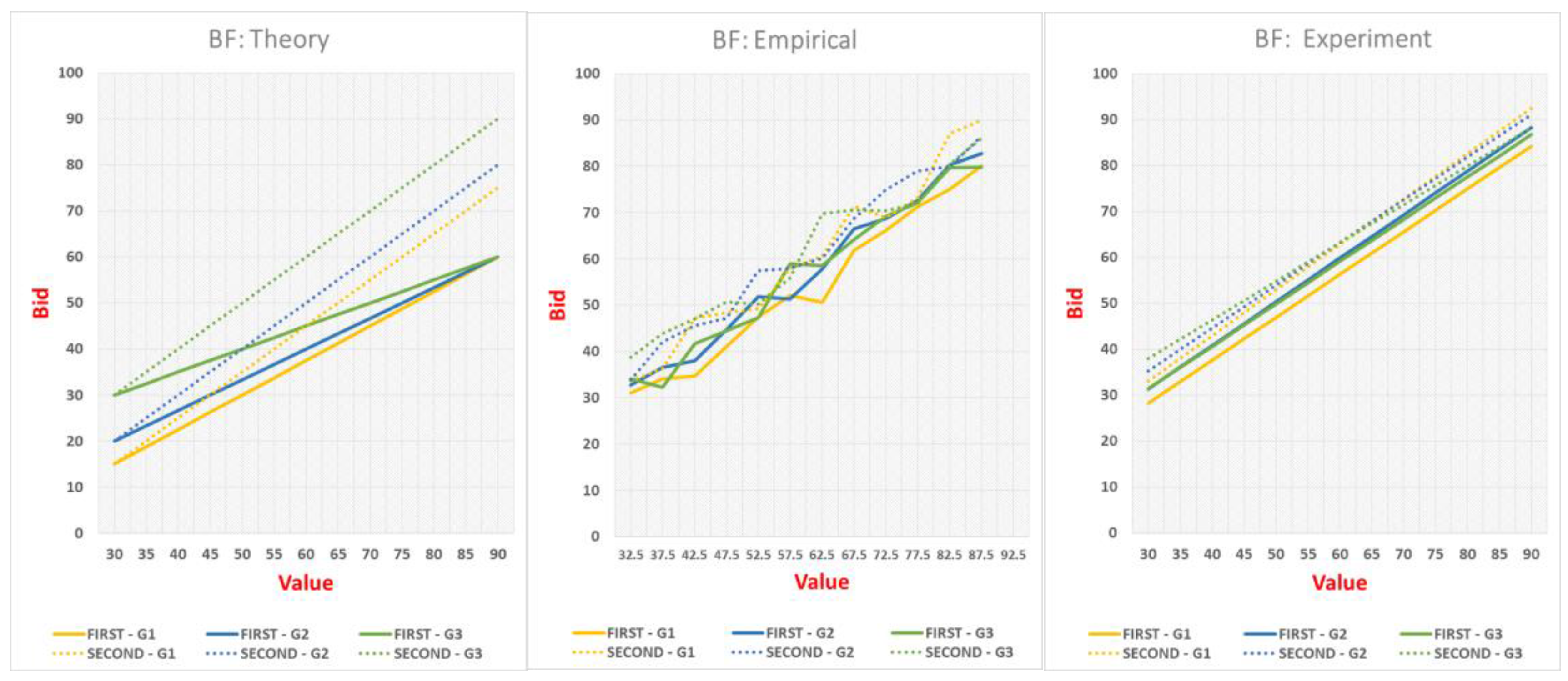
Figure 2.
Clusters.

Table 1.
Average efficiency (percentage).
| Good | Allocation Efficiency | Surplus Efficiency | ||
|---|---|---|---|---|
| F | S | F | S | |
| G1 | 62.5 | 71.3 | 93.3 | 92.3 |
| G2 | 68.8 | 62.5 | 90.9 | 92.5 |
| G3 | 87.5 | 93.8 | 95.9 | 97.9 |
| Overall | 72.9 | 75.8 | 93.4 | 94.2 |
Table 2.
Average payoff of winner in tokens.
| Good | F | S | |
|---|---|---|---|
| G1 | Theory | 27.0 | 27.0 |
| Experiment | −0.9 | 10.7 | |
| Std. error * | 2.3 | 2.1 | |
| G2 | Theory | 25.0 | 25.0 |
| Experiment | −3.7 | 10.3 | |
| Std. error * | 2.3 | 1.7 | |
| G3 | Theory | 20.0 | 20.0 |
| Experiment | 1.8 | 23.8 | |
| Std. error * | 1.4 | 1.9 | |
Table 3.
Bids above valuation in F.
| Indicators | F | ||
|---|---|---|---|
| G1 | G2 | G3 | |
| Mean bid over valuation | 11.98 | 15.50 | 10.87 |
| Median bid over valuation | 8.75 | 9.74 | 5.12 |
| Fraction of observations | 0.19 | 0.20 | 0.17 |
Table 4.
Comparison of bidding functions.
| F | S | ||||||
|---|---|---|---|---|---|---|---|
| G1 | G2 | G3 | G1 | G2 | G3 | ||
| SLOPE | Theory | 0.75 | 0.67 | 0.50 | 1.00 | 1.00 | 1.00 |
| Experiment | 0.93 * | 0.95 * | 0.92 * | 1.00 | 0.93 | 0.84 *† | |
| Std. Error | 0.04 | 0.06 | 0.05 | 0.05 | 0.04 | 0.05 | |
| INTERCEPT (at ) | Theory | 15.00 | 20.00 | 30.00 | 15.00 | 20.00 | 30.00 |
| Experiment | 25.95 * | 28.97 * | 29.11 | 30.60 * | 32.96 * | 35.91 | |
| Std. Error | 3.02 | 3.94 | 2.85 | 2.68 | 2.68 | 3.39 | |
* significantly higher than theory at 5% level; † significantly lower than theory at 5% level.
Table 5.
Regression analysis of bids by auction type.
| Variables | Bid in F | Bid in S | ||
|---|---|---|---|---|
| (1) | (2) | (3) | (4) | |
| Value | 0.93 *** | 0.92 *** | 0.93 *** | 0.99 *** |
| (0.03) | (0.05) | (0.03) | (0.045) | |
| Constant (at ) | 25.77 | 24.44 | 32.20 * | 29.66 |
| (2.29) | (3.32) | (1.72) | (2.83) | |
| G2 | 3.62 *** | 2.19 | 0.61 | 4.35 |
| (1.01) | (4.71) | (0.98) | (3.28) | |
| G3 | 3.03 ** | 2.93 | 0.72 | 9.78 * |
| (0.95) | (3.90) | (1.17) | (4.80) | |
| Value * G2 | --- | 0.02 | --- | −0.06 |
| --- | (0.08) | (0.05) | ||
| Value * G3 | --- | 0.001 | −0.14 | |
| --- | (0.06) | (0.08) | ||
| Order | --- | 3.10 | 1.98 | |
| (1.88) | (1.87) | |||
| # obs. | 720 | 720 | 720 | 720 |
| # clusters | 80 | 80 | 80 | 80 |
| Adj. R squared | 0.60 | 0.60 | 0.63 | 0.64 |
* significant at 5% level; ** significant at 1% level; *** significant at 0.1% level; std. errors in parenthesis. (No relevant null hypothesis on constant: no inference is reported).
Table 6.
Regression analysis of bids across auctions.
| (1) | (2) | (3) | |
|---|---|---|---|
| Value | 0.93 *** | 0.96 *** | 0.95 *** |
| (0.02) | (0.03) | (0.04) | |
| Constant (at ) | 26.51 | 24.54 | 24.56 |
| (1.71) | (2.53) | (3.03) | |
| G2 | 2.11 ** | 3.44 | 3.45 |
| (0.75) | (3.28) | (3.28) | |
| G3 | 1.88 * | 6.71 * | 6.71 * |
| (0.82) | (3.26) | (3.24) | |
| Second | 5.05 *** | 5.09 *** | 4.99 * |
| (1.18) | (1.17) | (2.50) | |
| Value * G2 | −0.02 | −0.02 | |
| (0.06) | (0.06) | ||
| Value * G3 | −0.08 | −0.08 | |
| (0.05) | (0.05) | ||
| Order | 2.52 | 2.52 | |
| (1.46) | (1.46) | ||
| Value * Second | 0.002 | ||
| (0.04) | |||
| # obs. | 1440 | 1440 | 1440 |
| # clusters | 80 | 80 | 80 |
| Adj. R squared | 0.62 | 0.63 | 0.63 |
* significant at 5% level; ** at 1% level; *** at 0.1% level; std. errors in parenthesis. (No relevant null hypothesis on constant: no inference is reported).
Table 7.
Regression analysis of overbids (empirical–equilibrium bid).
| Overbid in F | Overbid in S | Overbid | ||||
|---|---|---|---|---|---|---|
| (1) | (2) | (3) | (4) | (5) | (6) | |
| Value | 0.26 *** | 0.17 *** | −0.06 *** | −0.01 | 0.08 *** | 0.08 *** |
| (0.03) | (0.05) | (0.03) | (0.05) | (0.02) | (0.03) | |
| Constant (at ) | 8.33 | 9.44 | 17.20 *** | 14.67 *** | 25.77 *** | 14.94 *** |
| (2.29) | (3.32) | (1.72) | (2.83) | (1.85) | (2.61) | |
| G2 | 1.19 | −5.30 | −4.39 *** | −0.64 | −1.84 * | −2.83 |
| (1.02) | (4.71) | (0.98) | (3.28) | (0.76) | (3.36) | |
| G3 | −4.39 *** | −19.56 *** | −14.28 *** | −5.22 | −9.62 *** | −10.11 ** |
| (0.97) | (3.90) | (1.17) | (4.80) | (0.84) | (3.34) | |
| Second | --- | --- | --- | --- | −5.09 *** | −5.10 *** |
| (1.22) | (1.21) | |||||
| Value * G2 | 0.10 | −0.06 | 0.02 | |||
| (0.07) | (0.05) | (0.06) | ||||
| Value * G3 | 0.25 *** | −0.14 | 0.01 | |||
| (0.06) | (0.08) | (0.05) | ||||
| Order | 3.09 | 1.98 | 2.28 | |||
| (1.88) | (1.87) | (1.46) | ||||
| # obs. | 720 | 720 | 720 | 720 | 1440 | 1440 |
| # clusters | 80 | 80 | 80 | 80 | 80 | 80 |
| Adj. R squared | 0.12 | 0.14 | 0.16 | 0.17 | 0.11 | 0.11 |
* significant at 5% level; ** at 1% level; *** at 0.1% level; std. errors in parenthesis. (Null hypothesis on constant term: constant is equal to 0).
Table 8.
Overbid per cluster.
| Good | Overbid (Empirical–Nash) | |||||||
|---|---|---|---|---|---|---|---|---|
| EE | EL | LE | LL | |||||
| F | S | F | S | F | S | F | S | |
| G1 | 29.8 | 26.6 | 15.7 | 6.9 | 13.2 | 19.0 | 14.6 | 14.1 |
| G2 | 31.9 | 15.7 | 20.7 | 5.5 | 10.9 | 14.6 | 16.0 | 10.9 |
| G3 | 24.4 | 14.8 | 18.9 | −3.8 | 9.7 | 5.4 | 11.0 | 1.2 |
| Avg. | 30.0 | 21.7 | 17.6 | 3.5 | 11.5 | 15.9 | 14.2 | 9.7 |
Table 9.
Efficiency analysis.
| Winner Theory | Winner in Experiment | |||||||
|---|---|---|---|---|---|---|---|---|
| F | Same | Other | %Eff | S | Same | Other | %Eff | |
| LL + LE | G1 | 27 | 29 | 48% | G1 | 35 | 19 | 65% |
| EE + EL | 23 | 1 | 96% | 22 | 4 | 85% | ||
| LL + LE | G2 | 31 | 21 | 60% | G2 | 23 | 27 | 46% |
| EE + EL | 24 | 4 | 86% | 27 | 3 | 90% | ||
| LL + LE | G3 | 61 | 8 | 88% | G3 | 63 | 4 | 94% |
| EE + EL | 9 | 2 | 82% | 12 | 1 | 92% | ||
© 2018 by the authors. Licensee MDPI, Basel, Switzerland. This article is an open access article distributed under the terms and conditions of the Creative Commons Attribution (CC BY) license (http://creativecommons.org/licenses/by/4.0/).
Share and Cite
MDPI and ACS Style
Otamendi, F.J.; Brocas, I.; Carrillo, J.D. Sequential Auctions with Capacity Constraints: An Experimental Investigation. Games 2018, 9, 15. https://doi.org/10.3390/g9010015
AMA Style
Otamendi FJ, Brocas I, Carrillo JD. Sequential Auctions with Capacity Constraints: An Experimental Investigation. Games. 2018; 9(1):15. https://doi.org/10.3390/g9010015
Chicago/Turabian StyleOtamendi, F. Javier, Isabelle Brocas, and Juan D. Carrillo. 2018. "Sequential Auctions with Capacity Constraints: An Experimental Investigation" Games 9, no. 1: 15. https://doi.org/10.3390/g9010015
Note that from the first issue of 2016, this journal uses article numbers instead of page numbers. See further details here.