Achieving Perfect Coordination amongst Agents in the Co-Action Minority Game

1
Centre for Complexity Science and Department of Mathematics, Imperial College London, South Kensington Campus, London SW7 2AZ, UK
2
Department of Physics, Indian Institute for Science Education and Research, Pune 411008, India
*
Author to whom correspondence should be addressed.
Games 2018, 9(2), 27; https://doi.org/10.3390/g9020027
Submission received: 10 April 2018
/
Revised: 11 May 2018
/
Accepted: 15 May 2018
/
Published: 17 May 2018
Abstract
:We discuss the strategy that rational agents can use to maximize their expected long-term payoff in the co-action minority game. We argue that the agents will try to get into a cyclic state, where each of the agents wins exactly N times in any continuous stretch of days. We propose and analyse a strategy for reaching such a cyclic state quickly, when any direct communication between agents is not allowed, and only the publicly available common information is the record of total number of people choosing the first restaurant in the past. We determine exactly the average time required to reach the periodic state for this strategy. We show that it varies as , for large N, where the amplitude of the leading term in the log-periodic oscillations is found be .
1. Introduction
Since its introduction by Challet and Zhang in 1997, the Minority Game (MG) has become a prototypical model for the study of behavior of a system of interacting agents [1]. In the original model, the key element is the so-called “bounded rationality” of the agents: the agents are adaptive, and have limited information about the behavior of other agents. They use simple rules to decide their next move, based on the past outcomes. It is found that, for a range of parameter values, the system of agents evolves into a state, where the global efficiency is larger than possible if they simply made a random choice independent of history of the game. This is one of the simplest models of learning and adaptation by agents, that shows the complex emergent phenomena of self-organization, and coevolution in a system of many interacting agents, and has attracted much interest. The model can be solved exactly in the limit of large number of agents and large times, although this requires rather sophisticated mathematical techniques, e.g., functional integrals, and the replica method. There are nice reviews of the existing work on MG [2,3], and monographs [4,5].
However, to understand the effect of bounded rationality of the agents, it is imperative to compare this with the case where the rules of the game are same as before, but agents are rational. This led Sasidevan and Dhar to introduce a variation of the standard MG, called the Co-action Minority game (CAMG) in which the allowed moves, the stipulation about no direct communication between agents, and the payoffs for different outcomes are kept unchanged, but the agents are assumed to be fully rational, and their choice of possible strategies is not constrained in any way [6]. Studying the difference of its steady state from that of the standard Challet–Zhang Minority Game (CZMG) underscores the role of bounded rationality in the latter.
In the CAMG, the agents can use mixed strategies, and try to optimize their payoff not for the next day, but a weighted sum of their future payoffs, with higher weights for more immediate gains. It was found that the optimal strategy depends on the time horizon of agents, and overall efficiency of the system increases if the agents have a larger time horizon.
In this context, a natural question arises: what would rational agents do if they aim to maximize the expectation value of their long-term gain. In this paper, we show that rational agents can actually achieve the maximum possible payoff, by getting into a cyclic state, and discuss how they can arrive at the coordination needed for such a state. In contrast, in CZMG, where agents have only bounded rationality, the expected payoff per agent is lesser than than this by an amount of order , same as if they chose restaurants randomly, but with a smaller coefficient a. We show that the average time to reach the desired cyclic state satisfies a functional equation. We solve this equation exactly and show that the time required to reach the stationary state varies linearly with N.
We note that agents can only use the limited information publicly available to achieve this coordination. The problem becomes a coordination game [7], in the setting of an MG. In [6], it was assumed that agents decide their action based only on the previous day’s result. Here, we drop this assumption, and assume that agents have access to entire history of attendance record, and can also remember the entire history of their own earlier actions.
A problem equivalent to the one studied in this paper is this: we have agents playing a minority game, where N is a positive integer. What is the strategy the agents can use to work together to assign a unique identification number (ID) from 1 to to each agent, such that each agent knows her own ID, in least time, using only the public information of attendances in the past? Even more generally, we can think of agents that cannot communicate directly with each other, and each agent can only communicate with some central authority. The authority can send messages to agents, only in the broadcast mode, where the same message is sent to all the agents.
Even with this constraint, it is clearly possible for the agents to get unique IDs. For example, a simple strategy would be that each agent first generates a random string of some length m, and sends it to the central authority. We choose m to be large enough that the probability of two different agents generating the same string is small ( say, ). Then, the central authority arranges these bits in some ordered list (of total length bits), and broadcasts the list. Then, the agent can infer his ID from the the position of her unique string in the list. However, this scheme is clearly not optimal. What is the least number of bits that have to be broadcast to assign unique IDs to all agents, so that each agent knows her own ID? In our problem, the agents need to coordinate using only the information of the past attendance record, and their own past actions.
We describe a particular strategy to achieve this coordination. This strategy is quite efficient, in that the coordination is achieved in a time that increases only linearly with the number of agents, but we have no proof that it is the best possible. Interestingly, we find that the mean time to reach the cyclic shows log-periodic oscillations. In addition, the amplitude of the oscillations is very small (of order ). Such a small value, obtained without any fine-tuning, seems quite unexpected. The mathematical mechanism involved may be of interest in the more general context of understanding how many natural systems select some very small parameter-values (e.g., the inverse correlation length in self-organized critical systems, or the cosmological constant [8]). It is also of interest in the analysis of algorithms, where these kinds of oscillations were first encountered, and studied [9,10,11].
This paper is organized as follows. In Section 2, we define the model precisely. In Section 3, we discuss the complication due to possibility of coalition formation in the game, but argue that rational agents who, by definition, optimize their personal long-time average payoff, will aim to reach a periodic state. In Section 4, we describe a coordination strategy that will reach the cyclic state, using only the publicly available attendance information. In Section 5, we study the average time required to reach the periodic state, as a function of the number of agents. We show that the generating function for the average times satisfies a functional equation in one variable. We solve this equation exactly, and find that the expected time, when the number of agents is , asymptotically increases as for large N, and shows log-periodic oscillations, but of a very small amplitude of order . In the final Section 6, we summarize our results, and mention another model of resource allocation, called the Kolkata Paise Restaurant problem, where the optimal state is also periodic. We also discuss the relation of this study to other problems showing log-periodic oscillations.
2. Definition of the Model
We consider a set of agents, who choose between two options (say choosing one of the two restaurants A or B for dinner) every day. The assumption of total number of players being odd is a simplifying assumption, standard in MG literature, as then we need not specify additional rules about the payoffs in case of a tie. Every day, agents in the restaurant with smaller attendance (i.e., less than or equal to N) get a payoff of 1, while the rest get nothing. In choosing which restaurant to go to, the agents can not communicate with each other directly, and the only information available to them is the number of agents , and the entire history of the number of people who chose a in the past. This public information is naturally the same for all agents. In addition, an agent can remember her own history of choices in the past, which constitutes her private information.
In the original formulation of the MG, as defined by Challet and Zhang, (hereafter referred to as the CZMG), the agents are adaptive, and try to maximize their expected payoff, for the next day. Each agent chooses the restaurant, based on one of the strategies from a small set of strategies available to him. In the CZMG, the agents assign performance-based scores to the strategies available to them, and use the one with the highest score. While this is perhaps a reasonable first model of the behavior of agents in some real world situations, it is not particularly efficient [12], and we would like to explore other possible strategies of agents, to see if they can perform better.
In CAMG, the agents are rational, and are allowed to use mixed strategies, and decide the weights of different options rationally themselves. In addition, unlike CZMG, where each agent tries to maximize her expected payoff the next day, here the agents optimize the average discounted payoff per day , defined as
where is the expected payoff on the r-th future day, and is called the discount parameter. In [6], it is shown that the choice of optimal strategy by agents depends on , and changes discontinuously as is varied continuously. In particular, in this paper, we consider the special case where tends to 1, which corresponds to the the limit where each agent tries to maximize the long-time average of her expected payoff per day.
3. Optimality of the Cyclic State
In the Minority Game, by definition, the maximum number of winning agents on any particular day is less than or equal to N. Thus, if the expected payoff per day, averaged over all agents, is , we have the obvious inequality
It is easy to construct a situation where this inequality is saturated: Consider the case where each agent visits the restaurant A for N consecutive days, and then goes to B for the next days, and they coordinate their periodic schedules such that on any particular day, there are exactly N people in the restaurant A (this is clearly possible). Then, in such a state, each person’s time-averaged expected payoff per day is .
From the symmetry between the agents in the definition of the model, all agents start with same information, and have the same time horizon. Then, clearly, the expected long-time average payoff per day will be the same for each agent. However, in the rules of the Minority Game defined above, there is a possibility of coalition formation, where, if some agents successfully reach an understanding, called here a coalition, then they may achieve an average payoff greater than , while other agents, not part of the coalition, receive an average payoff strictly less than .
This may be seen most easily when . Here, there are exactly three agents, called X, Y and Z. Then, X and Y may reach an agreement that X uses a periodic pattern, say BAABA, and Y uses a complimentary pattern ABBAB. Then, whatever choice Z makes, he will always be in the majority. Then, his average payoff is zero, and the combined payoff of X and Y is 1 per day. If Z makes his choice at random, the average payoff of X (or, equivalently Y) is .
How can X and Y reach such an understanding, without any direct communication? In general, this may happen by accident. For example, if agents are choosing at random, X and Y may notice that, in the recent past, they win more often if they choose the specific periodic patterns. Then, X and Y have reason to stay with these choices, and they have managed to form a coalition, without any direct communication. We note that the coalition is formed, without the partners knowing each others’ identities!
If somehow, in our game, X and Y manage to form a coalition, clearly, Z is at a disadvantage. If this happens, Z could try to retaliate by choosing a periodic string of same period. Then, his payoff remains zero, but it is possible that the payoff of X or Y becomes less than . Clearly, then, it would become disadvantageous for that agent to stay in the coalition. Unfortunately, Z has no way to infer this period from the available information, and can only make a guess, and see if it works.
A selfish agent X will prefer to get into a coalition, as then his expected payoff would be greater than . However, he cannot be sure to form such a coalition, and there is a non-zero probability of him being the person outside the coalition formed with zero payoff. By symmetry between the agents, this probability is .
Under these circumstances, would an agent prefer to look for an uncertain coalition, where he may be punished, or the partner could defect anytime, or would he prefer a coordinated equitable cyclic state where everyone gets an guaranteed average payoff of ? Clearly, one cannot reach any conclusion about the psychological preferences of agents from the definition of the model given so far. This requires a further specification. In the following, we will assume that rational agents, by definition, want to maximize their expected pay-off, and hence will prefer the cyclic state with a certainty of getting a payoff of N every days, to the uncertain coalition state. We note that, in a cyclic state, any single agent has no incentive to deviate from the common strategy, if all others are following it.
We note that the higher payoffs possible in the coalition state for an agent are offset by the higher probability of doing worse. From the inequality in Equation (2), any other strategy can, at best, equal the average long-term payoff obtained in a cyclic state. Thus, rational agents will prefer the cyclic state over others.
4. A Coordination Strategy to Reach the Periodic State
As explained above, rational agents will prefer to get into a cyclic state. The simplest cyclic state is of period . Of course, there are many cyclic states possible, and the strategy should enable the agents to coordinate their behavior to strive towards the same cyclic state. In addition, to maximize their expected payoffs, the agents will like to reach this cyclic state, in as short a time as possible.
To reach this coordination, all agents have to follow some common strategy. The existence of a common “common-sense” strategy that all agents follow does not contradict the assumption of no prior or direct communication between agents in the game. This may be seen most simply in a much simpler coordination problem: consider the “Full-house Game”, where the payoff is 1 for all, only if all people are in the same restaurant. Else, everybody gets 0. Then, there is no conflict of interests between agents, but complete coordination between their actions is still required. For this trivial game, there is an obvious common-sense strategy: on the first day, people choose the restaurant at random. Then, on second day, every one goes to the restaurant that had more people, and stays with the same choice for all subsequent days. Then, after the first day, every agent wins every day. However, note that if all agents do not follow the strategy, it will not work.
In fact, clearly, no strategy for coordination can work, if all agents do not follow it. Thus, the question is: if the agents can infer the strategy, will others follow? Only if they can do this consistently, coordination can be achieved.
As is well-known, in choosing among equal states, otherwise extraneous considerations can become important for reaching a consensus. For example, in choosing land boundary between two countries, one may pick some geographical feature such as a ridge, or a river. For the example of Full-house Game above, another possible, equally effective, strategy is that all agents switch their choice, every day after the second day. Which of these two should be adopted by the agents? In this case, the agents can reasonably, and consistently, argue that the first strategy is “simpler”, and hence more likely to be selected by all.
These same considerations apply to the strategy we discuss below. In trying to decide what strategy other agents will follow, we argue that rational agents will assume that all agents will choose a strategy that is most efficient, and, if there are several strategies that pass this criterion, they will choose the simplest out of them. We try to convince the reader that our proposed strategy meets these criteria, and hence would be selected by future players of the game. We give an example below of a strategy that would also work, but is less efficient, and less simple. While we can not prove that our proposal is the simplest possible, it is the simplest amongst the ones we could think of, and no other strategy is known to be more efficient.
Let us first describe the overall structure of the strategy. On any day, the agent knows the history of attendances so far, and based on this either decides to stay with the same choice as previous day, or changes her choice with a shift probability, using a personal random number generator. The shift probability is specified by the strategy, and depends on the history of the game so far. The strategy consists of two stages. We start at day with agents. At the end of the the first stage, the agents have divided themselves into two groups: the first consisting of exactly N agents, and the second having the remaining agents, and each agent knows to which group she belongs. In this algorithm, agents in the first group assign the same ID 0 to themselves. In the second stage, the remaining agents, by their coordinated actions, distribute unique IDs, labeled 1 to amongst themselves. At the end of the second stage, each agent knows his own ID, and also knows when all assignments are complete.
After this, setting up a cyclic state is straight forward, but still requires coordination. We will make a specific choice of this cycle. This particular choice seems natural (in the sense discussed above), and is as follows: all agents with ID 0, on all days, choose option A. An agent with non-zero ID r will choose option B on all days, except the day , when she chooses option A.
Clearly, this produces a cyclic state with period . Let the days be marked cyclically as , starting with the day after assignments of IDs is complete. The agents with ID 0 are the winning minority on Days On any odd day, exactly N out of the agents with non-zero ID have choice B, and are the winning minority, and the person left out is different on different odd days.
This specific choice is also assumed to known to, and selected by all agents. In our case, simplicity of the algorithm to get there, and quickness in reaching the desired state are guiding criteria that lead to this choice. What distinguishes this particular cyclic state from others possible are two special features: one is that, on any given day, exactly one, or at most two, persons shift their choice of the restaurant, and this minimizes the number of moves made. This choice has another distinguishing feature: not only each agent wins on exactly N days, out of days. In fact, any agents wins at least times, and at most m times, in any consecutive period of days, for all positive integers m. We do not have a proof that this particular state is uniquely selected by these criteria, but it is the best among several we could think of.
Now, we specify the algorithm in the first stage. At the start of the algorithm, on day , all agents are in the same state. We may say that all agents were in the same restaurant on the previous day. Then, each agents chooses the restaurant to go to the next day randomly: the agent generates a random number from her personal random number generator, and chooses option A iff the random number is ≤1/2, and else chooses option B. At the end of Day 1, it is announced publicly how many people went to A, and how many to B. Let the number of people going to the minority restaurant be , and then, clearly, the remaining went to the majority restaurant.
If , the first stage ends. Else, for , the people in the minority restaurant stay back in the same restaurant, but each agent in the majority restaurant shift with a probability . Then, on next day, there will be some more people moving into the minority restaurant. Let the number of people in the new minority restaurant be . This number is a random variable. If it takes the value 0, the algorithm ends. Else, the same procedure is repeated. The agents iterate the procedure until they achieve an exact split between the restaurants. The N agents in the minority restaurant are assigned the ID 0, and stay in the same restaurant for all subsequent times, until the completion of the ID assignments, and, later, in the cyclic state.
Now, we specify the strategy in the second stage. This is also a recursive algorithm. Suppose at any one call of the algorithm, some, R agents have to be assigned IDs from a list of R items. On the first day, these agents jump at random, while others stay with the same choice as before. Thus, this group breaks into two approximately equal subgroups, say of sizes and , with . Then, the algorithm recursively assigns to the smaller set of agents the first items from the list, and then the remaining items to the second set.
Now, we specify the strategy in more detail. Suppose at any one call of the algorithm, some, say agents, have been already assigned IDs: N agents have ID 0, and R of them have been assigned IDs from 1 to R, and there is an identified set of r agents who are to be assigned the next available set of IDs, from to . All these agents are in the same restaurant, and know that they will now be assigned IDs, and the set of IDs to be assigned is also public knowledge. The remaining agents also know that they will not to be assigned IDs in this call of algorithm (have already been assigned, or have to wait further). This group remains with their current choice until all the r agents have been assigned IDs. At the beginning of the execution of the algorithm, , and the available IDs are 1 to .
The algorithm for the second stage is defined recursively as follows:
- If , clearly, the only agent is assigned the available ID, and he knows his ID, and the algorithm ends.
- If , the agents that are not to be assigned IDs in this round continue with the same choice as previous day, until the end of the algorithm. The agents use their personal random number generators to break this set of r agents into two smaller roughly equal sets, of sizes and , where is a random variable. Now, the algorithm recursively assigns to the first set the IDs from to , and then the remaining IDs from to to the second set, and the algorithm ends.
The break-up of the r-set into two parts is achieved as follows: each of the r agents flips a coin, and shift to the other restaurant with probability . The number of agents that actually shift is a random variable, call it j. From the attendance record next day, the value of j becomes known to all agents. Now, the set of r to-be-assigned agents has been divided into two smaller sets: one consisting of j agents, in one restaurant, and the remaining of agents, in the other restaurant. If , the smaller set is called the first set, and the larger set the second set, and we put . If , both sets are equal size, and then, the set of agents that shifted is called the first set, and the others the second set.
As all agents monitor the attendance record, on any day, each agent knows how many IDs have been assigned so far, to which set she belongs, at what stage the algorithm is, and what she should do next day (stay with her existing choice, or shift with probability ). In addition, every agent knows her own ID at the end of the algorithm.
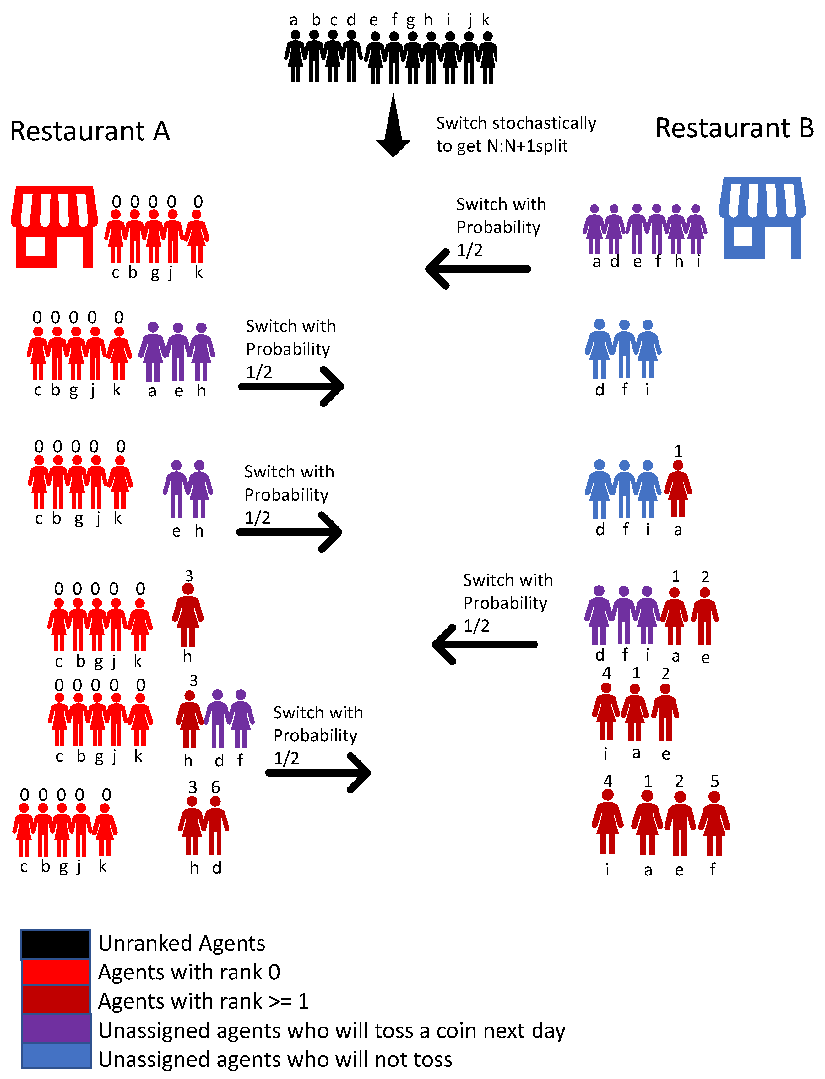
Let us consider an example for the case of say, agents in Figure 1. The agents are identified by the lower case letters . For example, at the end of the first stage, the agents have achieved the 5:6 split. Suppose agents are in restaurant A and the rest in B. Then, the agents in A are assigned ID 0, and know it. On the second day, Each of tosses a coin to decide to switch to the other restaurant or not. For example, get heads, and actually switch. At the end day, all agents know that three agents actually switched, and hence will be assigned one of the IDs from the set , and from the set . Then, on Day 3, and h toss a coin. For example, a gets head, and actually switches. Then, at the end of the day, it is known that a is assigned the ID 1. The next day, only e and h flip a coin, and rest stay with the previous days choice. If e actually jumps, then, at the end of day, everybody knows that IDs 2 and 3 have been assigned, and e knows that his is 2, and h knows that her ID is 3. The next day, and i toss coins, and the rest stay with their previous day’s choice, and so on.
5. Expected Time to Reach the Cyclic State
Firstly, we argue that the time required to complete the first stage, and assign rank zero to exactly N agents is of order . When the agents jump with probability on the first day, the expected number of agents in the first restaurant is , and standard deviation of this number is . Let us say that the number of people in the majority restaurant on any given day is . As the probability of jump is , with , the actual number of people jumping is a random variable, the distribution being approximately Poisson, with mean , and standard deviation approximately . Thus, we see that, on each day, the logarithm of deviation decreases to approximately half its value on previous day, until it becomes , and, after that, the expected time to reach split is finite. Thus, the total time to complete the first stage is , and may be neglected, for large N [13].
Now, we consider the time required for the second stage of the algorithm. Let the average time required to assign unique IDs in the second stage of the algorithm to a set of n agents be . Then, clearly, we have
We now show that . Note that, at the start of algorithm, both agents are in the same restaurant. Then, with probability , when both jump, they will end up in different restaurants, and the assignment is done. Else, with probability , both agents are in the same restaurant, and the state is the same as before. Hence, we must have
which implies that .
This argument is easily extended to higher values n. At the start, all n agents are in the same restaurant. Then, as each agent chooses to shift with probability , the probability that exactly r people shift is . However, then, the expected time for completion is . Taking into account the one extra day, we see that satisfies the linear equation
Since , this equation may be simplified to
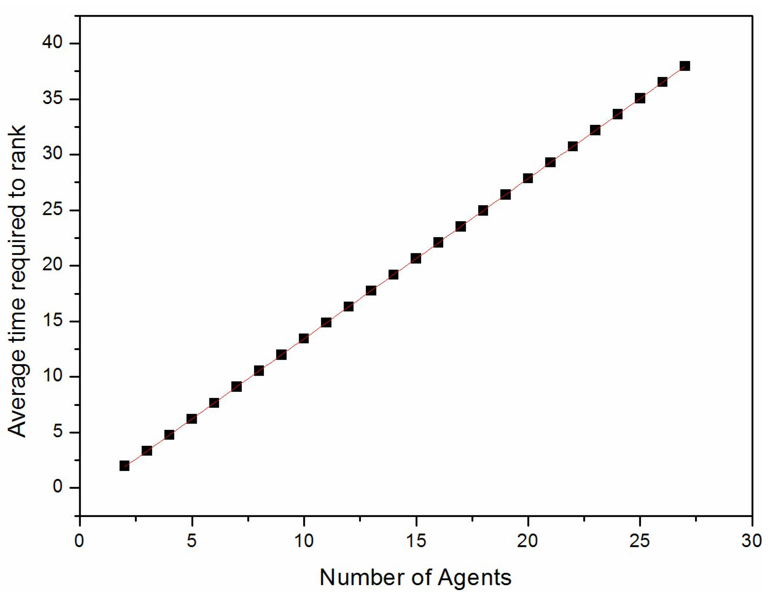
This is a linear equation that relates to values of , with . We can thus determine all the recursively. For example, we get , and . The resulting values of , for were determined numerically, using a simple computer program, and are shown in Figure 2. We see that increases approximately as .
Define the generating function
we see that satisfies the equation
We write , then the summation over s runs from 0 to , independent of the value of r, and, noting that , this can be done explicitly
Then, Equation (8) becomes
As a check, for small x, is approximately , which is consistent with above. For x near 1, we get , which implies that diverges as , for small . This then implies that varies linearly with n, for large n. To be more precise, we can find finite constants and such that .
We can simplify Equation (10) by making a change of variables . Then, in terms of the new variable y, we write
the equation for is seen to be
This equation is easily solved by iteration, giving
The asymptotic behavior of this function for y near 0 determines the behavior of , for x near 1. For very small y, we can extend the lower limit of summation in Equation (13) to . Then, the function tends to , which is defined by:
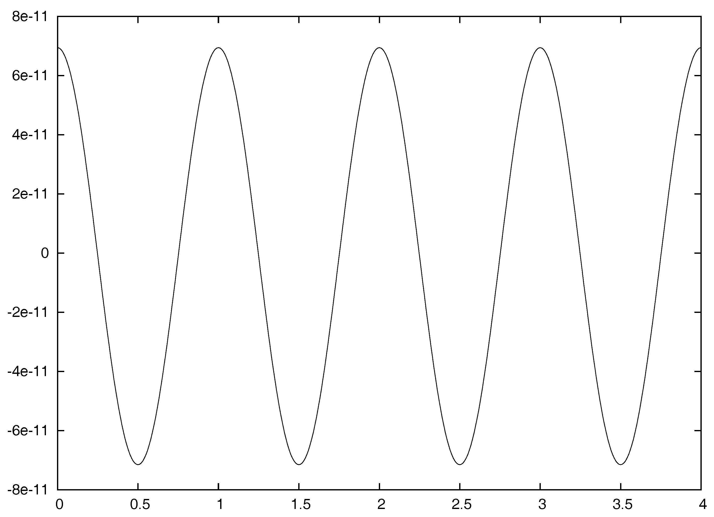
The function is clearly a log-periodic function of of period 1. A plot of this function is shown in Figure 3. We see that is nearly a constant, with value , but it has small oscillations of amplitude of order .
We note that remains bounded for all y, and hence varies as for . This implies that varies linearly with n for large n. In addition, log-periodic oscillations of with n correspond to log-periodic oscillations of with Y. Write
Then,
Using , we see that this gives
Define
Then, we have
Using Poisson summation formula, we have
where is the Fourier transform of defined as
It is easy to see that , which shows that . In Equation (20), we note that the integrand has simple poles in the complex-x plane at , for all integers n. For , we may close the contour from above. The residue at the poles is , which gives , and , which matches the numerically observed value of amplitude of the oscillations (Figure 2).
6. Summary and Concluding Remarks
In this paper, we have studied a version of the Minority game, where the agents try to coordinate their actions to get into a periodic state of period , in which every agent has the same long-time average payoff, and the global efficiency of the system is the maximum possible. We have proposed an algorithm that can achieve this aim in a time of order . We were able to determine the average running time of this algorithm exactly. As the time required to coordinate is of order N, the agents should have time horizon of at least order N, so that the cost of reaching the coordinated state is off-set by the slightly higher payoffs later.
As explained in the Introduction, we have assumed that the agents are rational, with unlimited memory, and use their full knowledge of efficiency of different strategies to decide what to do next. This is of course not realizable in practice. This work only provides the benchmark for measuring the performance of imperfect agents.
The question of how all agents decide about which strategy they will all use is clearly important. If we assume that all agents will use the strategy we have proposed, are we begging the question of establishing coordination amongst them? Our answer to this question may not be not fully convincing to all, and this issue perhaps needs further work. We have argued that the strategy we have proposed is distinguished by its simplicity, efficiency and analytical tractability.
Let us consider an alternate algorithm X that the agents could use to establish the periodic state. For the purpose of describing this algorithm, let us further assume that all agents have already somehow agreed that B is always the minority restaurant, and that they should use the natural choice of periodic sequence of length , with suitable phase shifts. The aim is to coordinate the choices of phase shifts so that the number of agents in B is exactly N on all days. However, now, the agents try to coordinate their phase shifts by trial and error. Then, initially, each chooses a phase shift at random, from 0 to . They use their phase-shifted sequence for days, and, at the end of this period, take stock of the attendance history of past days. If it is found that the restaurant A had more than people on some day r. The agent who was putting his phase shift starting at Day r, with a small probability, changes his phase shift to another day, randomly selected out of the days that showed less crowding. Then, they watch the performance over the next days, and again readjust phases again, until perfect coordination is achieved. It is easy to see that, while this will eventually find a cyclic state, the time required is much more than in our proposed strategy.
The problem of coordination amongst agents for optimal performance is also encountered in other games of resource allocation. For example, in the Kolkata Paise Restaurant problem [14,15], one has N agents, and N restaurants. The agents are all equal, and all of them agree to an agreed ranking of the restaurants (i.e., 1 to N). It is also given that each restaurant only serves one customer per day at a specially reduced price. Again, if the agents cannot communicate directly with each other in choosing which restaurant to go to, and they all want to avail of the special price, and also prefer to go to higher ranked restaurant, the optimal state where each agent can get a special price, and get to sample higher ranked restaurants as often as others, is the one where agents can organize themselves into a periodic state, where each agents visits restaurants ranked 1, 2, 3, and so on, on successive days, in a periodic way, and agents stagger the phases of their cycles so that every restaurant has exactly one visitor on each day. In this case, the problem of achieving the cyclic state may also be reduced to the problem of assigning each of N agents with a unique ID between 1 and N.
It is also straight forward to extend this algorithm to the El Farol Bar problem, where the two states are Go to bar, and Stay at home, and the payoff is 1 to agents who went to the bar, but only if the attendance at the bar is , where r is not restricted to be N. Then, the periodic state involving least number of switches is obtained when each agent goes to bar for r consecutive days, and stays at home for the next days, and the agent with ID j phase-shifts the origin of his cycle by amount j, .
Another point of interest in our results is the finding of log-periodic oscillations in the average time. Log-periodic oscillations have been seen in the analysis of several algorithms [9,10,11,16]. In most of these cases, the leading behavior is a simple power-law (or logarithmic dependence), and the log-periodic oscillations appear in the first correction to the asymptotic behavior [17]. In the problem studied here, the oscillations are seen in the coefficient of the variation of the leading linear dependence of average time of algorithm with number of agents.
The very small value of the amplitude of oscillations deserves some comment. Firstly, normally, one would expect this to be of , and explaining the origin of this “unnaturally small” value is of some theoretical interest. Here, we could calculate this amplitude exactly, but we do not know of any general argument to estimate even the order of magnitude of such amplitudes, without doing the exact calculation.
In systems with discrete scale invariance, such as deterministic fractals, amplitudes of order have been seen [18,19]. However, even in these cases, where log-periodic oscillations are rather expected, they only form the sub-leading correction: for example, in the case of number rooted of polygons of length n on fractals, we get has a part that grows as , and then there is an additive log-periodic oscillatory term of finite amplitude [18]. The log-periodic oscillations in in this paper come in a multiplicative term, and hence the amplitude will grow with n, for large n.
Author Contributions
D.D. supervised the project and contributed towards the conceptualization of the proposed strategy, analysis and the overall writing, reviewing and editing process. H.R. contributed towards the conceptualization, formal analysis, data visualization and the overall writing, reviewing and editing process.
Acknowledgments
Hardik Rajpal thanks Tata Institute of fundamental Research, Mumbai for hosting his visit in the summer of 2016, and Indian Institute of Science Education and Research, Pune, for support in the summer of 2017, which made this work possible. We thank V. Sasidevan and R. Dandekar their comments on the draft manuscript. Deepak Dhar’s work is supported in part by the J. C. Fellowship, awarded by the Department of Science and Technology, India, under the grant DST-SR-S2/JCB-24/2005.
Conflicts of Interest
The authors declare no conflict of interest.
References and Note
- Challet, D.; Zhang, Y.C. Emergence of cooperation and organization in an evolutionary game. Phys. A Stat. Mech. Appl. 1997, 246, 407–418. [Google Scholar] [CrossRef]
- Moro, E. Minority Games: An introductory guide. In Advances in Condensed Matter and Statistical Physics; Korutcheva, E., Cuerno, R., Eds.; Nova Science Publishers: Hauppauge, NY, USA, 2004; pp. 263–286. [Google Scholar]
- Kets, W. Learning with Fixed Rules: The Minority Game. J. Econ. Surv. 2011, 26, 865–878. [Google Scholar] [CrossRef]
- Challet, D.; Marsili, M.; Zhang, Y.C. Minority Games; Oxford University Press: Oxford, UK, 2005. [Google Scholar]
- Challet, D.; Coolen, A.C.C. The Mathematical Theory of Minority Games. Statistical Mechanics of Interacting Agents. J. Econ. 2006, 88, 311–314. [Google Scholar] [CrossRef]
- Sasidevan, V.; Dhar, D. Strategy switches and co-action equilibria in a minority game. Phys. A Stat. Mech. Appl. 2014, 402, 306–317. [Google Scholar] [CrossRef]
- Crawford, V.P. Adaptive Dynamics in Coordination Games. Econometrica 1995, 63, 103. [Google Scholar] [CrossRef]
- Samuel, J.; Sinha, S. Surface tension and the cosmological constant. Phys. Rev. Lett. 2006, 97, 161302. [Google Scholar] [CrossRef] [PubMed]
- Sedgewick, R.; Flajolet, P. An Introduction to the Analysis of Algorithms; Addison Wesley: Boston, MA, USA, 2013. [Google Scholar]
- Prodinger, H. Periodic Oscillations in the Analysis of Algorithms and Their Cancellations. J. Iran. Stat. Soc. 2004, 3, 251–270. [Google Scholar]
- Odlyzko, A. Periodic oscillations of coefficients of power series that satisfy functional equations. Adv. Math. 1982, 44, 180–205. [Google Scholar] [CrossRef]
- Satinover, J.B.; Sornette, D. “Illusion of control” in Time-Horizon Minority and Parrondo Games. Eur. Phys. J. B 2007, 60, 369–384. [Google Scholar] [CrossRef]
- Dhar, D.; Sasidevan, V.; Chakrabarti, B.K. Emergent cooperation amongst competing agents in minority games. Phys. A Stat. Mech. Appl. 2011, 390, 3477–3485. [Google Scholar] [CrossRef]
- Chakrabarti, A.S.; Chakrabarti, B.K.; Chatterjee, A.; Mitra, M. the Kolkata Paise Restaurant problem and resource utilization. Phys. A Stat. Mech. Appl. 2009, 388, 2420–2426. [Google Scholar] [CrossRef]
- Chakrabarti, B.K.; Chatterjee, A.; Ghosh, A.; Mukherjee, S.; Tamir, B. Econophys. of the Kolkata Restaurant Problem and Related Games; Springer: Heidelberg/Berlin, Germany, 2017. [Google Scholar]
- Geraskin, P.; Fantazzini, D. Everything you always wanted to know about log-periodic power laws for bubble modeling but were afraid to ask. Eur. J. Financ. 2013, 19, 366–391. [Google Scholar] [CrossRef] [Green Version]
- We are thankful to Prof. J. Radhakrishnan for this observation.
- Sumedha; Dhar, D. Quenched Averages for Self-Avoiding Walks and Polygons on Deterministic Fractals. J. Stat. Phys. 2006, 125, 55–76. [Google Scholar] [CrossRef]
- Akkermans, E.; Benichou, O.; Dunne, G.V.; Teplyaev, A.; Voituriez, R. Spatial log-periodic oscillations of first-passage observables in fractals. Phys. Rev. E 2012, 86. [Google Scholar] [CrossRef] [PubMed]
Figure 1.
Ranking of N = 11 agents using the proposed algorithm. The numerals above the agents indicates their assigned IDs.
Figure 1.
Ranking of N = 11 agents using the proposed algorithm. The numerals above the agents indicates their assigned IDs.

Figure 2.
Numerically determined exact values of for . The equation of the approximate linear fit here is .
Figure 2.
Numerically determined exact values of for . The equation of the approximate linear fit here is .

Figure 3.
Log-periodic oscillations in the function as a function of , determined by numerically summing the series in Equation (14), about the mean value . Note the small amplitude of the oscillations.
Figure 3.
Log-periodic oscillations in the function as a function of , determined by numerically summing the series in Equation (14), about the mean value . Note the small amplitude of the oscillations.

© 2018 by the authors. Licensee MDPI, Basel, Switzerland. This article is an open access article distributed under the terms and conditions of the Creative Commons Attribution (CC BY) license (http://creativecommons.org/licenses/by/4.0/).
Share and Cite
MDPI and ACS Style
Rajpal, H.; Dhar, D. Achieving Perfect Coordination amongst Agents in the Co-Action Minority Game. Games 2018, 9, 27. https://doi.org/10.3390/g9020027
AMA Style
Rajpal H, Dhar D. Achieving Perfect Coordination amongst Agents in the Co-Action Minority Game. Games. 2018; 9(2):27. https://doi.org/10.3390/g9020027
Chicago/Turabian StyleRajpal, Hardik, and Deepak Dhar. 2018. "Achieving Perfect Coordination amongst Agents in the Co-Action Minority Game" Games 9, no. 2: 27. https://doi.org/10.3390/g9020027
Note that from the first issue of 2016, this journal uses article numbers instead of page numbers. See further details here.