
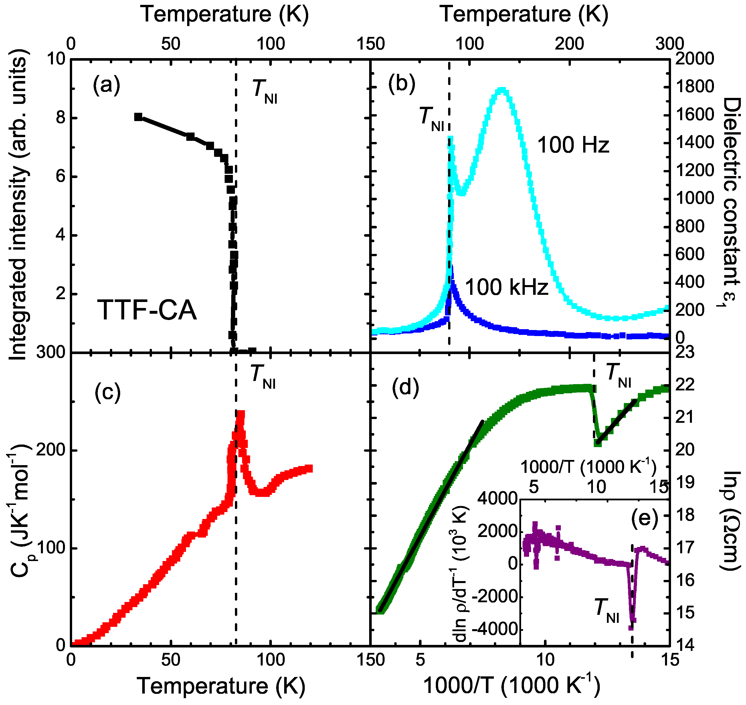
Infrared Investigations of the Neutral-Ionic Phase Transition in TTF-CA and Its Dynamics


Abstract
:1. Introduction
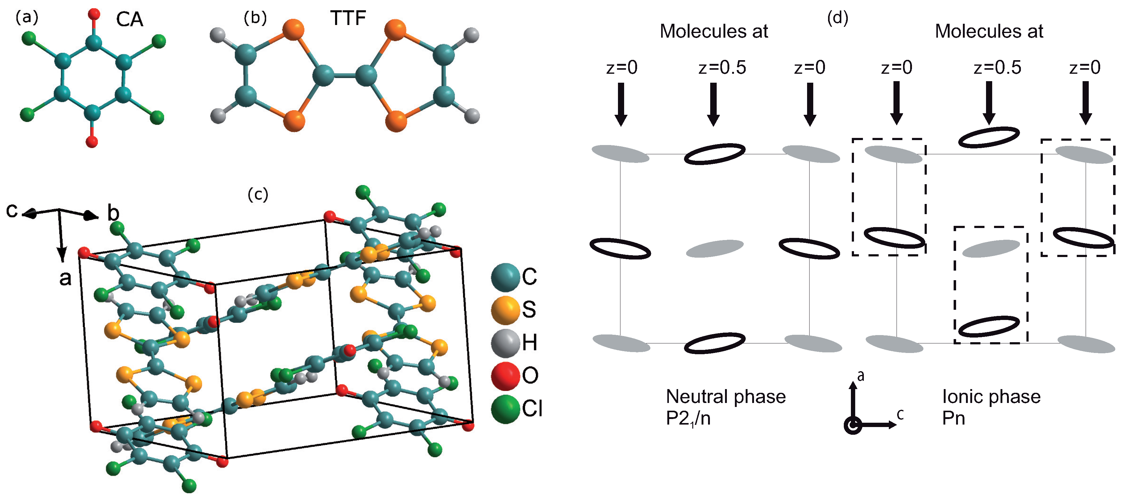
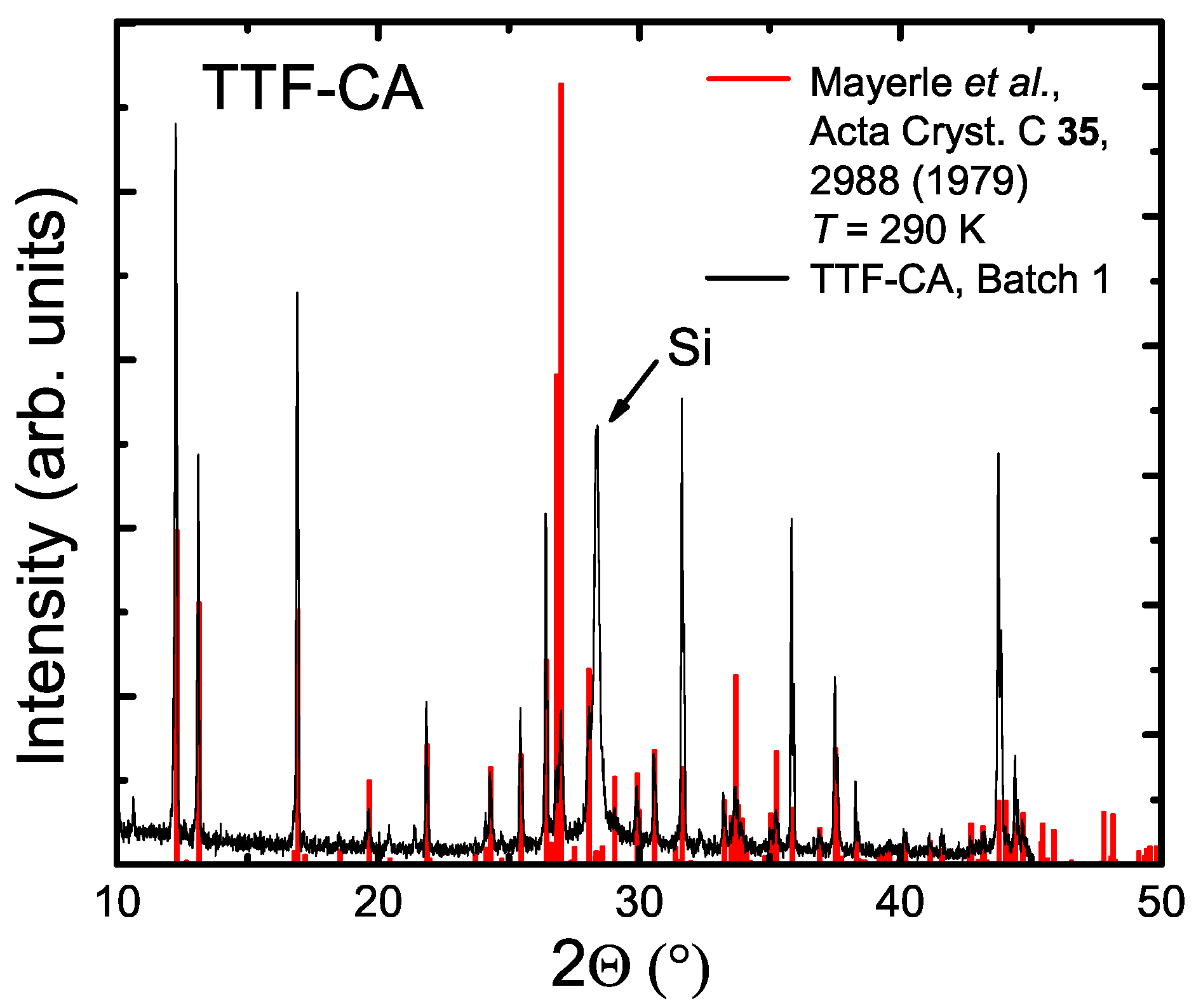
2. Crystal Growth
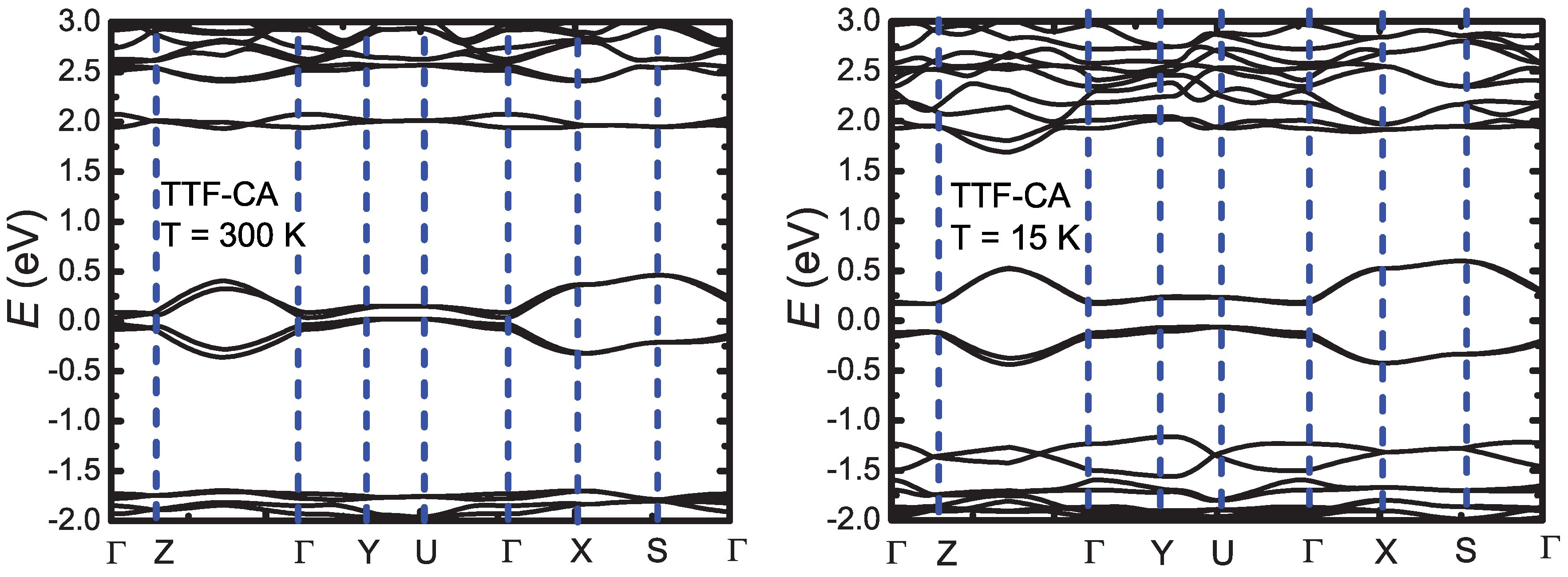
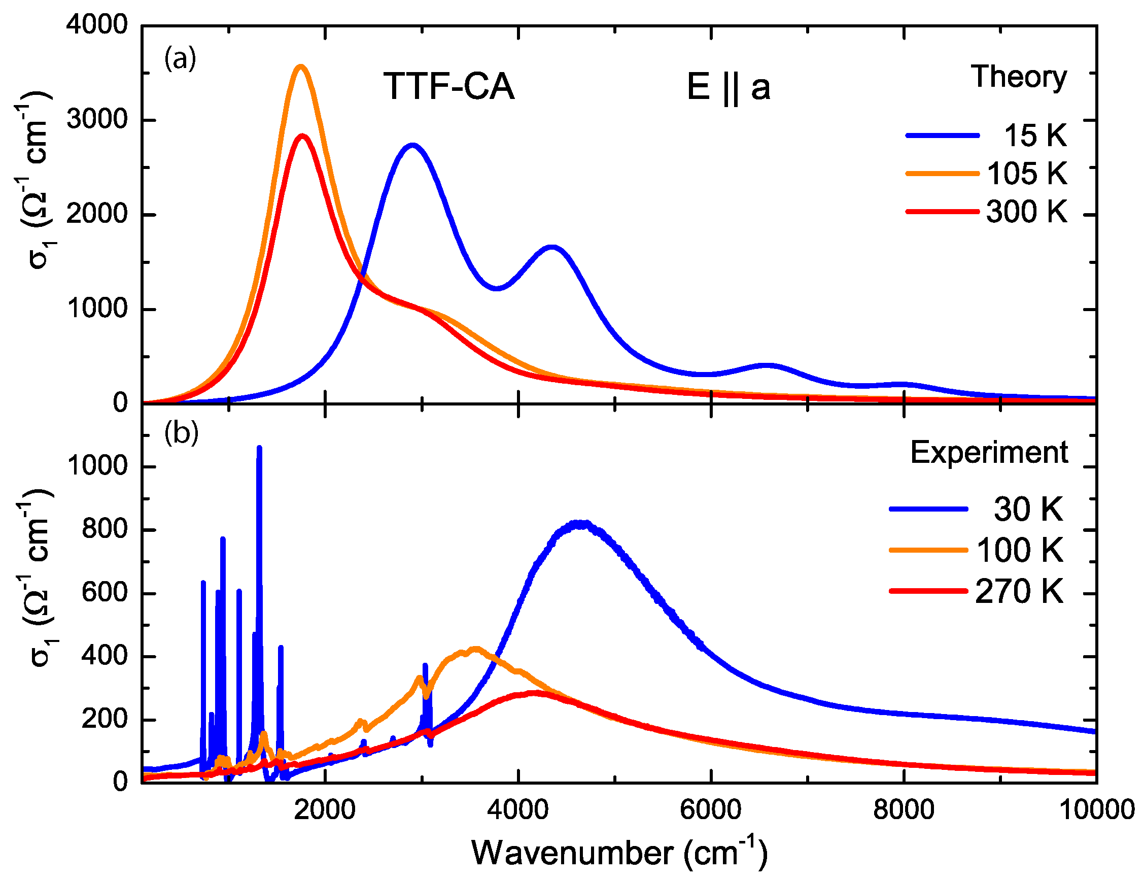
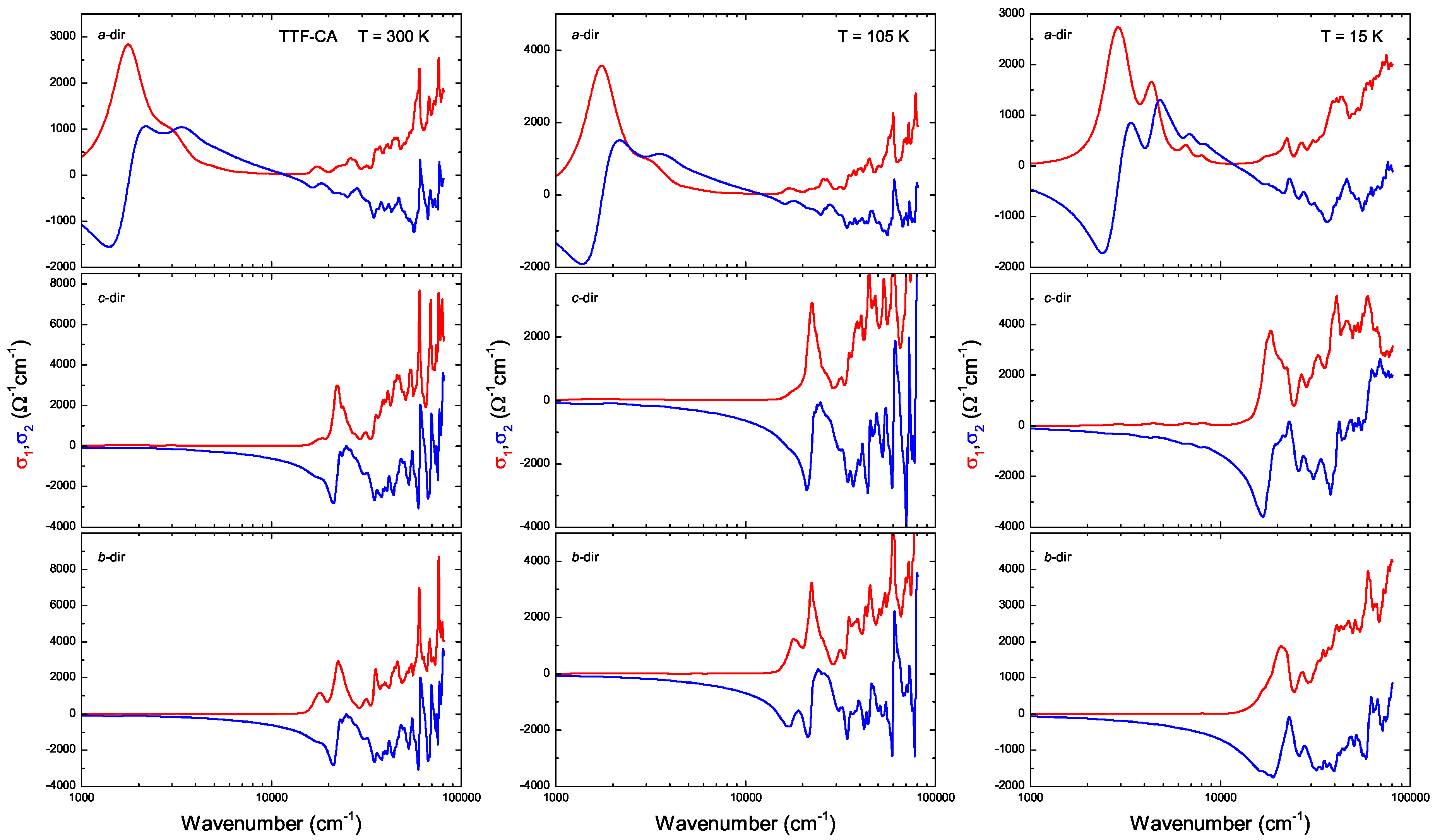
3. Ab-Initio Calculations: Band Structure, Optical Spectra and Normal Modes
4. Infrared Measurements
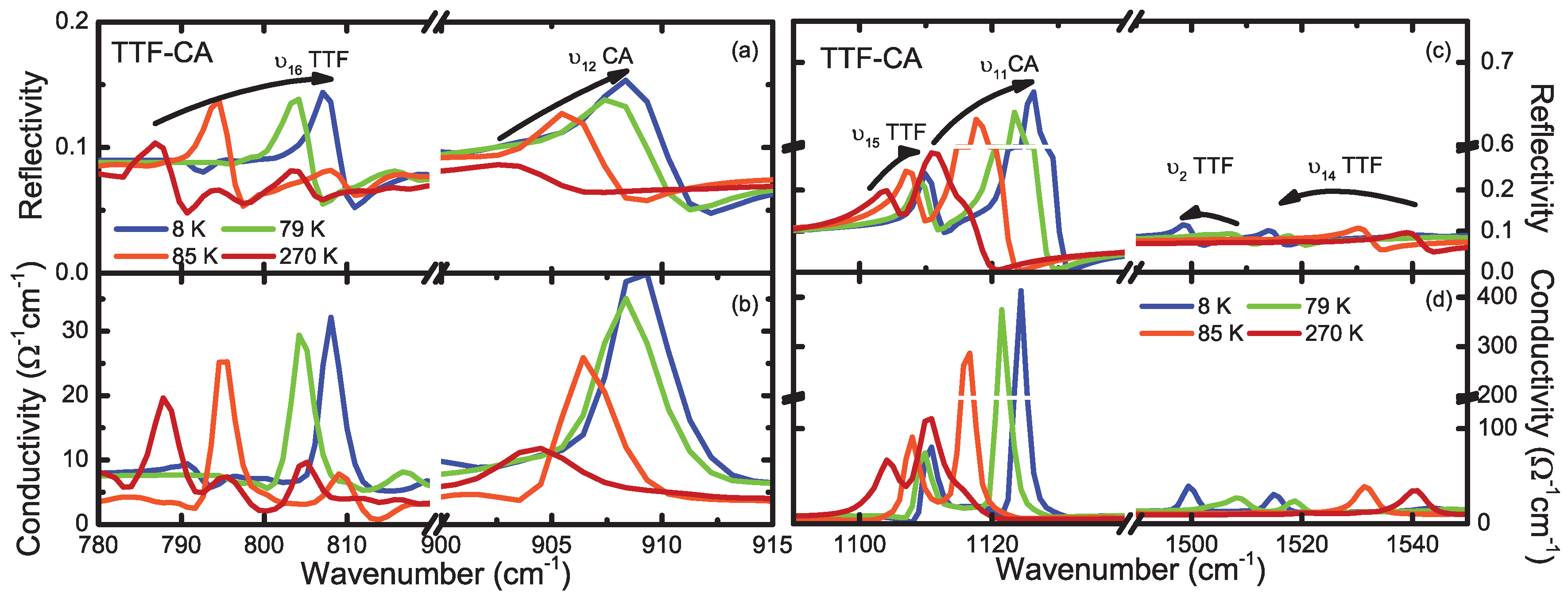
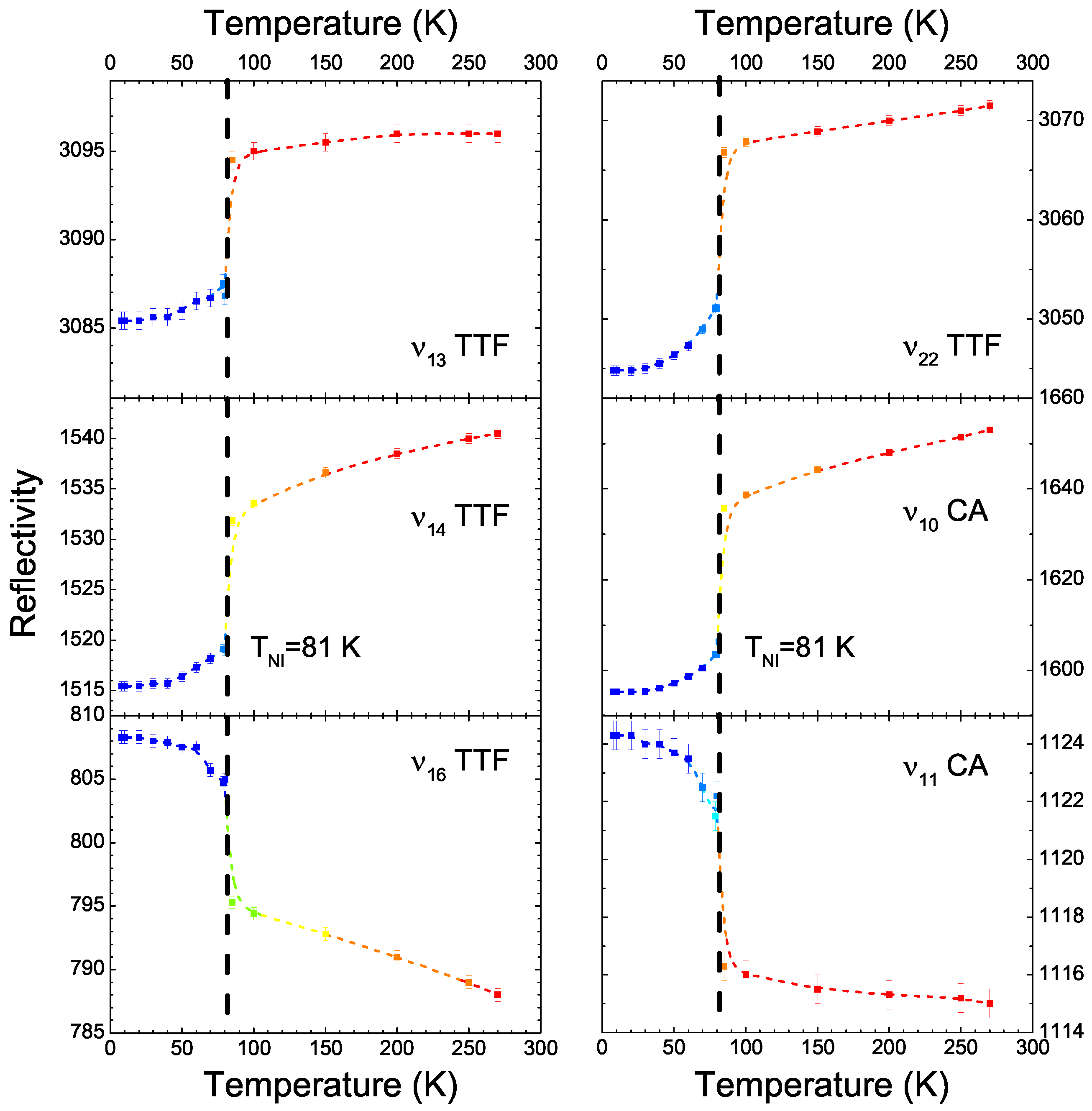
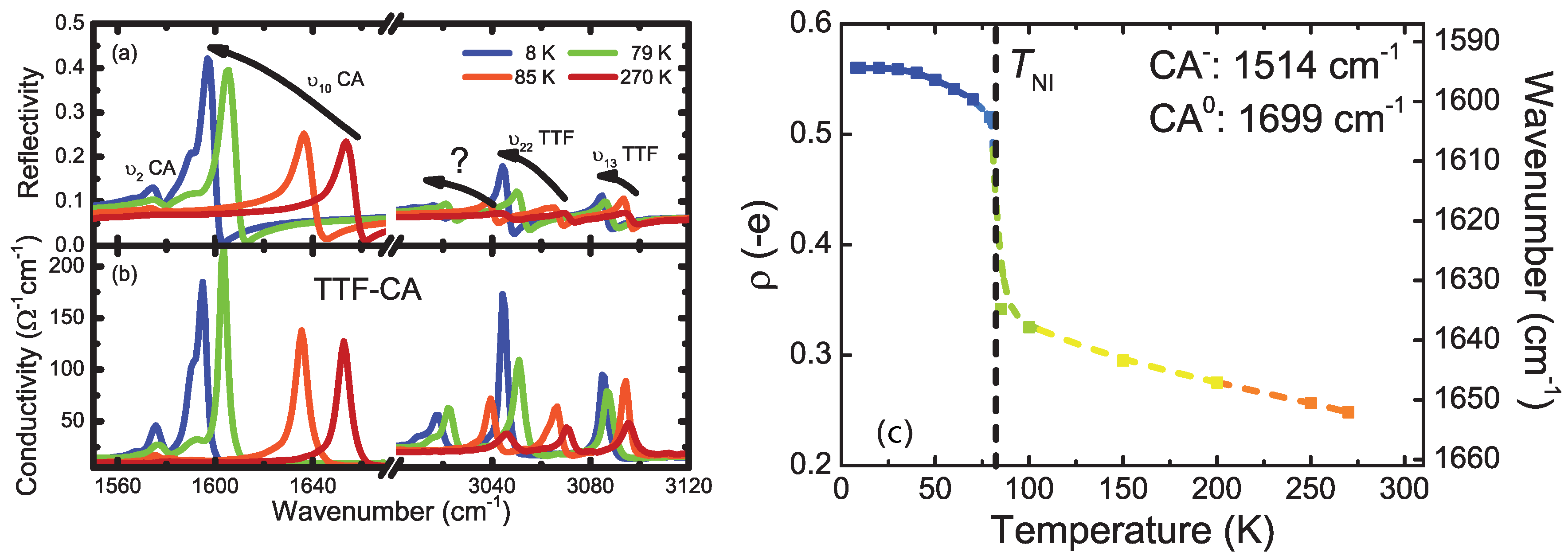
4.1. b-Direction
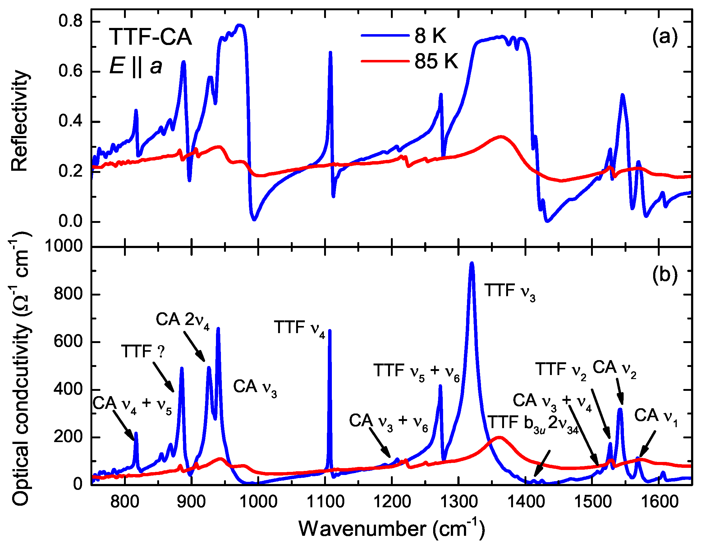
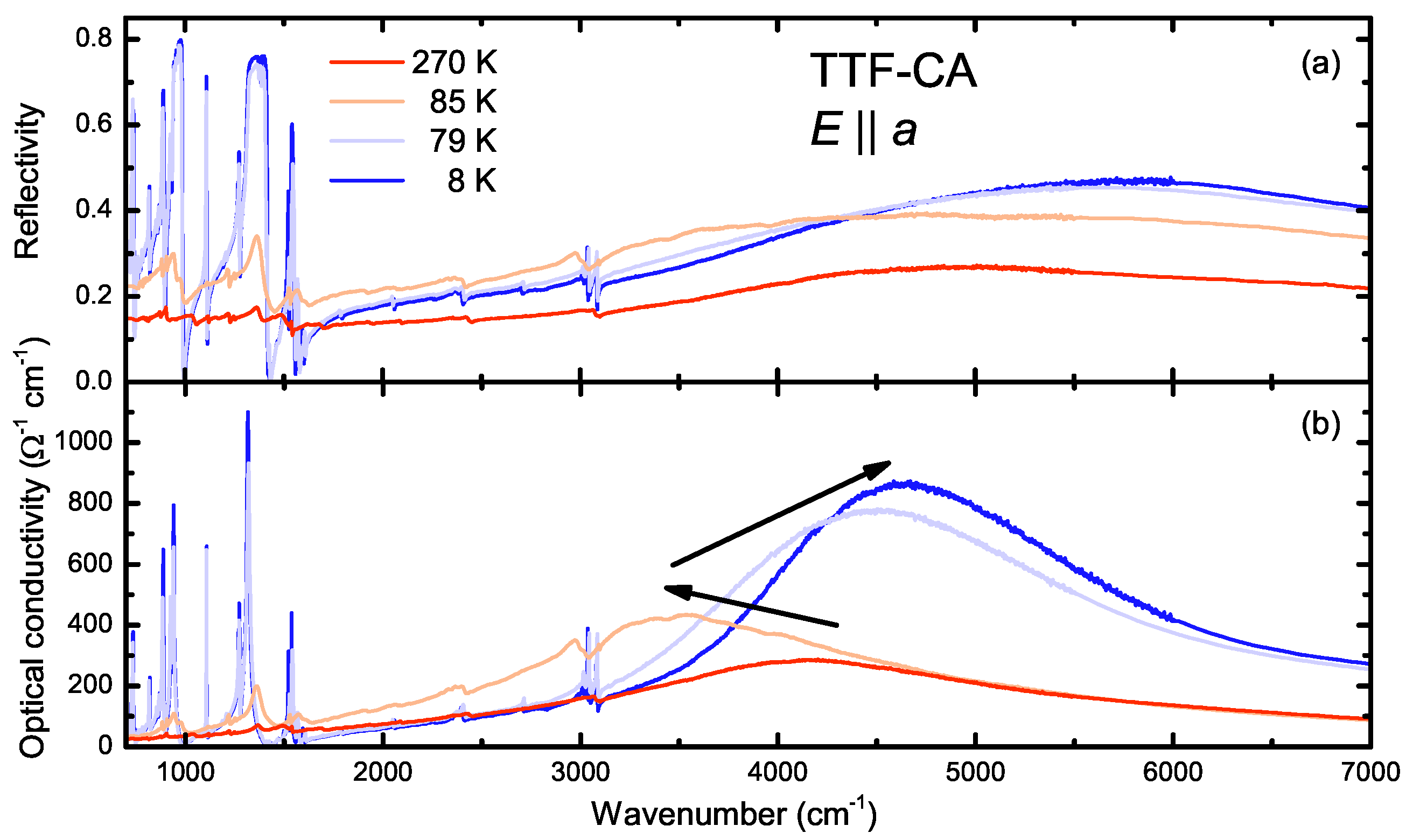
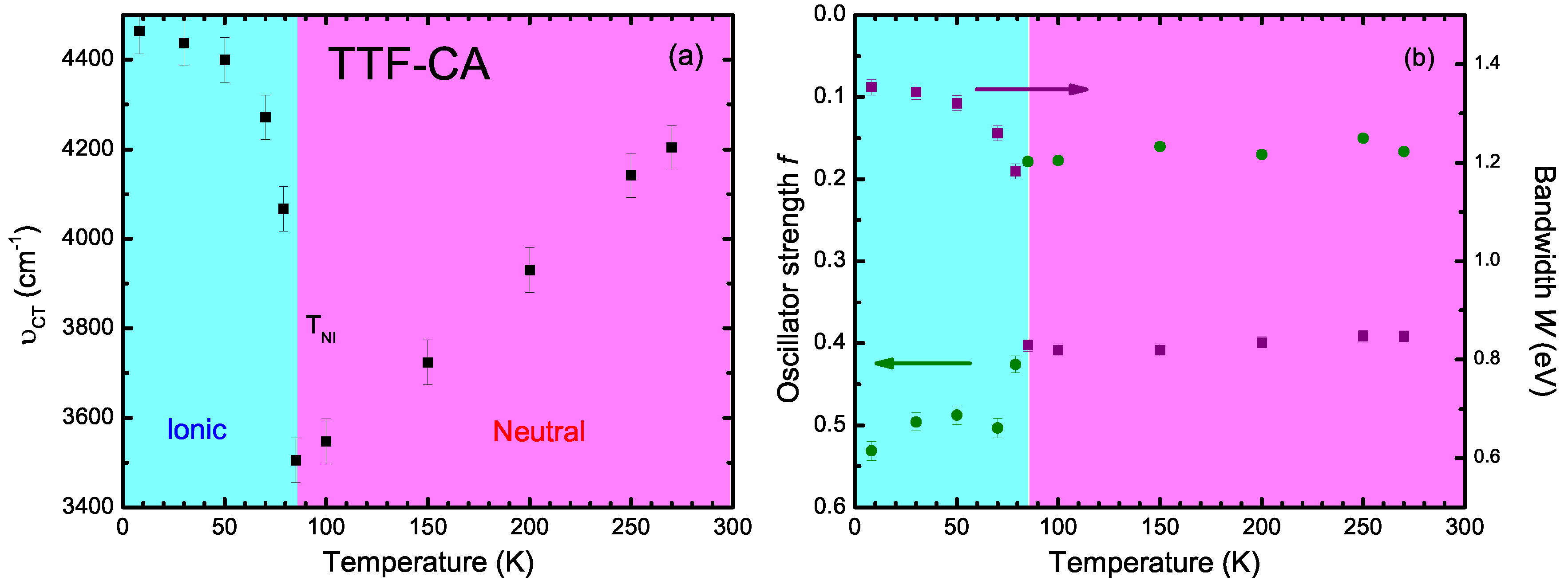
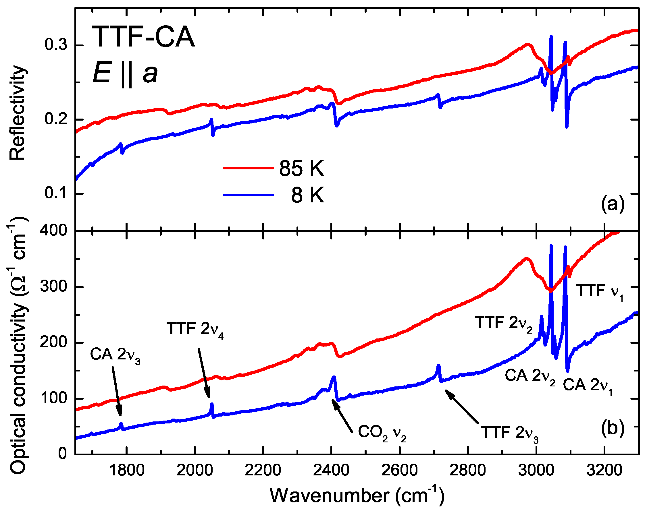
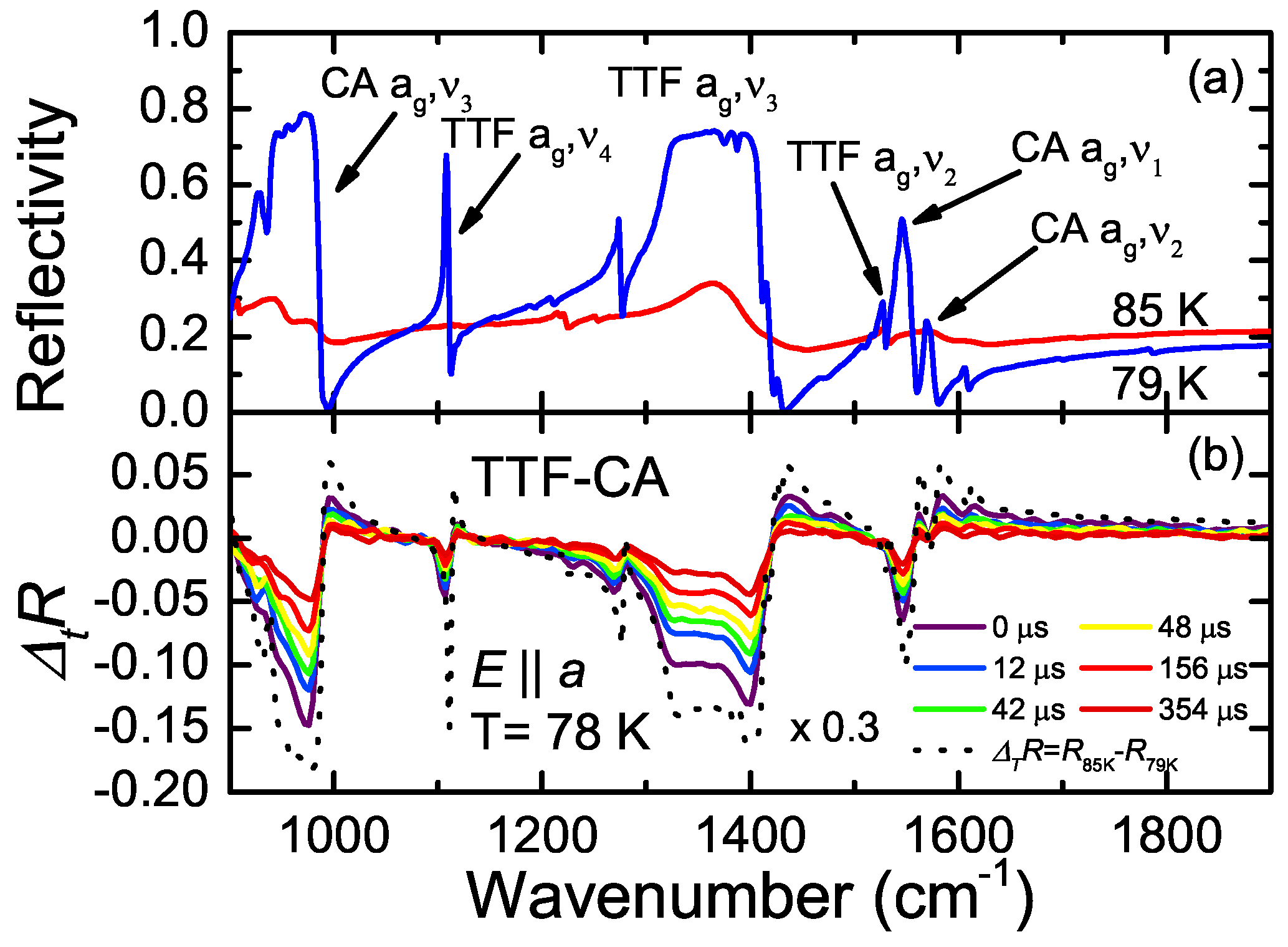
4.2. a-Direction
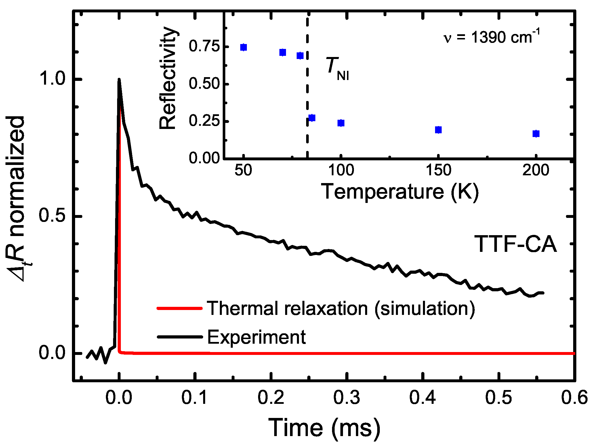
5. Photo-Induced Phase Transition in TTF-CA
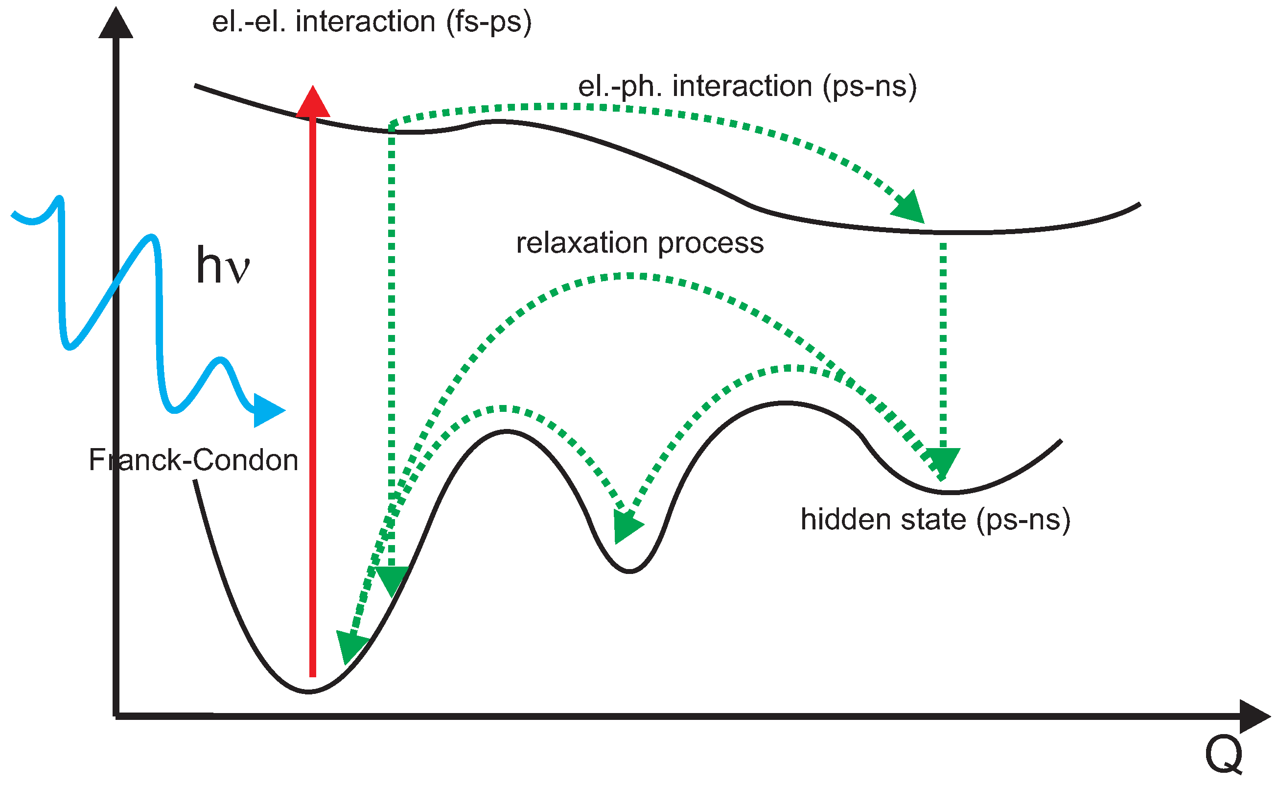
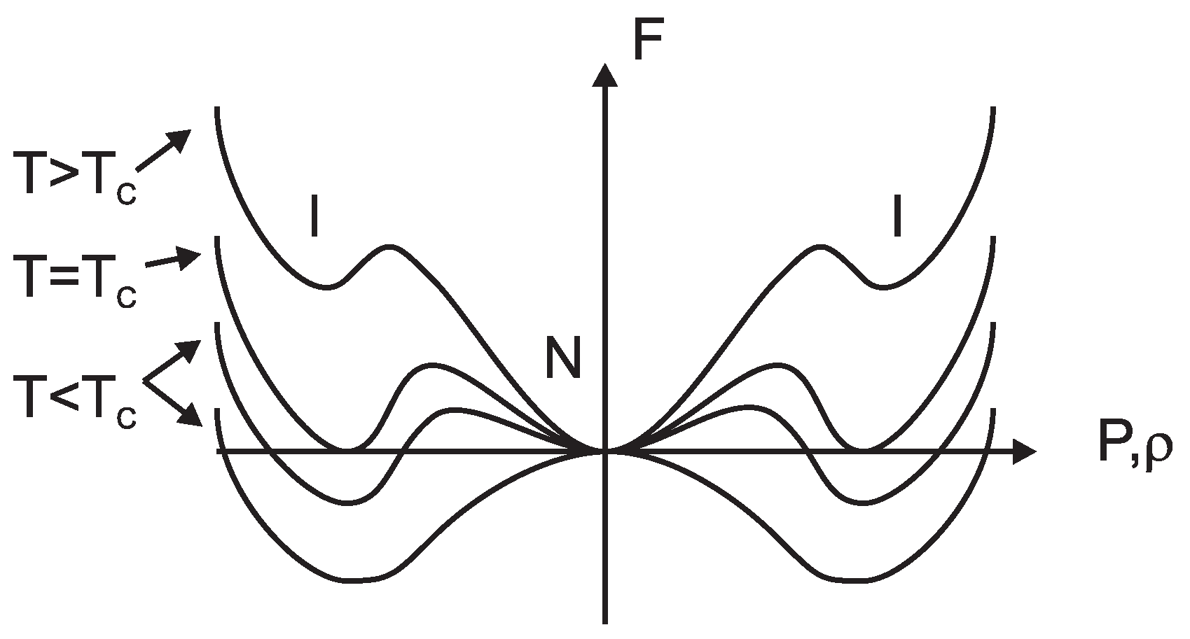
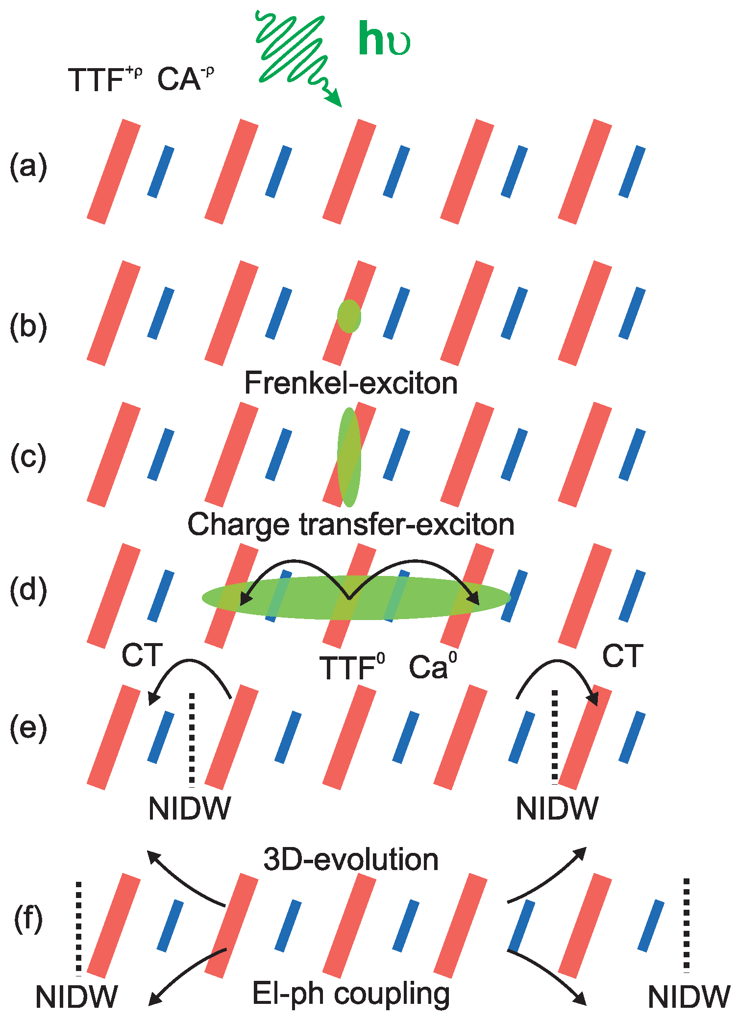
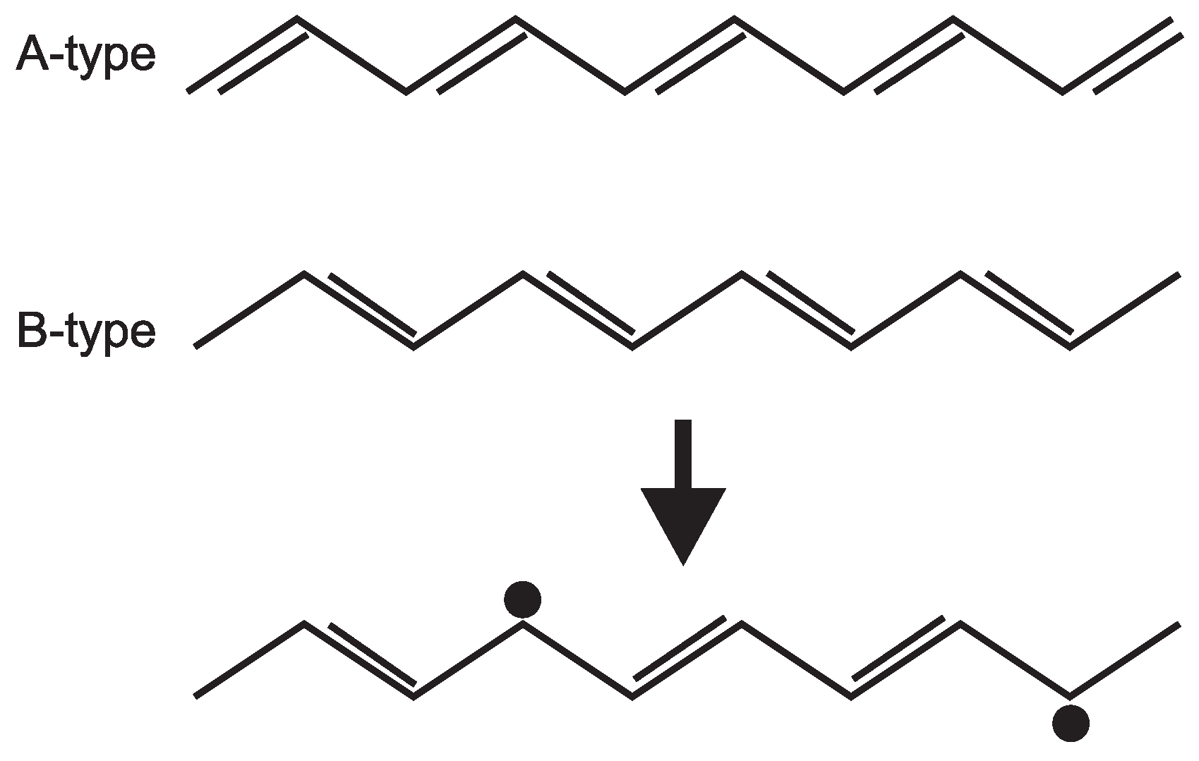
5.1. Underlying Principle
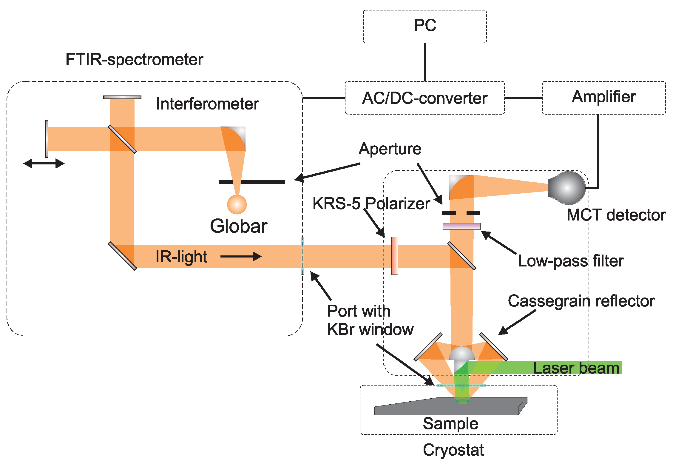
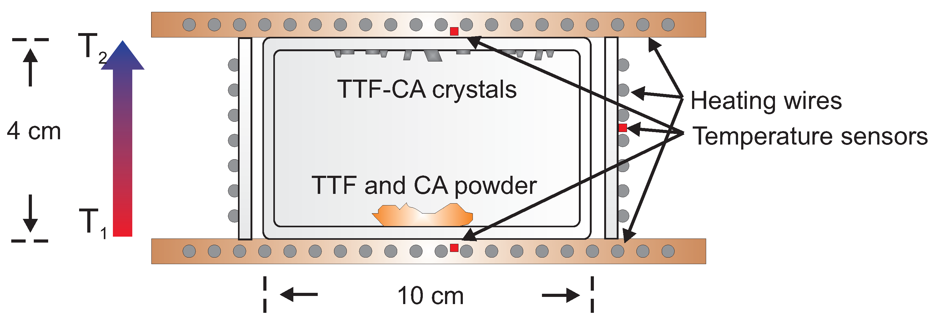
5.2. Experimental Configuration
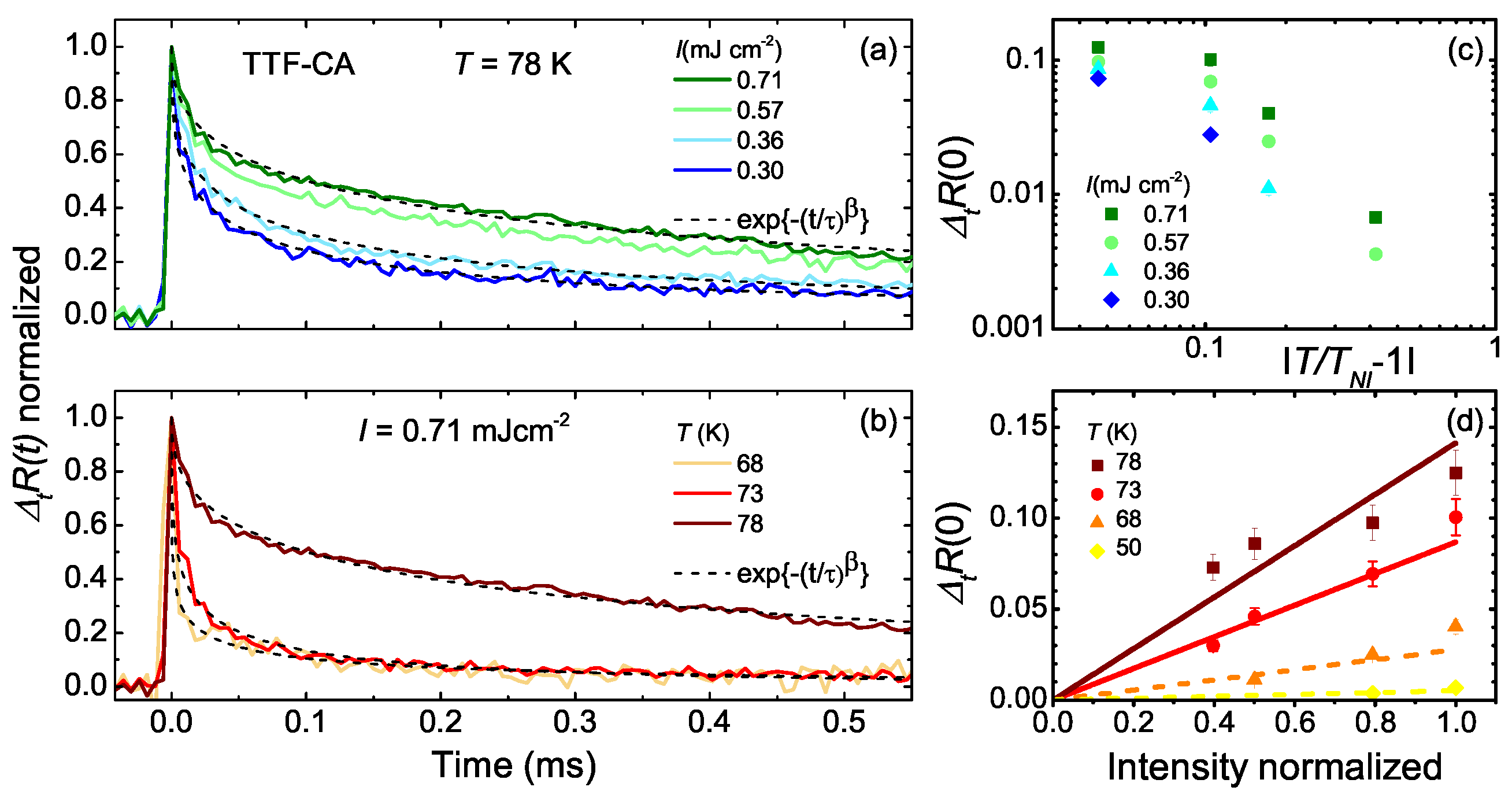
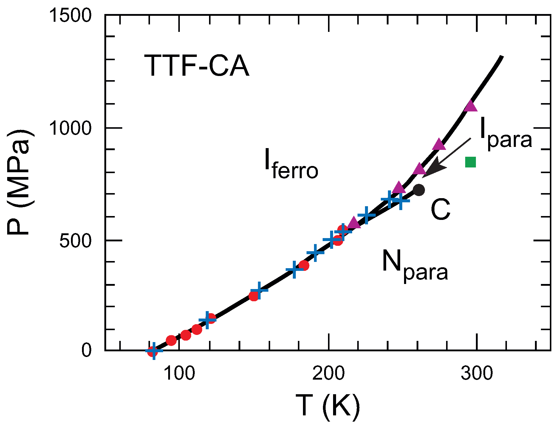
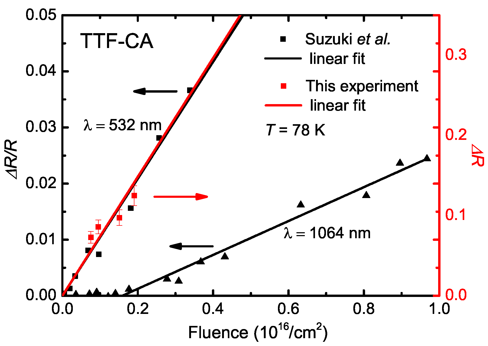
5.3. Photo-Induced Phase Transition
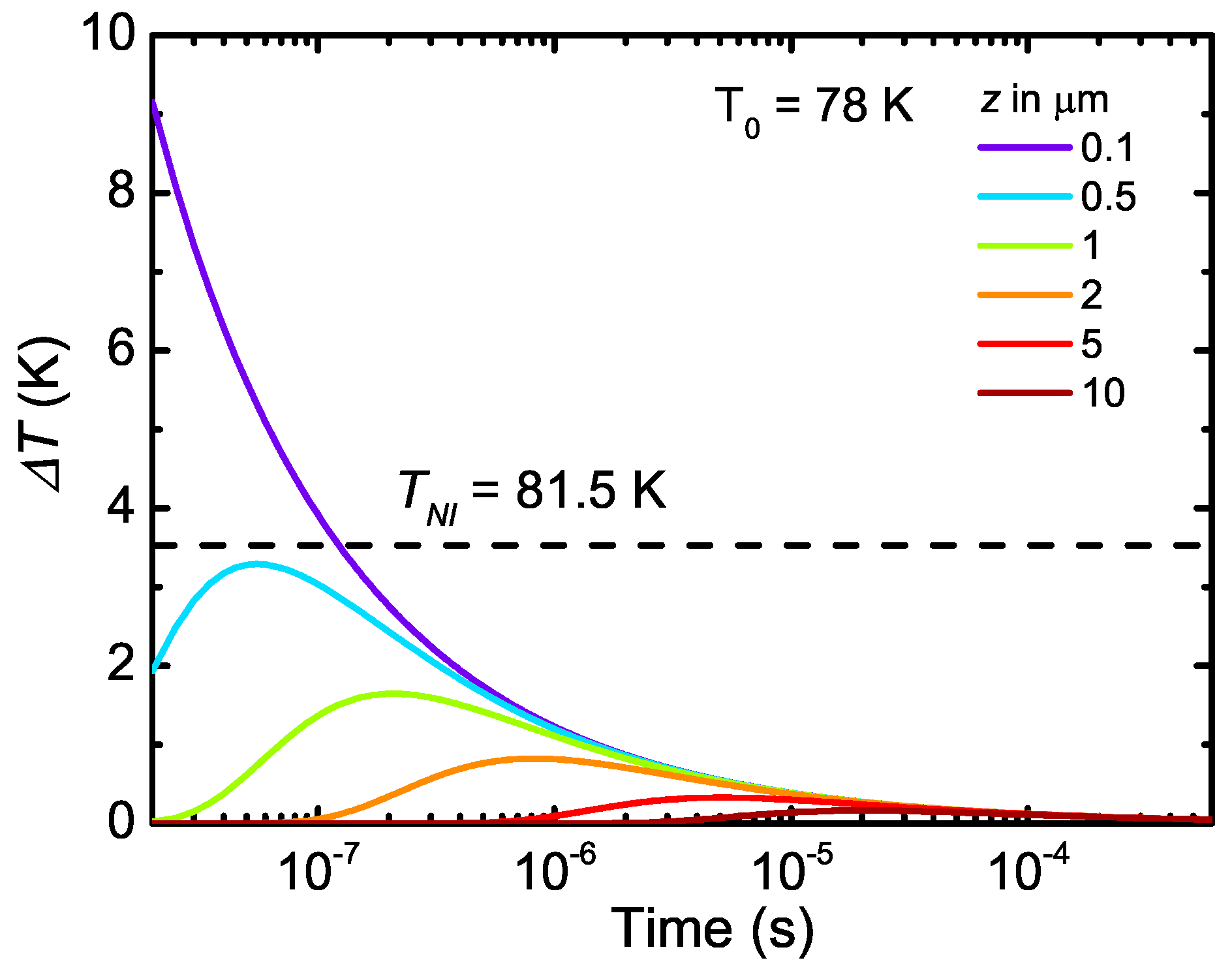
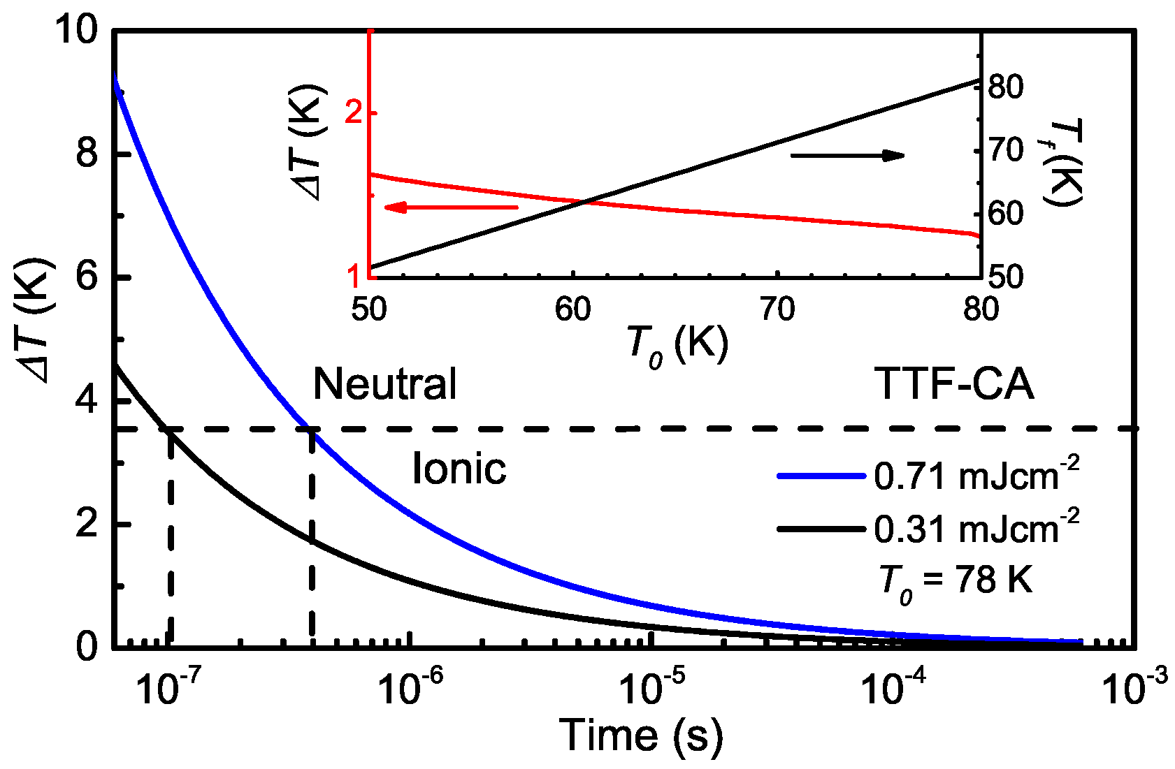
5.4. Heating Effect
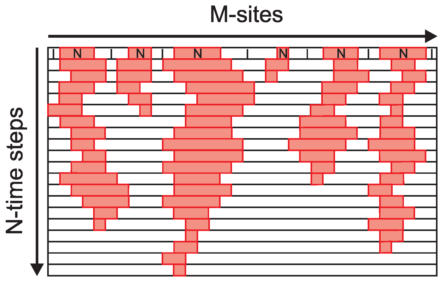
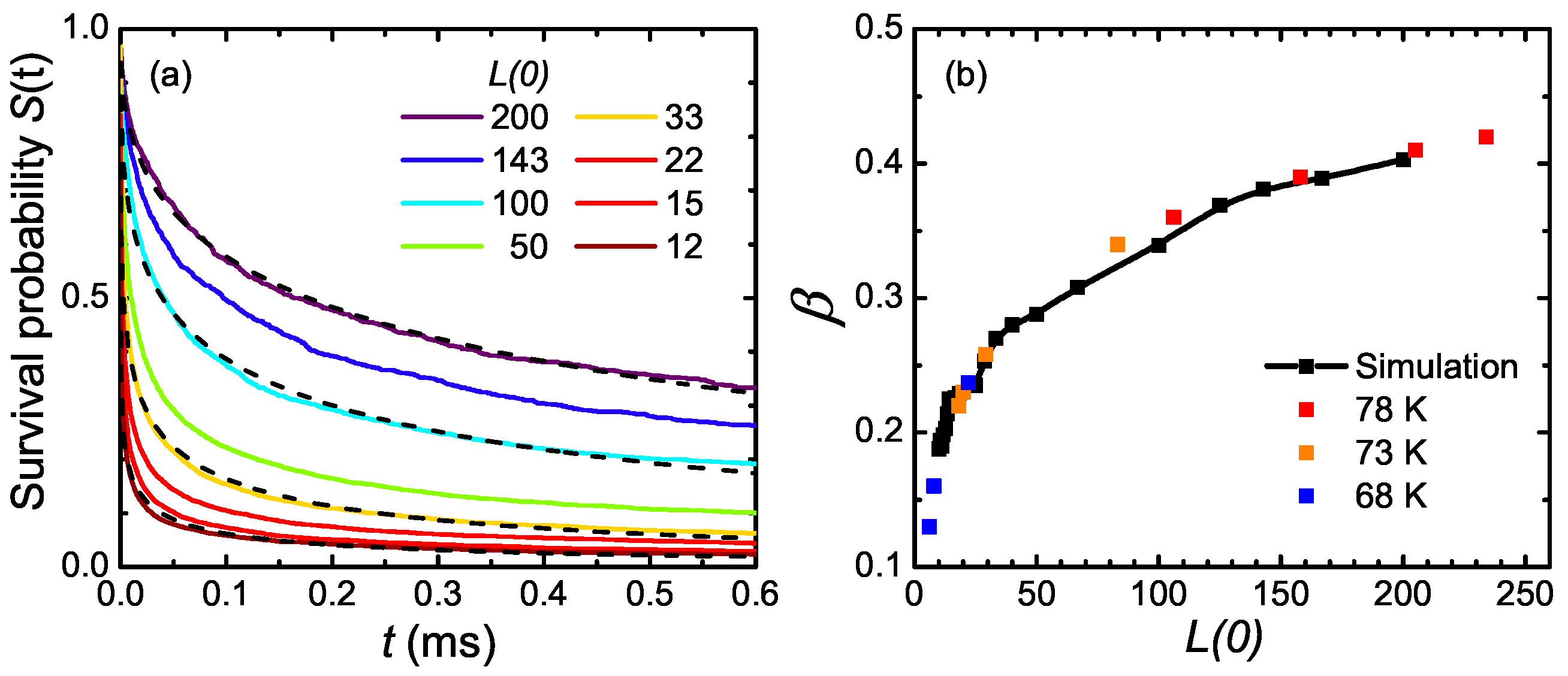
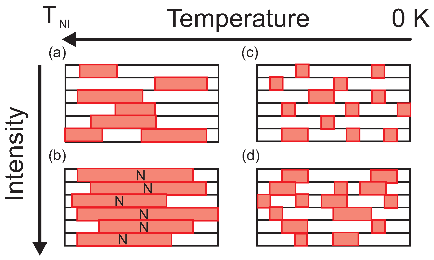
6. One-Dimensional Random Walk: Electronically Driven Transition
7. Conclusions
Acknowledgments
Author Contributions
Conflicts of Interest
Appendix A. Light-Matter Interaction
Appendix A.1. Drude Model
Appendix A.2. Drude–Lorentz Model
Appendix A.3. Fano Model
Appendix B. Theoretical Calculations
Appendix B.1. Band Structure and Optical Functions
Appendix B.1.1. Functional
- Level 1: the most famous is the so-called local density approximation (LDA) or local spin density approximation (LSDA) functional. It is assumed that corresponds to the known exchange-correlation energy of a homogeneous electron gas, which is directly related to the electron density. LDA describes metallic systems very well as they can be approximated by an undisturbed electron gas. However, it fails to model systems in which the electron density strongly varies in space, such as semiconductors or insulators.
- Level 2: a significant improvement of the precision and results is achieved by taking into account the spatial variation of the electron density. It can be considered as an additional correction parameter for LSDA. These functionals are summarized under the keyword: generalized gradient approximation (GGA). The most famous GGA functionals are B88 [122], BLYP [123], PW91 [124], and Perdew–Burke–Enzerhof (PBE) [52,125].
- Level 3: when higher derivatives of the electron density are included, they are called meta-GGA functionals.
- Level 4: furthermore, hybrid-GGA functionals are used to describe atoms as well as molecules with a much higher precision. Different exchange and correlation functionals are mixed and combined with each other depending on their coefficient. If they are determined by fitting experimental data, they are called semi-empirical functionals, or they have to satisfy certain predefined conditions. The most used representatives are B3LYP [126,127,128], and PBE1PBE [129] functionals. For more detail, it is referred to the relevant literature [130].
- Level 5: radom phase approximation (RPA).
Appendix B.1.2. Basis Set
- One possibility is to start with localized orbitals that can be divided in two subgroups: Slater-orbitals and Gauss-orbitals. Considering only the last ones, they are built of polynomial functions multiplied with Gaussian functions (exp). The main advantage of this mathematical construction is that the matrix element, i.e., integrals, can be solved analytically and hence, computing time can be reduced. The precision can be increased by enlarging the size of the basis function. Furthermore, diffuse and polarization function can be added to the standard basis set because they describe molecular bonds and charged states of molecules much better.The Gaussian or Pople basis sets are mainly used for calculations of isolated molecules or structures, because the wave functions decay with increasing distance to the atom or molecule and thus the electron density is only calculated where also charge is present. In addition, a Gaussian basis set also describes the region close to the nucleus rather well.
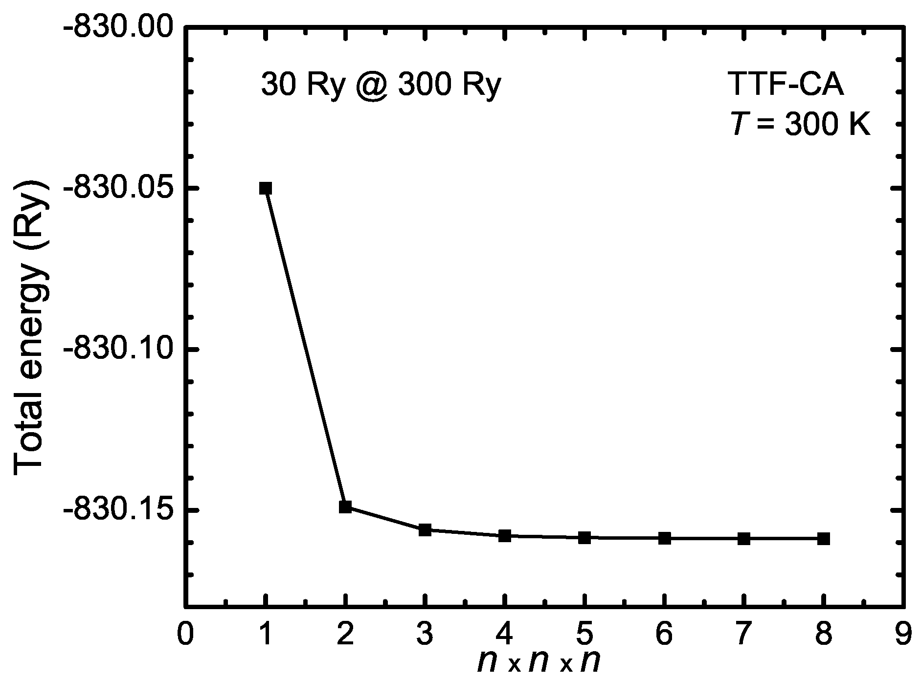
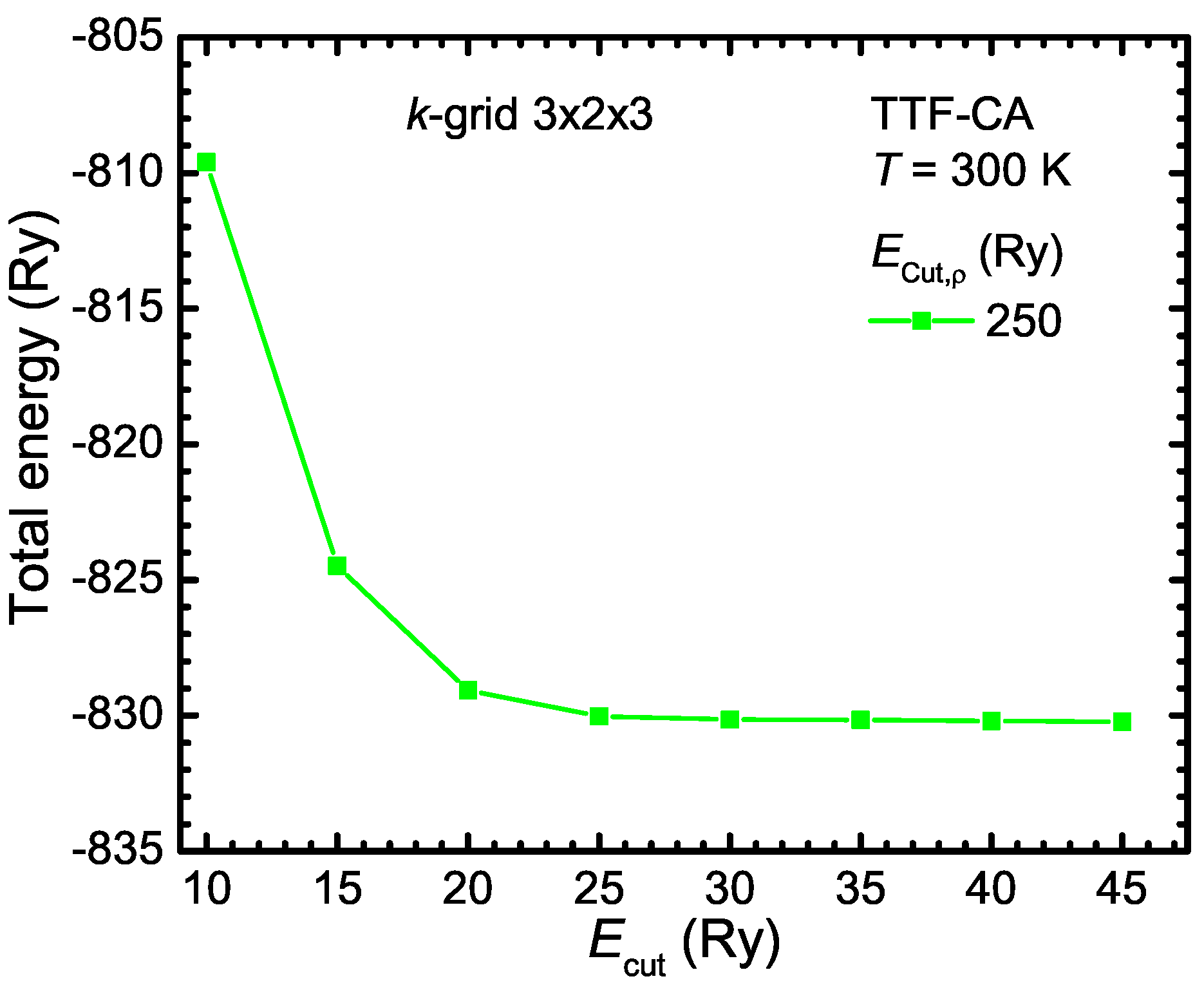
- Instead of approximating the wave functions by a linear combination of Gaussian functions, they can be constructed from the linear combinations of plane waves:This construction is perfectly suitable for the description of any periodic crystal structure. Typically, the valence electrons are responsible for the bindings and the core electrons can be regarded as an additional correction. Since close to the atomic cores the wave function oscillates very strongly, they have to be described by large wave vectors . According to Schrödinger’s Equation (B2), the kinetic energy of the electrons is a quadratic function of the -vector. Therefore, the kinetic energy of the core electrons is very large. This leads to an extremely large number of wave functions, in general, and makes it necessary to define a cutoff energy of the electrons in consideration the required precision. Thus, to limit the number of wave functions, the pure atomic potential is approximated by a pseudo potential.The minimum cutoff-energy must be identified in respect to the total energy of the system. In Figure B1, the total energy of the organic compound TTF-CA is plotted as a function of the wave function cutoff energy for a cutoff energy of the electron density of 250 Ry. For the convergence test, ultrasoft pseudo potentials were used (see for more details the following Appendix B.1.3). Above Ry, the total energy converges and does not change significantly anymore. Therefore, Ry is a good value for the calculations. The cutoff energy of the electron density should be by a factor of four larger than for norm-conserving pseudo potential In the case of ultrasoft pseudo potential, must be between 8 and 12 times larger than .Moreover, the number of plane waves depends on the maximal defined kinetic energy and the volume of the unit cell . Note, the volume of the plane waves in the reciprocal space is at which the volume of a single plane wave is . Hence, the necessary number of wave functions increases with increasing the unit cell size and is much larger in contrast to the localized approach with Gaussian functions, for instance. However, plane waves can also be used for isolated molecules, but for this purpose a very large super cell has to be defined so that the plane waves decay very fast within the cell and do not interact with their mirror image of the neighboring cells.

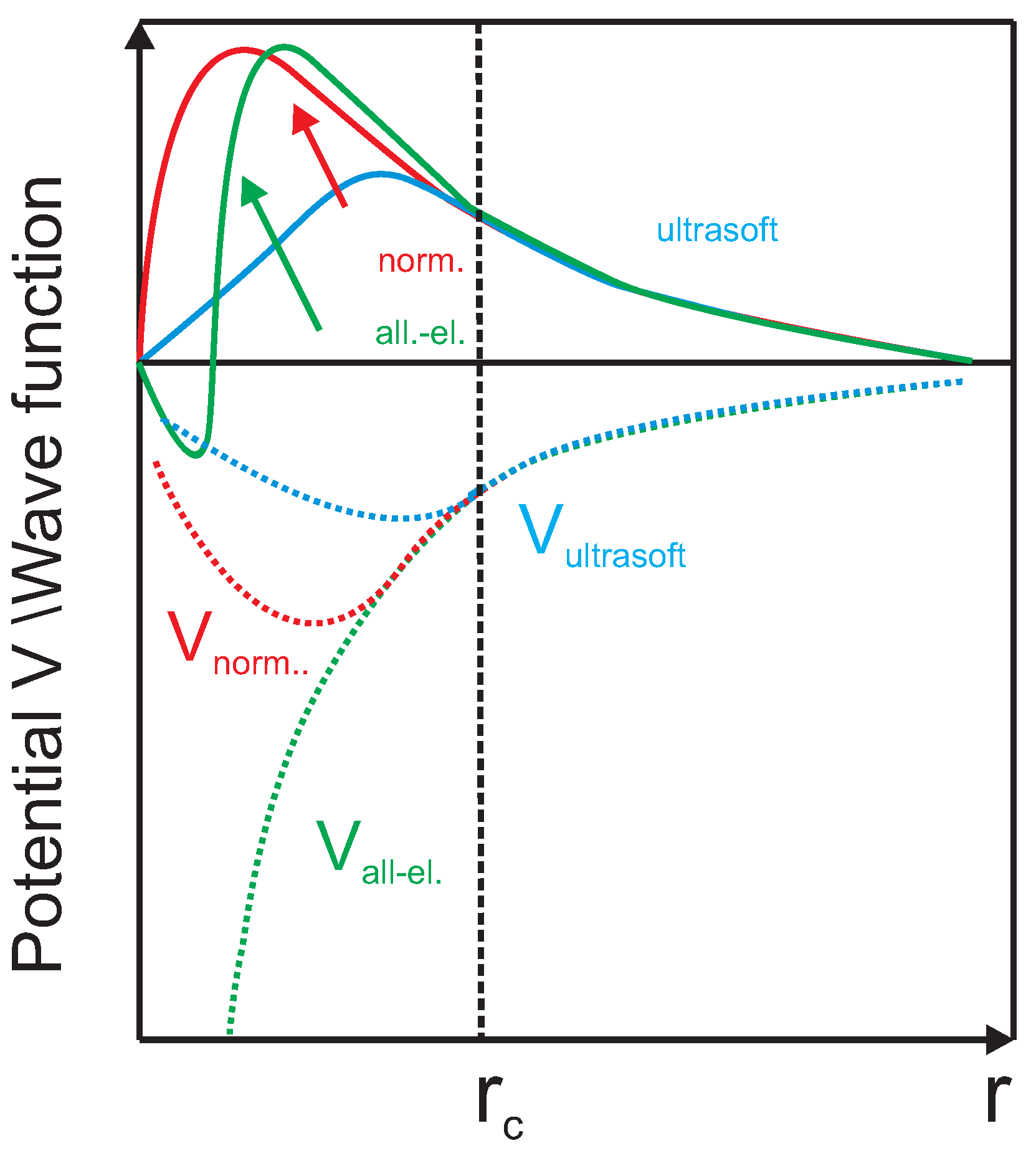
Appendix B.1.3. Pseudo Potential
- The eigenvalues of the pseudo potential must agree with the ones of the real potential.
- Above the cutoff radius , the wave functions of the pseudo potential must be equal to the true total electron wave function.
- The total charge within corresponds to the charge of the real total wave function.
- At and , the derivative of the pseudo-potential wave functions must agree with the real derivatives.
Appendix B.1.4. Band Structure
Appendix B.1.5. Dielectric Function
Appendix B.2. Normal Mode Analysis
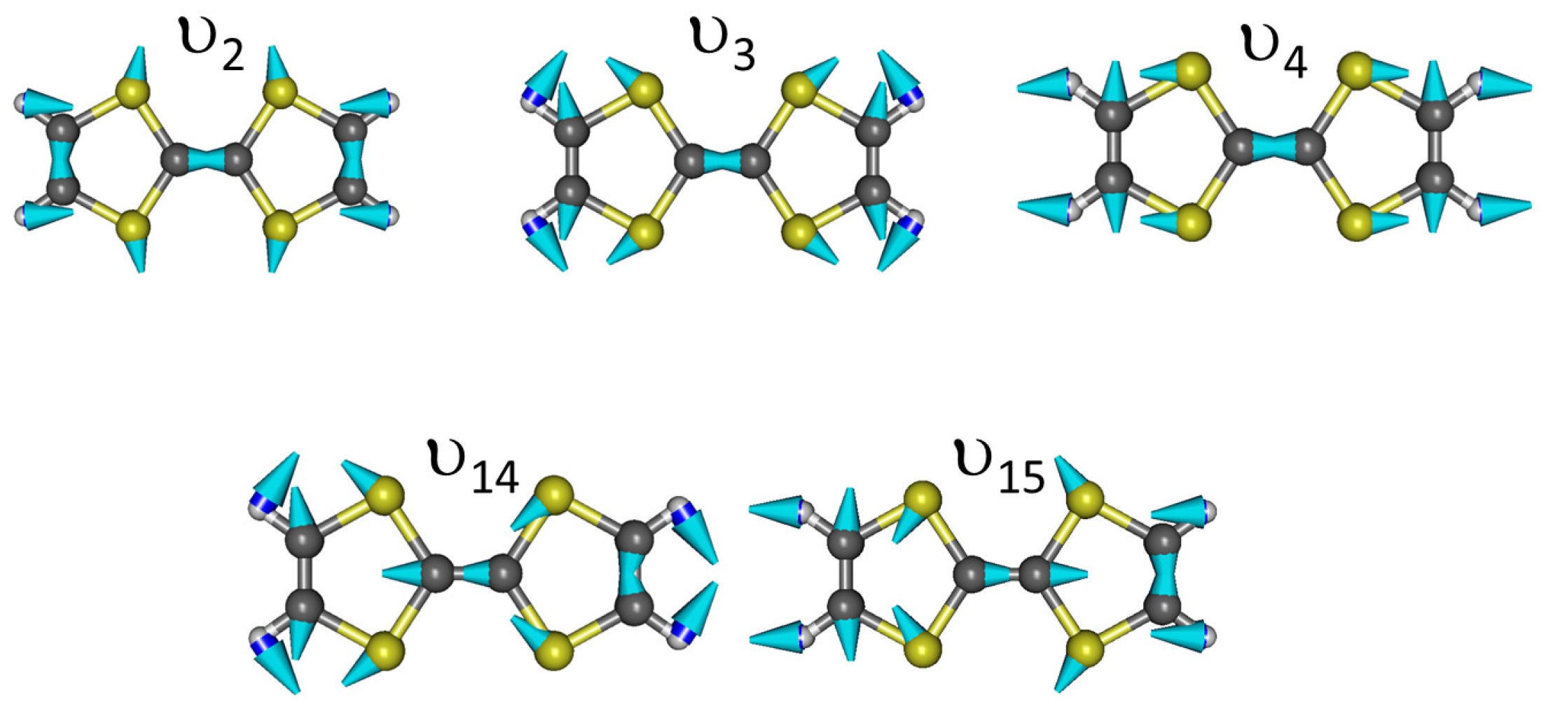
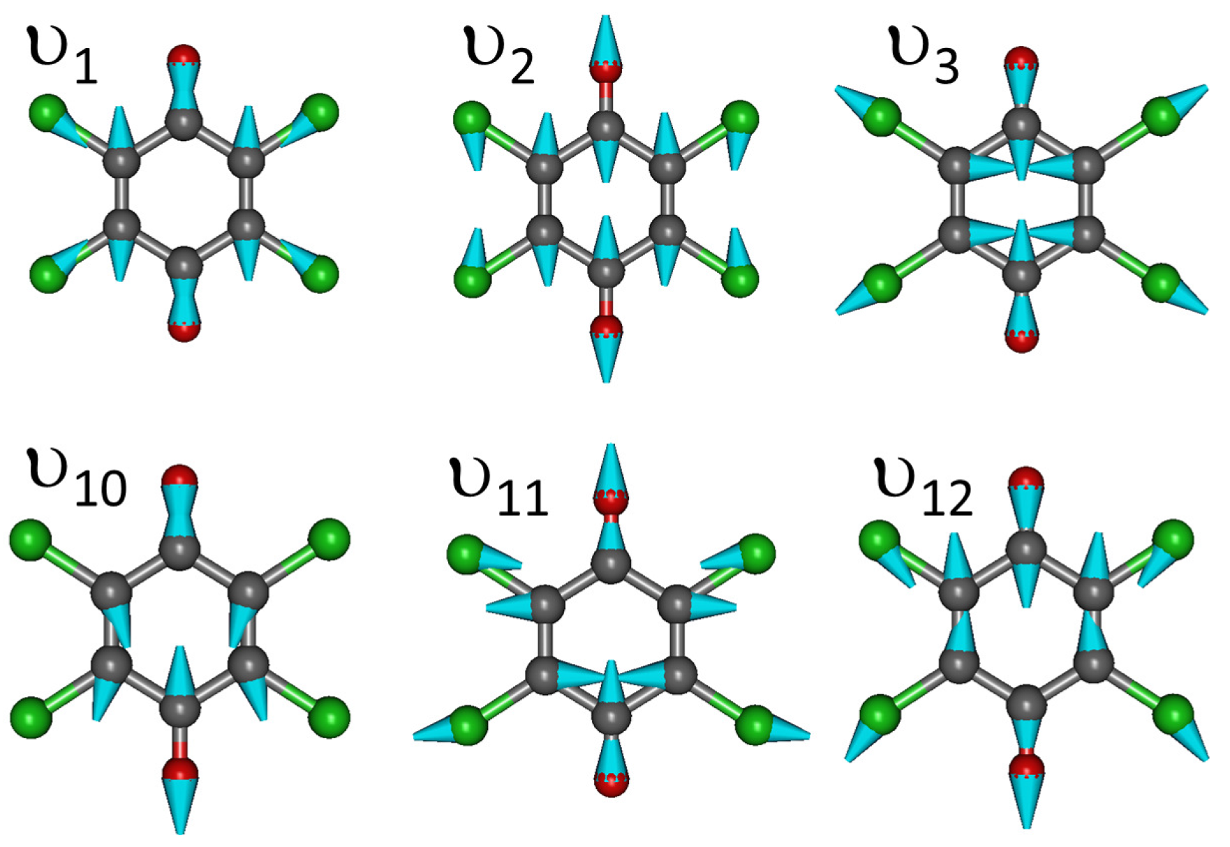
Appendix C. Vibrational Features of TTF and CA Molecules

| Label | Symmetry | CA0 | CA− | |||||
|---|---|---|---|---|---|---|---|---|
| Int. | Int. | |||||||
| a | 1754.1 | 1696.22 | - | 1548.51 | 1497.41 | - | −199 | |
| 1630.2 | 1576.24 | - | 1608.16 | 1555.09 | - | −21 | ||
| 970.94 | 990.07 | - | 982.53 | 1002 | - | 11.82 | ||
| 486.36 | 495.94 | - | 496.35 | 506.13 | - | 10.18 | ||
| 317.71 | 323.97 | - | 320.91 | 327.23 | - | 3.26 | ||
| 200.04 | 203.98 | - | 201.04 | 205 | - | 1.02 | ||
| b | 322.03 | 328.37 | - | 328.8 | 335.3 | - | 6.92 | |
| b | 801.56 | 817.35 | - | 771.93 | 787.13 | - | −29.93 | |
| 441.79 | 450.49 | - | 390.53 | 398.22 | - | −52.27 | ||
| 96.76 | 98.66 | - | 120.16 | 119.02 | - | 21.5 | ||
| b | 1215.35 | 1175.25 | - | 1301.89 | 1258.92 | - | 83.68 | |
| 829 | 845.33 | - | 807.37 | 823.28 | - | −22.06 | ||
| 733.82 | 748.28 | - | 724.12 | 738.4 | - | −10 | ||
| 337.27 | 343.92 | - | 325.54 | 331.96 | - | −12 | ||
| 263.81 | 269 | - | 275.46 | 281 | - | 11.88 | ||
| a | 573.15 | 584.44 | - | 559.45 | 570.47 | - | -13.96 | |
| 69.76 | 71.13 | - | 75.07 | 76.54 | - | 5.36 | ||
| b | 1757 | 1699 | 349.46 | 1565.35 | 1513.7 | 288.1 | −185.31 | |
| 1086.54 | 1050.68 | 415.77 | 1117.9 | 1081 | 203.72 | 30.32 | ||
| 899.07 | 916.78 | 25.31 | 892.53 | 910.12 | 159.74 | −6.67 | ||
| 460.13 | 469.2 | 5.27 | 436.92 | 445.53 | 0.66 | −23.66 | ||
| 205.26 | 209.3 | 0.03 | 205.46 | 209.51 | 1.44 | 0.21 | ||
| b | 1590.76 | 1538.26 | 254.54 | 1465 | 1416.57 | 0.27 | −121.7 | |
| 1202.63 | 1162.94 | 120.02 | 1099.8 | 1063.5 | 97.81 | −99.44 | ||
| 723.56 | 737.81 | 206.15 | 686.72 | 700.25 | 155.1 | −37.56 | ||
| 380.92 | 388.42 | 3.11 | 360.35 | 367.45 | 0.16 | −20.97 | ||
| 214.24 | 218.46 | 0.23 | 213.82 | 218.04 | 0.73 | −0.43 | ||
| b | 756.16 | 771.05 | 27.3 | 732.12 | 746.54 | 17.92 | −24.51 | |
| 199.7 | 203.62 | 2.88 | 201.47 | 205.44 | 2.76 | 1.82 | ||
| 69 | 70.33 | 1.68 | 86.8 | 88.5 | 3.12 | 18.17 | ||
| Label | Symmetry | TTF0 | TTF+ | |||||
|---|---|---|---|---|---|---|---|---|
| Int. | Int. | |||||||
| a | 3226.47 | 3120 | - | 3236.63 | 3129.82 | - | 9.83 | |
| 1621.92 | 1568.39 | - | 1551.15 | 1499.96 | - | −68.43 | ||
| 1.576 | 1524.41 | - | 1427.75 | 1380.63 | - | −143.78 | ||
| 1.125 | 1088 | - | 1130 | 1092.71 | - | 4.72 | ||
| 722.50 | 736.73 | - | 737.72 | 752.25 | - | 15.52 | ||
| 466.1 | 475.28 | - | 501.95 | 511.84 | - | 36.56 | ||
| 248.6 | 253.5 | - | 262.21 | 267.38 | - | 13.88 | ||
| b | 849 | 865.71 | - | 875.55 | 892.8 | - | 27.1 | |
| 419.08 | 427.34 | - | 435.66 | 444.24 | - | 16.91 | ||
| b | 632.63 | 645.09 | - | 688.56 | 702.13 | - | 57.03 | |
| 498.9 | 508.73 | - | 513.54 | 523.65 | - | 14.92 | ||
| 93.78 | 95.63 | - | 154.6 | 157.6 | - | 61.96 | ||
| b | 3206 | 3100.2 | - | 3220.42 | 3114.15 | - | 14 | |
| 1289.96 | 1247.4 | - | 1298.58 | 1255.72 | - | 8.34 | ||
| 967.9 | 986.97 | - | 1021.58 | 987.87 | - | 0.9 | ||
| 796.98 | 812.68 | - | 824.12 | 840.36 | - | 27.68 | ||
| 612.32 | 624.38 | - | 627.6 | 639.96 | 15.56 | |||
| 305.94 | 311.97 | - | 301.15 | 307.08 | - | −4.88 | ||
| a | 848.96 | 865.68 | - | 873.54 | 890.74 | - | 25.06 | |
| 415.72 | 423.91 | - | 424.94 | 433.31 | - | 9.40 | ||
| 92.4 | 94.22 | - | 65.36 | 66.64 | - | −27.57 | ||
| b | 3226.5 | 3120.03 | 0.5 | 3236.64 | 3129.83 | 28.57 | 9.8 | |
| 1598.57 | 1545.82 | 23.07 | 1532 | 1481.43 | 111.48 | −64.38 | ||
| 1124.65 | 1087.54 | 3.15 | 1130.92 | 1094 | 0.12 | 6.06 | ||
| 764.21 | 779.27 | 26.39 | 812 | 828 | 36.55 | 48.72 | ||
| 720.14 | 734.33 | 9.13 | 726.8 | 741.15 | 7.63 | 6.82 | ||
| 434.26 | 442.82 | 20.44 | 468.17 | 477.4 | 14.72 | 34.58 | ||
| b | 3206.9 | 3101.04 | 4.1 | 3220.6 | 3114.31 | 30.46 | 13.27 | |
| 1287.6 | 1245.11 | 0.02 | 1294.56 | 1251.84 | 8 | 6.73 | ||
| 823.4 | 839.62 | 7.7 | 868.33 | 885.44 | 7 | 45.82 | ||
| 786.91 | 802.41 | 56 | 823.81 | 840.04 | 26.51 | 37.63 | ||
| 621.37 | 633.61 | 2.76 | 636.68 | 649.27 | 1.19 | 15.61 | ||
| 114.31 | 116.56 | 0.58 | 123.45 | 125.88 | 0.28 | 9.32 | ||
| b | 633 | 645.46 | 160.31 | 690.13 | 703.73 | 164.7 | 58.27 | |
| 243.12 | 247.91 | 1.64 | 332.33 | 338.87 | 3.93 | 90.97 | ||
| 51.44 | 52.45 | 3.69 | 101.27 | 103.27 | 4.85 | 50.81 | ||
Appendix D. Heating Effect by Laser Radiation

References
- Torrance, J.B.; Mayerle, J.J.; Lee, V.Y.; Bechgaard, K. A new class of highly conducting organic materials: Charge-transfer salts of the tetrathiafulvalenes with the tetrahalo-p-benzoquinones. J. Am. Chem. Soc. 1979, 101, 4747–4748. [Google Scholar] [CrossRef]
- Le Cointe, M.; Lemée-Cailleau, M.H.; Cailleau, H.; Toudic, B.; Toupet, L.; Heger, G.; Moussa, F.; Schweiss, P.; Kraft, K.H.; Karl, N. Symmetry breaking and structural changes at the neutral-to-ionic transition in tetrathiafulvalene-p-chloranil. Phys. Rev. B 1995, 51, 3374–3386. [Google Scholar] [CrossRef]
- Mayerle, J.J.; Torrance, J.B.; Crowley, J.I. Mixed-stack complexes of tetrathiafulvalene. The structures of the charge-transfer complexes of TTF with chloranil and fluoranil. Acta Cryst. B 1979, 35, 2988–2995. [Google Scholar] [CrossRef]
- Girlando, A.; Marzola, F.; Pecile, C.; Torrance, J.B. Vibrational spectroscopy of mixed stack organic semiconductors: Neutral and ionic phases of tetrathiafulvalene-chloranil (TTF-CA) charge transfer complex. J. Chem. Phys. 1983, 79, 1075–1085. [Google Scholar] [CrossRef]
- Jacobsen, C.S.; Torrance, J.B. Behavior of charge-transfer absorption upon passing through the neutral-ionic phase transition. J. Chem. Phys. 1983, 78, 112–115. [Google Scholar] [CrossRef] [Green Version]
- Le Cointe-Buron, M.; Lemée-Cailleau, M.H.; Cailleau, H.; Luty, T. Condensation of Self–Trapped Charge–Transfer Excitations and Interplay between Quantum and Thermal Effects at the Neutral–to–Ionic Transition. J. Low Temp. Phys. 1998, 111, 677–691. [Google Scholar] [CrossRef]
- Cointe, M.L.; Lemée-Cailleau, M.; Cailleau, H.; Toudic, B. Structural aspects of the neutral-to-ionic transition in mixed-stack charge-transfer complexes. J. Mol. Struct. 1996, 374, 147–153. [Google Scholar]
- Girlando, A.; Bozio, R.; Pecile, C.; Torrance, J.B. Discovery of vibronic effects in the Raman spectra of mixed-stack charge-transfer crystals. Phys. Rev. B 1982, 26, 2306–2309. [Google Scholar] [CrossRef]
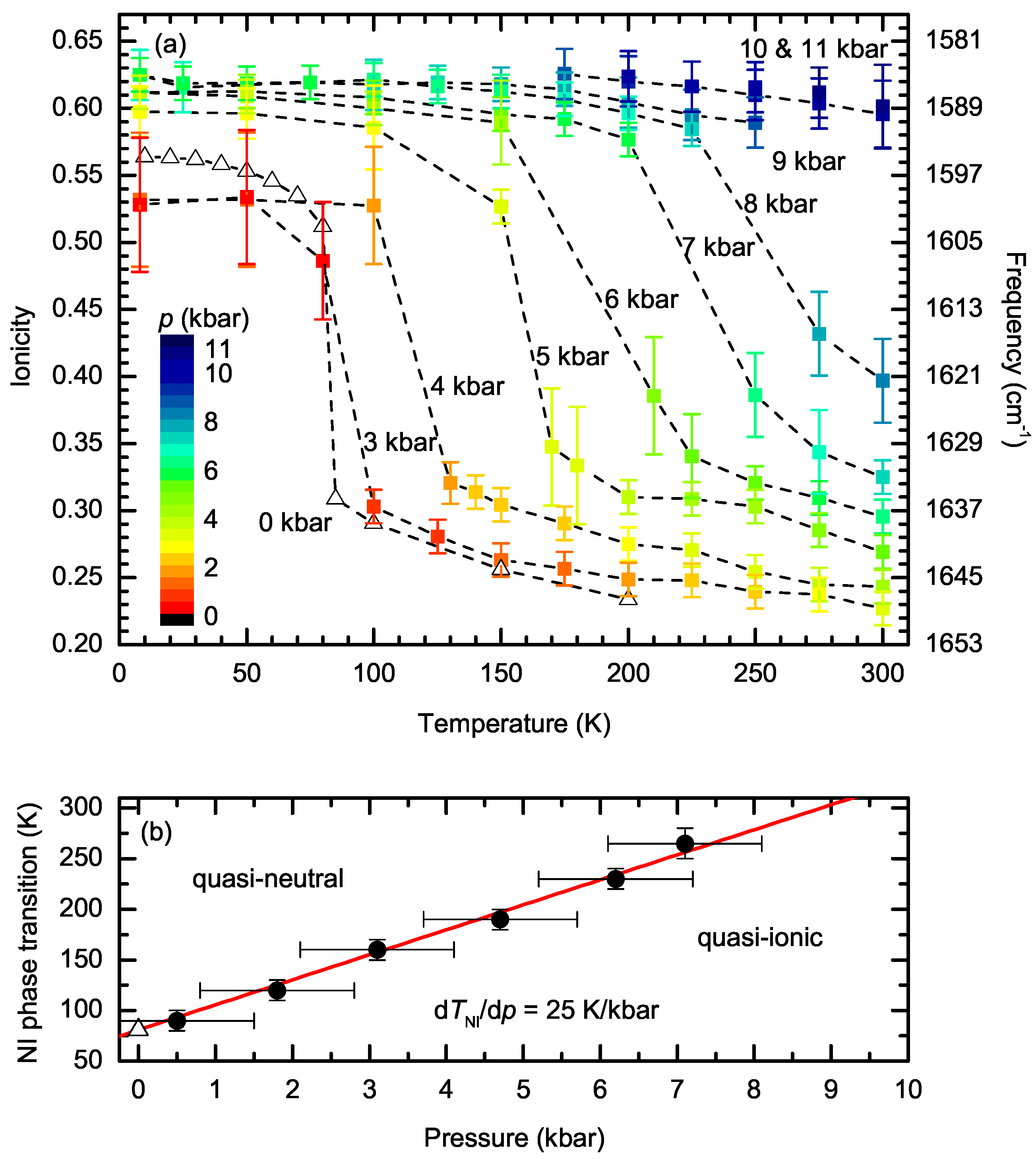
- Okamoto, H.; Mitani, T.; Tokura, Y.; Koshihara, S.; Komatsu, T.; Iwasa, Y.; Koda, T.; Saito, G. Anomalous dielectric response in tetrathiafulvalene-p-chloranil as observed in temperature- and pressure-induced neutral-to-ionic phase transition. Phys. Rev. B 1991, 43, 8224–8232. [Google Scholar] [CrossRef]
- Ayache, C.; Torrance, J. Multiple specific heat anomalies at the neutral-ionic phase transition in TTF-chloranil. Solid State Commun. 1983, 47, 789–793. [Google Scholar] [CrossRef]
- Mitani, T.; Kaneko, Y.; Tanuma, S.; Tokura, Y.; Koda, T.; Saito, G. Electric conductivity and phase diagram of a mixed-stack charge-transfer crystal: Tetrathiafulvalene-p-chloranil. Phys. Rev. B 1987, 35, 427–429. [Google Scholar] [CrossRef]
- Tokura, Y.; Okamoto, H.; Koda, T.; Mitani, T.; Saito, G. Nonlinear electric transport and switching phenomenon in the mixed-stack charge-transfer crystal tetrathiafulvalene-p-chloranil. Phys. Rev. B 1988, 38, 2215–2218. [Google Scholar] [CrossRef]
- McConnell, H.M.; Hoffman, B.M.; Metzger, R.M. Charge Transfer in Molecular Crystals. Proc. Natl. Acad. Sci. USA 1965, 53, 46–50. [Google Scholar] [CrossRef] [PubMed]
- Torrance, J.B.; Vazquez, J.E.; Mayerle, J.J.; Lee, V.Y. Discovery of a Neutral-to-Ionic Phase Transition in Organic Materials. Phys. Rev. Lett. 1981, 46, 253–257. [Google Scholar] [CrossRef]
- Katan, C. First-Principles Study of the Structures and Vibrational Frequencies for Tetrathiafulvalene TTF and TTF-d4 in Different Oxidation States. J. Phys. Chem. A 1999, 103, 1407–1413. [Google Scholar] [CrossRef]
- Lichtenberger, D.L.; Johnston, R.L.; Hinkelmann, K.; Suzuki, T.; Wudl, F. Relative electron donor strengths of tetrathiafulvene derivatives: Effects of chemical substitutions and the molecular environment from a combined photoelectron and electrochemical study. J. Am. Chem. Soc. 1990, 112, 3302–3307. [Google Scholar] [CrossRef]
- Sato, N.; Inokuchi, H.; Shirotani, I. Polarization energies of tetrathiafulvalene derivatives. Chem. Phys. 1981, 60, 327–333. [Google Scholar] [CrossRef]
- Batsanov, A.S.; Bryce, M.R.; Heaton, J.N.; Moore, A.J.; Skabara, P.J.; Howard, J.A.K.; Orti, E.; Viruela, P.M.; Viruela, R. New functionalized tetrathiafulvalenes: X-ray crystal structures and physico-chemical properties of TTF-C(O)NMe2 and TTF-C(O)-O-C4H9: A joint experimental and theoretical study. J. Mater. Chem. 1995, 5, 1689–1696. [Google Scholar] [CrossRef]
- Cooper, C.D.; Frey, W.F.; Compton, R.N. Negative ion properties of fluoranil, chloranil, and bromanil: Electron affinities. J. Chem. Phys. 1978, 69, 2367–2374. [Google Scholar] [CrossRef]
- Tanaka, S.; Aoki, S.; Nakayama, T.; Egusa, S. Effects of electrostatic field on the phase properties of mixed-stack organic charge-transfer compounds. Phys. Rev. B 1995, 52, 1549–1565. [Google Scholar] [CrossRef]
- Dengl, A.; Beyer, R.; Peterseim, T.; Ivek, T.; Untereiner, G.; Dressel, M. Evolution of ferroelectricity in tetrathiafulvalene-p-chloranil as a function of pressure and temperature. J. Chem. Phys. 2014, 140, 244511. [Google Scholar] [CrossRef] [PubMed]
- Nagaosa, N.; Takimoto, J.I. Theory of Neutral-Ionic Transition in Organic Crystals. I. Monte Carlo Simulation of Modified Hubbard Model. J. Phys. Soc. Jpn. 1986, 55, 2735–2744. [Google Scholar] [CrossRef]
- Nagaosa, N.; Takimoto, J.I. Theory of Neutral-Ionic Transition in Organic Crystals. II. Effect of the Intersite Coulomb Interaction. J. Phys. Soc. Jpn. 1986, 55, 2745–2753. [Google Scholar] [CrossRef]
- Soos, Z.G.; Painelli, A. Metastable domains and potential energy surfaces in organic charge-transfer salts with neutral-ionic phase transitions. Phys. Rev. B 2007, 75, 155119. [Google Scholar] [CrossRef]
- Mitani, T.; Tokura, Y.; Kaneko, Y.; Takaoka, K.; Koda, T.; Saito, G. Phase transition of the mixed-stack charge-transfer TTF-p-chloranil single crystals. Synth. Met. 1987, 19, 515–520. [Google Scholar] [CrossRef]
- Kambe, T.; Nogami, Y.; Oshima, K.; Takahashi, Y.; Sakai, H.; Koshihara, S. Soliton dynamics in TTF-CA. Synth. Met. 1999, 103, 1824. [Google Scholar] [CrossRef]
- Mitani, T.; Saito, G.; Tokura, Y.; Koda, T. Soliton Formation at the Neutral-to-Ionic Phase Transition in the Mixed-Stack Charge-Transfer Crystal Tetrathiafulvalene-p-Chloranil. Phys. Rev. Lett. 1984, 53, 842–845. [Google Scholar] [CrossRef]
- Takaoka, K.; Kaneko, Y.; Okamoto, H.; Tokura, Y.; Koda, T.; Mitani, T.; Saito, G. Infrared molecular-vibration spectra of tetrathiafulvalene-chloranil crystal at low temperature and high pressure. Phys. Rev. B 1987, 36, 3884–3887. [Google Scholar] [CrossRef]
- Okamoto, H.; Koda, T.; Tokura, Y.; Mitani, T.; Saito, G. Pressure-induced neutral-to-ionic phase transition in organic charge-transfer crystals of tetrathiafulvalene-p-benzoquinone derivatives. Phys. Rev. B 1989, 39, 10693–10701. [Google Scholar] [CrossRef]
- Kaneko, Y.; Tanuma, S.; Tokura, Y.; Koda, T.; Mitani, T.; Saito, G. Optical reflectivity spectra of the mixed-stack organic charge-transfer crystal tetrathiafulvalene-p-chloranil under hydrostatic pressure. Phys. Rev. B 1987, 35, 8024–8029. [Google Scholar] [CrossRef]
- Tokura, Y.; Okamoto, H.; Koda, T.; Mitani, T. Pressure-induced neutral-to-ionic phase transition in TTF-p-chloranil studied by infrared vibrational spectrocopy. Solid State Commun. 1986, 57, 607–610. [Google Scholar] [CrossRef]
- Girlando, A.; Painelli, A. Regular-dimerized stack and neutral-ionic interfaces in mixed-stack organic charge-transfer crystals. Phys. Rev. B 1986, 34, 2131–2139. [Google Scholar] [CrossRef]
- Masino, M.; Girlando, A.; Brillante, A. Intermediate regime in pressure-induced neutral-ionic transition in tetrathiafulvalene-chloranil. Phys. Rev. B 2007, 76, 064114. [Google Scholar] [CrossRef]
- Lemée-Cailleau, M.H.; Le Cointe, M.; Cailleau, H.; Luty, T.; Moussa, F.; Roos, J.; Brinkmann, D.; Toudic, B.; Ayache, C.; Karl, N. Thermodynamics of the Neutral-to-Ionic Transition as Condensation and Crystallization of Charge-Transfer Excitations. Phys. Rev. Lett. 1997, 79, 1690–1693. [Google Scholar] [CrossRef]
- Luty, T.; Cailleau, H.; Koshihara, S.; Collet, E.; Takesada, M.; Lemée-Cailleau, M.H.; Cointe, M.B.L.; Nagaosa, N.; Tokura, Y.; Zienkiewicz, E.; et al. Static and dynamic order of cooperative multi-electron transfer. Europhys. Lett. 2002, 59, 619–625. [Google Scholar] [CrossRef]
- Engler, E.M.; Patel, V.V.; Andersen, J.R.; Tomkiewicz, Y.; Craven, R.A.; Scott, B.A.; Etemad, S. Synthetic Approaches to the Study of Organic Metals. Ann. N. Y. Acad. Sci. 1978, 313, 343–354. [Google Scholar] [CrossRef]
- Demaniets, L.N. Organic Crystals; Germanates; Semiconductors; Springer: Berlin/Heidelberg, Germany; New York, NY, USA, 1980. [Google Scholar]
- Schwoerer, M.; Wolf, H. Organic Molecular Solids; Wiley-VCH: Weinheim, Germany, 2007. [Google Scholar]
- Williams, J.M.; Ferraro, J.R.; Thorn, R.J.; Carlson, K.D.; Geiser, U.; Wang, H.H.; Kini, A.M.; Whangbo, M.H. Organic Superconductors (Including Fullerenes: Synthesis, Structure, Properties, and Theory); Prentice Hall: Englewood Cliffs, NJ, USA, 1992. [Google Scholar]
- Yamada, J.; Sugimoto, T. (Eds.) TTF Chemistry: Fundamentals and Applications of Tetrathiafulvalene; Springer: Berlin/Heidelberg, Germany; New York, NY, USA, 2004.
- Lebed, A. (Ed.) The Physics of Organic Superconductors and Conductors; Springer Series in Materials Science; Springe: Berlin, Germany, 2008; Volume 110.
- Lin, C.Y.; George, M.W.; Gill, P.M.W. EDF2: A Density Functional for Predicting Molecular Vibrational Frequencies. Aust. J. Chem. 2004, 57, 365–370. [Google Scholar] [CrossRef]
- Wavefunction, Inc. Spartan’14 for Windows, Maxintosh and Linux; Wavefunction, Inc.: Irvine, CA, USA, 2014. [Google Scholar]
- Merrick, J.P.; Moran, D.; Radom, L. An Evaluation of Harmonic Vibrational Frequency Scale Factors. J. Phys. Chem. A 2007, 111, 11683–11700. [Google Scholar] [CrossRef] [PubMed]
- Ranzieri, P.; Masino, M.; Girlando, A. Charge-Sensitive Vibrations in p-Chloranil: The Strange Case of the C=C Antisymmetric Stretching. J. Phys. Chem. B 2007, 111, 12844–12848. [Google Scholar] [CrossRef] [PubMed]
- Liu, R.; Zhou, X.; Kasmai, H. Toward understanding the vibrational spectra of BEDT-TTF, a scaled density functional force field approach. Spectrochim. Acta A 1997, 53, 1241–1256. [Google Scholar] [CrossRef]
- Bozio, R.; Zanon, I.; Girlando, A.; Pecile, C. Vibrational spectroscopy of molecular constituents of one-dimensional organic conductors. Tetrathiofulvalene (TTF), TTF+, and (TTF+)2 dimer. J. Chem. Phys. 1979, 71, 2282–2293. [Google Scholar] [CrossRef]
- Dressel, M.; Dumm, M.; Knoblauch, T.; Masino, M. Comprehensive Optical Investigations of Charge Order in Organic Chain Compounds (TMTTF)2X. Crystals 2012, 2, 528–578. [Google Scholar] [CrossRef]
- Girlando, A.; Zanon, I.; Bozio, R.; Pecile, C. Raman and infrared frequency shifts proceeding from ionization of perhalo-p-benzoquinones to radical anions. J. Chem. Phys. 1978, 68, 22–31. [Google Scholar] [CrossRef]
- Garcia, P.; Dahaoui, S.; Katan, C.; Souhassou, M.; Lecomte, C. On the accurate estimation of intermolecular interactions and charge transfer: The case of TTF-CA. Faraday Discuss. 2007, 135, 217–235. [Google Scholar] [CrossRef] [PubMed]
- Giannozzi, P.; Baroni, S.; Bonini, N.; Calandra, M.; Car, R.; Cavazzoni, C.; Ceresoli, D.; Chiarotti, G.L.; Cococcioni, M.; Dabo, I.; et al. QUANTUM ESPRESSO: A modular and open-source software project for quantum simulations of materials. J. Phys. Condens. Matter 2009, 21, 395502. [Google Scholar] [CrossRef] [PubMed]
- Perdew, J.P.; Burke, K.; Ernzerhof, M. Generalized Gradient Approximation Made Simple. Phys. Rev. Lett. 1996, 77, 3865–3868. [Google Scholar] [CrossRef] [PubMed]
- Vanderbilt, D. Soft self-consistent pseudopotentials in a generalized eigenvalue formalism. Phys. Rev. B 1990, 41, 7892–7895. [Google Scholar] [CrossRef]
- Monkhorst, H.J.; Pack, J.D. Special points for Brillouin-zone integrations. Phys. Rev. B 1976, 13, 5188–5192. [Google Scholar] [CrossRef]
- Yu, P.Y.; Cardona, M. Fundamentals of Semiconductors: Physics and Materials Properties, 4th ed.; Graduate Texts in Physics; Springer: Berlin, Germany; London, UK, 2010. [Google Scholar]
- Oison, V.; Katan, C.; Koenig, C. Intramolecular Electronic Redistribution Coupled to Hydrogen Bonding: An Important Mechanism for the “Neutral-to-Ionic” Transition. J. Phys. Chem. A 2001, 105, 4300–4307. [Google Scholar] [CrossRef]
- Dressel, M.; Drichko, N. Optical Properties of Two-Dimensional Organic Conductors: Signatures of Charge Ordering and Correlation Effects. Chem. Rev. 2004, 104, 5689–5716. [Google Scholar] [CrossRef] [PubMed]
- Tomic, S.; Dressel, M. Ferroelectricity in molecular solids: A review of electrodynamic properties. Rep. Prog. Phys. 2015, 78, 096501. [Google Scholar] [CrossRef] [PubMed]
- Girlando, A.; Pecile, C.; Brillante, A.; Syassen, K. High pressure optical studies of neutral-ionic phase transitions in organic charge-transfer crystals. Synth. Met. 1987, 19, 503–508. [Google Scholar] [CrossRef]
- Cointe, M.B.L.; Lemée-Cailleau, M.H.; Cailleau, H.; Toudic, B.; Moréac, A.; Moussa, F.; Ayache, C.; Karl, N. Thermal hysteresis phenomena and mesoscopic phase coexistence around the neutral-ionic phase transition in TTF-CA and TMB-TCNQ. Phys. Rev. B 2003, 68, 064103. [Google Scholar] [CrossRef]
- Ivek, T.; Korin-Hamzić, B.; Milat, O.; Tomić, S.; Clauss, C.; Drichko, N.; Schweitzer, D.; Dressel, M. Collective Excitations in the Charge-Ordered Phase of α-(BEDT-TTF)2I3. Phys. Rev. Lett. 2010, 104, 206406. [Google Scholar] [CrossRef] [PubMed]
- Ivek, T.; Korin-Hamzić, B.; Milat, O.; Tomić, S.; Clauss, C.; Drichko, N.; Schweitzer, D.; Dressel, M. Electrodynamic Response of the Charge Ordering Phase: Dielectric and Optical Studies of α-(BEDT-TTF)2I3. Phys. Rev. B 2011, 83, 165128. [Google Scholar] [CrossRef]
- Alemany, P.; Pouget, J.P.; Canadell, E. Essential Role of Anions in the Charge Ordering Transition in α-(BEDT-TTF)2I3. Phys. Rev. B 2012, 85, 195118. [Google Scholar] [CrossRef]
- Beyer, R.; Dengl, A.; Peterseim, T.; Wackerow, S.; Ivek, T.; Pronin, A.; Schweitzer, D.; Dressel, M. Pressure-dependent optical investigations of α-(BEDT-TTF)2I3: Tuning charge order and narrow gap towards a Dirac semimetal. Phys. Rev. B 2016, 93, 195116. [Google Scholar] [CrossRef]
- Girlando, A.; Masino, M.; Painelli, A.; Drichko, N.; Dressel, M.; Brillante, A.; Della Valle, R.G.; Venuti, E. Direct evidence of overdamped Peierls-coupled modes in the temperature-induced phase transition in tetrathiafulvalene-chloranil. Phys. Rev. B 2008, 78, 045103. [Google Scholar] [CrossRef]
- Tadashi, S.; Kyuya, Y.; Haruo, K. Polarized Absorption Spectra of Single Crystals of Tetrathiafulvalenium Salts. Bull. Chem. Soc. Jpn. 1978, 51, 1041–1046. [Google Scholar]
- Masashi, T. Electronic States of the Crystals of TCNE Complexes with Hexamethylbenzene, Acenaphthene, and Dibenzofuran. Bull. Chem. Soc. Jpn. 1977, 50, 2881–2884. [Google Scholar]
- Masino, M.; Girlando, A.; Soos, Z.G. Evidence for a soft mode in the temperature induced neutral-ionic transition of TTF-CA. Chem. Phys. Lett. 2003, 369, 428–433. [Google Scholar] [CrossRef]
- Koshihara, S.; Tokura, Y.; Mitani, T.; Saito, G.; Koda, T. Photoinduced valence instability in the organic molecular compound tetrathiafulvalene-p-chloranil (TTF-CA). Phys. Rev. B 1990, 42, 6853–6856. [Google Scholar] [CrossRef]
- Koshihara, S.; Takahashi, Y.; Sakai, H.; Tokura, Y.; Luty, T. Photoinduced Cooperative Charge Transfer in Low-Dimensional Organic Crystals. J. Phys. Chem. B 1999, 103, 2592–2600. [Google Scholar] [CrossRef]
- Huai, P.; Zheng, H.; Nasu, K. Theory for Photoinduced Ionic-Neutral Structural Phase Transition in Quasi One-Dimensional Organic Molecular Crystal TTF-CA. J. Phys. Soc. Jpn. 2000, 69, 1788–1800. [Google Scholar] [CrossRef]
- Collet, E.; Lemée-Cailleau, M.H.; Cointe, M.B.L.; Cailleau, H.; Ravy, S.; Luty, T.; Bérar, J.F.; Czarnecki, P.; Karl, N. Direct evidence of lattice-relaxed charge transfer exciton strings. Europhys. Lett. 2002, 57, 67–73. [Google Scholar] [CrossRef]
- Iwai, S.; Tanaka, S.; Fujinuma, K.; Kishida, H.; Okamoto, H.; Tokura, Y. Ultrafast Optical Switching from an Ionic to a Neutral State in Tetrathiafulvalene-p-Chloranil (TTF-CA) Observed in Femtosecond Reflection Spectroscopy. Phys. Rev. Lett. 2002, 88, 057402. [Google Scholar] [CrossRef] [PubMed]
- Nasu, K. (Ed.) Photoinduced Phase Transition; Word Scientific: Singapore, 2004.
- Tanimura, K. Femtosecond time-resolved reflection spectroscopy of photoinduced ionic-neutral phase transition in TTF-CA crystals. Phys. Rev. B 2004, 70, 144112. [Google Scholar] [CrossRef]
- Okamoto, H.; Ishige, Y.; Tanaka, S.; Kishida, H.; Iwai, S.; Tokura, Y. Photoinduced phase transition in tetrathiafulvalene-p-chloranil observed in femtosecond reflection spectroscopy. Phys. Rev. B 2004, 70, 165202. [Google Scholar] [CrossRef]
- Guérin, L.; Collet, E.; Lemée-Cailleau, M.H.; Cointe, M.B.L.; Cailleau, H.; Plech, A.; Wulff, M.; Koshihara, S.Y.; Luty, T. Probing photoinduced phase transition in a charge-transfer molecular crystal by 100 picosecond X-ray diffraction. Chem. Phys. 2004, 299, 163–170. [Google Scholar] [CrossRef]
- Collet, E.; Cointe, M.B.L.; Cailleau, H. X-ray Diffraction Investigation of the Nature and the Mechanism of Photoinduced Phase Transition in Molecular Materials. J. Phys. Soc. Jpn. 2006, 75, 011002. [Google Scholar] [CrossRef]
- Tokura, Y. Photoinduced Phase Transition: A Tool for Generating a Hidden State of Matter. J. Phys. Soc. Jpn. 2006, 75, 011001. [Google Scholar] [CrossRef]
- Yonemitsu, K. Theory of Photoinduced Phase Transitions in Molecular Conductors: Interplay between Correlated Electrons, Lattice Phonons and Molecular Vibrations. Crystals 2012, 2, 56–77. [Google Scholar] [CrossRef]
- Iwai, S.; Okamoto, H. Ultrafast Phase Control in One-Dimensional Correlated Electron Systems. J. Phys. Soc. Jpn. 2006, 75, 011007. [Google Scholar] [CrossRef]
- Matsubara, Y.; Okimoto, Y.; Yoshida, T.; Ishikawa, T.; Koshihara, S.Y.; Onda, K. Photoinduced Neutral-to-Ionic Phase Transition in Tetrathiafulvalene-p-chloranil Studied by Time-Resolved Vibrational Spectroscopy. J. Phys. Soc. Jpn. 2011, 80, 124711. [Google Scholar] [CrossRef]
- Peterseim, T.; Haremski, P.; Dressel, M. Random-walk annihilation process of photo-induced neutral-ionic domain walls in TTF-CA. Europhys. Lett. 2015, 109, 67003. [Google Scholar] [CrossRef]
- Peterseim, T.; Dressel, M. Molecular Dynamics at Electrical- and Optical-Driven Phase Transitions: Time-Resolved Infrared Studies Using Fourier-Transform Spectrometers. arXiv, 2016; 10.1007/s10762-016-0294-5. [Google Scholar]
- Suzuki, T.; Sakamaki, T.; Tanimura, K.; Koshihara, S.; Tokura, Y. Ionic-to-neutral phase transformation induced by photoexcitation of the charge-transfer band in tetrathiafulvalene-p-chloranil crystals. Phys. Rev. B 1999, 60, 6191–6193. [Google Scholar] [CrossRef]
- Tanimura, K.; Koshihara, S. Photo-induced ionic-to-neutral phase transition in tetrathiafulvalen-p-chloranil crystals. Phase Transit. 2001, 74, 21–34. [Google Scholar] [CrossRef]
- Iwai, S.; Ishige, Y.; Tanaka, S.; Okimoto, Y.; Tokura, Y.; Okamoto, H. Coherent Control of Charge and Lattice Dynamics in a Photoinduced Neutral-to-Ionic Transition of a Charge-Transfer Compound. Phys. Rev. Lett. 2006, 96, 057403. [Google Scholar] [CrossRef] [PubMed]
- Tanimura, K.; Akimoto, I. Femtosecond time-resolved spectroscopy of photoinduced ionic-to-neutral phase transition in tetrathiafulvalen-p-chloranil crystals. J. Lumin. 2001, 94–95, 483–488. [Google Scholar] [CrossRef]
- Tokura, Y.; Koda, T.; Mitani, T.; Saito, G. Neutral-to-ionic transition in tetrathiafulvalene-p-chloranil as investigated by optical reflection spectra. Solid State Commun. 1982, 43, 757–760. [Google Scholar] [CrossRef]
- Hünig, S.; Kießlich, G.; Quast, H.; Scheutzow, D. Über zweistufige Redoxsysteme, X1 Tetrathio-äthylene und ihre höheren Oxidationsstufen. Justus Liebigs Ann. Chem. 1973, 1973, 310–323. [Google Scholar] [CrossRef]
- Wudl, F.; Kruger, A.A.; Kaplan, M.L.; Hutton, R.S. Unsymmetrical dimethyltetrathiafulvalene. J. Org. Chem. 1977, 42, 768–770. [Google Scholar] [CrossRef]
- Coffen, D.L.; Chambers, J.Q.; Williams, D.R.; Garrett, P.E.; Canfield, N.D. Tetrathioethylenes. J. Am. Chem. Soc. 1971, 93, 2258–2268. [Google Scholar] [CrossRef]
- Andre, J.; Weill, G. Optical spectrum of the chloranil radical anion. Mol. Phys. 1968, 15, 97–99. [Google Scholar] [CrossRef]
- Nobuko, S.; Ichimin, S.; Shigeru, M. The Effect of Pressure on the Electronic Absorption Spectra of Alkali Metal Cation-Chloranil and -Bromanil Anion Radical Salts, and the Dimerization of the Chloranil Anion Radical in Solution. Bull. Chem. Soc. Jpn. 1971, 44, 675–679. [Google Scholar]
- Bieber, A.; Andre, J. Some electronic properties of TMPD, CA and TCNQ molecules and their mono- and diions. Chem. Phys. 1974, 5, 166–182. [Google Scholar] [CrossRef]
- Pope, M.; Swenberg, C.E. Electronic Processes in Organic Crystals and Polymers, 2nd ed.; Monographs on the Physics and Chemistry of Materials; Oxford University Press: New York, NY, USA, 1999; Volume 56. [Google Scholar]
- Hoshino, M.; Nozawa, S.; Sato, T.; Tomita, A.; Adachi, S.I.; Koshihara, S.Y. Time-resolved X-ray crystal structure analysis for elucidating the hidden ‘over-neutralized’ phase of TTF-CA. RSC Adv. 2013, 3, 16313–16317. [Google Scholar] [CrossRef]
- Dressel, M.; Grüner, G. Electrodynamics of Solids; Cambridge University Press: Cambridge, UK, 2002. [Google Scholar]
- Nagahori, A.; Kubota, N.; Itoh, C. Time-resolved Fourier-transform infrared reflection study on photoinduced phase transition of tetrathiafulvalene-p-chloranil crystal. Eur. Phys. J. B 2013, 86, 109–142. [Google Scholar] [CrossRef]
- Djurek, D.; Jerome, D.; Bechgaard, K. Thermal transport properties of organic conductors: (TMTSF)2PF6 and (TMTSF)2ClO4. J. Phys. C Solid State Phys. 1984, 17, 4179–4192. [Google Scholar] [CrossRef]
- Bechtel, J.H. Heating of solid targets with laser pulses. J. Appl. Phys. 1975, 46, 1585–1593. [Google Scholar] [CrossRef]
- Salamon, M.B.; Bray, J.W.; DePasquali, G.; Craven, R.A.; Stucky, G.; Schultz, A. Thermal conductivity of tetrathiafulvalene-tetracyanoquinodimethane (TTF-TCNQ) near the metal-insulator transition. Phys. Rev. B 1975, 11, 619–622. [Google Scholar] [CrossRef]
- Matsukawa, M.; Hashimoto, K.; Yoshimoto, N.; Yoshizawa, M.; Kashiwaba, Y.; Noto, K. Thermal Conductivity in the ab-Plane of the Organic Conductor α-BEDT-TTF)2I3. J. Phys. Soc. Jpn. 1995, 64, 2233–2234. [Google Scholar] [CrossRef]
- Nasu, K. Relaxations of Excited States and Photo-Induced Structural Phase Transitions; Springer Series in Solid-State Sciences; Springer: Berlin/Heidelberg, Germany, 1997; Volume 124. [Google Scholar]
- Kuroda, N.; Wakabayashi, Y.; Nishida, M.; Wakabayashi, N.; Yamashita, M.; Matsushita, N. Decay Kinetics of Long-Lived Photogenerated Kinks in an MX Chain Compound. Phys. Rev. Lett. 1997, 79, 2510–2513. [Google Scholar] [CrossRef]
- Tabata, Y.; Kuroda, N. Decay Kinetics of Photoinduced Solitons on a One-Dimensional Lattice with Traps. J. Phys. Soc. Jpn. 2009, 78, 034704. [Google Scholar] [CrossRef] [Green Version]
- Koshihara, S.; Tokura, Y.; Sarukura, N.; Segawa, Y.; Koda, T.; Takeda, K. Nanosecond and picosecond dynamics of photo-induced phase-transition in low dimensional organic crystals. Synth. Met. 1995, 70, 1225–1226. [Google Scholar] [CrossRef]
- Bleier, H.; Roth, S.; Shen, Y.Q.; Schäfer-Siebert, D.; Leising, G. Photoconductivity in trans-polyacetylene: Transport and recombination of photogenerated charged excitations. Phys. Rev. B 1988, 38, 6031–6040. [Google Scholar] [CrossRef]
- Shank, C.V.; Yen, R.; Fork, R.L.; Orenstein, J.; Baker, G.L. Picosecond Dynamics of Photoexcited Gap States in Polyacetylene. Phys. Rev. Lett. 1982, 49, 1660–1663. [Google Scholar] [CrossRef]
- Privman, V. Nonequilibrium Statistical Mechanics in One Dimension; Cambridge University Press: Cambridge, UK; New York, NY, USA, 1997. [Google Scholar]
- Torney, D.C.; McConnell, H.M. Diffusion-limited reactions in one dimension. J. Phys. Chem. 1983, 87, 1941–1951. [Google Scholar] [CrossRef]
- Lushnikov, A. Binary reaction 1 + 1 → 0 in one dimension. Phys. Lett. A 1987, 120, 135–137. [Google Scholar] [CrossRef]
- Balding, D.; Clifford, P.; Green, N. Invasion processes and binary annihilation in one dimension. Phys. Lett. A 1988, 126, 481–483. [Google Scholar] [CrossRef]
- Sasaki, K.; Nakagawa, T. Exact Results for a Diffusion-Limited Pair Annihilation Process on a One-Dimensional Lattice. J. Phys. Soc. Jpn. 2000, 69, 1341–1351. [Google Scholar] [CrossRef]
- Ben Avraham, D. Computer simulation methods for diffusion-controlled reactions. J. Chem. Phys. 1988, 88, 941–948. [Google Scholar] [CrossRef]
- bwGRiD, Member of the German D-Grid Initiative, Funded by the Ministry for Education and Research (Bundesministerium für Bildung und Forschung) and the Ministry for Science, Research and Arts Baden-Wuerttemberg (Ministerium für Wissenschaft, Forschung und Kunst Baden-Württemberg). Available online: http://www.bw-grid.de (accessed on 4 January 2017).
- Fano, U. Effects of Configuration Interaction on Intensities and Phase Shifts. Phys. Rev. 1961, 124, 1866–1878. [Google Scholar] [CrossRef]
- Sedlmeier, K.; Elsässer, S.; Neubauer, D.; Beyer, R.; Wu, D.; Ivek, T.; Tomić, S.; Schlueter, J.A.; Dressel, M. Absence of charge order in the dimerized κ-phase BEDT-TTF salts. Phys. Rev. B 2012, 86, 245103. [Google Scholar] [CrossRef]
- Gordon, M.S.; Schmidt, M.W. Advances in electronic structure theory: {GAMESS} a decade later. In Theory and Applications of Computational Chemistry; Dykstra, C.E., Frenking, G., Kim, K.S., Scuseria, G.E., Eds.; Elsevier: Amsterdam, The Netherlands, 2005; Chapter 41; pp. 1167–1189. [Google Scholar]
- Schmidt, M.W.; Baldridge, K.K.; Boatz, J.A.; Elbert, S.T.; Gordon, M.S.; Jensen, J.H.; Koseki, S.; Matsunaga, N.; Nguyen, K.A.; Su, S.; et al. General atomic and molecular electronic structure system. J. Comput. Chem. 1993, 14, 1347–1363. [Google Scholar] [CrossRef]
- Perdew, J.P.; Schmidt, K. Jacob’s ladder of density functional approximations for the exchange-correlation energy. In Proceedings of the Conference on Density Functional Theory and Its Application To Materials, Antwep, Belgium, 8–10 June 2000.
- Becke, A.D. Density-functional exchange-energy approximation with correct asymptotic behavior. Phys. Rev. A 1988, 38, 3098–3100. [Google Scholar] [CrossRef]
- Lee, C.; Yang, W.; Parr, R.G. Development of the Colle-Salvetti correlation-energy formula into a functional of the electron density. Phys. Rev. B 1988, 37, 785–789. [Google Scholar] [CrossRef]
- Perdew, J.P.; Wang, Y. Accurate and simple analytic representation of the electron-gas correlation energy. Phys. Rev. B 1992, 45, 13244–13249. [Google Scholar] [CrossRef]
- Perdew, J.P.; Burke, K.; Ernzerhof, M. Generalized Gradient Approximation Made Simple. Phys. Rev. Lett. 1997, 78, 1396. [Google Scholar] [CrossRef]
- Becke, A.D. Density-functional thermochemistry. III. The role of exact exchange. J. Chem. Phys. 1993, 98, 5648–5652. [Google Scholar] [CrossRef]
- Becke, A.D. A new mixing of Hartree-Fock and local density-functionalq theories. J. Chem. Phys. 1993, 98, 1372–1377. [Google Scholar] [CrossRef]
- Stephens, P.J.; Devlin, F.J.; Chabalowski, C.F.; Frisch, M.J. Ab Initio Calculation of Vibrational Absorption and Circular Dichroism Spectra Using Density Functional Force Fields. J. Phys. Chem. 1994, 98, 11623–11627. [Google Scholar] [CrossRef]
- Adamo, C.; Barone, V. Toward reliable density functional methods without adjustable parameters: The PBE0 model. J. Chem. Phys. 1999, 110, 6158–6170. [Google Scholar] [CrossRef]
- Jensen, F. Introduction to Computational Chemistry, 2nd ed.; John Wiley & Sons: Chichester, UK; Hoboken, NJ, USA, 2007. [Google Scholar]
- Andersson, M.P.; Uvdal, P. New Scale Factors for Harmonic Vibrational Frequencies Using the B3LYP Density Functional Method with the Triple-ζ Basis Set 6-311+G(d,p). J. Phys. Chem. A 2005, 109, 2937–2941. [Google Scholar] [CrossRef] [PubMed]
- Carbonniere, P.; Lucca, T.; Pouchan, C.; Rega, N.; Barone, V. Vibrational computations beyond the harmonic approximation: Performances of the B3LYP density functional for semirigid molecules. J. Comput. Chem. 2005, 26, 384–388. [Google Scholar] [CrossRef] [PubMed]
- Gisslén, L.; Scholz, R. Crystallochromy of perylene pigments: Interference between Frenkel excitons and charge-transfer states. Phys. Rev. B 2009, 80, 115309. [Google Scholar] [CrossRef]
- Kokalj, A. XCrySDen—A new program for displaying crystalline structures and electron densities. J. Mol. Graph. Model. 1999, 17, 176–179. [Google Scholar] [CrossRef]
- Benassi, A. PWscf’s Epsilon.x User’s Manual. Available online: https://www.google.de/url?sa=t&rct=j&q=&esrc=s&source=web&cd=1&cad=rja&uact=8&ved=0ahUKEwjl5MbqqanRAhWFwBQKHWOMA_4QFggaMAA&url=https%3A%2F%2Fwww.researchgate.net%2Ffile.PostFileLoader.html%3Fid%3D567d1ab17eddd3eb328b4574%26assetKey%3DAS%253A310495943299072%25401451039409313&usg=AFQjCNGjbPOaQq47wPrCah_71TeU8DCUpw&sig2=D8sZeomhzyoi9HayKAfzDw (accessed on 30 November 2016).


| Parameter | TTF-CA (300 K) [3] | TTF-CA (40 K) [2] |
|---|---|---|
| a (Å) | 7.41 | 7.19 |
| b (Å) | 7.621 | 7.54 |
| c (Å) | 14.571 | 14.44 |
| α (°) | 90 | 90 |
| β (°) | 99.2 | 98.6 |
| γ (°) | 90 | 90 |
| V (Å) | 812.35 | 774.03 |
| Z | 2 | 2 |
| M (g·mol) | 900.74 | 900.74 |
| (g·cm) | 1.82 | 1.93 |
| Space group | P2/n | Pn |
| Label | Symmetry | CA0 | CA− | (cm) | (meV) | ||||
| Int. | Int. | ||||||||
| (cm) | (cm) | (cm) | (cm) | ||||||
| a | 1754.1 | 1696.22 | - | 1548.51 | 1497.41 | - | −199 | 67 | |
| 1630.2 | 1576.24 | - | 1608.16 | 1555.09 | - | −21 | 83 | ||
| 970.94 | 990.07 | - | 982.53 | 1002 | - | 12 | 95 | ||
| b | 1757 | 1699 | 349.46 | 1565.35 | 1513.7 | 288.1 | −185 | ||
| 1086.54 | 1050.68 | 415.77 | 1117.9 | 1081 | 203.72 | 30 | |||
| 899.07 | 916.78 | 25.31 | 892.53 | 910.12 | 159.74 | −7 | |||
| Label | Symmetry | TTF | TTF | ||||||
| Int. | Int. | ||||||||
| a | 1621.92 | 1568.39 | - | 1551.15 | 1499.96 | - | −68 | 16 | |
| 1.576 | 1524.41 | - | 1427.75 | 1380.63 | - | −144 | 115 | ||
| 1.125 | 1088 | - | 1130 | 1092.71 | - | 5 | 10 | ||
| b | 1598.57 | 1545.82 | 23.07 | 1532 | 1481.43 | 111.48 | −64 | ||
| 1124.65 | 1087.54 | 3.15 | 1130.92 | 1094 | 0.12 | 6 | |||
| Transition | Excitation Energy TTF [90] | Excitation Energy TTF [91,92] |
| in Acetonitril | in Hexan | |
| 1 | 17,300/2.14(0.27) | 22,200/2.76(0.02) |
| 2 | 20,300/2.51(weak) | 27,100/3.37(0.16) |
| 3 | 23,000/2.85(1.00) | 31,600/3.92(0.89) |
| 4 | 29,600/3.67(0.52) | 33,000/4.09(1.00) |
| Transition | Excitation Energy CA [93,94] | Excitation Energy CA [95] |
| 1 | 22,300/2.77(-) | 27,200/3.37(-) |
| 2 | 23,700/2.94(-) | 34,800/4.32(-) |
| 3 | 31,100/3.86(-) |
© 2017 by the authors; licensee MDPI, Basel, Switzerland. This article is an open access article distributed under the terms and conditions of the Creative Commons Attribution (CC-BY) license (http://creativecommons.org/licenses/by/4.0/).
Share and Cite
Dressel, M.; Peterseim, T. Infrared Investigations of the Neutral-Ionic Phase Transition in TTF-CA and Its Dynamics. Crystals 2017, 7, 17. https://doi.org/10.3390/cryst7010017
Dressel M, Peterseim T. Infrared Investigations of the Neutral-Ionic Phase Transition in TTF-CA and Its Dynamics. Crystals. 2017; 7(1):17. https://doi.org/10.3390/cryst7010017
Chicago/Turabian StyleDressel, Martin, and Tobias Peterseim. 2017. "Infrared Investigations of the Neutral-Ionic Phase Transition in TTF-CA and Its Dynamics" Crystals 7, no. 1: 17. https://doi.org/10.3390/cryst7010017