
The Physics of the Hume-Rothery Electron Concentration Rule

1
Nagoya Industrial Science Research Institute, 1-13 Yotsuya-dori, Chikusa-ku, Nagoya 464-0819, Japan
2
Department of Physics, Aichi University of Education, Kariya-shi, Aichi 448-8542, Japan
*
Author to whom correspondence should be addressed.
Crystals 2017, 7(1), 9; https://doi.org/10.3390/cryst7010009
Submission received: 17 October 2016
/
Revised: 10 December 2016
/
Accepted: 13 December 2016
/
Published: 6 January 2017
(This article belongs to the Special Issue Structure and Properties of Quasicrystals 2016)
Abstract
:For a long time we have shared the belief that the physics of the Hume-Rothery electron concentration rule can be deepened only through thorough investigation of the interference phenomenon of itinerant electrons with a particular set of lattice planes, regardless of whether d-states are involved near the Fermi level or not. For this purpose, we have developed the FLAPW-Fourier theory (Full potential Linearized Augmented Plane Wave), which is capable of determining the square of the Fermi diameter, , and the number of itinerant electrons per atom, e/a, as well as the set of lattice planes participating in the interference phenomenon. By determining these key parameters, we could test the interference condition and clarify how it contributes to the formation of a pseudogap at the Fermi level. Further significant progress has been made to allow us to equally handle transition metal (TM) elements and their compounds. A method of taking the center of gravity energy for energy distribution of electrons with a given electronic state has enabled us to eliminate the d-band anomaly and to determine effective , and e/a, even for systems involving the d-band or an energy gap across the Fermi level. The e/a values for 54 elements covering from Group 1 up to Group 16 in the Periodic Table, including 3d-, 4d- and 5d-elements, were determined in a self-consistent manner. The FLAPW-Fourier theory faces its limit only for elements in Group 17 like insulating solids Cl and their compounds, although the value of e/a can be determined without difficulty when Br becomes metallic under high pressures. The origin of a pseudogap at the Fermi level for a large number of compounds has been successfully interpreted in terms of the interference condition, regardless of the bond-types involved in the van Arkel-Ketelaar triangle map.
1. Introduction
1.1. e/a versus Valence in the Hume-Rothery Electron Concentration Rule
The establishment of the empirical Hume-Rothery electron concentration rule dates back to 1926 when Hume-Rothery [1] pointed out, for the first time, that CuZn, Cu3Al and Cu5Sn crystallize into bcc structure with a common valence equal to 3/2, as given by a composition average of valence electrons per atom. Here, Cu, Zn, Al and Sn were referred to as mono-, di-, tri- and tetra-valent metals, which are meant as being capable of donating one, two, three and four outermost electrons in its free atom to form the respective compounds. In 1928, Westgren and Phragmén [2] revealed that, through extensive powdered X-ray diffraction studies, Cu5Zn8 and Al4Cu9 compounds, both having been called the gamma-brass since that time, commonly contain 52 atoms per cubic unit cell and stabilize at an average valence electron concentration per atom equal to 21/13, in spite of different stoichiometric ratios involved in them. Since then, the stabilization of isostructural alloys and compounds at a specific composition-averaged valence has been referred to as the Hume-Rothery electron concentration rule.
In 1936, Mott and Jones [3] could successfully interpret the Hume-Rothery electron concentration rule in terms of the contact of the Fermi sphere with the set of Brillouin zone planes specific to a given phase. We believe that they could intuitively recognize the Fermi sphere-Brillouin zone interactions to play a key role in the physics behind the Hume-Rothery rule in noble metal alloys. While the metallurgist Hume-Rothery and crystallographers Westgren and Phragmén took a composition average of valences of constituent elements in a compound, Mott and Jones apparently treated it as an average number of free electrons per atom defined from the diameter of the Fermi sphere in the reciprocal space.
We consider it to be of crucial importance at this stage to distinguish the electron concentration e/a derived from the Fermi sphere in the reciprocal space from the valence of an element, which is defined in a real space to represent a measure of its combining power with neighboring atoms when it forms chemical compounds. However, these two quantities have often been used without differentiation in the past. For example, even though Mott and Jones actually calculated the number of free electrons per atom from the Fermi sphere in contact with the Brillouin zone planes, they referred to them as the “valency electrons per atom” in their textbook [3]: unity for Cu, Ag, and Au, two for Zn, Cd and Hg, three for Al, Ga and In, four for Si, Ge and Sn and zero for Ni (See Note 1). This means that Mott and Jones implicitly disregarded the difference between e/a in the electron theory of metals and valence in chemistry. We consider these two quantities to coincide with each other, as far as pure elements are concerned. However, caution must be exercised in dealing with alloys and compounds, where charge transfer is significant among constituent elements.
1.2. Historical Survey on the e/a Issue for Transition Metals (TM) and Their Compounds
After the great success by Mott and Jones [3], a consensus has been gradually built in such a way that alloys or compounds obeying the Hume-Rothery electron concentration rule are limited to those in which the electronic structure can be described in terms of the nearly free electron (NFE) model. Indeed, no one has been able to judge if the Hume-Rothery electron concentration rule can be extended to transition metal (TM) bearing compounds, where the free electron model definitely fails and the electron concentration e/a for TM elements has remained unresolved.
A great surprise and confusion arose in the early 1990s when Tsai et al. [4,5,6] discovered a series of Al-Cu-TM (TM = Fe, Ru and Os) and Al-Pd-TM (TM = Mn, Tc and Re) quasicrystals. They employed the Hume-Rothery electron concentration rule as a guide, despite the fact that e/a values of TM elements like Fe, Ru and etc. had not been well established. Tsai [7] boldly employed negative e/a values reported by Raynor [8] for the TM elements involved and proposed that the two series of Al63Cu25TM12 (TM = Fe, Ru, Os) and Al70Pd20TM10 (TM = Mn, Tc, Re) quasicrystals are commonly stabilized at about e/a = 1.75 by taking composition averages of e/a values of constituent elements: (e/a)Al = 3.0, (e/a)Cu = 1.0, (e/a)Pd = −0.66, (e/a)Fe = (e/a)Ru = (e/a)Os = −2.66 and (e/a)Mn = (e/a)Tc = (e/a)Re = −3.66. Tsai’s discovery of a series of Al-TM-bearing quasicrystals was so impressive that many researchers in the community of quasicrystals in the late 1990s to the 2000s had accepted Raynor’s negative e/a for the TM elements without arousing much criticism against it. Even an attempt to theoretically show the possession of a negative e/a value for Mn dissolved in the Al-Pd-Mn quasicrystal was reported [9].
A different set of e/a values for 3d-TM elements is also available in literature, as was proposed by Pauling in 1938 [10]. The values of e/a proposed by Pauling and Raynor for elements in the Period 4 of the Periodic Table are summarized in Figure 1. Pauling’s metallic valence increases one by one from unity for K up to six for Cr but remains constant at six over Cr to Ni [10]. This is in sharp contrast to negative e/a values proposed by Raynor discussed above. In the present article, we will make full use of first-principles FLAPW (Full-potential Linearized Augmented Plane Wave) electronic structure calculations to self-consistently determine e/a values of 54 elements in the Periodic Table including 3d-, 4d- and 5d-TM elements [11,12,13,14,15,16,17,18,19,20]. Since we deny not only Raynor’s negative e/a values for 3d-TM elements but also Pauling’s metallic valences from Ti to Ni, we consider it to be worthwhile at this stage to point out why their approaches are physically unacceptable.
Pauling was the first to try to extend the concept of valence in inorganic compounds to the 3d-TM elements, where metallic bonding dominates. Pauling described the valence band of elements in the Period 4 including all 3d-TM elements like Fe as a superposition of a widely spread free electron-like band A and a weakly interacting narrow band B, as illustrated in Figure 2. It was assumed that a step by step increase in melting temperature from K, Ca, Sc, Ti to V with subsequent leveling off above about 1800 K up to Ni reflects an increase in the number of electrons filled in the band A and, thereby, contributes to reinforcement in bonding, while the emergence of magnetism from Cr to Ni is brought about by filling electrons into the band B. Pauling further conjectured that, among five d-atomic orbitals, 2.56 electrons are allowed to enter the band A, whereas remaining 2.44 electrons to enter the band B according to the Hund rule. He claimed his model to be able to explain not only an increase in melting temperature with its subsequent leveling off but also the behavior of the saturation magnetization with increasing the atomic number in the Period 4 elements. However, we must admit that the Pauling model is only qualitative and lacks rigorousness in its arguments. It is too crude to extract any quantitative information about the topics deeply related to the electronic structure of alloys and compounds involving 3d-TM elements.
Upon discussing the e/a issue for the 3d-TM elements alloyed with Al, Raynor fully relied on the Pauling model and directed his attention to the magnetism in the compound with the highest Al content in the Al-TM (TM = Cr, Mn, Fe, Co and Ni) alloy systems: Al7Cr, Al6Mn, Al3Fe, Al9Co2 and Al3Ni. The disappearance of magnetism in all these Al-rich compounds was attributed to the complete filling of vacant states in the band B by electrons supplied from the host element Al. After simple manipulations using the Pauling model, he provided the values of e/a for several 3d-TM elements: (e/a)Cr = −4.66, (e/a)Mn = −3.66, (e/a)Fe = −2.66, (e/a)Co = −1.71 and (e/a)Ni = −0.61. Here a negative sign was assigned, because these TM elements serve as recipients of electrons from the host Al. As is clear from the arguments above, the Pauling model is too primitive and reflects the electronic structure of neither realistic elements nor compounds. Unfortunately, Raynor employed the unqualified Pauling model to evaluate e/a values quantitatively. We consider e/a arguments based on either the Pauling or the Raynor model not to be trustworthy and, thus, its use should be abandoned. Until now, values of e/a proposed more than a half century ago by Pauling and Raynor have been nevertheless employed by many researchers [7,21,22] due presumably to the lack of more reliable data.
1.3. e/a-Dependent Hume-Rothery-Type Stabilization Mechanism
In 1984, Shechtman et al. [23] discovered a quasi-crystalline phase in rapidly quenched Al-Mn alloys. A quasicrystal is characterized as a highly ordered intermetallic compound having two-, three- and five-fold rotational symmetries but yet with the lack of translational symmetry. Since its unit cell is infinitely large and the Bloch theorem fails, first-principles electronic structure calculations are no longer feasible. All we have done in the past to deepen the understanding of the electronic structure of quasicrystals is to work on a so-called approximant resuming a periodic lattice while having the same local structure as that in a quasicrystal as its counterpart.
Both quasicrystals and their approximants can be described in terms of a six- or five-dimensional hyper-cubic lattice in the framework of the so-called cut-and-projection method. A quasi-lattice for an icosahedron-type quasicrystal can be generated by projecting a hyper-cubic lattice in the six-dimensional space into three-dimensional space by choosing its projection angle equal to the so-called golden ratio of [24]. This irrational ratio appears in an infinite limit of the Fibonacci chain (See Note 2). Replacing the golden ratio by any rational ratio in the Fibonacci chain generates a periodic lattice with the same local structure as that in a quasicrystal. This is called an approximant to the quasicrystal. Thus, both quasi-lattice and approximant lattice are mathematical products linked with the Fibonacci chain. Indeed, not only quasicrystals but also approximants containing more than 100 atoms in the unit cell have been experimentally discovered. No matter how large its unit cell is, first-principles electronic structure calculations are feasible for approximants, where the lattice periodicity is assured.
The electronic structure calculations have been so far reported for many 1/1-1/1-1/1 approximants with 138 up to 168 atoms in the unit cell and also for 2/1-2/1-2/1 approximants with 680 atoms in the unit cell [13]. It turned out that all approximants so far studied possess a pseudogap across the Fermi level. On the other hand, a pseudogap at the Fermi level has to be searched experimentally in the case of quasicrystals. Indeed, its presence has been confirmed through various tools such as soft X-ray emission spectroscopy, photoemission spectroscopy and electronic specific heat measurements [24].
A formation of a pseudogap at the Fermi level is known to serve as stabilizing its phase as a result of transferring electrons with the highest kinetic energies into deeper states. It has been estimated that the formation of a pseudogap at the Fermi level with its width of 0.5 to 1 eV and its height 0.2 to 0.6 times as high as the free electron density of states (DOS) can lower the electronic energy by 30 to 50 kcal/mol relative to the free electron DOS. This is indeed a size of pseudogap observed experimentally in quasicrystals and their approximants and its energy gain is high enough to stabilize a given structure [19].
In addition to quasicrystals and their approximants, there are many different compounds with a giant unit cell, e.g., containing more than 20 atoms per unit cell. They are simply referred to as complex metallic alloys (CMAs) and are in most cases characterized by the formation of a deep pseudogap across the Fermi level. Honestly speaking, the evaluation of a gain in energy due to the formation of a pseudogap at the Fermi level in each realistic system is a formidable task, since nobody knows what phases are actually competing with the phase of our interest. On top of this, it is not possible to construct more than two disorder-free structures for any competing phases with a given composition. In the present work, we proceed with our discussions such that the formation of a pseudogap across the Fermi level is significant enough to stabilize a given phase without any further attempt to study issues on relative phase competitions.
The formation of a pseudogap across the Fermi level can be interpreted in two ways: one is the orbital hybridization effect between the unlike constituent atoms in an alloy or in a compound and the other is the interference phenomenon of itinerant electrons with a set of lattice planes. Consider first the situation, where Al and Mn atoms are placed about 4 Å apart, which roughly corresponds to a distance typically found in Al-Mn compounds. As illustrated in Figure 3a, the Al-3p level is so close to the Mn-3d level that wave functions of respective atoms are overlapped and result in the two levels called the highest occupied molecular orbital state (HOMO) or bonding level and the lowest unoccupied molecular orbital state (LUMO) or the anti-bonding level.
The orbital hybridization effect between unlike atoms also works in a solid. Here the bonding and anti-bonding levels are spread into the bonding and anti-bonding bands, respectively. Figure 3b shows the partial DOSs (pDOS) of Al-3s, Al-3p and Mn-3d states for the 1/1-1/1-1/1 approximant Al114Mn24 containing 138 atoms per cubic unit cell [18]. One can see that orbital hybridizations take place between Al-3s, Al-3p and Mn-3d states, resulting in splitting of the Al-3s, Al-3p and Mn-3d pDOSs into the respective bonding and anti-bonding sub-bands and, thereby, leaving a deep pseudogap across the Fermi level. It is important to note that only the bonding sub-band is filled with electrons and anti-bonding sub-band remains unoccupied. This is certainly responsible for stabilizing this CMA phase (See Note 3). A pseudogap formation mechanism based on orbital hybridization effects discussed above apparently stems from the local atomic structure around unlike atoms, as illustrated in Figure 3, and has nothing to do with the periodicity of lattice characteristic of a crystal. Hence, a pseudogap formation can be observed not only in crystals but also in any condensed matter including liquid and amorphous metals with the lack of lattice periodicity.
A pseudogap in a crystal as well as in a quasicrystal can be also interpreted through the interference phenomenon of electrons with the set of lattice planes, regardless of the degree of orbital hybridization effects discussed above. We can alternatively say that, as long as the lattice periodicity (or quasi-periodicity) is assured, its origin can be discussed in terms of the Fermi surface-Brillouin zone interactions in the reciprocal space. Only through this mechanism can one link the two key words, that is, the Hume-Rothery electron concentration rule and the formation of a pseudogap at the Fermi level.
Let us consider the situation, in which an electron with the wavelength λF is propagating perpendicularly to a given set of lattice planes in the real space. The interference phenomenon occurs when coincides with the lattice spacing 2d. This is schematically illustrated in Figure 4. When the condition is fulfilled, the stationary wave of either sine-type or cosine-type is formed, resulting in opening a gap. The interference condition above is alternatively written as
in the reciprocal space, where is the square of the Fermi diameter and is the square of the reciprocal lattice vector corresponding to the set of lattice planes involved in the interference condition. Obviously, the electron wave vector and the reciprocal lattice vector are rigorously parallel to each other for the interference phenomenon to occur.
In the case of a simple cubic lattice with the lattice constant a, the reciprocal lattice vector pointing to, say, the (100) plane is given by . Since the interference condition is satisfied at one half of the reciprocal lattice vector, we say that an energy gap opens at . In this way, a cube with the edge length is formed in the reciprocal space. This is called the first Brillouin zone of a simple cubic lattice, across which an energy gap opens.
In the cubic system with lattice constant a, the set of lattice planes with Miller indices accompanies the reciprocal lattice vector . In the present article, we express the reciprocal lattice vector and wave vector of electrons in units of . Hence, the relation holds.
As mentioned in Section 1.1, Mott and Jones (1936) were the first to point out that the observed electron concentration e/a = for the gamma-brass Cu5Zn8 is close to e/a = 1.538 calculated from the condition that the free electron Fermi sphere touches the bcc-Brillouin zone bounded by 24-fold {411} and 12-fold {330} zone planes with . The two different Fermi surface-Brillouin zone interactions in the bcc structure are depicted in Figure 5 [11,14]: in (a) the free electron Fermi sphere touches the bcc first Brillouin zone at e/a = 1.48, while in (b) it touches the bcc higher Brillouin zone at e/a = 1.538. Note that the selection of higher Brillouin zone planes is indispensable for the gamma-brass. Only the use of the large Brillouin zones bounded by 24-fold {411} and 12-fold {330} zone planes with allows us to envision the interaction with a large Fermi sphere accommodating e/a = 1.538 in a straightforward manner. A distance from the origin Γ to centers of 36 zone planes in (b) is equal because of the condition . Thus, the free electron Fermi sphere touches all 36-face zone planes simultaneously, leading to the satisfaction of the interference condition within the free electron model.
The Fermi sphere with a diameter can accommodate electrons per atom:
where N is the number of atoms per unit cell and is in units of for cubic systems. An insertion of = 18 and N = 52 immediately leads to e/a = 1.538 [11,14,19]. The value of e/a thus obtained is obviously smaller than e/a = 21/13 = 1.615. As will be discussed in Section 4.2, we show that our first-principles FLAPW-Fourier theory yields the value of e/a in an almost perfect agreement with 21/13.
In 1989, Fujiwara [25] succeeded in calculating the electronic structure for the Al-Mn approximant containing 138 atoms per unit cell by using first-principles Linearized Muffin-Tin Orbital-Atomic Sphere Approximation (LMTO-ASA) electronic structure calculations. He revealed a deep pseudogap at the Fermi level and suggested it to be responsible for stabilizing this unique compound with a giant unit cell. Over the period from 1989 up to the early 2000s, the LMTO-ASA electronic structure calculations had been almost exclusively carried out worldwide for a variety of 1/1-1/1-1/1 approximants like Al-Li-Cu, Al-Mg-Zn, Al-Cu-Fe and Al-Pd-Mn (see, for example, [19]) and all the results are consistent with the findings of a pseudogap at the Fermi level, though its depth and width vary from a system to system.
It is worth mentioning at this stage the advantage and disadvantage of the LMTO-ASA method upon studying the electronic structure for CMAs including approximants. Similarly to the FLAPW method, the muffin-tin sphere (MT-sphere or atomic sphere) is introduced to divide each Wigner-Seitz cell into non-overlapping atomic sphere and interstitial region. The LMTO wave function is constructed by reinforcing the solution of Schrödinger equation solved inside the atomic spheres by adding the tail of spherical harmonics [26]. Since the LMTO wave function is composed of only s-, p-, d- and f-like waves per constituent element in a compound, efficient calculations are feasible even for CMAs. This is the reason why first-principles LMTO band calculations had been exclusively employed for compounds containing more than 100 atoms per unit cell since the late 1980s.
Unlike the FLAPW method, the LMTO wave function in the interstitial region is not expanded into plane waves with respect to the reciprocal lattice vectors. Thus, the LMTO method is not suitable to extract information about the interference phenomenon of electrons with the set of lattice planes. Researchers in the community of quasicrystals over the period from 1989 up to the 2010s had simply been satisfied with finding a deep pseudogap at the Fermi level without any discussion of its origin from the viewpoint of the interference phenomenon. They simply took the presence of a pseudogap at the Fermi level as evidence for the validity of the Hume-Rothery-type stabilization mechanism. Here we must emphasize that the phrase “Hume-Rothery-type stabilization mechanism” can be used only when the origin of a pseudogap at the Fermi level can be analyzed in terms of the interference condition.
We consider the FLAPW-Fourier theory we have developed to be the most powerful to extract detailed information about e/a-dependent interference phenomenon. There had been a consensus such that the number of superimposed plane waves in the interstitial region sometimes exceeds 2000 and this makes it difficult to perform the FLAPW band calculations for CMAs with more than 100 atoms per unit cell. After the 2000s, however, the so-called “APW+lo” (augmented plane wave-local orbital) method has been introduced to overcome this difficulty [27]. Now we could perform the FLAPW electronic structure calculations even for 2/1-2/1-2/1 approximants containing 680 atoms per unit cell. We have developed the FLAPW-Fourier method in 2005 for the first time and could successfully analyze the origin of a pseudogap at the Fermi level in the Cu5Zn8 gamma-brass in terms of the e/a-dependent interference phenomenon [28].
The essence of the FLAPW-Fourier theory is briefly introduced in this section. We focus on the FLAPW wave function in the interstitial region, which is expanded into Fourier series with respect to reciprocal lattice vectors allowed to a given system. By making full use of this methodology, we construct several energy spectra. Among them, the two most important ones are mentioned below.
First, the energy dependence of the square of the Fourier coefficient (hereafter simply referred to as the Fourier coefficient) is calculated at symmetry points of the Brillouin zone. This has been named the FLAPW-Fourier spectra. The Fourier coefficients for -specified electronic states successively appear on symmetry points and are distributed over a finite energy range in a realistic system. Now each energy spectrum extending over a finite energy range is replaced by its center of gravity energy. This is a key step to circumvent anomalies due to the d-band or an energy gap and has enabled us to discuss the Hume-Rothery-type stabilization mechanism, regardless of the degree of metallic, covalent and ionic bondings involved. Then, we focus on how the center of gravity energy increases with increasing the electronic state at symmetry points (see Section 2.4.1) and pick up the one falling closest to the Fermi level. This refers to the electronic states at the Fermi level and, at the same time, represents the reciprocal lattice vector or the set of lattice planes or Brillouin zone planes interacting with electrons at the Fermi level. This means that we can simultaneously extract both quantities and appearing in Equation (1) from the FLAPW-Fourier spectra.
Second, we construct the dispersion relation for electrons, from which the square of the Fermi diameter and e/a can be deduced from Equation (2). The dispersion relation thus constructed is called the Hume-Rothery plot, since it allows us to determine e/a appearing in the Hume-Rothery electron concentration rule. Here again the use of the center of gravity method is mandatory to circumvent the d-band anomaly across the Fermi level. More details will be discussed in Section 2.5.
1.4. Stoichiometric Compounds versus Chemically Disordered Solid Solutions
The Hume-Rothery electron concentration rule established over the mid 1920s to mid 1930s refers to the successive appearance of phases at specific e/a values in noble metals Cu, Ag and Au alloyed with polyvalent elements such as Zn, Ga, and etc. Among them, the fcc α-phase is known to terminate at about e/a = 1.4 and to transform into bcc β-phase at about e/a = 1.5. In order to theoretically prove the α/β phase transition to occur at e/a = 1.4, say, in the Cu-Zn alloy system, one has to calculate the total-energy with the accuracy less than 0.1% for both disordered fcc and disordered bcc alloys with the same composition and to see if the difference in the total-energies changes its sign in the neighborhood of e/a = 1.4. The total-energy consists of kinetic energy of valence electrons, bonding energy of inner electrons and potential energy. Only when a total-energy difference between the two phases is proved to originate solely from the difference in the kinetic energy of valence electrons, one may then take it as a theoretical proof for the Hume-Rothery electron concentration rule associated with the α/β phase transition in noble metal alloys [19].
The coherent potential approximation (CPA) has been employed as a powerful tool to calculate the electronic structure of a disordered alloy. However, the electron wave vector is smeared and no longer a good quantum number as a result of the disruption of a periodicity in the potential. The van-Hove singularity including a pseudogap appearing in the DOS is extremely small in simple structure phases such as fcc and bcc in noble metal alloys. This small singularity would be smeared out because of the disorder. All these difficulties would prevent us from keeping the accuracy in determining a total-energy difference between the two competing phases within the level of 0.1% [19]. We cannot help but judge the discussion of relative stability in noble metal alloys like the α/β phase transition to be is still beyond our reach.
It is, therefore, really astonishing that Mott and Jones ignored all these difficulties and adopted the simplest free electron model, which was an only tool available to them in 1936, to discuss the Hume-Rothery electron concentration rule in noble metal alloys. Their success certainly owes to their profound intuition to catch the essence of the problem. The present work exclusively employs stoichiometric compounds free from any disorder to allow us to rely on the FLAPW electronic structure calculations with high accuracy while intentionally avoiding to work on chemically disordered systems. The structure data on compounds were collected from both Pearson’s Handbook [29] and material database provided by National Institute for Materials Science (NIMS), Japan [30]. Our aim in the present article is to guide readers to grasp the physics on the long-standing issue concerning the universality and versatility of the e/a-dependent Hume-Rothery stabilization mechanism. This has been accomplished by analyzing the interference phenomena in compounds with a variety of bond-types or different degrees of metallic, covalent and ionic bondings, or the different degrees of orbital hybridizations involved.
2. The FLAPW-Fourier Theory and Its Application to Elements in the Periodic Table
The present Section describes first what the FLAPW-Fourier theory is, how to operate its computer program and what information can be extracted by executing it. After reviewing such fundamentals, we select six elements from Period 3 of the Periodic Table starting from Na, through Al, Si, P, S up to Cl. In addition, metallic Br (oI2) synthesized under high pressures and α-Mn (cI58) as a representative of the transition metal elements are included to explore characteristic features of the electronic structure with a particular emphasis on the interference phenomenon or Fermi surface-Brillouin zone interactions involved.
2.1. WIEN2k-FLAPW Program Package
The WIEN2k program package has been developed by Blaha, Schwarz, Madsen, Kvasnicka and Luiz, Vienna University of Technology, Institute of Physical and Theoretical Chemistry, Vienna, Austria, and is commercially available worldwide [27]. The package is based on the FLAPW method plus local orbitals (lo) scheme within the framework of the density functional theory (DFT). Relativistic effects are also taken into account. It allows us to efficiently perform the FLAPW electronic structure calculations even for a compound with a giant unit cell like 2/1-2/1-2/1 approximants containing 680 atoms per unit cell. The FLAPW-Fourier theory discussed in the present Section has been elaborated since 2011 by using the WIEN2k program package [11,12,13,14,15,16,17,18,19,20]. In the WIEN2k-FLAPW electronic structure calculations, we have exclusively employed the GGA-PBE (Generalized Gradient Approximation-Perdew, Burke and Ernzerhof) for exchange-correlation energy and dealt with only non-magnetic states even for 3d-TM elements like Fe, Co and Ni.
2.2. Representations of Quantities in Reciprocal Space
In the present article, both electron wave vector and reciprocal lattice vector in the reciprocal space are expressed in units of for a cubic lattice with the lattice constant a [11,12,13,14,15,16,17,18,19,20]. Hence, the reciprocal lattice vector is simply given by , where integers h, k and l represent the set of Miller indices and holds.
The discussion on a cubic crystal may easily be generalized into any crystals with primitive vectors in the real space. Take along the z-axis and in the yz-plane. In the Cartesian coordinate system, we have
The angles among three primitive translational vectors are set to be , and and then the volume enclosed by the three primitive vectors is given by
Since the primitive reciprocal lattice vectors are defined as , and , any arbitrary reciprocal lattice vector can be expressed as
where i, j and k are mutually orthogonal unit vectors in the reciprocal space, , , , , and is the set of Miller indices.
In the case of cubic system, the square of in Equation (5) leads to
since , = = = 90° and hold. There is the selection rule for the bcc and fcc phases and specific sets of Miller indices are prohibited (See Note 4).
In orthorhombic system with , , = = = 90° and , Equation (5) is reduced to
Note that the value of in an orthorhombic crystal no longer becomes integer, since the quantity in square bracket involves lattice constants.
In a hexagonal system, an insertion of , , = = 90°, =120° and into Equation (5) leads to
The value of in a hexagonal crystal again does not take integers, since the quantity in square bracket involves lattice constants.
Fourteen Bravais lattices and related Pearson symbols are summarized in Figure 6. Note that crystals are divided into seven lattice systems. By introducing centering operations into seven lattice systems, we can generate well-known fourteen Bravais lattices. An extra table added to the right-hand side would be helpful to remind readers of the fact that hexagonal in the crystal family can also be classified into trigonal and hexagonal with respect to crystal system. The first Brillouin zones for representative crystal lattices are depicted in Figure 7. In the present work, the Pearson symbol follows immediately after elements and compounds to facilitate readers to envision its structure and the Brillouin zone involved.
2.3. The FLAPW-Fourier Theory
The first Brillouin zone is partitioned into meshes in the WIEN2k. The wave vector is assigned to each mesh. The Schrödinger equation is self-consistently solved at each wave vector , giving rise to the set of energy eigen-value and corresponding wave function , where j is called the band index. The FLAPW wave function specified in terms of wave vector and energy eigen-value in the interstitial region is expanded into plane waves with respect to the reciprocal lattice vectors allowed for a given system:
where is the volume of the unit cell and integer p runs as many as several hundreds to a few thousands. Its number is limited by the key band parameter , where is the smallest muffin-tin (or atomic sphere) radius in the unit cell and is the magnitude of the largest vector in Equation (9) (See Note 5). The number of energy eigen-states at a given with different band indices is limited by the maximum energy chosen. A nomenclature of the “FLAPW-Fourier” theory has been invented, since Equation (9) takes a form of Fourier expansion of the FLAPW wave function with respect to the reciprocal lattice vector . It should be emphasized that Equation (9) is dependent on the wave function inside the atomic sphere, since they are smoothly connected across its boundary.
Information about the atomic structure for any element as well as compound is first entered into WIEN2k. Then, various band parameters such as and are initialized. Once this is done, we can run SCF (Self-Consistent Field) calculation cycles until the energy eigenvalue converges into a level of 0.0001 Ry (See Note 6). In order to carry out the FLAPW-Fourier analysis, one has to rewrite a default command “WFFIL” by “WFPRI” during the process “initialization of the calculation”. By doing so, WIEN2k generates “case.output1” file after the completion of the SCF cycles. It lists the Fourier coefficient of the FLAPW wave function at selected wave vector inside the first Brillouin zone and energy eigen-value as a function of the wave vector , where is a reciprocal lattice vector given by Equation (9). A maximum value of p in Equation (9) determines the number of the Fourier coefficients. It is automatically set by WIEN2k and amounts to several tens to a thousand. The FLAPW-Fourier program can be executed by using the “case.output1” data.
The squared sum of the real- and imaginary-parts of the Fourier coefficient in Equation (9) is calculated, when it is complex. We hereafter call it simply the Fourier coefficient. The Fourier coefficient is positioned at -th energy eigen-value in row and -th electronic state in column in the form of a matrix, as shown in Figure 8. Totally, matrices are produced for all available wave vector s.
Let us first direct our attention to the wave function at in Figure 8. If the free electron model holds, only a single Fourier coefficient remains with the value nearly equal to unity (See Note 7). If the maximum of the Fourier coefficients in the j-th row is higher than 0.2, then we say that electrons of are fairly itinerant in space. Instead, if many Fourier coefficients appear and even the maximum one would be less than 0.1, then we say that electrons are highly localized in space.
2.4. FLAPW-Fourier Spectra
We retain the largest L Fourier coefficients and set the rest to be zero in the j-th row in the matrix shown in Figure 8. In most cases, L = 1, i.e., only the largest Fourier coefficient, , is retained and the rest is set to be zero. In this way, matrices are prepared. Even when L = 1, there may be Fourier coefficients at more than two energy eigenvalues corresponding to different rows in the column specified by the electronic state . This gives rise to the energy spectra of the Fourier coefficients at the electronic state . We construct it by choosing at the symmetry points of the Brillouin zone. By this selection, we need to address another important remark. The wave vector is reduced to another reciprocal lattice vector , whenever the wave vector is positioned at symmetry points of the Brillouin zone (See Note 8).
The replacement of the electronic state by a new reciprocal lattice vector means that the set of lattice planes appearing in the right-hand side of Equation (1) and the electronic states appearing in its left-hand side become identical at symmetry points. Therefore, it is important to note that the interference condition is perfectly fulfilled as both vector and scalar quantities, as long as is set at symmetry points of the Brillouin zone. The spectra thus constructed are called the FLAPW-Fourier spectra or briefly FF-spectra. We can, therefore, say that a pseudogap can be formed across the Fermi level, provided that Fourier coefficients are distributed in its neighborhood in the FF-spectra.
Here we must address another key issue concerning how strongly each Fourier coefficient contributes to the formation of a pseudogap. A magnitude of a gap opening across the zone planes is known to be proportional to the magnitude of the Fourier component of a potential in the framework of the NFE band calculations [19]. We have wondered whether similar information may be obtained by generating the file “case.vtotal” upon executing WIEN2k. The file lists the Fourier component of the “total potential”, , as a function of in the interstitial region. However, we found that the resulting for Na (cI2) exceeds 15 eV at =2 corresponding to {110} zone planes. This is too high to accept it as its energy gap. Thus, the use of the file “case.vtotal” generated from WIEN2k has been suspended.
We discuss below what information can be extracted from the FF-spectra by presenting them for eight elements, starting from the best free electron-like element Na (cI2), through Al (cF4), semiconducting Si (cF8), semi-metallic P (oC8), insulating S (mP28) versus metallic S (hR1), up to the best insulating Cl (oC8), all of which belong to Period 3 of the Periodic Table. In addition, we will also deal with metallic Br (oI2) synthesized under high pressures of 83 GPa and α-Mn (cI58) as a representative of the transition metal (TM) elements. The data for other elements have been reported elsewhere [11].
2.4.1. Na (cI2)
We start our discussion with the best free electron-like element Na (cI2). Figure 9a,b show the E-k dispersion relations and the total-DOS (hereafter abbreviated as tDOS) and Na-3s, Na-3p, Na-3d and Na-4f partial DOSs (pDOS) for Na (cI2), respectively. The free electron-like parabolic dispersion relations hold well below the Fermi level in (a). As can be judged from (b), Na-3s and Na-3p states are so highly mixed that a free electron-like band is formed below the Fermi level. It can be also seen that the Na-3d states set in but form a widely spread band above the Fermi level.
Keeping the above features of Na (cI2) in mind, we are now ready to discuss its FLAPW-Fourier spectra. As shown in Figure 9c, the FF-spectra for Na (cI2) are constructed at three symmetry points Γ, N and H of the bcc-Brillouin zone planes. The ordinate with subscript “ZSPs” refers to the electronic state at “Zone Symmetry Points” and can be replaced by another reciprocal lattice vector . As emphasized in Section 2.4 above, the quantity, , refers to the electronic states at the symmetry points and, at the same time, the set of lattice planes with . In the case of bcc structure, it takes only integers starting from 0, 8, 16, ... at symmetry point Γ, 2, 6, 10, 14, 18, ... at symmetry points N and 4, 12, 20, ... at symmetry points H.
The Fourier coefficient for a given electronic state is plotted as a function of the corresponding energy eigen-values. The magnitude of each Fourier coefficient is expressed with a bar, the length of which is drawn in proportion to its magnitude on an arbitrary scale, as indicated on the right-hand side ordinate. A line connecting the feet of bars indicates the extent, over which the Fourier coefficients are distributed for the given state . The total-DOS is reproduced from Figure 9b and shown on the top of Figure 9c. It is clearly seen from Figure 9c that the spectrum of Fourier coefficients for a given is distributed over a finite energy range even under the condition L = 1. The center of gravity energy for Na (cI2) is plotted in Figure 9c with colored solid circles (Γ: red, N: blue, H: green). This can be regarded as the Nearly Free Electron (NFE) approximation, since the square of the wave-vector has one-to-one correspondence with its center of gravity energy and the data set falls on an almost straight line (red line) in accordance with the free electron model in the case of Na (cI2).
Among -indexed center of gravity energies, we focus on the one closest to the Fermi level. The thus extracted is called critical and is denoted as . This is nothing but the set of Brillouin zone planes interacting most critically with electrons at the Fermi level. From Figure 9c, = 2 or the set of {110} zone planes is extracted as the one closest to the Fermi surface in Na (cI2). The total-DOS exhibits a peak with a subsequent decline at about E = +2 eV, where = 2 is positioned. Thus, one can say that the van-Hove singularity at E = +2 eV in the tDOS is obviously caused by the Fermi surface-Brillouin zone interactions involving {110} zone planes. The two Fourier coefficients for = 2-specified plane waves shown as blue lines in Figure 9c obviously correspond to bonding and anti-bonding levels. Their energy difference is read off as 0.43 eV in a perfect agreement with the energy gap of 0.43 eV across the {110} zone planes at symmetry points N (see Figure 9a).
2.4.2. Al (cF4)
The dispersion relations and tDOS plus Al-3s, -3p and -3d pDOSs for Al (cF4) are shown in Figure 10a,b, respectively. There are a few van-Hove singularities immediately below the Fermi level. Its FLAPW-Fourier spectra are displayed in Figure 10c. The van-Hove singularities mentioned above can be ascribed to the Fermi surface-Brillouin zone interactions involving {111} and {200} zone planes with = 3 and 4, respectively.
2.4.3. Si (cF8)
Both E-k relations and the tDOS plus pDOSs for Si (cF8) are depicted in Figure 11a,b, respectively. We can see the opening of an energy gap of the magnitude of 1 eV at the Fermi level, taking this as an evidence for Si (cF8) to be typical of a semi-conductor. In contrast to Na (cI2), the Si-3s pDOS is located at energies lower than that of Si-3p pDOS. Thus, a clear difference obviously arises, when the center of gravity energy is calculated for electrons in Si-3s and Si-3p pDOSs below the Fermi level. As will be discussed later, this is due to an increase in electronegativity in Si relative to more electropositive Na.
The FF (FLAPW-Fourier) spectra for Si (cF8) are calculated at symmetry points Γ, L and X of the fcc-Brillouin zone and is shown in Figure 11c. Each -specified spectrum is again distributed over a finite energy range. Hence, the center of gravity energy is calculated and plotted with three different symbols. Both = 8, 11 and 12 are found to be the closest to the Fermi level. They correspond to the sets of {220}, {311} and {222} zone planes, respectively. We can say that the energy gap across the Fermi level is caused by the Fermi surface-Brillouin zone interactions involving these zone planes.
2.4.4. P (oC8)
Elemental phosphorous can exist in several allotropes, most commonly white and black. White phosphorous is made up of P4 tetrahedral molecules and takes the α-phase (bcc) under standard conditions, and transforms into the β-phase (triclinic) at 195 K. It is toxic and highly flammable upon contact with air. Black phosphorous is thermodynamically stable at room temperature and ambient pressure and takes a base-centered orthorhombic structure (oC8). It can be synthesized under pressures of 1.2 GPa. We have investigated the electronic structure of black phosphorous, since its atomic structure is available in Pearson’s handbook [29].
The E-k relations and pDOSs for P (oC8) are depicted in Figure 12a,b, respectively. Both valence and conduction bands are slightly overlapped at the Fermi level, resulting in the electronic structure typical of semimetals. It can be seen that the P-3s and P-3p pDOSs are further separated from each other than those in Si (cF8) (see Figure 11b), indicating that the electronegativity in P is more increased than that in Si.
2.4.5. Insulating S (mP28) versus High-Pressure Metallic S (hR1)
More than 30 allotropes exist in sulfur. It has been experimentally confirmed that it transforms into β-Po S (hR1) above 162 GPa [31]. We have made the FLAPW-Fourier analysis for β-Po S (hR1) in comparison with insulating phase S (mP28). As shown in Figure 13a,b, the pDOS in S (mP28) consists of many sharp peaks characteristic of an insulating phase, whereas that in S (hR1) exhibits a typical metallic continuous valence band.
The FF-spectra for these two phases are compared in Figure 13c,d. The FF-spectra in S (mP28) are obviously complex, since its symmetry is low and the unit cell is large. Instead, the FF-spectra in metallic S (hR1) are quite simple and the critical value turned out to be 2.89, resulting in a non-integer value (see Equation (5)). The determination of critical value can be made without difficulty for metallic S (hR1). On the other hand, we consider its determination to be less accurate for the insulating S (mP28) but yet to be manageable with some increased uncertainties.
2.4.6. Insulating Solid Cl (oC8)
We present the results calculated for Cl (oC8), which is known to crystallize into a base-centered orthorhombic structure below 171.6 K. Its E-k relations and pDOS are shown in Figure 14a,b, respectively. The valence band no longer forms a continuous band but is dissociated into completely separated Cl-3s (yellow) and Cl-3p (green) level-like states. A separation of the center of gravity energies between Cl-3s and Cl-3p states below the Fermi level in Cl (oC8) is the most significant among those in Si, P and S discussed above. A continuous band appears only above +8 eV. We can safely say that Cl (oC8) is an insulator with an energy gap of approximately 2.5 eV at the Fermi level.
Figure 14c shows the FF-spectra calculated at symmetry points Γ, Z and R of the base-centered orthorhombic Brillouin zone (see Figure 7f) for Cl (oC8). It can be seen that the center of gravity energies at three symmetry points are vertically in random in the vicinity of the Fermi level. The situation is, therefore, more difficult than that in S (mP28) shown in Figure 13c. A critical is hardly determined for Cl (oC8). From this, we have judged the application of the FLAPW-Fourier theory to elements like Cl (oC8) in Group 17 in the Periodic Table to go beyond our level.
2.4.7. High-Pressure Metallic solid Br (oI2)
The elemental Br belonging to the Group 17 in the Periodic Table is obviously an insulator like Cl (oC8). So working on insulating solid Br (oC4) is not encouraging. However, we realized that Br undergoes a molecular-to-monatomic phase transition near 80 GPa [32]. Unfortunately, however, there is no atomic structure data reported in literature. Fujihisa, one of the coauthors in [32], kindly provided us the structure data to allow us to perform the FLAPW-Fourier analysis [33]. As shown in Figure 15a, Br-4s and Br-4p states form continuous bands but are separated from each other by an energy gap of 2.2 eV. It is metallic in character, since the Fermi level falls in the widely spread continuous Br-4p band. The FF-spectra for metallic Br (oI2) is displayed in Figure 15b. One can easily deduce its critical to be 4.79 from the intersection of the center of gravity energy with the Fermi level. The origin of its pseudogap near the Fermi level will be discussed in Section 2.8.7.
2.4.8. α-Mn (cI58)
We have so far studied non-TM elements starting from Na up to Cl in Period 3 of the Periodic Table and learned how the electronic structure gradually changes from almost pure metallic through semi-conducting to insulating ones. We could point out that the construction of the FF-spectra is validated up to the Group 16 elements like S. Another key issue to be emphasized was the introduction of a method to take a center of gravity energy for the energy distribution of each electronic state in the FF-spectra. Its details were explained upon the construction of the FF-spectra for Na (cI2) in Section 2.4.1. Indeed, the method was applied for all non-TM elements so far discussed to extract a critical . We will learn in this Section that taking the center of gravity energy for each electronic state in the FF-spectra becomes mandatory in dealing with TM elements having a d-band across the Fermi level. In this section, we select α-Mn (cI58) as a representative among the 3d-, 4d- and 5d-TM elements for this purpose.
The elemental Mn has four allotropes, depending on the temperature range: α-Mn (cI58: T ≤ 727 °C), β-Mn (cP20: 727 < T ≤ 1100 °C), γ-Mn (cF4: 1100 < T ≤ 1138 °C), δ-Mn (cI2: 1138 < T ≤ 1246 °C). We focus on α-Mn stable over ambient temperatures.
The E-k relations and Mn-pDOSs for α-Mn (cI58) are shown in Figure 16a,b, respectively. The dispersion relations in the range over −4 to +2 eV, where the Mn-3d band extends, are highly congested and dispersion-less. This is a feature characteristic of a CMA like α-Mn (cI58) as a result of more frequent zone foldings, since the lattice constant a is large enough to accommodate 58 atoms in its unit cell and, hence, the reciprocal lattice vector becomes short (See Note 9). The Mn-3d pDOS is found to dominate across the Fermi level, while both Mn-4s and Mn-4p pDOSs form a pseudogap at the Fermi level, as if the Mn-3d band pushes them out.
Figure 16c shows the FF-spectra along with its tDOS and Mn-4p pDOS for α-Mn (cI58). The energy spectra of Fourier coefficients were calculated at three symmetry points Γ, N and H of its bcc Brillouin zone. The most characteristic feature in the spectra is that Fourier coefficients for electronic states ≥ 8 are clearly separated into two energy regions, as highlighted by two yellow zones. This is apparently caused by splitting of sp-states in the interstitial region into bonding and anti-bonding states through their interactions with Mn-3d states. We consider it to originate from a repulsive interaction due to the orthogonality between sp- and d-like wave functions and have called it the “d-states-mediated splitting” [11,12,13,14,15,16,17,18].
The center of gravity energy for each electronic state was calculated and plotted in Figure 16c, using three colored circles at symmetry points Γ, N and H. Now, the complicated behavior of the energy dependent Fourier coefficients is straightened and the square of the wave-vector, , has one-to-one correspondence with its center of gravity energy. More surprisingly, the data set falls on an almost straight line (red line) in accordance with the NFE model. Therefore, we can say that the center of gravity energy is well regarded as an energy, at which the most intense Fourier coefficient eventually converges upon reducing the intensity of Mn-3d states to zero. Thus, taking the center of gravity energy in the FF-spectra is viewed as the process toward the NFE approximation, regardless of whether TM or non-TM elements or their compounds are concerned.
As is clear from Figure 16c, there is no Fourier coefficient exactly at the Fermi level as a result of d-states-mediated splitting. However, many Fourier coefficients exist slightly below and above it. As emphasized earlier, the interference phenomenon is occurring at energies, wherever the Fourier coefficient appears in the FF-spectra and contributes to the formation of a pseudogap. The critical is deduced to be 16 for α-Mn (cI58), as shown in (c). From this, we interpret it by saying that the set of lattice planes with = 16 or the set of {400} lattice planes is extracted as the one most critically interacting with electrons at the Fermi level in α-Mn (cI58) in the framework of the NFE approximation.
2.5. Hume-Rothery Plot
In Section 2.4, we have discussed how to extract from the FLAPW-Fourier spectra the set of lattice planes interacting most critically with electrons at the Fermi level. This is a quantity appearing in the right-hand side of Equation (1). We still need to determine another key parameter involved in the left-hand side of the interference condition. This is the square of the Fermi diameter and also the number of itinerant electrons per atom e/a. Its value can be roughly determined from the electronic state in the FF-spectra, whose center of gravity energy comes closest to the Fermi level, since approximates . To determine more accurately the value of , we have constructed so-called the Hume-Rothery plot, as will be described below.
Let us once again move back to Figure 8, in which a series of Fourier coefficients at energy eigen-value in the j-th row are listed as a function of electronic states with variable p. Now we retain the FLAPW state having the largest Fourier coefficient for a given and and set the rest to be zero. This is done for all values over the range 1 ≤ i ≤ in the first Brillouin zone in an energy interval , where runs from the bottom of the valence band up to +30 eV above the Fermi level with an increment generally set to be 0.05 eV for all systems studied. An average of over i = 1 to is calculated by using the relation:
where represents degeneracies, including possibly zero, of the selected electronic state , along the column of which even more than two maximum Fourier coefficients may exist in a given energy interval. It is also noted that the subscript “0” is added to the parameter p to emphasize that the Fourier coefficient becomes the largest when . The plot of versus E is called the Hume-Rothery plot and represents the energy dispersion relation of electrons [11,12,13,14,15,16,17,18,19,20].
The tetrahedron (TH) method was introduced to substantially reduce the scatter of data points in the Hume-Rothery plot [15]. In addition, the NFE method of taking a center-of-gravity (CG) energy for the states over all energy eigenvalues was introduced to circumvent anomalies due to the formation of an energy gap and also due to the growth of a d-band having a strongly localized tendency near the Fermi level in the Hume-Rothery plot. Its essence may be briefly reviewed below.
Similarly to the construction of the FF-spectra, we retain the maximum L Fourier coefficients for the j-th wave function and the rest is set to zero. Now the CG energy is calculated from the energy dependence of Fourier coefficients in each column specified by over all variables j in the matrix in Figure 8:
where is calculated for each variable i and p. An integer L is increased one by one until an anomaly due to either the d-band or the gap formation across the Fermi level is suppressed. In the present studies, it is selected in the range from unity corresponding to the maximum Fourier coefficient, up to 20. In this way, the set of and data is produced and is plotted as the NFE curve with a given L on the Hume-Rothery plot. Both and the number of itinerant electrons per atom e/a will be determined by reading off the ordinate at the intersection of this NFE curve with the Fermi level.
2.6. Criterion to Judge Itinerancy of Electrons at the Fermi Level
In order to determine both and e/a from the Hume-Rothery plot, we must discuss a criterion to judge when the NFE curve has to be constructed. Obviously, we need the NFE approximation for a system, where electrons at the Fermi level deviate heavily from the free electron behavior due to either the presence of a d-band or the formation of an energy gap. This can be judged in three ways [11,12,13,14,15,16,17]. Among them, the most convenient criterion is to construct the energy spectrum of an average of the square of the maximum Fourier coefficients, over all states in the irreducible wedge of the Brillouin zone (See Note 10).
If the value of is close to unity, electrons at energy E may well be regarded as free electron-like. Instead, if it is lower than, say, 0.1, one would immediately realize that the wave function outside the MT spheres consists of many Fourier coefficients lower than 0.1 and judge that electrons at energy E must be well localized in space. We judge electrons at the Fermi level to be itinerant, if ≥ 0.2. Otherwise, the NFE curve has to be constructed.
As the second criterion, we plot all the individual data versus E satisfying the condition ≥ 0.2 with green dots in the Hume-Rothery plot (See Note 7). If green dots are densely and narrowly distributed around the Hume-Rothery data points across the Fermi level, we can take it as a criterion that electrons at the Fermi level are well itinerant. Instead, we judge electrons to be well localized in space, if there exist no green dots or if they are scattered widely in a vertical direction across the Fermi level. A wide scatter of at a given energy will be caused when the electronic structure is highly anisotropic like in the d-band. Here the construction of the NFE curve becomes needed.
As the third criterion, we assess the reliability of by calculating the variance, which is defined as the mean of the square of the variable xi or minus the square of its mean or :
where represents degeneracies. In the present case, the variance is explicitly expressed as
Note that Equation (13) is in units of . In order to make the variance in Equation (13) to be independent of the unit cell size, we take its square root to reduce the units to and divide it by or . The resulting dimensionless variance or the standard deviation is expressed as
which is distributed over the range from zero to above unity.
If versus E data points fall on a straight line passing through the bottom of the valence band, it can be taken as the confirmation for the validity of the free electron model. In this case, the standard deviation defined by Equation (14) would be extremely small. Instead, if the electronic structure is quite anisotropic like in the d-band, the value of is significantly scattered, depending on the choice of in the Brillouin zone. This will lead to a large value of in Equation (14). Indeed, the resulting versus E curve heavily deviates from the free electron-like straight line and the value of at the Fermi level loses its physical meaning. Here the construction of the NFE curve is indispensable.
As discussed above, we have three criteria to judge whether the value of can be determined directly from versus E data points at the Fermi level or the NFE curve should be constructed. The former has been referred to as the “local reading” method. If this is not the case, we ought to construct the NFE curve with an optimal L by taking the CG energy as described above. The latter becomes inevitable when the Fermi level enters deeply into the d-band and when a deep true (or pseudo) gap opens at the Fermi level.
Once the value of is determined either from the local reading method or the NFE curve, one can then easily calculate the number of itinerant electrons per atom e/a from Equation (2). It must be kept in mind that a quantity e/a thus calculated represents the concentration of itinerant electrons obtained under the condition that they are uniformly distributed over a crystal or unit cell. In order to link e/a thus obtained with valence of constituent elements in a compound, we do need to calculate a realistic charge distribution in the unit cell, which certainly deviates from a uniform one due to a possible charge transfer among unlike atoms.
2.7. Why Can the Hume-Rothery Plot Generate Dispersion Relations in the Extended Zone Scheme?
We consider the adoption of the extended zone scheme to be essential to deepen our understanding of the Hume-Rothery electron concentration rule, in particular, for systems with e/a values that are too high to accommodate electrons within the first Brillouin zone. As a matter of fact, Mott and Jones in 1936 [3] implicitly pointed out its need to discuss the e/a issue in Cu5Zn8 gamma-brass. In order to explain why the Hume-Rothery plot provides the dispersion relations in the extended zone scheme, we show in Figure 17 the cross section of the first (grey), second (yellow) and third (pink) Brillouin zone planes of simple cubic lattice, into which an energy shell sandwiched by two constant energy surfaces and is incorporated. It is drawn so as to span both the first and second zones. Because of the Bloch theorem, the electronic state near the boundary of the first zone is equivalent to the state , which is found in the shell between and . As is clear from the argument above, the state with the energy in the reduced zone scheme is transferred to the state in the second zone through the assistance of the reciprocal lattice vector . Note that in the first zone takes multi-valued energies including in the reduced zone scheme (see for example, Figure 9a) but in the second zone uniquely takes this energy in the extended zone scheme.
To show the situation above in a more concrete way, we construct the Hume-Rothery plot for trivalent Al (cF4), whose Fermi surface is large enough to overlap into the second and third Brillouin zones of fcc lattice. The Hume-Rothery plot for Al (cF4) is displayed in Figure 18a, in which contributions from electronic states in the first, second and third zones can be distinguished by red, blue and green color, respectively. Red dots are generated without any assistance of the reciprocal lattice vector and distributed from the bottom of the valence band up to E = −0.77 eV. Blue dots obtained through the assistance of start from E = −4.4 eV and coexist with red dots, i.e., states in the first zone over −4.4 and 0.77 eV. Finally, green dots obtained through the assistance of start to appear above from −1.36 eV. Thus, contributions from the three zones coexist in the energy range from −1.36 to −0.077 eV. As can be seen in Figure 18a, there is a slight discrepancy between blue and green dot data points in this overlapped region. This certainly reflects a difference in the energy gaps across the two different zone planes.
The Fermi surface of Al (cF4) in the extended zone scheme can be constructed by using the data created during the course of the Hume-Rothery plot. To enhance the accuracy, we have plotted vertices of either rectangles or triangles in the reciprocal space, whose coordinates are obtained as the intersection cutting through relevant tetrahedron with a constant energy surface . The results are depicted in Figure 18b. The spherical Fermi surface overlapped into the second zone across the {111} and {200} zone planes is shown in blue so as to match the colored data points in (a). The Fermi surface overlapped into the third zone is colored with green and is formed along intersecting lines between {111} and {200} zone planes. The circular white regions can be seen around the squared {200} planes. They represent the area, where the {111} Brillouin zone planes are exposed without overlapped electrons. As a whole, we could confirm the formation of an almost spherical Fermi surface in Al (cF4). Both and the Hume-Rothery plot for Al (cF4) in a completed form will be shown in comparison with other elements in Section 2.8 (see Figure 20a,b).
2.8. Determination of and e/a for Representative Elements in the Periodic Table
2.8.1. Na (cI2)
Both and Hume-Rothery plot for Na (cI2) are shown in Figure 19a,b, respectively.
Electrons at the Fermi level are highly free electron-like, as judged from = 0.99 in (a). In spite of the growth of Na-3d states above E = +10 eV (see Figure 9b), they can be judged to be still well itinerant, since > 0.6. The data points versus E (black dots) in (b) are almost hidden behind the NFE (L = 1) curve (red line) but surely fall on a straight line from the bottom of the valence band up to energies +30 eV. This confirms the validity of the free electron model for Na (cI2). Green dots representing versus E data points with ≥ 0.2 are also hidden behind the NFE curve but become slightly visible with increasing energy above E = +10 eV. This is taken as a gradual growth of anisotropic electronic structure, as reflected in scatters of green dots in vertical direction. Another curve consisting of grey dots in (b) represents the energy dependence of the standard deviation . This is plotted, using the logarithmic scale on the right-hand side ordinate. It maintains the value less than 0.3 over a whole energy range studied.
As is clear from the arguments above, the local reading method is justified for Na (cI2). The values of = 1.55 ± 0.01 and e/a = 1.01 are deduced by reading off the ordinate at the intersection of the black dots with the Fermi level. This is in a perfect agreement with the possession of mono-valency for Na (cI2).
2.8.2. Al (cF4)
We have described in Section 2.7 how dispersion relations in the extended zone scheme for Al (cF4) can be constructed by extracting each contribution from the respective zones, ending up with its Hume-Rothery plot. Figure 20a,b represent both and the Hume-Rothery plot for Al (cF4) in a final form. The value of is almost unity, green dots are well confined in the very vicinity of the NFE (L = 1) curve over a wide energy range including the Fermi level and the standard deviation is well suppressed. Thus, we can safely judge the local reading method to be applicable for Al (cF4). Indeed, the value of e/a is found in a good agreement with the possession of tri-valency for pure Al.
2.8.3. Si (cF8)
Both and the Hume-Rothery plot for Si (cF8) are shown in Figure 21a,b, respectively. An opening of an energy gap of the order of 1 eV at the Fermi level is reflected in them. Electrons immediately below and above the energy gap are quite itinerant, since is higher than 0.5 below and above the energy gap, as indicated in (a). The data points versus E (black dots) in (b) are again almost hidden behind the NFE (L = 1) curve (red line) except for the region across the Fermi level, where an energy gap opens. Indeed, one can see that black dots are well fitted to the NFE (L = 1) curve from the bottom of the valence band up to energies +20 eV. The green dots are more widely spread in vertical direction than those in Na (cI2), indicating the growth of the anisotropy in its electronic structure. Because of the presence of an energy gap at the Fermi level, we ought to rely on the NFE method. As indicated in (b), the value of is determined to be 9.78 ± 0.05 from the intersection of the NFE (L = 1) curve with the Fermi level. It is concluded that the energy gap across the Fermi level in Si (cF8) can be interpreted in terms of the interference phenomenon involving the sets of lattice planes with = 8, 11 and 12, as derived from the FF-spectra shown in Figure 10c. The value of e/a turned out to be 4.0 in a good agreement with the fact that Si (cF8) is tetra-valent.
2.8.4. P (oC8)
Both and Hume-Rothery plot for P (oC8) are shown in Figure 22a,b, respectively. The value of = 0.49 is still high enough to regard electrons at the Fermi level to be itinerant in spite of the presence of a deep pseudogap. Though this allows us to rely on the local reading method, the construction of the NFE curve (L = 1) is needed to avoid effects due to anomalies associated with the deep pseudogap. The value of was determined to be 11.30 ± 0.33 from the intercept of the NFE (L = 1) curve with the Fermi level in a reasonable agreement with the critical = 10.56 in Figure 12c. This lends a support to the fulfillment of the interference condition. The value of e/a is deduced to be 4.97, being well consistent with the fact that P (oC8) is penta-valent. In conclusion, the FLAPW-Fourier theory has proved that the origin of a deep pseudogap at the Fermi level can be well discussed in terms of the interference phenomenon even for an element with 70% covalency in the van Arkel-Ketelaar triangle map (see Figure 29).
2.8.5. Insulating Phase S (mP28) versus High-Pressure Metallic Phase S (hR1)
Both and the Hume-Rothery plot for insulating S (mP28) are shown in Figure 23a,b, respectively. The value of is essentially zero, being taken as the evidence for an insulator. One also realizes that a relatively smooth NFE (L = 1) curve is still drawn despite the fact that the valence band consists of δ-function-like discrete levels. The resulting e/a = 6.1 is in a reasonable agreement with the fact that S is hexa-valent.
As mentioned in Section 2.4.4, the β-Po-type S (hR1) is a metallic phase synthesized under high pressures above 162 GPa. Both and Hume-Rothery plot are shown in Figure 23c,d, respectively. Reflecting its metallic character, the value of is very high, reaching 0.71. In the Hume-Rothery plot shown in (d), black dots representing versus E data fall on a free electron-like straight line from the bottom of the valence band up to +25 eV above the Fermi level. The local reading method can be safely applied to get e/a = 6.04 in a perfect agreement with the possession of hexa-valence for S (hR1) as a Group 16 metal.
2.8.6. Insulating Solid Cl (oC8)
Both and the Hume-Rothery plot for Cl (oC8) are shown in Figure 24a,b, respectively. As discussed in Section 2.4.5, it is identified to be an insulator with an energy gap of 2.6 eV. No continuous band is formed in its valence band. We attempted to construct the NFE curve by varying the parameter L without any success. As an example, the NFE curve with L = 1 is shown in (b). It remains unstable, in spite of our efforts to find an appropriate parameter L by increasing it up to 20. We judge the determination of both and e/a not only for insulating solid Cl (oC8) but also for other elements in Group 17 in the Periodic Table to go beyond the level of the present FLAPW-Fourier theory.
2.8.7. High-Pressure Metallic Br (oI2)
As discussed in Section 2.4.7, high-pressure phase Br (oI2) is identified as a metal. Both and the Hume-Rothery plot for Br (oI2) are shown in Figure 25a,b, respectively. The value of = 0.46 is high enough to allow us to rely on the local reading method. However, an energy gap at E = −12 eV and a deep pseudogap at about E = +5 eV (see Figure 15a) may encourage us to choose the NFE approximation. As indicated in Figure 25b, both the local reading method and NFE (L = 1) curve are consistent with e/a = 7.0 within tolerable uncertainties: the former deviating by +6% and the latter by −2%. We consider the origin of a pseudogap centered at E = +3.9 eV in Figure 15a can be explained in terms of the interference phenomenon, since the value of = 5.56 in Figure 25b is in a reasonable agreement with = 4.79 and 5.39 at symmetry points R and T shown in Figure 15b.
2.8.8. α-Mn (cI58)
Both and Hume-Rothery plot for α-Mn (cI58) are shown in Figure 26a,b, respectively. The value of in (a) is merely 0.015 because of the occupation of heavily localized Mn-3d states across the Fermi level. This is a characteristic feature of 3d-, 4d- and 5d-TM elements and their alloys. A standard deviation in (b) becomes extremely high and exceeds unity over the energy range, where Mn-3d states dominate. This is consistent with the fact that Mn-3d states are quite anisotropic and localized in space. All these evidences require us to construct the NFE curve to determine both and e/a for α-Mn (cI58). The use of L = 1 or retaining only the maximum Fourier coefficient is effective enough to suppress the Mn-3d anomaly in the Hume-Rothery plot for a compound with a giant unit cell like α-Mn (cI58). The value of turns out to be 15.00 ± 0.20 and e/a to be 1.05.
The value of = 15.00 agrees well with = 16 or the set of {400} lattice planes deduced from the FF-spectra shown in Figure 6c in Section 2.4.8. A pseudogap observed in Mn-4s and Mn-4p pDOSs in Figure 16b can be, therefore, interpreted in terms of the interference condition = centered at 16.
As will be discussed in Section 3, we will evaluate the degree of bonding-types, metallic, covalent or ionic, by locating pure elements and equiatomic compounds on the van Arkel-Ketelaar triangle map [34,35]. For this purpose, use of the electronegativity data defined by Allen et al. [36] will be shown to be useful. Judging from the electronegativity data for α-Mn listed in Table 2, we consider it to be positioned in between Al and Si, or about 45% covalency on the side MC of the map shown in Figure 29. This is far away from the corner “M” or 100% metallic, at which the free electron model employed by Mott and Jones in 1936 [3] is valid (See Section 1.1). It is of great importance to point out that the e/a value can be still well defined and that the Hume-Rothery-type stabilization mechanism based on the interference condition, or Equation (1) can work for α-Mn with about 45%-covalency and even phosphorus with 70%-covalency, as discussed in Section 2.8.4.
2.9. e/a Determination for 54 Elements in the Periodic Table
We have so far reported the value of e/a for 54 elements in the Periodic Table by making full use of the Hume-Rothery plot method described in Section 2.5 [11,37]. The value of e/a thus determined for the element can be used to estimate e/a in a compound simply by taking a composition average of those of constituent elements. Its validity can be easily confirmed by performing the WIEN2k-FLAPW-Fourier analysis for that compound and then testing whether it falls on a linear interpolation line connecting the end data points for pure elements. When the linear interpolation rule holds, we can say that the value of e/a for relevant elements is free from alloying environment effects such as the crystal structure, the unit cell size and the atomic species of the partner element.
Exceptions to this simple rule have been revealed in three elements Ca, Sc and Y in the Periodic Table. One has to select a proper one from the two distinct e/a values for these three elements, depending on whether their partner element is selected from either TM or non-TM elements (See more details in Section 7). Table 1 lists the value of e/a for 54 elements in the Periodic Table, including the two distinct e/a values for Ca, Sc and Y [37].
3. Bond-Type Classification of Compounds on Van Arkel-Ketelaar Triangle Map
In the preceding Section, we have confirmed that the Hume-Rothery-type stabilization mechanism, i.e., the interpretation of a pseudogap across the Fermi level in terms of the interference phenomenon, works not only for almost free-electron-like elements but also for elements like Phosphorus and α-Mn, which had been regarded in the past as being remote from any hope to make its successful application. We consider mapping of bond-type dependences for various compounds onto the van Arkel-Ketelaar triangle to be of crucial importance to elucidate the Hume-Rothery-type stabilization mechanism for compounds characterized by different degrees of bond-types, i.e., metallic, covalent and ionic. In the present Section, we will try to classify various equiatomic compounds with respect to bond-types by locating them on the van Arkel-Ketelaar triangle, using the electronegativity data of elements defined by Allen.
3.1. Scaling of Van Arkel-Ketelaar Triangle in Terms of Allen’s Electronegativity
Allen et al. [36,38] proposed that the degrees of covalency and ionicity for an equiatomic binary compound AB can be scaled in terms of electronegativities they defined on the basis of spectroscopic data for free atoms. An equilateral triangle with vertices designated as metallic (M), ionic (I), and covalent (C), which has been known as the van Arkel-Ketelaar triangle [34,35], can be scaled in terms of Allen’s electronegativity data to allow us to locate any binary equiatomic compound at an explicit position inside the triangle.
According to Allen et al. [36,38], the electronegativity for any element is defined as multiplet-averaged energy of the outermost s- and p-electrons in its free atom:
where and represent the number of s and p electrons in the outermost shell of the free atom and and are the corresponding ionization energies, respectively. The Allen electronegativity for elements in the Periodic Table [38,39] can be reproduced by inserting first and second ionization energies in units of eV, which are available from atomic spectroscopic data [40], together with appropriate and into Equation (15) with subsequent multiplication of a scale factor 2.35. The resulting value of , say, in elements in Period 3 of the Periodic Table, starts from the lowest value of 0.869 for Na and increases step by step with increasing the atomic number up to 2.869 for Cl. This means that the Allen electronegativity, i.e., the multiplet-averaged energy of free atoms almost linearly increases with increasing the atomic number within a given Period of the Periodic Table. Its atomic number dependence is reproduced in Figure 27 for elements over Na to Ar in Period 3.
Energy bands will be formed when a given atom is surrounded by others in a solid. To gain a deeper insight into the similarity in the s- and p-states between a free atom and its elemental solid, we have calculated the 3s- and 3p-partial DOSs for expanded elements from Na, through Mg, Al, Si, P, S up to Cl, whose lattice constant is set twice as large as that of the existing phase at ambient conditions. As a result of the expansion of interatomic distances, both 3s- and 3p-states are sharply converged into a narrow energy range and positioned across the Fermi level. An energy difference is easily evaluated for expanded elements and is incorporated into Figure 27 (see symbols with light blue squares).
We can also evaluate a similar quantity for an elemental solid stable under ambient conditions, in which s- and p-states are broadened to form a valence band. For this purpose, we need to define the center of gravity energies of the s- and p-partial DOSs by using the relation:
where is the s-pDOS of an element A, (or ) is the center of gravity energy of s- (or p-) electrons in the valence band, and is the energy at the bottom of the valence band. In the case of elements in Period 3, and obviously represent the center of gravity energies of 3s- and 3p-electrons in the valence band, respectively.
The 3s- and 3p-partial DOSs were calculated by performing the FLAPW band calculations for bcc Na and orthorhombic Cl situated at the extreme left and right, respectively, in Period 3 of the Periodic Table. As shown in Figure 28a,b, both 3s- and 3p-partial DOSs almost fully overlap in Na, taking this as evidence for a typical metallic bond. Instead, the 3s-partial DOS is almost perfectly separated from the 3p-partial one in solid Cl. Its DOS characterized by a series of δ-function-like peaks is typical of covalently bonded solids with directional bonds. The FLAPW separation energy or the energy difference between the center of gravity energies of s- and p-partial DOSs is included in Figure 28. It amounts to only 0.48 eV for Na (cI2), whereas it is increased to 11.35 eV for Cl (oS8) [11,12].
The data of for elemental solids in Period 3 in normal conditions are also incorporated into Figure 27 (see symbols with red circles). It is clear that the energy difference for both expanded and normal elements well reproduces the atomic number dependence of Allen’s electronegativity, though the line fitted to the respective data points is the highest in free atoms, intermediate in expanded elements and the lowest in normal elements.
The data in Figure 27 indicate that Allen’s electronegativity would be used as a convenient substitute for in the valence band of normal elements. The latter obviously reflects an increase in covalency at the expense of metallicity with increasing the atomic number, as indicated in Figure 28. Indeed, Allen et al. [36] proposed that the degrees of covalency and ionicity for an equiatomic binary compound AB can be scaled in terms of an average of electronegativities and and its difference, respectively:
and
We are aware that Na (cI2) and Cl (oS8) possess the smallest and largest electronegativities, respectively, among elements in Period 3 of the Periodic Table because the inert gas element Ar, for which the van der Waals force is responsible for its bonding, is excluded. A core assumption in the Allen approach to locate each equiatomic compound on the van Arkel-Ketelaar triangle is to treat Na, Cl, and NaCl as ideal substances and to force them to be positioned at coordinates (X, Y, Z) = (0, 0, 100), (100, 0, 0), and (0, 100, 0) on the vertices M, C, and I of the triangle, where X, Y, and Z are variables representing the degree of covalency, ionicity, and metallicity, respectively. Once this is assumed, almost all data for equiatomic compounds can be located in the van Arkel-Ketelaar triangle by using Equations (17) and (18).
The electronegativity data for pure elements from Na to Cl in Period 3 must fall on the side MC of the triangle because of the absence of ionicity originating from charge transfer between unlike constituent elements. Using the relation , we can transfer the Allen data to an explicit position on the side MC of the triangle. The coefficients a and b are determined to be 50 and −43.45, respectively, under the constraints = (0.869, 0) and = (2.869, 100). The positions of all remaining elements Mg, Al, Si, P, and S in Period 3 are immediately fixed on the side MC, as shown in Figure 29 (see open circles).
The data for equiatomic compounds of our interest are added to Figure 29 by inserting the Allen electronegativity data into Equations (17) and (18). For consistency, the relationship discussed above for pure elements is used for equiatomic compounds as well. A finite ionicity sets in from Equation (18) when , specifying the variable Y orthogonal to the side MC of the triangle. The relationship (%) is employed to transfer to the variable Y. The metallicity variable Z cannot be independently determined but is constrained by Z = 100 − X − Y (%). Because NaCl should be located at the vertex I, the condition immediately leads to the coefficient c = 50. We realized that c = 50 cannot be assumed for all kinds of equiatomic compounds because Z becomes negative in some compounds, in which X + Y happens to exceed 100. Thus, we have to reduce the coefficient c so as to confine all the data points inside the triangle. In the present work, c is fixed at 40 for all equiatomic compounds except for NaCl. The results thus obtained are incorporated in Figure 29.
As can be seen from Figure 29, data points for a series of Phosphorus-based equiatomic compounds fall on an almost vertical strip, with the highest ionicity of 64% for CsP. If c = 35 is used, the strip is shifted a few percentage points as a whole to a higher metallicity side at the expense of ionicity and the highest ionicity for CsP is lowered to 56%. In spite of such ambiguity, we judge Figure 29 to be safely used to assess the degree of ionicity of a given compound relative to others in the family of Phosphorus-based compounds because their relative positions remain unchanged, regardless of the choice of the value of the coefficient c.
At this stage, it may be worth mentioning the location of insulators in Figure 29. Metallicity emerges, as soon as we depart from the side CI of the triangle. This does not mean that all insulators are confined on the side CI. For example, the semiconductor Si, which has a finite energy gap at the Fermi level, is situated at the position (52, 0, 48) on the side MC. As is well known, Si-3s and -3p electrons form a continuous valence band of 11.9 eV in width (see Figure 11). A broad band itself is taken as the manifestation of its metallicity. As we go further to the right on the side MC, three more elements, P, S, and Cl appear, where the valence band begins to split into many peaks associated with their s and p states. This is taken as an indication for the growth of covalent bonding accompanying strong bond orientations in them.
As is clear from the argument above, one cannot uniquely separate the metallicity from the other two quantities on the van Arkel-Ketelaar triangle map. There is definitely some arbitrariness in the argument. For example, pure elements K and Br and compound KBr belonging to Period 4 are also implicitly placed at vertices M, C, and I in Figure 29, respectively, without differentiating the Allen electronegativities between K ( = 0.734) and Na ( = 0.869). Thus, the triangle map should be used at a qualitative level. Moreover, we are encouraged from studies above to investigate to what extent Allen’s electronegativity can be used to assess the degree of bonds in solids because it is derived purely from the spectroscopic data of free atoms. In Section 3.2, we will try to replace and by quantities derived directly from first-principles FLAPW band calculations for pure elements and compounds with the hope that some deeper insight into the character of interatomic bonds in alloys and compounds is gained.
3.2. The Physics behind the Allen Electronegativity
Positioning equiatomic binary compounds on the van Arkel-Ketelaar triangle can be made possible by using Equations (17) and (18), into which directly derived from the spectroscopic data for free atoms [40] is inserted. Encouraged by the data in Figure 27 and Figure 29, we consider it to be worthwhile to examine if a difference between the center of gravity energies of s- and p-partial DOSs in the valence band of elemental solids can be equally used in place of Equations (17) and (18) for free atoms. If it works, the physics behind the Allen electronegativity would become more transparent.
A difference between and defined in Equation (16) for an element A is abbreviated as . Now the atomic number dependence of for elements in Periods 3 and 4 is shown in Figure 30a in comparison with that of the Allen electronegativity in Figure 30b [11,12]. The overall behavior is quite similar for the two, and the data for elements in both Periods 3 and 4 fall on a master curve. It is emphasized that the FLAPW separation energy remains more or less constant at about 2 eV for TM 3d-elements except for the early ones such as Sc and Ti. A careful inspection of changes in the valence band structure with increasing the atomic number reveals that the DOS below the Fermi level forms a continuous free-electron-like band from Na up to Al but tends to be separated into s and p components while still maintaining a continuous band through Si to P. However, it is split into many peaks separated by energy gaps in S and insulating solid Cl. This is indeed taken as a reflection of the gradual shift from metallicity to covalency across the Periodic Table. As is clear from the argument above, the value of proposed by Allen can be conveniently used as a covalency indicator at the expense of metallicity [11,12].
Let us now discuss whether given by Equation (18) can be used as a proper ionicity indicator upon dealing with solids. We consider both metallicity and covalency to be equally treated in quantum mechanics because the extent of electron wave functions around a given constituent atom determines the respective contributions. In contrast, we are aware that the cohesive energy in an ideally ionic crystal can be calculated by summing up an electrostatic Madelung energy for an assembly of ions with unlike charges within the framework of classical electrodynamics. In this sense, the Allen electronegativity may be more favorable in the evaluation of ionicity than the data for elemental solids because it is free from band-structure effects such as local atomic arrangements, crystal structure, and unit cell size [11,12].
We believe that Equations (17) and (18), into which the Allen electronegativity for free atoms is inserted, can be used as both covalency and ionicity indicators for binary equiatomic compounds and allow us to locate its proper position inside the van Arkel-Ketelaar triangle. It is noted that the data for a series of Phosphorus-based compounds commonly fall on an almost vertical narrow strip and are clearly separated from a series of Zintl and Al-TM compounds, as can be seen in Figure 29. In the rest of our discussions, we will exclusively use Figure 29 as a guide to evaluate the degree of covalency and ionicity relative to metallicity for binary compounds. In particular, one can rely on Figure 29 even when an equiatomic compound is not present under ambient conditions. The van Arkel-Ketelaar map will be constructed for hypothetical equiatomic compounds AB to use it as a rough guide to estimate the bonding character of a realistic non-equiatomic compound.
In the following Chapters, we will make full use of the van-Arkel-Ketelaar triangle map shown in Figure 29 and discuss how seriously the Fermi surface–Brillouin zone interactions are affected by bond-types involved and whether the value of e/a can be safely determined, as the covalency and/or ionicity is increased. Finally, the Allen electronegativity data for elements in the Periodic Table are listed in Table 2 [39].
4. Hume-Rothery Electron Concentration Rule in Al-, Zn- and Cd-Based Alloy Systems
From this Chapter on, we will discuss the Hume-Rothery-type stabilization mechanism by making use of the FLAPW-Fourier theory to extract three key parameters , e/a and for pseudogap-bearing intermetallic compounds, which are classified into several families on the van Arkel-Ketelaar triangle map. The families we picked up in this article include Al-, Zn- and Cd-based compounds, Zintl compounds, Phosphorus-based compounds and inter-transition metal compounds including Laves compounds, as will be described from Section 4, Section 5, Section 6 and Section 7, respectively. In the present Section 4, we deal with Al-, Zn- and Cd-based intermetallic compounds. The van Arkel-Ketelaar triangle for representative equiatomic compounds in this family is shown in Figure 31. They are distributed over the range with a covalency of 20% to 40% and with a relatively low ionicity of almost zero to 25%. Though there exist a numerous number of Al-, Zn- and Cd-based compounds, we focus on structurally complex intermetallic compounds with giant unit cell in this article, including gamma-brasses, RT- (Rhombic Triacontahedron), MI- (Mackey Icosahedron), Tsai-type 1/1-1/1-1/1 and 2/1-2/1-2/1 approximants and the Samson compound Al3Mg2.
4.1. How to Explore Systems Obeying a New Hume-Rothery Electron Concentration Rule?
We have recently proposed procedures regarding how to discover a family of systems obeying a new Hume-Rothery electron concentration rule [11,12,13,41]. A strategy to theoretically discover new Hume-Rothery electron phases is to find first a group of pseudogap-bearing compounds characterized by the common Pearson symbol. This assures us that a common network of Brillouin zone planes is created in the reciprocal space. Then the FLAPW-Fourier spectra are constructed for each of isostructural compounds, enabling us to extract the square of the critical reciprocal lattice vector . All isostructural compounds are then classified into subgroups with respect to thus derived. Now the presence of a pseudogap across the Fermi level guarantees us to rely on the interference condition given by Equation (1), i.e., , as long as a lattice periodicity is assured. This means that a subgroup of isostructural compounds characterized by a common would naturally possess a common and hence, a common e/a value within the accuracy determined by how closely the interference condition is fulfilled. Indeed, the family of skutterudite compounds (cI32), represented by chemical formula (TM)M3 (TM = Co, Rh, Ir, Ni, M = P, As, Sb), is found to obey the Hume-Rothery electron concentration rule with e/a = 4.34 [11,12,13,41] (see Section 6.4.1). We are now ready to apply this procedure to gamma-brasses, cubic approximants and the Samson compound Al3Mg2, all of which are characterized by a giant unit cell.
4.2. Gamma-Brasses (cI52 or cP52)
As mentioned in the Introduction, Mott and Jones (1936) [3] attempted for the first time to pursue the physics behind the Hume-Rothery electron concentration rule on the basis of the Fermi surface-Brillouin zone interaction within the framework of empty lattice free electron model. Their finding of both Cu5Zn8 (cI52) and Al4Cu9 (cP52) gamma-brasses to have a common e/a value of 1.538 was certainly one of their most epoch-making achievements. But its value is a bit too small in comparison with that expected from the stoichiometric ratio for the respective compounds, which obviously results in a common e/a value of and or . People at that time naively thought that the difference in e/a between the Mott and Jones theory and experimental evidences is caused by the adoption of the free electron model.
Pearson and his co-workers (1977) [42] revealed that both Al8V5 (cI52) and Al8Cr5 (cI52) crystallize into the same structure as the prototype Cu5Zn8 and wondered if they also obey the Hume-Rothery electron concentration rule with e/a = 1.615. The compound Ag5Li8 (cI52) was also identified to be isostructural to Cu5Zn8. Hume-Rothery himself [43] wondered if Ag5Li8 obeys the e/a = 1.615 rule in spite of the combination of the two mono-valent elements. We consider it to be timely to resolve the long-standing controversial e/a issue and to elucidate the stabilization mechanism by determining key parameters , e/a and by performing the FLAPW-Fourier analysis for these gamma-brasses.
Figure 32a,b depict the pDOSs for gamma-brasses Cu5Zn8 (cI52) and Figure 32c,d those for Al4Cu9 (cP52), respectively. A sharp pseudogap is clearly observed at the Fermi level in both Cu5Zn8 (cI52) and Al4Cu9 (cP52). Similarly, the pDOSs for Al8V5 (cI52) and Ag5Li8 (cI52), both being isostructural to Cu5Zn8 (cI52), are shown in Figure 33a–d, respectively. A deep pseudogap is again seen at the Fermi level in the Al-3s, Al-3p and V-4s and V-4p partial DOSs but is apparently missing in the V-3d pDOS in Al8V5 (cI52). More surprisingly, a pseudogap is absent at the Fermi level but is apparently shifted to E = +4 eV above it in Ag5Li8 gamma-brass, as can be seen in Figure 33c,d.
The energy dependence of and the Hume-Rothery plot for Cu5Zn8 (cI52) and Al4Cu9 (cP52) are shown in Figure 34a–d, respectively. The value of for Cu5Zn8 and Al4Cu9 is much higher than the threshold value of 0.2, thereby allowing us to employ the local reading method. The values of = 18.50 ± 0.55 and e/a = 1.61 ± 0.05 are commonly obtained for Cu5Zn8 (cI52) and Al4Cu9 (cP52). Furthermore, the value of e/a thus obtained is in a perfect agreement with the nominal e/a = 1.615 obtained from the composition average of (e/a)Cu = 1.0 and (e/a)Zn = 2.0. This demonstrates the success in the FLAPW-Fourier theory based on first-principles electronic structure calculations and could completely overcome the shortcoming that Mott and Jones encountered in 1936.
Similarly, the data for gamma-brasses Al8V5 (cI52) and Ag5Li8 (cI52) are displayed in Figure 35a–d, respectively. The value of for Al8V5 is only 0.05 because of the presence of highly localized V-3d band across the Fermi level. Thus, the use of the NFE method is inevitable. As indicated in (b), we obtained = 22.7 ± 1.1 and e/a = 2.18 from the intersection of the NFE curve with the Fermi level, the latter being in a good agreement with the nominal e/a = 2.19 obtained from the composition average of (e/a)V = 0.9 and (e/a)Al = 3.0 (see Table 1). Instead, the value of = 0.43 for Ag5Li8 is high enough to use the local reading method. The data points in the Hume-Rothery plot in (d) are found to fall almost on a straight line except the region near the bottom of the valence band, where the Ag-4d band exists. This lends support to the validity of the nearly free electron model. Indeed, the local reading method has provided = 13.51 ± 0.27 and e/a = 1.00, the latter being in a perfect agreement with the nominal e/a = 1.0.
The FLAPW-Fourier spectra for both Cu5Zn8 (cI52) and Al4Cu9 (cP52) gamma-brasses are shown in Figure 36a–b, respectively. Both spectra were constructed only at symmetry points N and M of the Brillouin zone for bcc and simple cubic lattices to avoid congestion of data points, respectively. The center of gravity energy meets the Fermi level at = 18 in an excellent agreement with the value of = 18.50 ± 0.55 mentioned above in both cases. This is taken as a demonstration for the valid interpretation for the origin of a pseudogap at the Fermi level in terms of the interference condition given by Equation (1) and as a theoretical proof for the Hume-Rothery electron concentration rule with e/a = 1.615 for these two gamma-brasses. We classify them into the subgroup 1, since they are characterized by a common value of = 18.
At this stage, we will examine how strongly each interference phenomenon specified in terms of in the FF-spectra contributes to the formation of a pseudogap near the Fermi level. The Fourier-transformed potential, , or alternatively called the form factor was calculated within the NFE band calculations with the use of empty-core potential for Cu5Zn8 (cI52) [19]. As shown in Figure 37a, the -dependence of reaches its maximum at = 18 corresponding to the set of {330} and {411} zone planes. It means that the interference phenomenon involving plane waves of = 18 most significantly contributes to the formation of a pseudogap in the gamma-brasses. As a matter of fact, the derivation of = 18 is consistent with the conclusion led by Mott and Jones [3] that these gamma-brasses are stabilized through the Fermi surface-Brillouin zone interaction involving the set of {330} and {411} zone planes.
Figure 37b illustrates the Fermi surface for Cu5Zn8 (cI52) in the extended zone scheme. As already mentioned in connection with the construction of the Fermi surface for Al (cF4) in Figure 18b, we can construct it simply by applying the tetrahedron method to the data at the Fermi level in the reciprocal space. The Brillouin zone for the gamma-brass is made up of 24 {411} and 12 {330} zone planes. The highest energy is met at the intersection of {411} and {330} zone planes and is marked with the letter “A”, as indicated in (b). The star-shaped Fermi surface with pink color is clearly formed underneath the point “A” inside the Brillouin zone network. The circular white regions are formed around centers of both {330} and {411} zone planes. They can be taken as the formation of necks against these zone planes. In this way, one can clearly envisage the mechanism for the formation of a pseudogap across the Fermi level in the gamma-brass by showing the Fermi surface in the extended zone scheme.
As mentioned above, both Cu5Zn8 (cI52) and Al4Cu9 (cP52) gamma brasses are equally classified into subgroup 1 with = 18. As listed in Table 3, Ag5Zn8 (cI52) and In4Ag9 (cP52) gamma-brasses also belong to the subgroup 1. The FLAPW-Fourier spectra for Al8V5 (cI52) and Ag5Li8 (cI52) gamma-brasses are shown in Figure 38a,b, respectively. The bonding and anti-bonding states caused by the V-3d-states-mediated-splitting is highlighted by yellow color. The center of gravity energy is found to pass the Fermi level at = 22 corresponding to symmetry points N in a good agreement with = 22.7 ± 1.1 shown in Figure 35b. Thus, we consider the pseudogap in Al-3sp and V-4sp states (see Figure 33a,b) to be interpreted in terms of the interference phenomenon involving Al-3sp and V-4sp electrons with the set of {332} lattice planes with = 22. As listed in Table 3, both Al8V5 and Al8Cr5 (cI52) gamma-brasses are classified into the subgroup 2 with = 22, being one order higher than = 18 for the Cu5Zn8 (cI52) and Al4Cu9 (cP52) in the subgroup 1.
Finally, we discuss the FLAPW-Fourier spectra for Al5Li8 gamma-brass shown in Figure 38b. Reflecting the free-electron-like behavior in Figure 35d, the center of gravity energy is found to fall on a straight line passing through the bottom of the valence band and to cross the Fermi level at = 14 again at symmetry points N. Hence, the Al5Li8 gamma-brass can be classified into the subgroup 3 with = 14 or one order lower than = 18 in the subgroup 1. The interference condition is also satisfied, since it agrees well with = 13.51 ± 0.27. However, we must admit that the Fermi level falls on a peak rather than a pseudogap in the DOS, as indicated in Figure 33c,d. The value of e/a is deduced to be 1.00, being well consistent with the fact that the compound is made up of two mono-valent elements Ag and Li. The possession of e/a = 1.6 for this compound, as was once wondered by Hume-Rothery himself, is completely ruled out.
Another interesting remark is addressed to the Al5Li8 gamma-brass. An orange color vertical line is drawn in Figure 38b so as to pass the energy, at which the center of gravity energy with = 18 is located. It can be seen that the line meets a pseudogap at about E = +4 eV in the total DOS shown in Figure 38b. It is interesting to remind that e/a = 1.615 for gamma-brasses in the subgroup 1 is linked with = 18 through the interference condition, i.e., Equation (1). It means that the electron concentration will become 1.6, if the Fermi level is to be raised to E = +4 eV in Al5Li8 gamma-brass. In other words, the electron concentration e/a = 1.0 in the Al5Li8 gamma-brass is too low to reach a pseudogap characteristic of the gamma-brass in subgroup 1. Hence, a mechanism other than the pseudogap formation at the Fermi level must be searched for. A possible mechanism for the stabilization of the Al5Li8 gamma-brass has been proposed elsewhere [19].
Numerical data playing key roles in the Hume-Rothery electron concentration rule for a series of gamma-brasses are summarized in Table 3.
4.3. RT-Type 1/1-1/1-1/1 Approximants (cI160 or cI162)
In this family of compounds, atom clusters consisting of either 80 or 81 atoms are arranged to form a bcc lattice with space group . Thus, the number of atoms per unit cell is either 160 or 162, depending on whether the center of the atom cluster is filled with an atom or vacant [19]. However, the pseudogap structure is found to be insensitive to the presence or absence of the center atom. Thus, the network of Brillouin zone planes in the reciprocal space is common to all approximants in this family and the classification into subgroups with respect to is essential to study the Hume-Rothery-type stabilization mechanism for this family of compounds.
The total DOSs, Hume-Rothery plots and FLAPW-Fourier spectra for the RT-type 1/1-1/1-1/1 approximants Al3Mg4Zn3 (cI160) and Al9Mg8Ag3 (cI160) are displayed in Figure 39a–c, respectively [11,13]. Although the Zn-3d and Ag-4d states form prominent peaks in the respective DOSs, their effects can be well neglected when we focus on the interference condition at the Fermi level. A shallow pseudogap is observed in otherwise monotonic and free-electron-like DOSs at the Fermi level, as shown in (a). The dispersion relations in the Hume-Rothery plot can be well fitted to straight lines except the regions, where the Zn-3d and Ag-4d band exist for the two compounds. This certainly validates the use of the local reading method. The value of turned out to be 49.8 ± 1.0 and 49.4 ± 1.0 for Al3Mg4Zn3 (cI160) and Al9Mg8Ag3 (cI160), respectively. Remember that a common e/a is expected for these two compounds, since a simple manipulation of composition average of valences of constituent atoms results in and , respectively. The resulting e/a values of 2.30 and 2.27, as listed in Figure 39b, lend support to the validity of the linear interpolation rule with (e/a)Al = 3.0, (e/a)Mg = 2.0, (e/a)Zn = 2.0 and (e/a)Ag = 1.0.
The FLAPW-Fourier spectra at symmetry points N for the two RT-type 1/1-1/1-1/1 approximants Al3Mg4Zn3 (cI160) and Al9Mg8Ag3 (cI160) are depicted in Figure 39c. The center of gravity energies are found to be almost superimposed onto one another and to commonly meet the Fermi level at = 50. This confirms that a shallow pseudogap can be interpreted in terms of the interference condition = 50. We conclude that the Hume-Rothery rule with e/a = 23/10 holds in spite of the fact that constituent elements with different valences, i.e., two and unity for Zn and Ag, respectively, are involved with different stoichiometric ratios to form the compounds. Thus, we claim that both Al3Mg4Zn3 (cI160) and Al9Mg8Ag3 (cI160) obey a “genuine” Hume-Rothery electron concentration rule in the same spirit as the e/a = 21/13 rule for Cu5Zn8 and Al4Cu9 gamma-brasses discussed in Section 4.2. The -dependence of the Fourier-transformed potential for RT-type 1/1-1/1-1/1 approximants Al3Mg4Zn3 (cI160) was reported elsewhere [19]. Not only = 50 but also its neighboring zones are found to possess sizable , indicating the presence of multi-zone effects characteristic of such compounds with a giant unit cell (see more details in Section 4.4).
The total DOSs, the Hume-Rothery plots and FLAPW-Fourier spectra for the RT-type 1/1-1/1-1/1 approximants Al21Li13Cu6 (cI160) and Ga21Li13Cu6 (cI160) are shown in Figure 40a–c, respectively. A huge peak in the total DOS is due to the Cu-3d band in both cases. A deep pseudogap is commonly formed at the Fermi level. The NFE method was employed in (b) to smooth out small anomalies caused by the deep pseudogap across the Fermi level. The resulting NFE-derived e/a values of 2.15 and 2.08 for these two compounds are in a reasonable agreement with the nominal e/a given by .
The FLAPW-Fourier spectra were constructed only at symmetry points N for Al21Li13Cu6 (cI160) and Ga21Li13Cu6 (cI160), as shown in Figure 40c. From the spectra, we can commonly deduce = 46, which is lower by four than = 50 for the aforementioned compounds Al3Mg4Zn3 (cI160) and Al9Mg8Ag3 (cI160) belonging to the sub-group 1. The value of = 46 agrees well with = 47.6 ± 1.0 and 46.6 ± 1.0 for the respective compounds. Thus, we say that both RT-type 1/1-1/1-1/1 approximants Al21Li13Cu6 (cI160) and Ga21Li13Cu6 (cI160) obey the Hume-Rothery electron concentration rule with e/a = 2.05 and belong to the subgroup 2 with = 46.
There exist further RT-type 1/1-1/1-1/1 approximants Na26Au24Ga30 (cI160), Na26Au37Ge18 (cI162), Na26Au37Sn18 (cI162) and Na26Cd40Pb6 (cI160), all of which were identified to belong to the subgroup 3 with = 42 [13]. Their nominal e/a values are calculated to be 1.75, 1.67, 1.67, and 1.81, respectively, by taking composition average of (e/a)Na = (e/a)Au = 1.0, (e/a)Cd = 2.0, (e/a)Ga = 3.0 and (e/a)Ge = (e/a)Sn = (e/a)Pb = 4.0 and agree with e/a = 1.74 ± 0.07 or an average of e/a deduced from the Hume-Rothery plots for these four compounds within the accuracy of ±4%. Thus, we can say that the RT-type 1/1-1/1-1/1 approximants in the subgroup 3 obey the Hume-Rothery electron concentration rule with e/a = 1.74 ± 0.07 with = 42, which again refers to the symmetry points N of the bcc Brillouin zone planes and is one order lower than = 46 in the subgroup 2.
4.4. RT-Type 2/1-2/1-2/1 Approximants (cP680)
Both Al13Mg27Zn45 (cP680) and Na27Au27Ga31 (cP680) have been identified to contain 680 atoms per unit cell with space group [13]. The number of atoms per unit cell is so high that the FLAPW first-principles band calculations had to be made by reducing the band parameters to 5.5–6.2 and to 4 × 4 × 4 = 64. We show the total DOS, Hume-Rothery plots and FLAPW-Fourier spectra for Al13Mg27Zn45 (cP680) and Na27Au27Ga31 (cP680) in Figure 41a–c, respectively. It is clear that the total DOS is dominated by Zn-3d band centered at E = −7.5 eV and by Au-5d band centered at E = −4 eV in the respective compounds. Fortunately, however, the DOS across the Fermi level is the least affected by these d-states. A pseudogap across the Fermi level is apparently shallower than those observed in the 1/1-1/1-1/1 approximants in the subgroup 1 (see Figure 39a and Figure 40a).
The NFE method was employed in Figure 41b to smooth out small anomalies across the Fermi level for both compounds. As indicated in (b), we obtained = 127.0 ± 1.0 and e/a = 2.20 for Al13Mg27Zn45 (cP680), while = 114.1 ± 1.0 and e/a = 1.88 for Na27Au27Ga31 (cP680). To avoid congestion, we show the FLAPW-Fourier spectra only for Al13Mg27Zn45 (cP680) in Figure 41c, from which = 126 (M) is extracted. Similarly, we obtained = 114 (M) for Na27Au27Ga31 (cP680). A comparison with = 127.0 ± 1.0 and 114.1 ± 1.0 confirms the interference condition to hold well in the respective compounds. As is clear from the arguments above, the two RT-type 2/1-2/1-2/1 approximants Al13Mg27Zn45 (cP680) and Na27Au27Ga31 (cP680) belong to the different subgroups: the former with = 126 and e/a = 2.20, while the latter with = 114 and e/a = 1.88. The nominal e/a value for the former is calculated to be , while that for the latter to be . An agreement is reasonably good.
It must be recalled that the interference phenomenon occurs at energies, wherever the Fourier coefficient appears in the FLAPW-Fourier spectra (see Section 2.4). As can be seen from Figure 41c, we find so many Fourier coefficients distributed over the energy range, say, −1 to +1 eV across the Fermi level. All of them would jointly contribute to the formation of a pseudogap, even though each contribution is small. This will explain why a pseudogap across the Fermi level becomes smeared and shallow, as the number of atoms per unit cell increases. As briefly mentioned in the preceding Section, we call it multi-zone effects unique to structurally complex compounds like 2/1-2/1-2/1 approximants with 680 atoms in the unit cell and 1/1-1/1-1/1 approximants as well.
Relevant numerical data for RT-type 1/1-1/1-1/1 and 2/1-2/1-2/1 approximants are summarized in Table 4.
4.5. MI-Type 1/1-1/1-1/1 Approximants (cP138, cP144)
The Al-3sp and Mn-3d partial DOSs, and the Hume-Rothery plot for the MI-type 1/1-1/1-1/1 approximant Al114Mn24 (cP138) are depicted in Figure 42a–c, respectively. A deep pseudogap is clearly observed in Al-3s and Al-3p partial DOSs. As shown in (b), reaches its minimum immediately below the Fermi level, leading to an extremely small value of = 0.05. The lack of itinerancy of electrons at the Fermi level is also reflected in the absence of green dots across the Fermi level in (c). The NFE (L = 1) curve is drawn in (c) in red color. The resulting and e/a turn out to be 48.3 ± 2.4 and 2.55, respectively. The latter is in a good agreement with the nominal e/a = 2.66 obtained from a composition average of (e/a)Mn = 1.05 and (e/a)Al = 3.0 (see Table 1).
The FLAPW-Fourier spectra for the MI-type 1/1-1/1-1/1 approximant Al114Mn24 (cP138) are shown in Figure 43. Similarly to the FF-spectra for α-Mn (cI58) shown in Figure 16c, the energy distribution of the Fourier coefficients is split into bonding and anti-bonding bands, as highlighted with yellow color. This has been referred to as the Mn-3d-states-mediated splitting [11,12,13], as was mentioned in connection with α-Mn in Section 2.4.8. Though the center of gravity energy passes the Fermi level at = 49, its neighboring spectra also possess Fourier coefficients in the range −2 eV < E < +3 eV, leading to the presence of prominent multi-zone effects.
As another example, we show in Figure 44a–c the total DOS plus Al-partial DOSs, the Hume-Rothery plot and FLAPW-Fourier spectra for the MI-type 1/1-1/1-1/1 approximant Al108Cu6Fe24Si6 (cP144) [11]. A deep pseudogap is again observed in both total DOS and Al-3s and Al-3p partial DOSs. The NFE (L = 1) curve is constructed to obtain = 49.96 ± 1.00 and e/a = 2.57 for this compound. The latter is in a good agreement with nominal e/a = 2.63 obtained from a composition average of (e/a)Al = 3.0, (e/a)Cu = 1.0, (e/a)Fe = 1.05 and (e/a)Si = 4.0 (see Table 1). The value of = 50 is deduced from (c) and is found to be essentially the same as that for Al114Mn24 (cP138). Again, multi-zone effects are found to be significant: many neighboring zones across the Fermi level are contributing to the formation of a deep pseudogap across it.
Relevant numerical data for MI-type 1/1-1/1-1/1 approximants are summarized in Table 5. Briefly, all MI-type 1/1-1/1-1/1 approximants obey the Hume-Rothery electron concentration rule with e/a = 2.64 on average and = 50.
4.6. Tsai-Type 1/1-1/1-1/1 Approximants (cP168, mC336)
Gomez and Lidin [44] studied the atomic structure of the Tsai-type 1/1-1/1-1/1 approximant Cd6Ca by means of their X-ray diffraction studies and revealed the random orientation of tetrahedral clusters in the first shell of its atomic cluster. Such randomness in the atomic structure has to be eliminated for first-principles band calculations. The FLAPW-Fourier analysis [45] was carried out after eliminating the randomness in orientations of tetrahedral clusters, resulting in the structure (cP168) [46], which would correspond to its low temperature phase.
The total DOS along with Cd- and Ca-partial DOSs, the Hume-Rothery plot and the FLAPW-Fourier spectra for Cd6Ca (cP168) are shown in Figure 45a–d, respectively. A deep pseudogap is formed at the Fermi level [45]. Though = 0.21 is very close to the threshold value of 0.2, we constructed the NFE (L = 1) curve to smooth out small anomalies caused by the pseudogap at the Fermi level, as shown in (c). The resulting and e/a turn out to be 47.1 ± 1.0 and 2.01, respectively. The latter is in a good agreement with a composition average of (e/a)Cd = 2.0 and (e/a)Ca = 2.0, lending strong support to the fact that it is made up of two di-valent elements Ca and Cd. From the FLAPW-Fourier spectra in (d), one can easily extract = 46 at symmetry points M of simple cubic Brillouin zone. Here again the multi-zone effects are remarkable. We can judge = 46 or the set of {631} zone planes and its neighbors to jointly participate in the interference phenomenon to yield a pseudogap in this compound.
Among Cd-based 1/1-1/1-1/1 approximants, there exists Cd6Yb (cI168), which is unique in the sense that it involves the rare earth element Yb as a major constituent element. Two doublets have been observed at E = −2 and −0.7 eV in the photoemission He-I valence band spectrum [47]. Its origin has been interpreted as arising from the splitting of the 4f-level into 4f5/2 and 4f7/2 states due to spin-orbit interactions. The spin-orbit interaction has to be taken into account in order to reproduce such splitting of the 4f-level in WIEN2k. It is in principle made possible by introducing the Local Spin-Density Approximation (LSDA) for the exchange and correlation potential. However, we have not yet succeeded in achieving split-4f levels consistent with the photoemission spectrum. Alternatively, we have employed the atomic structure with space group and Pearson symbol (cI168), as proposed by Palenzona (1971) [48]. The FLAPW-Fourier analysis was performed within the GGA-PBE (Generalized Gradient Approximation-Perdew, Burke and Ernzerhof) approximation for the exchange-correlation potential under the assumption that Cd6Yb (cI168) is non-magnetic.
Figure 46a–d show the Cd- and Yb-partial DOSs, the Hume-Rothery plot and FLAPW-Fourier spectra for Cd6Yb (cI168). As can be seen from Figure 46a,b, the Cd-4d states are located at about E = −9 eV near the bottom of the valence band, while the Yb-4f states form a sharp peak immediately below the Fermi level. There is no splitting of 4f-states because of the neglect of spin-orbit interactions. From , we obtained = 0.14. This is marginal to decide whether either the local reading or NFE method is adopted. As can be seen from (c), a few data points immediately below the Fermi level in the Hume-Rothery plot sharply jump up and down relative to the otherwise free-electron-like straight line behavior. This is certainly caused by the presence of delta-function-like 4f-states. But we learned that its effects on the Hume-Rothery plot are restricted within a very narrow energy range, where the sharp 4f-states exist. Indeed, the NFE (L = 1) curve was found to pass through the data points without being affected by the 4f-states. The resulting and e/a turn out to be 47.5 ± 1.0 and 2.04, respectively, as listed in (c). The latter is well consistent with the fact that (e/a)Cd = 2.0 and (e/a)Yb = 2.0. We consider the present analysis to be fairly reasonable, even though the spin-orbit interactions are neglected. This is because the 4f-doublet structures would be still sharp enough not to affect the e/a determination.
We can safely deduce = 46 at symmetry points N of the bcc Brillouin zone from the FLAPW-Fourier spectra in (d), which is in a good agreement with = 47.5 mentioned above. Here again the multi-zone effects are substantial. Therefore, an origin of the pseudogap can be well interpreted in terms of the interference phenomenon. We conclude that both Cd6Ca (cP168) and Cd6Yb (cI168) obey the Hume-Rothery electron concentration rule with e/a = 2 and = 46.
As the final example belonging to the Tsai-type approximants, we discuss the data obtained for Zn6Sc (mC336). Ishimasa et al. [49] revealed that the 1/1-1/1-1/1 approximant Zn6Sc (cP168) transforms into an ordered phase at low temperatures and crystallizes into monoclinic structure or distorted orthorhombic with space group and the unit cell twice as large as that of the high temperature phase. We performed the FLAPW-Fourier analysis by using the atomic structure of the low temperature phase of the 1/1-1/1-1/1 approximant Zn6Sc [50]. Its Zn- and Sc-partial DOSs are presented in Figure 47a,b, respectively. A deep pseudogap at the Fermi level is found to originate from Sc-3d and Zn-4sp hybridization effects. The Zn-3d states are located near the bottom of the valence band, whereas the Sc-3d band is centered at about E = +1.5 eV.
The FLAPW-Fourier spectra, and the Hume-Rothery plot for Zn6Sc (mC336) are shown in Figure 48a–c, respectively. The FF-spectra were constructed at symmetry points Γ, A and Z of the Brillouin zone of the monoclinic lattice. The value of = 72.74 was extracted at symmetry points Z. The magnitude of the Fourier coefficient is significantly reduced, since the number of atoms per unit cell is increased to 336. This is the reason why Fourier coefficients appear like dots in the spectrum, though they are shown in arbitrary units. The Sc-3d-states-mediated splitting takes place above the Fermi level, as highlighted with yellow color. Though = 0.073 is much lower than the threshold of 0.2, we see that density of green dots in (c) are high and well concentrated around the Hume-Rothery data points (black dots) below the Fermi level. We chose the local reading method and obtained = 74.7 ± 2.2 and e/a = 2.01. The latter is slightly lower than the nominal 2.14 obtained from the composition average of (e/a)Zn = 2.0 and (e/a)Sc = 3.0.
Relevant numerical data for Tsai-type 1/1-1/1-1/1 approximants are summarized in Table 6.
4.7. Samson Compound Al3Mg2 (cF1178) and Al12Mg17 (cI58)
According to the phase diagram [51], there are two structurally complex compounds Al3Mg2 (cF1178) and Al12Mg17 (cI58) in the Ag-Mg alloy system. The former is often referred to as the Samson compound, since Samson determined the atomic structure of Al3Mg2 (cF1178) for the first time in 1965 [52]. In this Section, we study the Hume-Rothery-type stabilization mechanism of these two compounds.
The atomic structure of Al3Mg2 was re-investigated in more detail in 2007 [53]. The structure of Al3Mg2 annealed at 400 °C was identified as fcc phase with space group , being well consistent with Samson [52]. This has been called the β-phase (cF1178). They found that it lowers crystal symmetry and transforms into a new phase with space group by annealing at 170 °C. This has been referred to as β′-phase (hR293).
According to the structure analysis for the β-phase [53], there are 11 sites among 23 independent sites, whose fractional occupancies are less than unity. These defective sites are not caused by chemical mixture of Al/Mg but by the coexistence of vacancy with either Al or Mg. We need to eliminate such chemical disorder to perform WIEN2k. For the sake of simplicity, the sites, whose fractional occupancy is higher than 0.5, is rounded off to unity or 100% occupancy of the coexisting metal atom and otherwise neglected. As a result, its composition is shifted to Al94Mg51 (64.8 at.%Al) and the number of atoms per unit cell is reduced to 1160. The new composition becomes slightly richer in Al than the stoichiometric Al3Mg2 (60 at.%Al).
All sites labeled as M in their Table 4.7 for the -phase are occupied by a mixture of Al and Mg without vacancies [53]. All these disordered sites are fully replaced by Mg. This operation resulted in the new composition Al172Mg121 (58.70 at.%Al) with 293 atoms per unit cell. It is obviously slightly richer in Mg than Al3Mg2 (60 at.%Al).
The total DOS and Al-partial DOSs for β- and β′-phases are shown in Figure 49a,b, respectively. The total DOS is quite spiky because of the frequent foldings of the Brillouin zone planes for compounds containing a large number of atoms in the unit cell. Nevertheless, the free-electron-like parabolic band is observed as an overall feature. A shallow pseudogap is found at the Fermi level in both phases, though it is more clearly visible for the β-phase. Its presence is prominent in the Al-3p partial DOS. It may be noted that the d-partial DOS is small but monotonically increases with increasing energy across the Fermi level. The situation in the Mg-partial DOS is similar.
The FLAPW-Fourier spectra, and Hume-Rothery plots for β- and β′-phases are displayed in Figure 50a–c, respectively. First of all, the unit cell size is so large, in particular, in the β-phase that so many Fourier coefficients appear over a wide range of s in (a). Indeed, the Fourier coefficients in the β-phase remain finite at the Fermi level over plane waves specified by 195 ≤ ≤ 225. This has been referred to as multi-zone effects unique to compounds with a giant unit cell (See Note 11). Hence, the discussion by taking the center of gravity energy is essential. As is clear from (a), the center of gravity energies in both phases fall on the respective straight lines, allowing us to determine two critical reciprocal lattice vectors: = 204 and 80.96 for the two phases. A large difference in obviously reflects a significant difference in the unit cell size between the two phases.
There is, however, no difference in the behavior of , as shown in (b). We have obtained = 0.13 for the two phases. In the Hume-Rothery plots shown in Figure 50c, the data points are found to fall on straight lines over a wide energy range from the bottom of the valence band up to +15 eV. This allows us to employ the local reading method, though is slightly lower than the threshold value of 0.2. The resulting values are sharply different between the two phases by reflecting the difference in the unit cell sizes: = 206 ± 1 and 80.0 ± 0.8 for the β- and β′-phases, respectively. From the FLAPW-Fourier analysis above, we could confirm the validity of the interference condition in both phases. The value of e/a turns out to be 2.6 ± 0.1 for the both phases. This is in good accord with the nominal e/a = 2.65 obtained from the composition average of (e/a)Al = 3.0 and (e/a)Mg = 2.0.
The compound Al12Mg17 (cI58) has the same atomic structure as that of α-Mn (cI58). Its FLAPW-Fourier analysis has been reported in 2010 [54]. The Al- and Mg-partial DOSs along with the total DOS are shown in Figure 51a,b, respectively. The total DOS poses a quite free-electron-like parabolic behavior except for the opening of an energy gap at about E = −7.5 eV. A pseudogap exists at the Fermi level but is narrow and rather shallow. Its presence is clearly reflected in Al-3p and Mg-3p partial DOSs.
Figure 52a–c show the FLAPW-Fourier spectra, and the Hume-Rothery plot for Al12Mg17 (cI58), respectively. As can be seen from (a), = 26 is obtained. Electrons at the Fermi level can be regarded as being well itinerant, as judged from = 0.39 in (b). To avoid a small anomaly at the Fermi level in (c), we have employed the NFE method and deduced = 26.2 ± 0.2 and e/a = 2.42. The former agrees well with = 26, while the latter with the nominal e/a = 2.41 obtained from the composition average of (e/a)Al = 3.0 and (e/a)Mg = 2.0.
Since both Al12Mg17 (cI58) and α-Mn (cI58) constitute a common Brillouin zone network in the reciprocal space, we consider a comparison of the FLAPW-Fourier spectra between them to be meaningful. As shown in Figure 16c, the center of gravity energy passes the Fermi level at = 16 in the FLAPW-Fourier spectra for the α-Mn (cI58). This is much smaller than = 26 obtained for the present Al12Mg17 (cI58). Since they are isostructural to each other, we can say that they belong to a different subgroup upon discussing the Hume-Rothery electron concentration rule: the higher , the higher e/a is. Indeed, we obtained e/a = 2.42 with = 26 for Al12Mg17 (cI58), whereas e/a = 1.05 with = 16 for α-Mn (cI58).
The composition dependence of e/a derived from the FLAPW-Fourier analysis for two existing compounds in the Al-Mg alloy system is shown in Figure 53. One can see that the data points including pure Al and Mg fall on a straight line, being taken as the confirmation of the validity of the linear interpolation rule.
4.8. e/a Determination for TM-Al Binary Compounds
The FLAPW-Fourier analysis had been carried out not only for structurally complex compounds in Al-, Zn- and Cd-based alloy systems discussed in the present article, but also for many TM-Al binary compounds [11,15,16,17,41]. Without going into details in individual TM-Al compounds, we simply discuss the Al concentration dependence of e/a for TM-Al binary compounds so far studied. As shown in Figure 54, values of e/a can be well fitted to a line connecting (e/a)Al = 3.0 and (e/a)TM. The reason why the linear interpolation rule holds, is because (e/a)TM for 3d-TM elements from Ti to Cu are distributed around unity: the lowest one of 0.90 for V and the highest one of 1.16 for Ni (see Table 1). This means that the value of e/a for compounds is the least affected by the alloying environment effects such as a crystal structure, unit cell size and an atomic species of the partner element.
4.9. Interference Condition for Al-, Zn- and Cd-Compounds
The square of the Fermi diameter, , in Equation (1), i.e., the interference condition may be replaced by the number of electrons per unit cell, e/uc, which is obviously given by , where is the number of atoms per unit cell, and is linked with through Equation (2) without involving any other parameters:
Therefore, the following expression for the interference condition may be alternatively used:
The value of e/uc is plotted in Figure 55 as a function of the critical reciprocal lattice vector on log-log scales for a large number of pseudo-gap bearing Al-, Zn- and Cd-based compounds studied [11,13,15,16,17]. It is clear that all the data points, regardless of the degree of covalency and ionicity involved, fall on a line with a slope of 3/2 [11,13,15,16,17]. This has been referred to as the “3/2-power law”. This demonstrates that the NFE model can be successfully applied and the origin of a pseudo- and true-gap at the Fermi level can be universally discussed in terms of the interference phenomenon. It is also interesting to note that e/a scaled on the right-hand ordinate exhibits no systematic behavior against , indicating that not e/a but e/uc serves as a key role in describing the interference phenomenon.
We have emphasized the need of classifying pseudogap-bearing isostructural compounds into subgroups with respect to . Figure 56 is constructed to show how the data for families of gamma-brasses (cI52, cP52) and 1/1-1/1-1/1 approximants (cI160), all of which are classified into different subgroups, are distributed and obey the 3/2-power law on the e/uc versus diagram.
5. Hume-Rothery Electron Concentration Rule in Zintl Compounds
There is a family of compounds consisting of an alkali or alkaline-earth metal as an electropositive element and elements in Groups 13 and 14 as an electronegative one. They have been called “Zintl phases” named after Edward Zintl who pioneered their exploration and laid out underlying principles for their structures in the 1930s [55,56]. Zintl compounds have been recognized as being typical of polar compounds with a high ionicity. For example, NaTl has been assumed to have complete electron transfer from the electropositive sodium to the electronegative thallium in the same manner as ionic salts such as NaC1. Thus, Tl− ion in Na+Tl− behaves like an element of the Group 14, and forms a diamond network stuffed by the Na+ cations. Such phases have been regarded as the link between the metallic, alloy-type intermetallics on the one hand and the typical valence compounds on the other.
As will be discussed below, they are characterized by a high metallicity coupled with a relatively high ionicity on the van Arkel-Ketelaar triangle map.
5.1. I-III-Type Zintl Compounds (cF32)
The equiatomic I-III compounds consisting of alkali metals like Li and Na and Group 13 elements like Al, Ga, In and Tl are known to be typical of Zintl compounds and to crystallize into the fcc phase with space group and Pearson symbol (cF32) [29] (See Note 12). As shown in Figure 57, they possess a relatively high ionicity of 25%–40% coupled with metallicity ranging over 40%–60% on the van Arkel-Ketelaar triangle.
Figure 58a,b show Li- and Al-partial DOSs for the Zintl compound LiAl (cF32), respectively [3,5]. A deep pseudogap is found at the Fermi level in both Li-2sp and Al-3sp partial DOSs. The Al-3d states grow even below the Fermi level. The FLAPW-Fourier spectra, and Hume-Rothery plot for LiAl (cF32) are shown in Figure 59a–c, respectively. The value of = 16 is immediately deduced from Figure 59a. Electrons at the Fermi level can be well regarded to be itinerant from = 0.56, as shown in Figure 59b. This indicates that metallic bonding plays a dominant role rather than ionic bonding. We employed the NFE method to get rid of the effect of small anomalies at the Fermi level in Figure 59c and obtained = 16.29 ± 0.20 and e/a = 2.15 for LiAl (cF32). This is consistent with nominal e/a = 2.0 obtained from composition average of (e/a)Li = 1.0 and (e/a)Al = 3.0. A pseudogap at the Fermi level can be well interpreted as arising from the interference of electrons at the Fermi level with set of {400} lattice planes associated with = 16.
Figure 60a,b show the Na- and Tl-partial DOSs for NaTl (cF32), respectively [11,41]. The spiky structure in the DOS is apparently stronger than that in LiAl discussed above, indicating an increase in ionicity in NaTl. However, a pseudogap at the Fermi level is less prominent than that in LiAl. The FLAPW-Fourier spectra, and the Hume-Rothery plot for NaTl (cF32) are shown in Figure 61a–c, respectively [11,41]. The value of = 16 is again confirmed from Figure 61a. Electrons at the Fermi level are judged from Figure 61b to be well itinerant. Thus, the local reading method was adopted and provided = 16.12 ± 0.20 and e/a = 2.12 for NaTl (cF24).
It is worth mentioning at this stage, that the degree of ionicity may be roughly estimated from the intensity of sp-pDOS of the electropositive constituent element. The scale of the ordinate in both Figure 58 and Figure 60 is intentionally set to be the same to allow a direct comparison of the pDOS intensities between LiAl and NaTl. Now one can see that, though intensities of Al-3sp pDOS and Tl-6sp pDOS are comparable, the Na-3s and Na-3p pDOS in NaTl (cF32) are significantly reduced relative to Li-2s and Li-2p pDOSs in LiAl (cF32). Though the partial DOS is evaluated only inside the atomic sphere, we may take it as evidence that a charge transfer from Na to Tl in NaTl is likely much more significant than that from Li to Al in LiAl. We consider this feature to be consistent with the relative position of these two compounds on the van Arkel-Ketelaar triangle map.
The I-III-type Zintl compounds LiGa, LiIn and NaIn were similarly studied. The suppression in the sp-pDOS of electropositive elements Li and Na relative to those of electronegative elements Ga and In in LiGa, LiIn and NaIn is found to be intermediate between the two extreme cases of NaTl and LiAl. All relevant data for the I-III-type Zintl compounds are summarized in Table 7 [3,5]. They are found to obey the Hume-Rothery electron concentration rule with e/a = 2.09 ± 0.06 and to belong to the subgroup 1 with = 16 [11,41].
5.2. I-II-Type Zintl Compounds (cF32)
The Li- and Zn-partial DOSs in LiZn (cF32) are shown in Figure 62a,b, respectively [11,41]. They are less spiky than those in the I-III type Zintl compounds discussed in Section 5.1. The suppression in the sp-pDOSs in the electropositive element Li relative to that in the electronegative element Zn is found to be intermediate between LiAl and NaTl discussed in the preceding Section.
The FLAPW-Fourier spectra, and Hume-Rothery plot for LiZn (cF32) are shown in Figure 63a–c, respectively [11,41]. As is derived from Figure 63a, the value of = 12 is smaller than = 16 for the I-III-type Zintl compounds. The value of = 0.52 is high enough to judge electrons at the Fermi level to be well itinerant, validating the use of the local reading method. A huge anomaly due to the Zn-3d band in Figure 63c does not affect the e/a determination at the Fermi level by means of the local reading method. We have obtained = 13.00 ± 0.20 and e/a = 1.53 for LiZn (cF32). The latter is in a good agreement with the nominal e/a = 1.50 given by the composition average of mono- and di-valent constituent atoms Li and Zn.
It is interesting to note that the Fermi level for LiZn (cF32) shown in Figure 62a,b is positioned just prior to and on the declining slope of the pseudogap in Li-2p and Zn-4p states, respectively, whereas it falls almost in its middle in the Li-2s and Zn-4s states. The Li- and Cd-partial DOSs for LiCd (cF32) are shown in Figure 64a,b, respectively [11,41]. The Fermi level is again found to sit at the peak of Li-2p states (green in Figure 64a). However, we see that both Li-2s and Cd-5s partial DOSs (yellow color in Figure 64) form a pseudogap at the Fermi level. From the arguments above, both LiZn (cF32) and LiCd (cF32) can be regarded as belonging to a pseudogap system. The value of e/a = 1.5 in the I-II-type Zintl compounds is so low that the Fermi level cannot surpass the Li-2p pDOS peak in both compounds.
The FLAPW-Fourier spectra, and the Hume-Rothery plot for LiCd (cF32) are depicted in Figure 65a–c, respectively [11,41]. The value of = 12 is deduced from Figure 65a. Electrons at the Fermi level are again regarded to be well itinerant from Figure 65b. As shown in Figure 65c, we obtained = 13.03 ± 0.20 and e/a = 1.54 for LiCd (cF32) by relying on the local reading method. The latter is in a good agreement with the nominal one equal to 1.5.
5.3. Hume-Rothery Electron Concentration Rule
As is clear from the discussions above, both I-III- and I-II-type Zintl compounds are isostructural to each other. Thus, they can be classified with respect to . We conclude that the I-III-type Zintl compounds obey the Hume-Rothery electron concentration rule with e/a = 2.09 and belong to the subgroup 1 with = 16, while the I-II-type Zintl compounds with e/a = 1.5 and belong to the subgroup 2 with = 12. We found the ionicity over the range from 25% to 40% not to affect the FLAPW-Fourier analysis at all, though its effect is apparently reflected in the spiky DOS. As a matter of fact, the FLAPW-Fourier analysis can be made without difficulty, since the metallicity of 40% to 60% in the absence of any TM elements yields the free-electron-like parabolic DOS with the possession of highly itinerant electrons at the Fermi level. It must be also stressed that, among I-III-type Zintl compounds, the suppression of Na-sp partial DOSs below the Fermi level in NaTl (cF32) is the most significant. This may be taken as a signal of the existence of a sizable charge transfer from Na to Tl.
6. Hume-Rothery Electron Concentration Rule in Phosphorus Compounds
We learned from Section 5 that the ionicity in the range over 20% to 30% in Zintl compounds causes no serious difficulties in extracting e/a and the interference condition as well, allowing us to discuss the Hume-Rothery-type stabilization mechanism in these compounds. In the present Section, we focus on a large number of binary phosphorus compounds, where phosphorus is chosen as a highly electronegative element and alloyed with various elements in the Periodic Table, including all 3d-TM elements from Sc to Ni. By this selection for the partner element M, we can systematically change the ionicity given by Equation (18) by crossing the Periodic Table from the most electropositive element like Na in Group 1 up to the element like Si located immediately on the left side of P in Group 15.
We will show that equiatomic compounds MP are distributed over a wide range of ionicities from 10% to 65% coupled with a high covalency of 30% to 65% and a low metallicity of 5% to 30%. By applying the FLAPW-Fourier theory for a series of binary M-P compounds, we will show in Section 6 to what extent the e/a determination and a test of the interference condition can be reliably made, as the partner element M departs away from the host element P in the Periodic Table so that ionicity and/or covalency are systematically increased.
6.1. Equiatomic Phosphorus Compounds on the Van Arkel-Ketelaar Triangle Map
The van Arkel-Ketelaar triangle is constructed by inserting the Allen electronegativity data (see Table 2) into Equations (17) and (18) for a series of equiatomic compounds MP. The results are shown in Figure 66 [12]. Note that some equiatomic compounds like MgP, CaP and ZnP do not exist as a stable phase in the phase diagram [51] but the covalency and ionicity for these hypothetical compounds can be equally calculated and plotted in Figure 66. They will be used as a guide to roughly estimate the position of the existing non-equiatomic compounds in the van Arkel-Ketelaar triangle.
Ionicity is distributed over the range 53%–64%, when alkali metals (A = Li, Na, K, Rb and Cs) are chosen as a partner element to phosphorus in compounds AP. The ionicity is extremely high, since the alkali metal A in Group 1 is located farthest from P. Among them, the maximum value of 64% is reached in CsP. Next to A-P compounds, CaP, a combination of a divalent element with P, is positioned at about 50% in ionicity. Among equiatomic compounds with the 3d-transition metal (TM) element as a partner, ScP possesses the largest ionicity of 43%. The value gradually decreases with increasing the atomic number up to NiP, when the TM element is selected from the 3d-series. Ionicity in GaP and AlP is at about 25%. The GeP compound obtained by choosing the partner element next to P is characterized by a relatively low ionicity of 10%, which is the lowest among the phosphorus compounds studied. As mentioned above, the metallicity and covalency are distributed in the range of 5%–30% and 30%–65%, respectively, in all M-P binary compounds studied in the present work.
6.2. e/a Determination and Interference Condition for the Host Element P in Group 15
The P-3s, P-3p, P-3d and P-4f partial DOSs for the parent element P (oC8) were already shown in Figure 12b [12]. The valence band is composed of several sharp peaks with a deep pseudogap across the Fermi level, though it still forms a continuous band with its width of 16 eV. More important is that P-3s and P-3p partial DOSs are almost separated from each other in the valence band. The DOS in P (oC8) is, therefore, understood as being positioned in the middle between Na (cI2) with the free-electron-like valence band and highly mixed s- and p-states (see Figure 9b) on one hand and insulating solid Cl (oC8) with δ-function-like discrete levels of 3s- and 3p-states (see Figure 14b) on the other hand. In other words, the electronic structure of P (oC8) is characterized by directional covalent bonds, while still maintaining a metallic character having a continuous wide valence band.
The FLAPW-separation energy for the element A was defined in Section 3.1 and Section 3.2 as an energy difference between the center of gravity energies of s- and p-partial DOSs below the Fermi level [12]. The value of = 5.74 eV for P (oC8) lies in the middle of the two extremes: = 0.48 eV for Na and = 11.35 eV for Cl, thereby resulting in its location at 70% covalency on the MC line in Figure 66 [12].
As shown in Figure 22a, = 0.49 for P (oC8) is high enough to justify the use of the local reading method in determining e/a. However, the Hume-Rothery data points (black dot curve) in Figure 22b exhibit small up- and down anomalies due obviously to spiky DOS peaks in Figure 12b. Therefore, we constructed the NFE curve (L = 1), the details of which were described in Section 2.5. The resulting NFE curve is almost linear over the entire energy range and small anomalies in the Hume-Rothery plot are well smoothed out. From the intersection of the NFE (L = 1) curve with the Fermi level, we obtained = 11.30 ± 0.33 and e/a = 4.97 for P (oC8) [12]. The latter agrees well with its nominal valency of five. Moreover, we wish to emphasize that the value of e/a can be still well determined, though it is far from the metallic corner and positioned at 70% covalency on the side MC in Figure 66. Similarly, the e/a values of As, Sb and Bi in the Group 15 of the Periodic Table were determined to be close to 5, as listed in Table 8, into which relevant electronic parameters are also incorporated.
The FLAPW-Fourier spectra for P (oC8) were displayed in Figure 12c [12]. As was mentioned in Section 2.4.4, the value of was deduced to be 10.56, which agrees with = 11.30 ± 0.33 within the accuracy of a few %. This assures us to claim that the observed deep pseudogap at the Fermi level in P (oC8) can be interpreted in terms of the interference condition given by Equation (1).
6.3. e/a Determination and Interference Condition of M-P Binary Compounds
6.3.1. SiP and GeP Compounds
According to the phase diagram of the M-P (M = Al, Ga, Si and Ge) alloy systems [51], a stable phase is formed only at equiatomic composition. Both AlP and GaP crystallize into a cubic phase with space group and Pearson symbol cF8, while GeP into a tetragonal phase with space group and Pearson symbol tI4 and SiP into an orthorhombic phase with space group and Pearson symbol oC48. As can be seen from Figure 66, SiP and GeP are characterized by C = 65%, I = 10% and M = 25%. Hence, both SiP and GeP are regarded as compounds with low ionicity but with high covalency.
Figure 67a–d show the Si- and P- and Ge- and P-partial DOSs for SiP (oC48) and GeP (tI4), respectively. First of all, we see that SiP is an insulator with an energy gap of about 1 eV, while GeP belongs to a metallic system with a deep pseudogap. The s- and p-states below the Fermi level are relatively well separated from each other in both compounds. As marked in Figure 67, all the relevant FLAPW-separation energies are high and distributed over 4.2 to 6.2 eV. This accounts for the fact that they are highly covalent, as suggested from Equation (17). Instead, ionicity given by Equation (18) becomes small, since we take a difference between the two large values for the constituent elements in the respective compounds: 1.94 eV (=6.17 − 4.23) for SiP and 2.07 (=6.24 − 4.17) eV for GeP. This explains why these two compounds are located in the low ionicity of only 10% but with high covalency of 65% in Figure 66.
The energy dependence of and the Hume-Rothery plots for SiP (oC48) and GeP (tI4) are shown in Figure 68a–d, respectively. The value of is only 0.20 for SiP (oC48), while it is increased to 0.62 for GeP (tI4). This distinct features are reflected in the respective Hume-Rothery plots. The NFE (L = 1) curve needs to be constructed to obtain = 35.18 ± 1.10 and e/a = 4.55 for SiP (oC48). As shown in (d), however, no essential difference emerges in GeP (tI4), depending on whether either the local reading or NFE method is chosen. We have derived = 6.66 ± 0.13 and e/a = 4.50 from the intersection of the NFE (L = 1) curve with the Fermi level. The values of e/a for both SiP and GeP agree well with the nominal e/a = 4.5 obtained from the composition average of (e/a)Si = 4.0, (e/a)Ge = 4.0 and (e/a)P = 5 (see Table 1). We have obtained = 34.08 and 6.09 from the respective FLAPW-Fourier spectra and could confirm the validity of the interference condition in both cases. From this, we conclude that the true and pseudogap formation at the Fermi level in both SiP (oC48) and GeP (tI4) compounds can be interpreted in terms of the interference condition, even though their covalency reaches 65% on the van Arkel-Ketelaar triangle map [12].
Figure 69a,b summarize the P concentration dependence of FLAPW-Fourier-derived e/a values for both Si-P and Ge-P alloy systems, respectively. The linear interpolation rule holds well in both alloy systems.
6.3.2. TM-P (TM = Sc to Ni) Compounds
Only the equiatomic compound ScP (cF8) exists as a stable phase in the Sc-P alloy system. The Sc- and P-partial DOSs are shown in Figure 70a,b, respectively. A deep pseudogap at the Fermi level is certainly attributable to the splitting of Sc-3d band into bonding and anti-bonding sub-bands as a result of the Sc-3d and P-3sp orbital hybridizations. As included in Figure 70, the FLAPW-separation energy associated with the Sc-s and Sc-p states is 1.15 eV, while that associated with the P-s and P-p states is 7.05 eV. Its difference of 5.90 eV (=7.05 − 1.15) is fairly large, indicating that the ionicity of this compound is large. An ionicity of ScP can be more conveniently estimated by inserting Allen’s electronegativities of Sc and P (see Table 2) into Equation (18) and turns out to be [12]. As shown in Figure 66, ScP is characterized by a high ionicity of 43% and high covalency of 42%. It may be also noted that the Sc-4s and Sc-4p pDOSs are heavily suppressed in comparison with P-3s and P-3p pDOSs. This can be taken as a signal for the occurrence of a charge transfer from electropositive Sc to electronegative P in this compound (see Section 5.1).
The FLAPW-Fourier spectra, and the Hume-Rothery plot for ScP (cF8) are shown in Figure 71a–c, respectively. The value of = 8.0 is derived from (a). The value of = 0.37 is high enough to rely on the local reading method. It is also found that mobile electrons satisfying 0.2 (green dots) are abundant at the Fermi level. The local reading method resulted in = 10.02 ± 0.20 and e/a = 4.15 for ScP (cF8), as shown in (c). Thus, we can say that the origin of the pseudogap at the Fermi level can be discussed in terms of the interference condition even for polar compounds with ionicity and covalency exceeding 40%.
The YP (cF8) compound is isostructural to ScP (cF8) discussed above. The Y- and P-partial DOSs are shown in Figure 72a,b, respectively. They are similar to those in Figure 70a,b for ScP (cF8). The suppression of Y-5s and Y-5p pDOSs are found to be substantial. The origin of a deep pseudogap at the Fermi level is again ascribed to the orbital hybridization effects between Y-4d and P-3sp states. The FLAPW-Fourier spectra, and the Hume-Rothery plot for YP (cF8) are shown in Figure 73a–c, respectively. Essentially the same results as those for ScP (cF8) are obtained for YP (cF8). Hence, we say that the Hume-Rothery electron concentration rule with e/a = 4.0 with = 8.0 holds for ScP and YP compounds.
We have investigated many other intermetallic compounds in TM-P (TM = Ti to Cu) alloy systems [11,12]. Rather than presenting all the data for individual compounds, we summarize in Figure 74a,b the P concentration dependences of FLAPW-Fourier-derived-e/a values by dividing the TM elements into two groups: Sc and Y in Group 3 and remaining 3d-TM elements from Ti to Cu. As shown in (a), the value of e/a for ScP (cF8) and YP (cF8) is close to four and falls on the line connecting (e/a)Sc = 3, (e/a)Y = 3 and (e/a)P = 5 (see Table 1). When the TM element is chosen from Ti in Group 4 to Cu in Group 11, the linear interpolation rule also holds well, as shown in (b). Such behavior has already been pointed out in Section 4.8 for Al-TM alloy systems, in which a master line can be drawn with end points of (e/a)Al = 3.0 and (e/a)TM nearly equal to unity (see Figure 54). The linear interpolation rule is confirmed to hold true in the TM-P alloy systems covering ionicity up to 43% in ScP.
6.3.3. Mg-P, Ca-P, Zn-P and Cu-P Compounds
As mentioned earlier, there are no equiatomic compounds in Mg-P, Ca-P, Zn-P and Cu-P alloy systems. Thus, Allen’s electronegativity data listed in Table 2 are used for these hypothetical equiatomic compounds to fill their data points in Figure 66. It can be seen that ionicity of CaP is 49% and higher than that of ScP discussed above. Instead, ionicity of MgP and ZnP is in the range of 30%–40%, being similar to those of TiP, VP and AlP, while that of CuP is decreased to about 15%.
We show the P-partial DOSs and the Hume-Rothery plot for Mg3P2 (cI80) in Figure 75a,b in comparison with those for CaP3 (aP8) in Figure 75c,d, respectively. The P-pDOS below the Fermi level in Mg3P2 is split into two components mainly made up of P-3s and P-3p states. The ionicity in Mg3P2 is almost 40%, while that in CaP3 reaches almost 50% in Figure 66. By reflecting an increase in ionicity, the P-3s pDOS for CaP3 (aP8) splits into many peaks below the Fermi level, as shown in (c), indicating the growth of directional bondings. The characteristic features in the DOS are well reflected in the Hume-Rothery plot for CaP3 (aP8) in Figure 75d. A fairly smooth NFE curve can be constructed to suppress anomalies caused by a deep pseudogap at the Fermi level and many spiky DOS peaks. The resulting e/a value for Mg3P2 (cI80) happens to deviate a bit far from the nominal one but that for CaP3 (aP8) reasonably agrees with its nominal one. The reason for a large deviation in the former is likely due to the presence of two wide energy gaps in its valence band.
An ionicity for ZnP is estimated to be slightly lower than 30%, as can be seen in Figure 66. There are four non-equiatomic compounds in the Zn-P alloy system: Zn3P2 (tP40), ZnP2 (tP24), ZnP2 (mP24) and ZnP4 (tP20). The compounds Zn3P2 (tP40), ZnP2 (tP24) and ZnP4 (tP20) are identified to be insulators with an energy gap of 0.5 to 1.3 eV, while ZnP2 (mP24) is metallic with a deep pseudogap at the Fermi level. The NFE (L = 1) curves were constructed to determine values of and e/a for all Zn-P compounds [11]. As shown in Figure 76a, the P concentration dependence of the resulting e/a values for Zn-P compounds were found to fall on a linear interpolation line connecting (e/a)Zn = 2 and (e/a)P = 5 (see Table 1). For comparison, the P concentration dependence of e/a values for Cu-P alloy system is shown in Figure 76b. More details about the individual compound data for Zn-P and Cu-P alloy systems are reported elsewhere [11].
In summary, ionicity is approximately 15% for CuP but increases from 25 through 40 up to 50% in Zn-P, Mg-P and Ca-P compounds, respectively. The higher the ionicity is, the more significantly the valence band splits into spiky peaks and, thereby, the more anomalies appear in the Hume-Rothery curve. Nevertheless, we can say that both and e/a values are still consistently determined from the NFE curve for compounds with ionicities, at least, less than 50%.
6.3.4. A-P (A = Li, Na, K, Rb and Cs) Compounds
Among the alkali metal-phosphorus (A-P) binary alloy systems, an equiatomic compound apparently exists only in the Na-P and K-P alloy systems [11]. Their data are incorporated into Figure 66. In addition, the data on hypothetical equiatomic compounds LiP, RbP and CsP are added to Figure 66 by using the Allen electronegativity data listed in Table 2. We have studied all intermetallic compounds available from [11] in the A-P (A = Li, Na, K, Rb and Cs) alloy systems: Li3P (hP8), Li3P7 (oP40) and LiP5 (oP24), Na3P (hP8), NaP (oP16) and Na3P11 (oP56), K3P (hP8), KP (oP16), K2P3 (oF40) and K3P11 (oP56), Rb2P3 (oF40) and Cs2P3 (oF40) and Cs3P7 (tP40). Figure 77a–d show the Li- and P-partial DOSs, and the Hume-Rothery plot for the Li3P7 (oP40) compound, respectively. An ionicity of LiP is about 53% and is higher than that of CaP discussed above. As can be seen from Figure 77b, the P-partial DOSs split into many isolated peaks below the Fermi level, indicating the growth of further stronger directional bonds as a result of an increase in ionicity. We consider the substantial suppression in the Li-pDOSs relative to the P-pDOSs to be taken as a signal of significant charge transfer from Li to P. Note that the ordinate scale in the former is expanded to make it twice as large as that in the latter. The separation energy in the Li-partial DOSs is only 0.65 eV, while that in the P-partial DOSs is 6.16 eV. A large difference between these two center of gravity energies must be responsible for the possession of a high ionicity.
The value of for Li3P7 (oP40) is only 0.046, as shown in Figure 77c, and green dots in (d) are absent across the Fermi level. In addition, the Hume-Rothery data points in (d) are discontinuous owing to repeated openings of energy gaps below the Fermi level. Thus, the NFE curve has to be constructed. Surprisingly, the NFE (L = 1) curve in (d) is fairly linear in spite of the frequently disrupted Hume-Rothery data points below the Fermi level. The e/a value turned out to be 3.55 in a reasonable agreement with 3.78 obtained from a composition average of (e/a)Li = 1.0 and (e/a)P = 5 (see Table 1).
As another example, we show in Figure 78a,b K-3d, P-3s and P-3p partial DOSs and the Hume-Rothery plot for the K2P3 (oF40) compound, respectively. Note that an ionicity of KP reaches 60% and is even higher than those of LiP and NaP. The δ-function-like DOS below the Fermi level is apparently sharper than that of Li3P7 shown in Figure 77a,b. Accordingly, the Hume-Rothery data points exist only in limited energy ranges and are more widely separated from each other by several energy gaps in the valence band, making it more difficult to accurately determine the values of and e/a. Indeed, the resulting NFE (L = 1) curve becomes wavy. Nevertheless, the value of e/a of 3.56 happens to be in a good agreement with the nominal one of 3.4.
The ionicity for equiatomic CsP reaches the highest of 65% in Figure 66. The data for Cs2P3 (oF40) are shown in Figure 78c,d. As shown in (c), the δ-function-like features in partial DOSs are similar to those in K2P3 (oF40), except for the fact that Cs-4f states emerge above +10 eV. The determination of e/a becomes more difficult as a result of the superposition of Cs-5d and Cs-4f states above the Fermi level. The value of e/a is deduced to be 5.58 from its NFE (L = 1) curve. We consider the test of the Hume-Rothery electron concentration rule for the isostructural compounds K2P3 (oF40) and Cs2P3 (oF40) to reach an almost unmanageable level, where the DOS below the Fermi level is made up of δ-function-like isolated peaks due to an increase in ionicity beyond 55%.
The P concentration dependence of e/a calculated from the NFE curve for all compounds in the A-P (A = Li, Na, K, Rb and Cs) alloy systems is summarized in Figure 79a–e, respectively. One can clearly see that an error bar for several compounds reaches 20% of the e/a value obtained. A large error bar is assigned not only because the NFE curve becomes unstable, but also because the Hume-Rothery plot becomes sensitive to the selection of WIEN2k parameters like the number of cells in the Brillouin zone, Nk, and εmax of the energy window (See Note 13). We admit that the e/a determination becomes unstable, when ionicity exceeds 55%. As a result, the validity of the linear interpolation rule with (e/a)Li = 1.0, (e/a)Na = 1.0, (e/a)K = 1.0, (e/a)Rb = 1.0, (e/a)Cs = 1.0 and (e/a)P = 5 in alkali metal-P alloy systems is less satisfactory. Indeed, a significant departure from the line is found to occur in some particular compounds like K3P11 and Cs2P3. We learned that, when ionicity is increased beyond 55%, the Hume-Rothery data points tend to be more sharply confined in narrow energy ranges and more widely separated from each other by energy gaps in the valence band. Moreover, K-3p, Rb-4p and Cs-5p core levels begin to merge into the valence band, making it more difficult to specify the bottom of the valence band. All these sources of errors are added up and become apparently responsible for causing instability in the determination of e/a. The confirmation of the validity of the Hume-Rothery-type stabilization mechanism and e/a determination must also be done with great care in polar compounds, when its ionicity is increased above 55%.
6.4. Hume-Rothery Electron Concentration Rule in Phosphorus-Based Compounds
We have proposed in Section 4.1 a strategy to explore systems obeying a new Hume-Rothery electron concentration rule. As the first step, we need to construct the FLAPW-Fourier spectra and to extract the critical reciprocal lattice vector for a series of isostructural pseudogap-bearing compounds [11,12]. They are then classified into subgroups with respect to thus deduced. From this we have claimed that compounds in each subgroup should possess a common , i.e., a common e/a, provided that the interference condition holds. We have applied this strategy to many P-M compounds and revealed families of isostructural compounds obeying the new Hume-Rothery electron concentration rule. Three examples are described below.
6.4.1. TMP3 (TM=Co, Ni, Rh and Ir), TMAs3 (TM=Co, Rh and Ir) and TMSb3 (TM=Co, Rh and Ir) Skutterudite Compounds (cI32)
We have recently reported on the theoretical finding of a new Hume-Rothery electron concentration rule in the family of skutterudite compounds [11,12,41]. The two partial DOSs, Hume-Rothery plot and FLAPW-Fourier spectra for CoP3 (cI32) are shown in Figure 80a–d, respectively. The CoP3 is known as a typical skutterudite compound and has been extensively studied as a potential thermoelectric material. The FLAPW-separation energies associated with Co-sp and P-sp states turned out to be 2.66 and 6.17 eV, which is slightly different from 2.18 and 6.31 eV, respectively, for the equiatomic compound CoP (oP8) employed in the construction of Figure 66. This certainly reflects a difference in the electronic structure between the two compounds subjected to different alloying environments such as crystal structure and solute concentration. However, we consider CoP3 (cI32) to be located near CoP (oP8) in Figure 66 with about 15% ionicity.
The Hume-Rothery plot shown in Figure 80c reveals a series of anomalies below the Fermi level due to multiple openings of energy gaps and a pseudogap at the Fermi level. Moreover, green dots satisfying the condition ≥ 0.2 are very scarce at the Fermi level. Thus, we have employed the NFE approximation, as described in Section 2.6. The NFE (L = 1) curve is drawn with red color in (c). From its intersection with the Fermi level, we obtain = 26.24 ± 0.52 and e/a = 4.40, the latter of which is in a reasonable agreement with 4.0 obtained from a composition average of (e/a)Co = 1.03 and (e/a)P = 5 (see Table 1).
The center-of-gravity (CG) energy was calculated for a series of energy spectra of Fourier coefficients of -specified plane waves at symmetry points Γ, N and H of its bcc Brillouin zone (see Section 2.4.8). The FLAPW-Fourier spectra thus obtained are shown in (d) along with its total-, Co-4p and P-3p partial DOSs. One can clearly see a deep pseudogap at the Fermi level in the DOS. The CG energy meets the Fermi level at = 26 corresponding to symmetry points N of its Brillouin zone. The critical = 26 is found to coincide well with = 26.24 derived from the Hume-Rothery plot in (c). This is nothing but the extraction of the interference condition for CoP3. This means that the origin of the pseudogap at the Fermi level can be interpreted in terms of interference phenomenon. The value of e/a is deduced to be 4.40 by inserting obtained above into Equation (2). It is of great importance to mention that = 26 is commonly found for a family of 10 skutterudite compounds TMP3 (TM = Co, Ni, Rh and Ir), TMAs3 (TM = Co, Rh and Ir) and TMSb3 (TM = Co, Rh and Ir) (cI32). The results are summarized in Table 9. This is taken as an evidence that all of them obey the Hume-Rothery electron concentration rule with e/a = 4.3 ± 0.2 [11,12,41] and that the Hume-Rothery-type stabilization mechanism holds for such pseudogap-bearing polar compounds with covalency of 60% and ionicity of 15% on the van Arkel-Ketelaar triangle map.
6.4.2. (TM)P (TM = Cr, Mn, Fe and Co) Compounds (oP8)
As the second example, we present the data on CrP, MnP, FeP and CoP compounds, which crystallize into the oP8 structure and obey the Hume-Rothery electron concentration rule with e/a = 3.25. The TM- and P-partial DOSs for four (TM)P (TM=Cr, Mn, Fe and Co) compounds are shown in Figure 81a–d (TM=Cr and Mn) and Figure 82a–d (TM=Fe and Co), respectively. The most characteristic feature in a series of isostructural compounds (TM)P (TM=Cr, Mn, Fe and Co) compounds (oP8) is that 3d-TM elements are widely distributed starting from early TM element Cr to the late one Co. Here we are well aware of the fact that the center of the TM-3d band lowers its position relative to the Fermi level with increasing the atomic number. Nevertheless, a deep pseudogap is always formed at the Fermi level in TM-4s, TM-4p and P-3p partial DOSs, regardless of the selection of the TM element over Cr to Co. This is the gist of arguments as to why we can explore the Hume-Rothery electron concentration rule in spite of sweeping constituent elements horizontally across the Periodic Table.
The Hume-Rothery plots and their NFE (L = 1) curves for (TM)P (TM = Cr, Mn, Fe and Co) (oP8) compounds are superimposed onto each other and shown in Figure 83a. As is expected, a huge anomaly due to TM-3d states in (a) tends to displace its position to a higher binding energy with increasing the atomic number from Cr to Co. The energy dependence of for all these compounds is plotted in Figure 83b. The value of in (b) is found to be far below the threshold value of 0.2 for all (TM)P (oP8) compounds. Hence, the NFE (L = 1) curves must be constructed. As incorporated into Figure 83a, all four NFE curves are almost perfectly superimposed onto each other. The values of and e/a are deduced to be 8.51 ± 0.10 and 3.25 for all of them, respectively. Numerical data are included in Table 9. We can safely conclude that they obey the Hume-Rothery electron concentration rule with e/a = 3.25 ± 0.05 and = 8.50 for all these oP8 compounds.
6.4.3. TM3P (TM = Cr, Mn, Fe and Ni) Compounds (tI32)
Among many P-based intermetallic compounds studied in the present work, we will show below that four TM3P (TM = Cr, Mn, Fe and Ni) (tI32) compounds obey the Hume-Rothery electron concentration rule with e/a = 2.20 ± 0.05. The TM- and P-partial DOSs for TM3P (TM = Cr, Mn, Fe and Ni) compounds are displayed in Figure 84a–d (TM = Cr, Mn) and Figure 85a–d (TM=Fe, Ni), respectively. First of all, the center of the Cr-3d band in Cr3P (tI32) is positioned slightly above the Fermi level (see Figure 84a). However, as we go from Cr through Mn and Fe up to Ni, we see that the center of the respective 3d-bands is gradually lowered relative to the Fermi level and definitely comes below the Fermi level for Ni3P (tI32) (see Figure 85c). This has already been mentioned in the preceding Section. Indeed, the gradual shift of the 3d-band relative to the Fermi level is brought about by a consequence of an increase in valence electrons with increasing the atomic number of the TM element. Nevertheless, a closer look into (a) to (d) in both Figure 84 and Figure 85 reveals that a deep pseudogap is formed at the Fermi level in TM-4s, TM-4p and P-3p partial DOSs, regardless of the selection of the TM element over Cr to Ni. This does play a key role to understand the physics of the Hume-Rothery electron concentration rule, even when a series of constituent elements serving as a partner of phosphorus are picked up from horizontally arranged 3d-TM elements from Cr to Ni.
It may be further noted that the FLAPW-separation energies of and in the P- and TM-partial DOS remain almost unchanged over 6.55 ± 0.16 eV and 1.90 ± 0.10 eV, respectively, as TM moves from Cr to Ni. This suggests the ionicity proportional to their difference to essentially remain constant upon the selection of the TM element (TM=Cr to Ni). All the evidences above encourage us to explore if the Hume-Rothery electron concentration rule holds or not, even though the 3d-TM element is selected over a wide range from Group 6 to 10 in the Periodic Table.
The Hume-Rothery plots and their NFE curves for TM3P (TM=Cr, Mn, Fe and Ni) compounds are superimposed onto one another in Figure 86a,b, respectively [12]. Because of the presence of a huge anomaly due to TM-3d states across the Fermi level in (a), one can hardly expect the e/a = constant rule to hold in this family on the basis of the local reading method. The value of is confined in a narrow range over 0.01 to 0.04 for TM3P (TM=Cr to Ni) and is definitely lower than the threshold value of 0.2. Hence, the construction of the NFE (L = 1) curve is needed. As shown in Figure 86b, the resulting NFE (L = 1) curves are almost superimposed onto each other. Indeed, values of and e/a are converged into be 16.6 ± 0.2 and 2.2 for all these compounds, respectively. This is the demonstration for the finding of the new Hume-Rothery electron concentration rule for TM-bearing systems, in which the TM element is selected across Cr to Ni in Period 4 of the Periodic Table as a partner element to P.
Figure 87a–d show FLAPW-Fourier spectra for the TM3P (TM = Cr, Mn, Fe and Ni) compounds, respectively. The spectra were calculated at symmetry points Γ, N, X, Z and P in the Brillouin zone of the body-centered tetragonal lattice. The energy dependence of the square of the Fourier coefficients is shown only for Cr3P in (a). The CG energy is calculated by taking its intensity-weighted average and marked with colored circles. The dependence of the CG energy is plotted in Figure 87a–d along with the total, TM-4p and P-3p partial DOSs and the NFE curves reproduced from Figure 84 and Figure 85.
The critical is distributed at about a constant value of 16.5 at symmetry points N for all four compounds. Both TM-4p and P-3p states are pushed to the bottom and the top of the d-band as a result of d-states-mediated splitting [11,12]. As marked by a red arrow, a minimum of a pseudogap in the p-states is always found across the Fermi level. From the analysis above, we conclude that a constant e/a = 2.2 ± 0.05 rule holds with = 16.5 for all these tI32 compounds. Numerical data are incorporated into Table 9.
6.5. Interference Phenomenon for Phosphorus Compounds
Now we are ready to test the validity of the interference condition for a large number of phosphorus compounds studied in this Section. As has been discussed in Section 4.9, the number of itinerant electrons per unit cell, e/uc, is plotted as a function of in Figure 88 on a log-log scale for a large number of pseudo-gap bearing M-P compounds [11,12]. It is clear that all the data points, regardless of the degree of covalency and ionicity involved, fall on a line with a slope of 3/2 previously established for the data reported for Al- and Zn-based compounds (see Figure 55 and Figure 56) [11,12,13]. Even the alkali metal-phosphorus compounds with ionicity exceeding 55%, where the e/a-determination becomes unstable, are found almost on the line. This demonstrates that the NFE model can be successfully applied and the origin of a pseudo- and true-gap at the Fermi level can be universally discussed in terms of the interference phenomenon.
6.6. Summary
We have performed first-principles FLAPW-Fourier band calculations for four pure elements P, As, Sb and Bi in Group 15 and as many as 59 intermetallic compounds formed by combining phosphorus in Group 15 with elements from alkali metals Li, Na, K, Rb and Cs in Group 1 up to Si and Ge in Group 14 of the Periodic Table. We aimed at investigating the effect of increasing ionicity and covalency on the e/a determination of compounds and to what extent the Hume-Rothery-type stabilization mechanism is validated when ionicity is significantly increased.
All phosphorus-based intermetallic compounds fall in a narrow, vertically extended strip with 10%–64% ionicity, 30%–60% covalency and 5%–30% metallicity on the van Arkel-Ketelaar triangle map shown in Figure 66. The values of and e/a can be safely determined and the Hume-Rothery-type stabilization mechanism can be discussed in terms of the interference condition for all P-based compounds. The determination of both and e/a becomes unstable in A-P (A = Li, Na, K, Rb and Cs) compounds, where ionicity exceeds 55%. Three Hume-Rothery electron concentration rules have been theoretically established: (1) 10 skutterudite compounds TMP3 (TM = Co, Ni, Rh and Ir), TMAs3 (TM = Co, Rh and Ir) and TMSb3 (TM = Co, Rh and Ir) (cI32) with e/a = 4.34 and = 26; (2) compounds (TM)P (TM = Cr, Mn, Fe and Co) (oP8) with e/a = 3.25 and = 8.5 and (3) compounds TM3P (TM = Cr, Mn, Fe and Ni) with e/a = 2.20 and = 16.5.
7. Hume-Rothery Electron Concentration Rule in Inter-Transition Metal Compounds
We have so far elucidated the physics behind the Hume-Rothery electron concentration rule in Al-, Zn-, Cd- and P-based alloy systems as well as in Zintl compounds. In all of these alloy systems, a host is selected from non-transition metal (non-TM) elements including noble metals, while its partner from either non-TM or TM elements. As has been frequently emphasized in the previous Sections, the value of e/a for compounds is in most cases in a good agreement with a composition average of e/a values of constituent elements and the least affected by the “alloying environment effects” such as a crystal structure, a unit cell size and an atomic species of the partner element. This has been referred to as the linear interpolation rule. There are, however, exceptions to this simple rule. We will show in this Section that distinct e/a values must be assigned for Ca in Group 2 and Sc and Y in Group 3, depending on whether these elements are alloyed with non-TM elements or TM (TM=Ti to Ni) elements. This is a manifestation of “alloying environment effects”. We will study the Hume-Rothery electron concentration rule for inter-TM compounds including alloying environment-sensitive elements Sc and Y alloyed with TM (TM = Ti to Ni) elements. In particular, we focus on the AB2-type Laves compounds with space group and Pearson symbol cF24, since they form the largest group of intermetallic compounds with a variety of combinations of elements such as A = TM1 and B = TM2, A = TM and B = Al and A = non-TM1 and B = non-TM2. The present Section is largely constructed on the basis of [11,37].
7.1. e/a Determination for Group 2 Elements Ca, Sr and Ba
From our preliminary studies, we have realized the need to apply both local reading and NFE methods to systematically examine the e/a issue for Group 2 and 3 elements, since they are marginal in the selection of these two methods and are expected to exhibit possible alloying environment effects, depending on whether their partner element is selected from TM elements or non-TM elements.
Figure 89a–c show the s-, p- and d-partial DOSs, and the Hume-Rothery plot for Ca (cF4) in Group 2, respectively. As can be seen from (a), the Fermi level falls at the early stage of the Ca-3d band. A gradual growth in the Ca-3d states towards the Fermi level certainly causes the deviation from the free electron behavior, as is reflected in (b), where the Fermi level is positioned at a sharply declining slope in , and in (c), where it is on a rising slope of the Hume-Rothery plot. Electrons at the Fermi level can be judged to be well itinerant, since the value of = 0.65 in (b) is much higher than its threshold value of 0.2. Moreover, there are sharply concentrated green dots at the Fermi level in (c). These findings certainly justify us to select the local reading method for Ca. As shown in (c), the local reading method provides us the e/a value of 2.00 ± 0.02 in a perfect accord with its nominal valence of two. We have also shown the NFE (L = 2) curve in (c) and obtained e/a = 1.56 ± 0.05 from its intersection with the Fermi level. This is much smaller than the local-reading value of e/a = 2.00. The NFE value of e/a will play a crucial role in Section 7.3.3 upon dealing with the linear interpolation rule for Ca-TM alloy systems.
The data for Sr (cF4) are depicted in Figure 90a–c. Similarly to Ca (cF4), the Sr-4d states begin to grow at about 2.4 eV below the Fermi level. However, an upward deviation from the free electron behavior in (c) is weaker at the Fermi level than that for Ca discussed above. Indeed, a difference in e/a between the local reading and NFE (L = 1) methods is almost negligible, as indicated in (c). The e/a value of 1.96 ± 0.02 is derived from the NFE (L = 1) curve and is accepted in the present work. This confirms the possession of its valence equal to two.
The relevant data for Ba (cI2) are shown in Figure 91a–c. In addition to the Ba-5d states emerging from 2 eV below the Fermi level, the Ba-4f states start to grow immediately above it. The value of = 0.35 is lower than those of 0.65 and 0.59 for Ca and Sr, respectively, but is still higher than the threshold value of 0.2. This is reflected in a more sharply rising slope near the Fermi level in the Hume-Rothery plot, as shown in (c). As a result, the local reading e/a is increased to 2.52. We consider the value higher than two for Ba to be physically unacceptable, since it possesses only two 6s outermost electrons in its free atom. Thus, the value of e/a = 2.03 ± 0.05 derived from the NFE (L = 1) curve is accepted for Ba (cI2), regardless of whether the TM element or non-TM element is selected as its partner element.
7.2. e/a Determination for Group 3 Elements Sc, Y and La
The values of e/a for Sc (hP2) and Y (hP2) had been determined to be 2.94 ± 0.05 and 3.15 ± 0.05, respectively, through the local reading method [15,16]. Both the local reading and the NFE methods were newly applied for Sc and Y under the condition that band parameters are kept unchanged. The relevant data are shown in Figure 92 and Figure 93a–c. We can clearly see from a comparison of partial DOSs that the Fermi level in both Sc and Y has penetrated more deeply into the d-band than those in Ca and Sr. Accordingly, values of are lowered to 0.29 and 0.32 for Sc and Y, respectively, but yet higher than the threshold value of 0.2. Hence, the local reading method was adopted earlier to confirm the possession of the valence of three for both Sc and Y. The NFE (L = 1) curve is added to Figure 92c and Figure 93c. The corresponding e/a values are deduced to be 1.33 ± 0.05 and 1.87 ± 0.05 for Sc and Y, respectively. They will be discussed in Section 7.3.4 upon dealing with Sc- and Y-compounds with TM elements from Group 4 to 10.
As shown in Figure 94a–c, the situation in La is more complex than in Sc and Y. As can be seen from (a), the La-5d states extend almost near the bottom of its valence band and the La-4f states also penetrate deeply into it. The value of is lowered to 0.17. As reported earlier [16], only the NFE-derived e/a value could reproduce e/a close to its nominal valence of three. As far as pure elements are concerned, the e/a value derived from the FLAPW-Fourier analysis can be taken as an electron concentration of itinerant electrons spread uniformly inside unit cell because of the absence of charge transfer. Therefore, we consider the e/a value we obtain for La to coincide with its valence or the number of the outermost electrons in its free atom. Though the Hume-Rothery plot in Figure 94c is far from a linear behavior over an entire energy range studied, we could confirm the possession of the nominal valence of three from the NFE (L = 1) method. The value of e/a = 3.0 ± 0.2 is accepted for La, regardless of whether TM or non-TM elements are employed as its partner element.
7.3. Alloying Environment Effects and the Linear Interpolation Rule
7.3.1. Ca-, Sr-, Sc- and Y-Compounds with Simple Elements
The composition dependences of the local reading e/a values are depicted in Figure 95a–d for Ca-, Sr-, Sc- and Y-compounds formed with simple elements like Ag, Zn, Cd, and Al, respectively. One can clearly see that the linear interpolation rule holds well, regardless of the atomic species of polyvalent elements, crystal structures and the unit cell sizes involved, provided that (e/a)Ca = 2.0, (e/a)Sr = 2.0, (e/a)Sc = 3.0, (e/a)Y = 3.0, (e/a)Ag = 1.0, (e/a)Zn = 2.0, (e/a)Cd = 2.0 and (e/a)Al = 3.0 are used (see Table 1). It should be emphasized that the linear interpolation rule works within the accuracy of a few %, when the local reading method is applicable.
7.3.2. Ba- and La-Compounds with Simple Elements
As described in Section 7.1 and Section 7.2, the NFE-derived e/a values are adopted for Ba and La so as to reconcile with their respective valences of two and three, respectively. We constructed the composition dependence of e/a for Ba- and La-compounds alloyed with simple elements by using the NFE method except for pure simple metals located at 100 atomic % on the composition axis. The results are shown in Figure 96a,b, respectively. The value of e/a initially tends to increase upon adding Ba and La to simple metals, yielding slight upward deviations from the respective linear interpolation lines. The linear interpolation rule is apparently resumed in both Ba- and La-rich regions. The reason for an upward shift in e/a in simple metal-rich region is not clear at the moment but may be due to possible influence of Ba-5d and Ba-4f states as well as La-5d and La-4f states across the Fermi level, as may be inferred from Figure 91a and Figure 94a, respectively.
7.3.3. Ca-, Sr- and Ba-Compounds with TM Elements
Structural information about Ca-, Sr- and Ba-compounds alloyed with TM elements from Group 4 to 10 in the Periodic Table is rather limited [29,30]: Ni and Pd can form intermetallic compounds with Ca only in the TM-rich region, while Rh, Pd, Ir and Pt with Sr, and Pd and Pt with Ba again only in the TM-rich region. The NFE method was applied for all compounds including Ca-TM compounds. The composition dependence of NFE-derived e/a values is summarized in Figure 97a–c. The data points in Ca-, Sr- and Ba-TM compounds can be well fitted to the respective linear interpolation lines with (e/a)Ca = 1.56, (e/a)Ni = 1.16, (e/a)Pd = 0.96, (e/a)Sr = 2.0, (e/a)Ba = 2.0 and (e/a)Pt = 1.63 [11,37] (see Table 1). A fit to the linear interpolation line is apparently far better than that in Ba- and La-simple metal compounds discussed in the preceding Section. This is realized only if (e/a)Ca = 1.56 is adopted in place of (e/a)Ca = 2.00 employed in Figure 95a. Therefore, we are led to conclude the existence of “alloying environment effects” in Ca, depending on whether it is alloyed with non-TM elements (see Figure 95a) or TM elements (see Figure 97a).
7.3.4. Sc-, Y- and La-Compounds with TM Elements
The NFE method had to be applied to all Sc-, Y- and La-TM compounds studied in the present work because of almost complete loss of itinerancy for electrons at the Fermi level. The composition dependence of the NFE-derived e/a values for these compounds is shown in Figure 98a–c. It is clear that the linear interpolation rule holds within the accuracy of a few %.
7.3.5. Inter-TM (Two TMs Selected from Group 4 to 10) Compounds
The number of inter-TM binary alloy systems, where more than two intermetallic compounds exist in their phase diagrams, is rather limited. All e/a values in inter-TM compounds had to be determined by using the NFE method. As shown in Figure 99, we confirm that the linear interpolation rule holds well within the accuracy of a few %. Even a common linear interpolation line may be drawn for the data in Zr-Fe, Zr-Co and Ta-Co alloy systems, since the end values of Co and Fe and Ta and Zr are almost the same [11,15,16,37]. This means that the validity of the linear interpolation rule is more perfect than that in systems involving alloying environment-sensitive elements like Ca, Sc and Y in Groups 2 and 3. Now we believe all the other elements in the periodic table to be essentially free from the alloying environment effects.
Before ending Section 7.3, it may be worth mentioning why only Ca in Group 2 and Sc and Y in Group 3 exhibit prominent alloying environment effects. This is because the itinerancy of d-electrons due to Ca, Sc and Y at the Fermi level is high enough to rely on the local reading method, when they exist as elements and/or are alloyed with non-TM elements like Al (see Figure 89b, Figure 92b and Figure 93b). In contrast, these electrons would be so highly mixed with d-states of the partner TM element in Ca-, Sc- and Y-TM compounds that electrons at the Fermi level can no longer maintain high itinerancy (see Figure 102a) and, hence, the use of the NFE method (see Section 2.3 and Section 2.5) becomes mandatory.
7.4. Hume-Rothery Electron Concentration Rule in Laves Compounds (cF24)
According to the Pearson Handbook [29], there exist 677 binary and ternary isostructural compounds with space group and Pearson symbol cF24. They are known as AB2-type Laves compounds. We have carried out the FLAPW-Fourier analysis by choosing 52 binary Laves compounds among them [37]. A variety of constituent atoms can participate in the formation of the Laves compounds. Most abundant are a combination of two TM elements like ScNi2, LaPt2, ZrCo2, TiCr2 and so on, being typical of inter-TM compounds. The second largest family may be a combination of TM (TM = Sc, Y, La) and Al in the form of TMAl2. Here CaAl2 and SrAl2 may be also included. The Laves compounds NaAg2, NaAu2, MgCu2, PbAu2 and CsBi2 are classified into a combination of two non-TM elements.
The van Arkel-Ketelaar triangle map is constructed for the Laves compounds (cF24) and shown in Figure 100. The data points are distributed over a rather wide range covering 0%–55% in ionicity, 15%–50% in covalency and 25%–75% in metallicity. It is, therefore, astonishing to realize that they crystallize into a common structure with the same space group and Pearson symbol, in spite of exposure to a variety of alloying environments. This suggests that a common stabilization mechanism may not be uniquely specified. Nevertheless, the network of the Brillouin zone planes must be common to all of them in the reciprocal space. Thus, we consider it to be worthwhile to study the Laves compounds characterized by different degrees of metallic, ionic and covalent bondings as an interesting target to explore the physics behind the Hume-Rothery electron concentration rule.
As has been repeatedly emphasized, we had better choose systems, in which a pseudogap is formed across the Fermi level. A pseudogap-bearing system allows us to discuss its stability in terms of the interference condition given by Equation (1), i.e., , where represents the square of the Fermi diameter and the square of the reciprocal lattice vector corresponding to the set of lattice planes interfering with electrons at the Fermi level. Fortunately, a pseudogap is formed across the Fermi level in sp-partial DOSs in most of the Laves compounds studied [37].
We show in Figure 101a,b the Co- and Y-partial DOSs calculated for Laves compound YCo2. The DOS near the Fermi level is dominated by Co-3d and Y-4d states. More important is the presence of a pseudogap across the Fermi level in both Co-4sp and Y-5sp states. It is important to note that these sp-electrons are the most responsible for the stabilization of a pseudogap-bearing compound [11,15,16,37]. The results obtained from the FLAPW-Fourier analysis for this compound are shown in Figure 102a–c. The value of = 0.047 in (a) is so small that the use of the NFE method is inevitable. Indeed, green dot data points in (b) are so scarce across the Fermi level that electrons at the Fermi level must be highly localized in space. The value of e/a turned out to be 1.33 from the intersection of the NFE (L = 2) curve with the Fermi level. This is incorporated in Figure 98b with an open circle.
We are now ready to discuss the origin of a pseudogap caused by Co- and Y-sp-electrons. The FLAPW-Fourier spectra for the YCo2 compound are calculated at symmetry points Γ, L and X of its fcc-Brillouin zone and is shown in Figure 102c. The center of gravity energy is calculated for each -specified spectrum and marked with red, blue and green circles corresponding to three different symmetry points Γ, L and X, respectively. It can be seen that = 8, 11 and 12 are identified to be critical. It means that all these plane waves contribute in a constructive way to the formation of a pseudogap through the interaction with the {220}, {311} and {222} zone planes. Indeed, an average of three critical values of = 8, 11 and 12 is found to be in a good agreement with = 9.77 ± 0.49, leading to the fulfillment of Equation (1). Therefore, we consider them to be responsible for the formation of a pseudogap in YCo2.
The -specified energy spectra in all Laves compounds studied are distributed over a finite energy range across the Fermi level, as typically indicated in Figure 102c for YCo2. This means that electrons at the Fermi level interact with more than two sets of the Brillouin zone planes. Among them, we take the one closest to the Fermi level as the most critical . In the case of YCo2, the value of = 8 is selected. In this way, both e/a and have been deduced for a total of 52 Laves compounds including those presented in Figure 95, Figure 96, Figure 97, Figure 98 and Figure 99. As shown in Figure 103, is distributed from 8, through 11, 12, 16 up to 20, corresponding to {220}, {311}, {222}, {400}, and {420} zone planes of the fcc-lattice, respectively for all Laves compounds studied. This is, as we stressed earlier, the classification into subgroups with respect to [11,37]. All compounds belonging to a given in pseudogap systems are taken as a theoretical justification for the validity of the Hume-Rothery electron concentration rule, since a pseudogap at the Fermi level guarantees the effectiveness of Equation (1) through the interference phenomenon.
Thirty-seven compounds are classified into the subgroup 1 with = 8. Figure 104 is specifically prepared to allow us to distinguish individual Laves compounds in the subgroup 1. One can clearly see that the value of e/a is distributed over a rather wide range covering from the lowest one of 0.98 for NaAu2 to the highest one of 1.59 for LaRu2. This indicates the breakdown of the Hume-Rothery electron concentration rule for Laves compounds in subgroup 1. A wide distribution of e/a is attributable to the following two reasons. As discussed above, more than two sets of zones around contribute in a constructive way to form a pseudogap, as typically shown in Figure 102c for YCo2. Second, the value of e/a for each compound is strongly affected by those of constituent elements, as claimed in Section 7.3 from the linear interpolation rule. In other words, the value of e/a for a given composition reflects those of constituent elements. For example, the value of e/a = 1.59 for LaRu2 compound is close to (e/a)av = 1.69, a composition average of (e/a)La = 3.0 and (e/a)Ru = 1.04, while e/a = 0.98 for NaAu2 is close to unity, as expected from a combination of two mono-valent elements Na and Au [11,37]. This implies that the Hume-Rothery electron concentration rule for isostructural compounds should hold only when the values of e/a for the constituent elements are similar to each other, as mentioned in regard to (TM)M3 (TM=Co, Ni, Rh and Ir, M=P, As, Sb) skutterudite compounds, TM3P (TM=Cr, Mn, Fe and Ni) and (TM)P (TM=Cr, Mn, Fe and Co) compounds in Section 6.4.
Let us direct our attention to the data shown in Figure 103 again. The Laves compounds TMPt2 (TM = Sr, Y, Ba, La) along with MgCu2 may be grouped into the subgroup 2 with = 11 corresponding to the set of {311} lattice planes. The values of e/a in the subgroup 2 are distributed over the lowest one of 1.34 for MgCu2 to the highest one of 2.13 for LaPt2. The corresponding values of turn out to be 9.80 and 13.35 for MgCu2 and LaPt2, respectively. They are indeed positioned around = 11, thereby lending support to the fulfillment of the interference condition, i.e., Equation (1) with the accuracy of ±20%. Thus, we claim that Laves compounds in the subgroup 2 obey the Hume-Rothery electron concentration rule with e/a = 1.7 ± 0.4.
Both PbAu2 and LaMg2 compounds are characterized by = 12. A pseudogap is found across the Fermi level in Au-6s, Au-6p and Pb-6s pDOSs in PbAu2. Similarly, it is located at the Fermi level in Mg-3s and La-6s pDOSs in LaMg2. Thus, the possession of a common = 12 assures us to claim that a common e/a value of 2.3 ± 0.1 can be assigned to both PbAu2 and LaMg2 Laves compounds in the subgroup 3.
There are six Al-based Laves compounds YAl2, BaAl2, ScAl2, LaAl2, CaAl2 and SrAl2 with = 16 and e/a ranging over 2.85 to 3.36. A pseudogap is found across the Fermi level in their sp-partial DOSs. Hence, we claim that the set of lattice planes {400} plays a central role in the interference phenomenon with electrons at the Fermi level and that all Al-based Laves compounds in the subgroup 4 obey the Hume-Rothery electron concentration rule with e/a = 3.0 ± 0.3.
Finally, the CsBi2 compound in the subgroup 5 is also known to crystallize into the Laves structure (cF24). The DOS across the Fermi level is mainly composed of Bi-6p states mixed with Cs-6p states. There is essentially no contribution from Cs-5d and Cs-4f states, since they are located well above the Fermi level. The value of e/a is determined to be 3.71 by applying the NFE (L = 20) method and agrees reasonably well with 3.64 derived from the composition average of (e/a)Cs = 1.0 and (e/a)Bi = 5 [37]. As shown in Figure 103, the origin of its pseudogap can be described as arising from interactions of its Fermi surface with the set of {420} lattice planes with = 20.
Finally, Figure 105 shows FLAPW-Fourier-derived (e/a)compound as a function of nominal (e/a)av obtained from a composition average of those of constituent elements for all Laves compounds studied. A deviation from the former relative to the latter is found to be within ±20%. It is emphasized that an agreement is generally within ±5% except for those, in which alloying environment-sensitive elements in Groups 2 and 3 are employed as partner elements. This means that the linear interpolation rule can be well applied in binary alloy systems but with some caution needed upon dealing with not only alloying environment-sensitive elements Ca, Sc and Y but also Sr and Ba in Group 2 and La in Group 3 as constituent elements.
7.5. Stabilization Mechanism of Laves Compounds
The stabilization mechanism of Laves compounds exhibiting diversified bonding styles has been discussed in the past in terms of various factors such as atomic size, electronegativity, valence electron concentration (VEC) [57]. Here the parameter VEC employed in [57] is defined as the number of valence electrons per atom including 3d + 4s electrons in the case of 3d-elements. They admitted that “none of the developed models and theoretical calculations is able to give a valid description of stability of Laves phases”. Obviously, the definition of their VEC is entirely different from e/a employed in the present article. We consider VEC to have little to do with the interference phenomenon. Note that e/a, or more strictly speaking, e/uc, i.e., the number of itinerant electrons per unit cell, is a notion different from VEC and plays a key role in the formation of a pseudogap through the interference phenomenon (see Section 4.9). The values of e/a are distributed over a wide range from 0.98 to 3.71 for Laves compounds studied. Nevertheless, we could show that a theoretical search for compounds obeying the e/a = constant rule, i.e., the Hume-Rothery electron concentration rule can be pursued by classifying the family of the Laves compounds into subgroups with respect to .
To conclude Section 7, we have described results obtained from the FLAPW-Fourier analysis for Ca, Sr and Ba in Group 2 and Sc, Y and La in Group 3 in the periodic table and determined their e/a values by applying both local reading and NFE methods. The e/a values of 2.00, 2.94 and 3.15 need to be used for Ca, Sc and Y, respectively, as elements as well as when they are alloyed with non-TM elements like Al, Zn, etc. Instead, the e/a values of 1.56, 1.33 and 1.87 need to be used for Ca, Sc and Y, respectively, when they are alloyed with TM 3d-, 4d- and 5d-elements in the periodic table. The e/a values of 1.96, 2.03 and 3.00 can be used for Sr, Ba and La, respectively, regardless of the atomic species of partner elements involved. Thus, the alloying environment effects have been prominently observed only for Ca-, Sc- and Y-compounds. The e/a values for 54 elements in the periodic table are summarized in Table 1, including two distinct values for Ca, Sc and Y.
8. The FLAPW-Fourier Theory to Develop New Functional Materials
We have so far tried to elucidate the physics behind the Hume-Rothery electron concentration rule by applying the FLAPW-Fourier theory to many intermetallic compounds including Al-, Zn-, Cd-, P-based and inter-transition metal (TM) binary compounds. In particular, numerical data on the number of itinerant electrons per atom, e/a, have been established for the first time for 54 elements in the Periodic Table including a series of 3d-, 4d- and 5d-TM elements (see Table 1). Its usefulness, we believe, is greatly enhanced by our confirmation for the validity of the linear interpolation rule, which states that the value of e/a for any compound can be reproduced within the accuracy of ±10% simply by taking a composition average of those of constituent elements. This allows us to make full use of Table 1 in the future to design a new functional material by tuning e/a to a desired value.
In this last Section, we will finish up the present work by making one possible proposal in developing new functional materials such as thermoelectric materials and/or transparent conducting films by tuning e/a of a material to the value close to 4.0. We consider that compounds formed by combining TM elements with elements in Groups 15 and 16 in the Periodic Table would be promising candidates.
8.1. III-V Compounds
Blue light-emitting diodes (LED) and lasers have now become available everywhere in the world after pioneering research of epitaxially growing high-quality gallium nitride film through tremendous efforts by three Japanese Professors I. Akasaki and H. Amano [58] and S. Nakamura [59], to whom the Nobel Prize in Physics was awarded in 2014. Before their invention, the red light-emitting diode fabricated by growing a single crystal GaAs was also developed to the industrial level mainly in Japan. Both GaN (hP4) and GaAs (cF8) are known to be typical of III-V semiconducting compounds with energy gaps over 1.2 to 3.5 eV.
Figure 106a,b show the Ga- and As-partial DOSs for GaAs (cF8), respectively [37]. Both Ga and As 4s- and 4p-pDOSs are well separated from each other in the valence band, being taken as the evidence for the possession of high covalency (see Section 3). It opens an energy gap of the order of 1 eV at the Fermi level.
The Hume-Rothery plot and FLAPW-Fourier spectra for GaAs (cF8) are displayed in Figure 106c,d, respectively [37]. The values of and e/a are determined to be 9.63 ± 1.00 and 3.91, respectively, from the intersection of the NFE (L = 1) curve with the Fermi level. This is consistent with (e/a)av = 4.0 given by a composition average of (e/a)Ga = 3.0 and (e/a)As = 5. In other words, a linear interpolation rule holds well. From the FLAPW-Fourier spectra, we can deduce = 8, 11 and 12 in a good agreement with that in Si (cF8) shown in Figure 11c. Thus, the origin of a gap in GaAs (cF8) can be discussed in terms of the interference phenomenon involving {220}, {311} and {222} zone planes.
Now the argument above can remind us of an important message from the electron theory of metals [60]: semiconductors and/or insulators tend to be formed, when e/a falls into four, since this is the electron concentration to completely fill the valence band and to be either slightly overlapped with or separated from the conduction band. The III-V compounds like GaN (hP4) and GaAs (cF8) are its typical examples, together with Group 14 elements like Si (cF8) and Ge (cF8) in the Periodic Table.
8.2. Development of New Electronic Functional Materials with e/a = 4
Figure 107 depicts (e/a)compound derived from the FLAPW-Fourier theory for Al-TM and P-TM (TM=Sc to Cu in Period 4 in the Periodic Table) compounds as a function of nominal e/a given by a composition average of e/a of constituent elements listed in Table 1. Open circles indicate FLAPW-Fourier-derived e/a values for pure elements and are located on the line (e/a)compound = (e/a)av. Here e/a values for non-TM elements are rounded off to integers: 2 for Mg and Ca, 3 for Al, Ga and Sc, 4 for Si and Ge and 5 for P in a perfect agreement with the respective nominal valences. Instead, the non-integer values listed in Table 1 are employed, as they are, for TM elements.
All the data points fall onto a universal line (e/a)compound = (e/a)av with the accuracy of ±20%. This assures us of the validity of the linear interpolation rule, as frequently discussed throughout the present article. Now researchers are allowed to estimate e/a value for any compounds simply by taking a composition average of e/a listed in Table 1 with the accuracy of ±10% in most cases or ±20% in worse cases. For example, the data for Mg3P2 (cI80) are positioned at (e/a)compound = 2.45 and (e/a)av = 3.2 well below the line with the deviation of approximately −20% in Figure 107. As discussed in Section 6.3.3, a large discrepancy in e/a for Mg3P2 (cI80) was attributed to the difficulty in constructing a reliable NFE curve due to two relatively wide energy gaps shown in Figure 75b. We consider such situations to occur but to be rather exceptional.
As is clear from Figure 107, there are a number of P-based compounds falling into the region highlighted by yellow gradation centered at e/a = 4.0. They are qualified as materials opening either a deep pseudogap or a true energy gap at the Fermi level. The P-compounds alloyed with TM and non-TM elements with e/a = 4.0 ± 0.5 are listed in Table 10 and Table 11, respectively. These compounds are mere examples, where phosphorus is chosen as a host. There are a number of candidates in combinations of other elements like As, Sb and Bi in Group 15 and also S and Se in Group 16 in the Periodic Table either with TM or with non-TM elements. They must be stable under ambient conditions and should exhibit favorable semiconducting or deep pseudogap-bearing metallic characteristics. Moreover, they must be environmentally-friendly and easy to fabricate. The compounds with elements in Group 15 and 16 may not be so durable in practical use. However, their durability against oxidation and mechanical stress may be improved, if they are alloyed with TM elements. Now we are hoping that the present article arouses interests among researchers in Materials Science and opens up a new field to design new functional materials by playing with e/a values listed in Table 1.
Acknowledgments
We thank Manabu Inukai, Toyota Technological Institute, for his assistance with programming and computational skills involved in running WIEN2k and FLAPW-Fourier analysis, and Yoichi Nishino, Professor of Nagoya Institute of Technology, and Tsunehiro Takeuchi, Professor of Toyota Technological Institute, for fruitful discussions during the course of this study. Very special thanks are due to Keiichi Ogawa, Emeritus Professor of Yokohama City University, who have suggested us ideas and models on our FLAPW-Fourier theory. Indeed, we have been highly stimulated and encouraged through valuable discussions with him for many years. We would also like to express our thanks to Peter Blaha, Professor of Vienna University of Technology, for his immediate replies to our queries concerning the detailed operations of the program package “WIEN2k”. We thank Manabu Uchida, a science book publisher in Tokyo, for willingly permitting the use of copyrighted figures contained in our companion book in Japanese. We are also grateful for financial support of the Grant-in-Aid for Scientific Research (Contract 26420668) from the Japan Society for the Promotion of Science.
Author Contributions
Uichiro Mizutani conceived the research and wrote the paper. The manuscript has been elaborated through extensive discussions between Uichiro Mizutani and Hirokazu Sato. Both have almost equally made FLAPW-Fourier analysis for elements and compounds handled in the present work and contributed to creating new ideas and models.
Conflicts of Interest
The authors declare no competing financial interest.
Appendix A
A1. Mott and Jones [3] did not provide any remarks as to why the valence of Ni was assigned to be zero. The value of e/a for Ni is deduced to be 1.16, as listed in Table 1 in the present article.
A2. Fibonacci chain is generated by algorithm such that two different tiles L and S are inflated with the rule that L is replaced by LS and S is replaced by L in successive generations. It starts from L in the 0-th generation, LS in the first generation, and LSL, LSLLS, LSLLSLSL, ... by repeating the rule infinitely. The ratio L/S forms a chain 1/0, 1/1, 2/1, 3/2, 5/3, 8/5, ... and gradually converges into the golden ratio τ = 1.618, ... This is called the Fibonacci chain. The n-th approximant can be generated by terminating the procedure at the n-th generation [19,24].
A3. Here the phrase “orbital hybridization” refers to the orbital hybridization effects between unlike atoms, i.e., Al and Mn in the present case. In general, the term “orbital hybridization” is also used to describe the mixing of, say, 3s- and 3p-orbitals in Na to form a free electron-like electronic structure.
A4. A unit cell containing only a single atom is called a primitive unit cell, whereas that containing more than two atoms may be referred to as a non-primitive unit cell. Both bcc and fcc belong to the latter. Extinction rule occurs in systems with a non-primitive unit cell. In fcc, diffraction occurs when three Miller indices h, k, l are all even or odd. In other words, diffraction from sets of lattice planes with a mixture of even and odd indices is prohibited. In bcc, diffraction is prohibited when h + k + l is odd.
A5. The value of the parameter determining the number of basis functions is generally taken between 6 and 10 [27]. In the 2/1-2/1-2/1 approximants containing 680 atoms per unit cell, the values over 5.5 to 6.2 were employed [11,13].
A6. A computing time needed to complete SCF cycles depends on not only structure information such as atomic positions of constituent atoms in the unit cell, lattice constants, space group but also the band parameters such as the number of meshes, , the maximum energy , the cut-off parameter . The value of is generally taken to be (=8000) for small systems like bcc or fcc phase. On the other hand, must be reduced to (=216) for systems with unit cell containing more than 100 atoms. Note that WIEN2k performs the calculation for only in the irreducible wedge of the Brillouin zone. A choice of is also important. The larger the parameter, the more computing time is needed. Instead, a too small value leads to the loss of accuracy [27].
A7. Since the FLAPW wave function is normalized to unity over a whole volume, the square of the wave function in the interstitial region is not necessarily normalized to unity. Depending on the charge inside the atomic spheres, the value of is either higher or lower than unity [11].
A8. In the case of bcc lattice, the vector is expressed as when the symmetry point N is chosen. Now the electronic state is reduced to , where = in units of is a set of integers or Miller indices allowed to the bcc structure. Thus, the vector becomes another reciprocal lattice vector. This is why we hereafter rewrite it simply as . When a given falls on symmetry points of the Brillouin zone, multiple counting in occurs. For example, when =18 in the gamma-brass (cI52), the summation covers contributions from 12 equivalent zones associated with = , , , , etc. and 24 equivalent zones with , , , , etc.
A9. In the case of α-Mn, the lattice constant a = 8.894 Å and = 0.706 Å−1.
A10. The maximum Fourier coefficient is picked up for each energy eigen-value at each . The reciprocal lattice vector is automatically fixed in this procedure. A multiple counting in the summation occurs, when is selected at symmetry points of the Brillouin zone.
A11. In compounds with a giant unit cell, multi-zone effects are strong enough to extend a pseudogap more widely across the Fermi level, often resulting in a less visible and shallow pseudogap at the Fermi level.
A12. The atomic structure data were collected from Pearson’s Handbook [29]. The Pearson symbol for I-III-type Zintl compounds are referred to as cF16 [29]. This is wrong and should be replaced by cF32 [41].
A13. In compounds with ionicity less than 50%, the change in e/a is within 1 to, at most, a few %, being well hidden under the diameter of the data points (red circle) in Figure 79.
References
- Hume-Rothery, W. Researches on the nature, properties, and conditions of formation of intermetallic compounds, with special reference to certain compounds of tin-I-V. J. Inst. Met. 1926, 35, 295–361. [Google Scholar]
- Westgren, A.; Phragmén, G. Gesetzmäßigkeiten im Aufbau der Legierungen. Metallwirtschaft 1928, 7, 700–703. [Google Scholar]
- Mott, N.F.; Jones, H. The Theory of the Properties of Metals and Alloys; Clarendon Press: Oxford, UK, 1936; Dover Publications Inc.: New York, NY, USA, 1958.
- Tsai, A.P.; Inoue, A.; Masumoto, T. New stable icosahedral Al-Cu-Ru and Al-Cu-Os alloys. Jpn. J. Appl. Phys. 1988, 27, L1587–L1590. [Google Scholar] [CrossRef]
- Tsai, A.P.; Inoue, A.; Yokoyama, Y.; Masumoto, T. Stable icosahedral Al-Pd-Mn and Al-Pd-Re alloys. Mater. Trans. Jpn. Inst. Met. 1990, 31, 98–103. [Google Scholar]
- Yokoyama, Y.; Tsai, A.P.; Inoue, A.; Masumoto, T.; Chen, H.S. Formation criteria and growth morphology of quasicrystals in Al-Pd-TM (TM = Transition Metal) alloys. Mater. Trans. Jpn. Inst. Met. 1991, 32, 421–428. [Google Scholar] [CrossRef]
- Tsai, A.P. A test of Hume-Rothery rules for stable quasicrystals. J. Non-Cryst. Solids 2004, 334–335, 317–322. [Google Scholar] [CrossRef]
- Raynor, G.V. Progress in the theory of alloys. Prog. Met. 1949, 1, 1–76. [Google Scholar] [CrossRef]
- Zijlstra, E.S.; Bose, S.K.; Klanjšek, M.; Jeglič, P.; Dolinšek, J. Ab initio study of the Quandt-Elser model of icosahedral Al-Pd-Mn quasicrystals: Improved structural model, electric field gradients, apparent negative number of valence electrons of Mn. Phys. Rev. B 2005, 72, 174206. [Google Scholar] [CrossRef]
- Pauling, L. The nature of the interatomic forces in metals. Phys. Rev. 1938, 54, 899–904. [Google Scholar] [CrossRef]
- Mizutani, U.; Sato, H. The Physics of the Hume-Rothery Electron Concentration Rule; Uchida Rokakuho: Tokyo, Japan, 2015; pp. 1–231. (In Japanese) [Google Scholar]
- Mizutani, U.; Sato, H.; Inukai, M.; Nishino, Y.; Zijlstra, E.S. Electrons per atom ratio determination and Hume-Rothery electron concentration rule for P-based polar compounds studied by FLAPW-Fourier calculations. Inorg. Chem. 2015, 54, 930–946. [Google Scholar] [CrossRef] [PubMed]
- Mizutani, U.; Inukai, M.; Sato, H.; Zijlstra, E.S.; Lin, Q. e/a classification of Hume-Rothery Rhombic Triacontahedron-type approximants based on all-electron density functional theory calculations. Philos. Mag. 2014, 94, 2571–2594. [Google Scholar] [CrossRef]
- Mizutani, U.; Inukai, M.; Sato, M.; Zijlstra, E.S. Electron Theory of Complex Metallic Alloys. In Physical Metallurgy; Laughlin, D.E., Hono, K., Eds.; Elsevier: Amsterdam, The Netherlands, 2014; pp. 103–202. [Google Scholar]
- Sato, H.; Inukai, M.; Zijlstra, E.S.; Mizutani, U. NFE approximation for the e/a determination for 3d-transition metal elements and their intermetallic compounds with Al and Zn. Philos. Mag. 2013, 93, 3029–3061. [Google Scholar] [CrossRef]
- Mizutani, U.; Sato, H.; Inukai, M.; Zijlstra, E.S. e/a determination for 4d- and 5d-transition metal elements and their intermetallic compounds with Mg, Al, Zn, Cd and In. Philos. Mag. 2013, 93, 3353–3390. [Google Scholar] [CrossRef]
- Mizutani, U.; Inukai, M.; Sato, H.; Zijlstra, E.S. Hume-Rothery stabilization mechanism and e/a determination for RT- and MI-type 1/1-1/1-1/1 approximants studied by FLAPW-Fourier analysis. Chem. Soc. Rev. 2012, 41, 6799–6820. [Google Scholar] [CrossRef] [PubMed]
- Mizutani, U.; Inukai, M.; Sato, H.; Zijlstra, E.S. Hume-Rothery stabilization mechanism and e/a determination in MI-type Al-Mn, Al-Re, Al-Re-Si, Al-Cu-Fe-Si and Al-Cu-Ru-Si 1/1-1/1-1/1 approximants—A proposal for a new Hume-Rothery electron concentration rule. Philos. Mag. 2012, 92, 1691–1715. [Google Scholar] [CrossRef]
- Mizutani, U. Hume-Rothery Rules for Structurally Complex Alloy Phases; CRC Press and Taylor & Francis: Boca Raton, FL, USA, 2011; pp. 1–342. [Google Scholar]
- Inukai, M.; Zijlstra, E.S.; Sato, H.; Mizutani, U. Origin of the DOS pseudogap and Hume-Rothery stabilization mechanism in RT-type Al48Mg64Zn48 and Al84Li52Cu24 1/1-1/1-1/1 approximants. Philos. Mag. 2011, 91, 4247–4263. [Google Scholar] [CrossRef]
- Ishimasa, T. Hume-Rothery rule as a formation condition of new icosahedral quasicrystals. In The Science of Complex Alloy Phases; Massalski, T.B., Turchi, P.E.A., Eds.; The Minerals, Metals & Materials Society: Pittsburgh, PA, USA, 2005; pp. 231–249. [Google Scholar]
- Kirihara, K.; Kimura, K. Composition dependence of thermoelectric properties of AlPdRe icosahedral quasicrystals. J. Appl. Phys. 2002, 92, 979–986. [Google Scholar] [CrossRef]
- Shechtman, D.; Blech, I.; Gratias, D.; Cahn, J.W. Metallic phase with long-range orientational order and no translational symmetry. Phys. Rev. Lett. 1984, 53, 1951–1954. [Google Scholar] [CrossRef]
- Dubois, J.M. Useful Quasicrystals; World Scientific: Singapore, 2005. [Google Scholar]
- Fujiwara, T. Electronic structure in the Al-Mn alloy crystalline analog of quasicrystals. Phys. Rev. B 1989, 40, 942–946. [Google Scholar] [CrossRef]
- Skriver, H.L. The LMTO Method; Springer: Berlin/Heidelberg, Germany; New York, NY, USA; Tokyo, Japan, 1984. [Google Scholar]
- Blaha, P.; Schwarz, K.; Madsen, G.; Kvasnicka, D.; Luitz, J. WIEN2k. Available online: http://www.wien2k.at/ (accessed on 25 September 2016).
- Asahi, R.; Sato, H.; Takeuchi, T.; Mizutani, U. Verification of Hume-Rothery electron concentration rule in Cu5Zn8 and Cu9Al4γ brasses by ab initio FLAPW band calculations. Phys. Rev. B 2005, 71, 165103. [Google Scholar] [CrossRef]
- Villars, P. Pearson’s Handbook; ASM International: Materials Park, OH, USA, 1997. [Google Scholar]
- NIMS Materials Database “MatNavi”. Available online: http://mits.nims.go.jp/index_en.html (accessed on 25 September 2016).
- Luo, H.; Greene, R.G.; Ruoff, A.L. β-Po phase of sulfur at 162 GPa: X-ray diffraction study to 212 GPa. Phys. Rev. Lett. 1993, 71, 2943–2946. [Google Scholar] [CrossRef] [PubMed]
- Fujii, Y.; Hase, K.; Ohishi, Y.; Fujihisa, H.; Hamaya, N.; Takemura, K.; Shimomura, O.; Kikegawa, T.; Amemiya, Y.; Matsushita, T. Evidence for molecular dissociation in Bromine near 80 GPa. Phys. Rev. Lett. 1989, 63, 536–539. [Google Scholar] [CrossRef] [PubMed]
- Fujihisa, H. Structural Study of Pressure-Induced Molecular Dissociation in Solid Halogens. Ph.D. Thesis, University of Tsukuba, Tsukuba, Japan, 1993. Available online: http://dl.ndl.go.jp/info:ndljp/pid/3102873 (accessed on 25 September 2016). [Google Scholar]
- Van Arkel, A.E. Molecules and Crystals in Inorganic Chemistry; Interscience: New York, NY, USA, 1956. [Google Scholar]
- Ketelaar, J.A.A. Chemical Constitution, an Introduction to the Theory of the Chemical Bonds, 2nd ed.; Elsevier: New York, NY, USA, 1958. [Google Scholar]
- Allen, L.C.; Capitani, J.F.; Kolks, G.A.; Sproul, G.D. Van Arkel-Ketelaar triangles. J. Mol. Struct. 1993, 300, 647–655. [Google Scholar] [CrossRef]
- Mizutani, U.; Sato, H. Detrmination of electrons per atom ratio for transition metal compounds studied by FLAPW-Fourier calculations. Philos. Mag. 2016, 96, 3075–3096. [Google Scholar] [CrossRef]
- Allen, L.C. Electronegativity is the average one-electron energy of the valence-shell electrons in ground-state free atoms. J. Am. Chem. Soc. 1989, 111, 9003–9014. [Google Scholar] [CrossRef]
- Electronegativity. Wikipedia. Available online: http://en.wikipedia.org/wiki/Electronegativity (accessed on 25 September 2016).
- Sansonetti, J.E.; Martin, W.C. Handbook of Basic Atomic Spectroscopic Data; American Institute of Physics: College Park, MD, USA, 2005; Volume 34, No. 4; pp. 1559–2259. [Google Scholar]
- Mizutani, U.; Sato, H.; Inukai, M.; Zijlstra, E.S. Theoretical foundation for the Hume-Rothery electron concentration rule for structurally complex alloys. Acta Phys. Pol. A 2014, 126, 531–534. [Google Scholar] [CrossRef]
- Brandon, J.K.; Pearson, W.B.; Riley, P.W.; Chieh, C.; Stokhuyzen, R. γ-brasses with R cells. Acta Cryst. B 1977, 33, 1088–1095. [Google Scholar] [CrossRef]
- Hume-Rothery, W. Atomic Theory for Students of Metallurgy; Institute of Metals, Monograph and Report Series No. 3; The Institute of Metals: London, UK, 1962; p. 306. [Google Scholar]
- Gomez, C.P.; Lidin, S. Comparative structural study of the disordered MCd6 quasicrystal approximants. Phys. Rev. B 2003, 68, 024203. [Google Scholar] [CrossRef]
- Mizutani, U.; Inukai, M.; Sato, H.; Nozawa, K.; Zijlstra, E.S. Hume-Rothery Stabilization Mechanism in Tsai-Type Cd6Ca Approximant and e/a Determination of Ca and Cd Elements in the Periodic Table. In Aperiodic Crystals; Schmid, S., Withers, R.L., Lifshitz, R., Eds.; Springer: Heidelberg, Germany, 2013; Chapter 14; pp. 101–107. [Google Scholar]
- Nozawa, K.; Ishii, Y. First-principles studies for structural transitions in ordered phase of cubic approximant Cd6Ca. J. Phys. Condens. Matter 2008, 20, 315206. [Google Scholar] [CrossRef]
- Tamura, R.; Murao, Y.; Takeuchi, S.; Kiss, T.; Yokoya, T.; Shin, S. Comparative study of the binary icosahedral quasicrystal Cd5.7Yb and its crystalline approximant Cd6Yb by low-temperature ultrahigh-resolution photoemission spectroscopy. Phys. Rev. B 2002, 65, 224207. [Google Scholar] [CrossRef]
- Palenzona, A. The ytterbium-cadmium system. J. Less Common Met. 1971, 25, 367–372. [Google Scholar] [CrossRef]
- Ishimasa, T.; Kasano, Y.; Tachibana, A.; Kashimoto, S.; Osaka, K. Low-temperature phase of the Zn-Sc approximant. Philos. Mag. 2007, 87, 2887–2897. [Google Scholar] [CrossRef]
- Mizutani, U.; Inukai, M.; Sato, H.; Zijlstra, E.S. Hume-Rothery stabilization mechanism in low-temperature phase Zn6Sc approximant and e/a determination of Sc and Y in M-Sc and M-Y (M = Zn, Cd and Al) alloy systems. In Aperiodic Crystals; Schmid, S., Withers, R.L., Lifshitz, R., Eds.; Springer: New York, NY, USA, 2013; Chapter 15. [Google Scholar]
- Okamoto, H. Phase Diagrams for Binary Alloys; ASM International: Materials Park, OH, USA, 2000. [Google Scholar]
- Samson, S. The crystal structure of the phase β Mg2Al3. Acta Crystallogr. 1965, 19, 401–413. [Google Scholar] [CrossRef]
- Feuerbacher, M.; Thomas, C.; Makongo, J.P.A.; Hoffmann, S.; Carrillo-Cabrera, W.; Cardoso, R.; Grin, Y.; Kreiner, G.; Joubert, J.; Schenk, T.; et al. The Samson phase, β-Mg2Al3. Zeitschrift für Kristallographie 2007, 222, 259–288. [Google Scholar]
- Mizutani, U.; Kondo, Y.; Nishino, Y.; Inukai, M.; Feuerbacher, M.; Sato, H. Fermi surface-Brillouin zone-induced pseudogap in γ-Mg17Al12 and a possible stabilization mechanism of β-Al3Mg2. J. Phys. Condens. Matter 2010, 22, 485501. [Google Scholar] [CrossRef] [PubMed]
- Sevov, S.C. Zintl Phases. In Intermetalllic Compounds, Principles and Practice: Progress; Westbrook, J.H., Fleisher, R.L., Eds.; John Wiley & Sons, Ltd.: Chichester, UK, 2002; Volume 3, pp. 113–132. [Google Scholar]
- Nesper, R. Structure and chemical bonding in Zintl-phases containing Lithium. Prog. Solid State Chem. 1990, 20, 1–45. [Google Scholar] [CrossRef]
- Stein, F.; Palm, M.; Sauthoff, G. Structure and stability of Laves phases. Part I. Critical assessment of factors controlling Laves phase stability. Intermetallics 2004, 12, 713–720. [Google Scholar] [CrossRef]
- Akasaki, I.; Amano, H. Breakthroughs in improving crystal quality of GaN and invention of the p-n junction blue-light-emitting diode. Jpn. J. Appl. Phys. 2006, 45, 9001–9010. [Google Scholar] [CrossRef]
- Nakamura, S.; Senoh, M.; Nagahama, S.; Iwasa, N.; Yamada, T.; Matushita, T.; Sugimoto, Y.; Kiyoku, H. Ridge-geometry InGaN multi-quantum-well-structure laser diodes. Appl. Phys. Lett. 1996, 69, 1477–1479. [Google Scholar] [CrossRef]
- Mizutani, U. Introduction to the Electron Theory of Metals; Cambridge University Press: Cambridge, UK, 2001. [Google Scholar]
Figure 1.
Metallic valence or e/a proposed by Pauling [10] and Raynor [8] for elements in the Period 4 including 3d-transition metals [11].

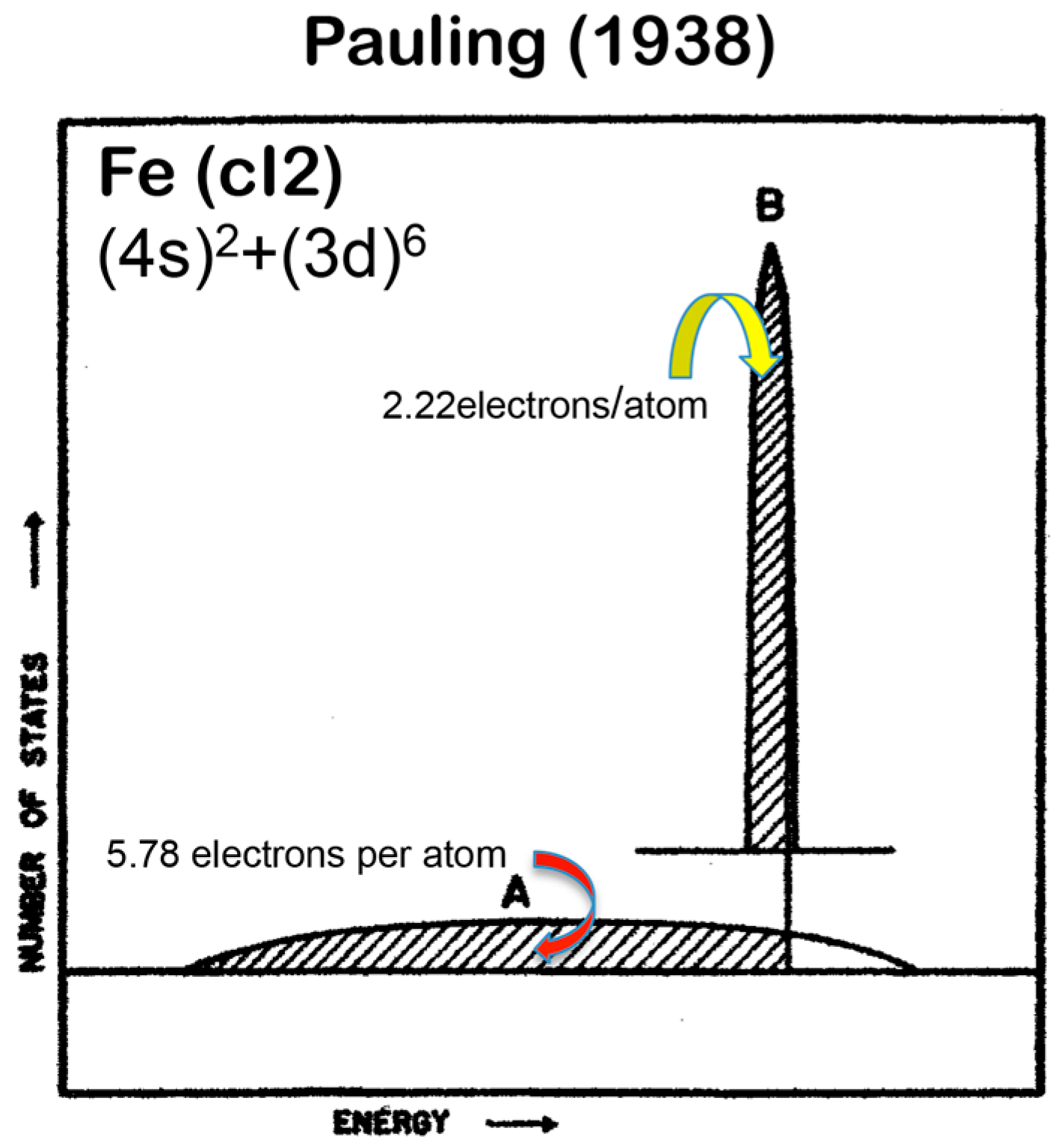
Figure 3.
(a) Formation of bonding and anti-bonding levels due to orbital hybridization between neighboring Al-3p and Mn-3d atomic wave-functions; (b) Formation of a pseudogap between bonding and anti-bonding sub-bands due to orbital hybridizations between Al and Mn atoms in an Al-Mn approximant [11,18].

Figure 4.
Formation of stationary electron waves as a result of interference with periodically arranged ionic potentials [11,14,19].
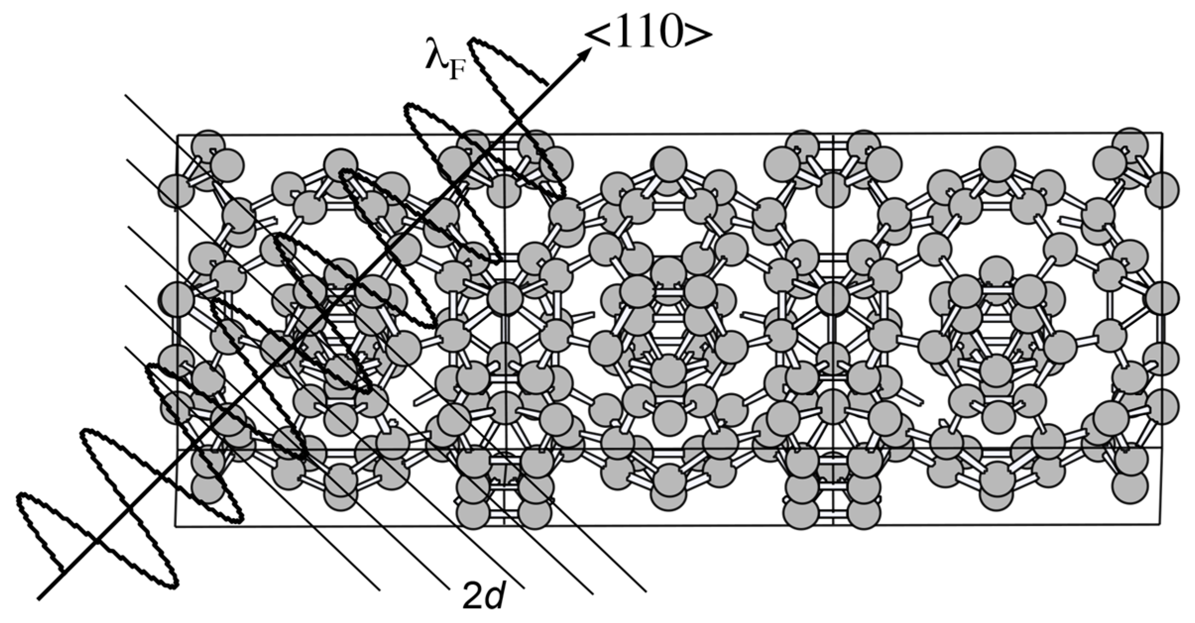
Figure 5.
The FsBz interaction in the Mott and Jones theory [3,11,14,19]. A critical value of (e/a)c is obtained when the Fermi sphere touches the zone plane of the respective Brillouin zones: (a) symmetry points N in the bcc Brillouin zone and (b) the symmetry points N330 and N411 in the bcc Brillouin zone for the gamma-brass structure. Note that the distance from the origin to the points N330 and N411 in (b) is the same and equal to in units of , where a is the lattice constant.
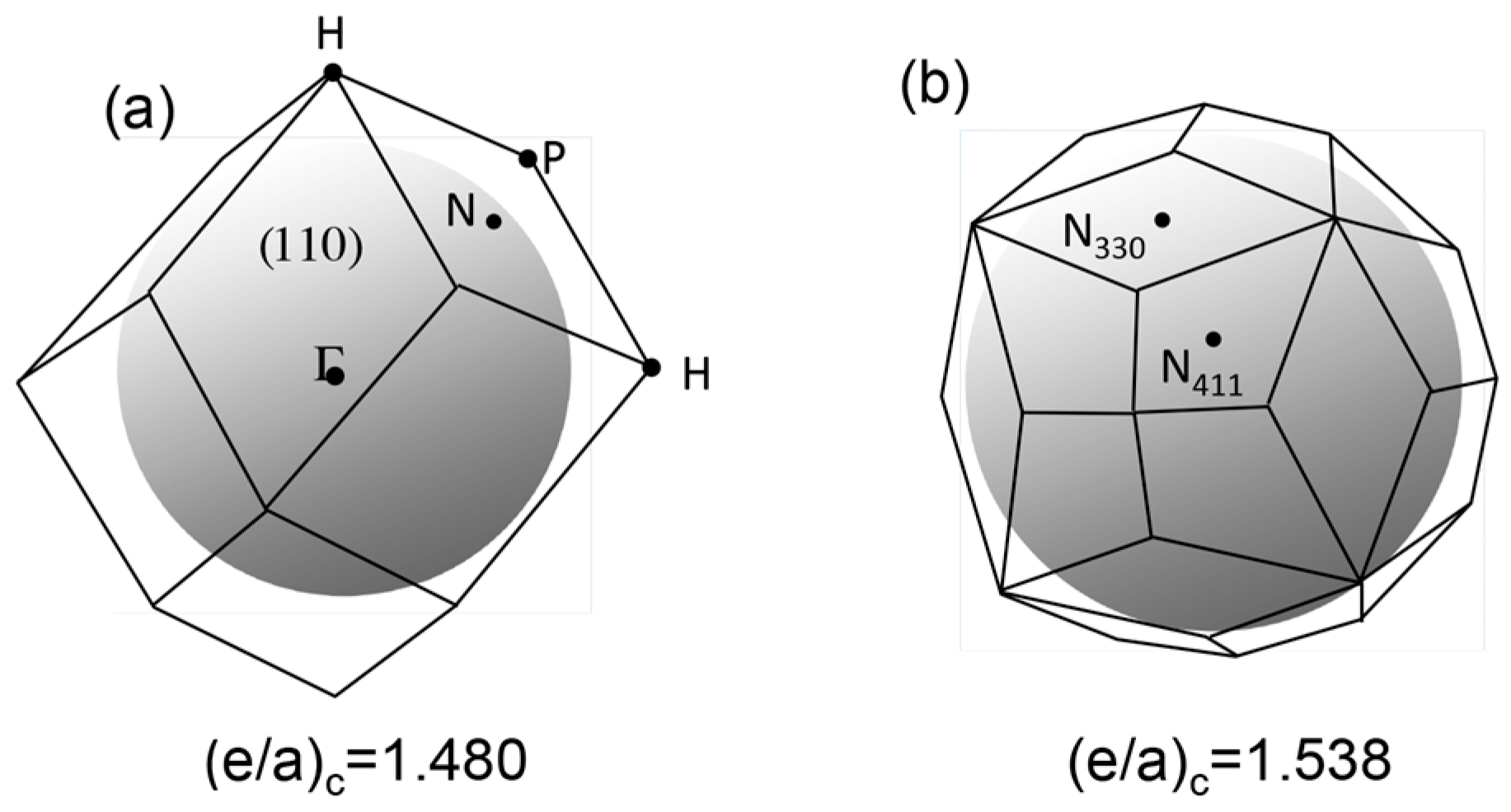
Figure 6.
Seven lattices systems and fourteen Bravais lattices. The Pearson symbol is added in brackets. The right-hand panel shows that hexagonal in the crystal family can be also classified into trigonal and hexagonal with respect to the crystal system.
Figure 6.
Seven lattices systems and fourteen Bravais lattices. The Pearson symbol is added in brackets. The right-hand panel shows that hexagonal in the crystal family can be also classified into trigonal and hexagonal with respect to the crystal system.
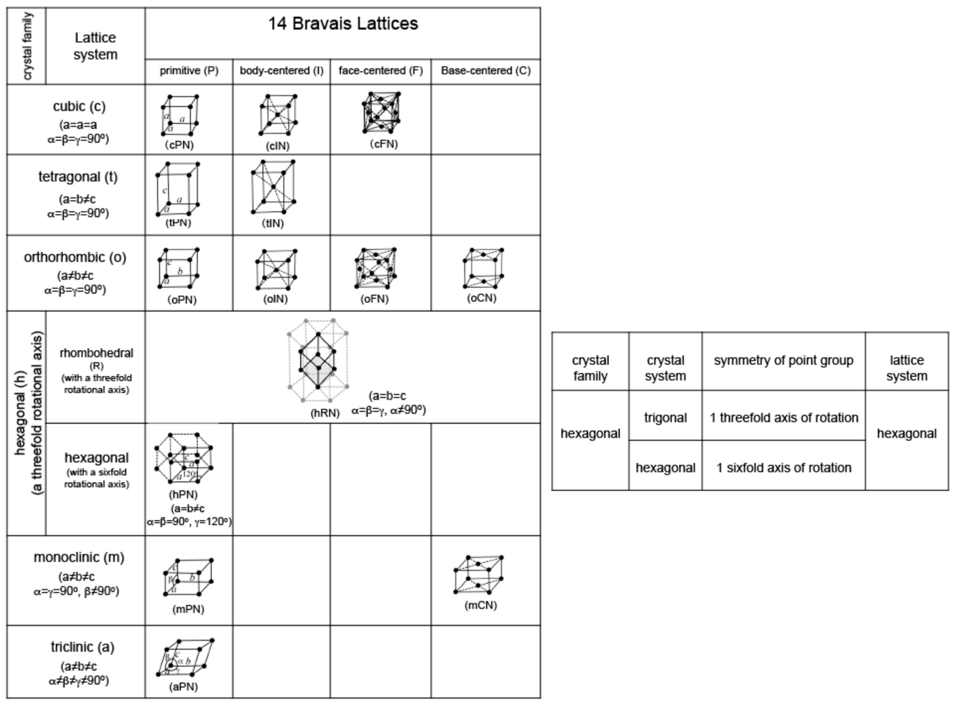
Figure 7.
The first Brillouin zone of (a) simple cubic (sc) lattice; (b) body-centered cubic (bcc) lattice; (c) face-centered cubic (fcc) lattice; (d) hexagonal close packed (hcp) lattice; (e) rhombohedral lattice and (f) base-centered orthorhombic lattice [11].
Figure 7.
The first Brillouin zone of (a) simple cubic (sc) lattice; (b) body-centered cubic (bcc) lattice; (c) face-centered cubic (fcc) lattice; (d) hexagonal close packed (hcp) lattice; (e) rhombohedral lattice and (f) base-centered orthorhombic lattice [11].

Figure 8.
Matrix of the Fourier coefficient, , at the wave vector as functions of the energy eigen-value in column and the reciprocal lattice vector in the electronic state in row.
Figure 8.
Matrix of the Fourier coefficient, , at the wave vector as functions of the energy eigen-value in column and the reciprocal lattice vector in the electronic state in row.

Figure 9.
(a) Dispersion relations; (b) total- and partial-DOSs and (c) Full potential Linearized Augmented Plane Wave (FLAPW)-Fourier spectra at symmetry points Γ, N and H of the bcc Brillouin zone for Na (cI2) [11]. An energy gap across {110} zone planes is marked with red color in (a). Its total-DOS is incorporated in (c).

Figure 10.
(a) Dispersion relations; (b) total- and partial-DOSs and (c) FLAPW-Fourier spectra at symmetry points Γ, L and X of the fcc Brillouin zone for Al (cF4) [11]. Its total-DOS is incorporated in (c).
Figure 10.
(a) Dispersion relations; (b) total- and partial-DOSs and (c) FLAPW-Fourier spectra at symmetry points Γ, L and X of the fcc Brillouin zone for Al (cF4) [11]. Its total-DOS is incorporated in (c).
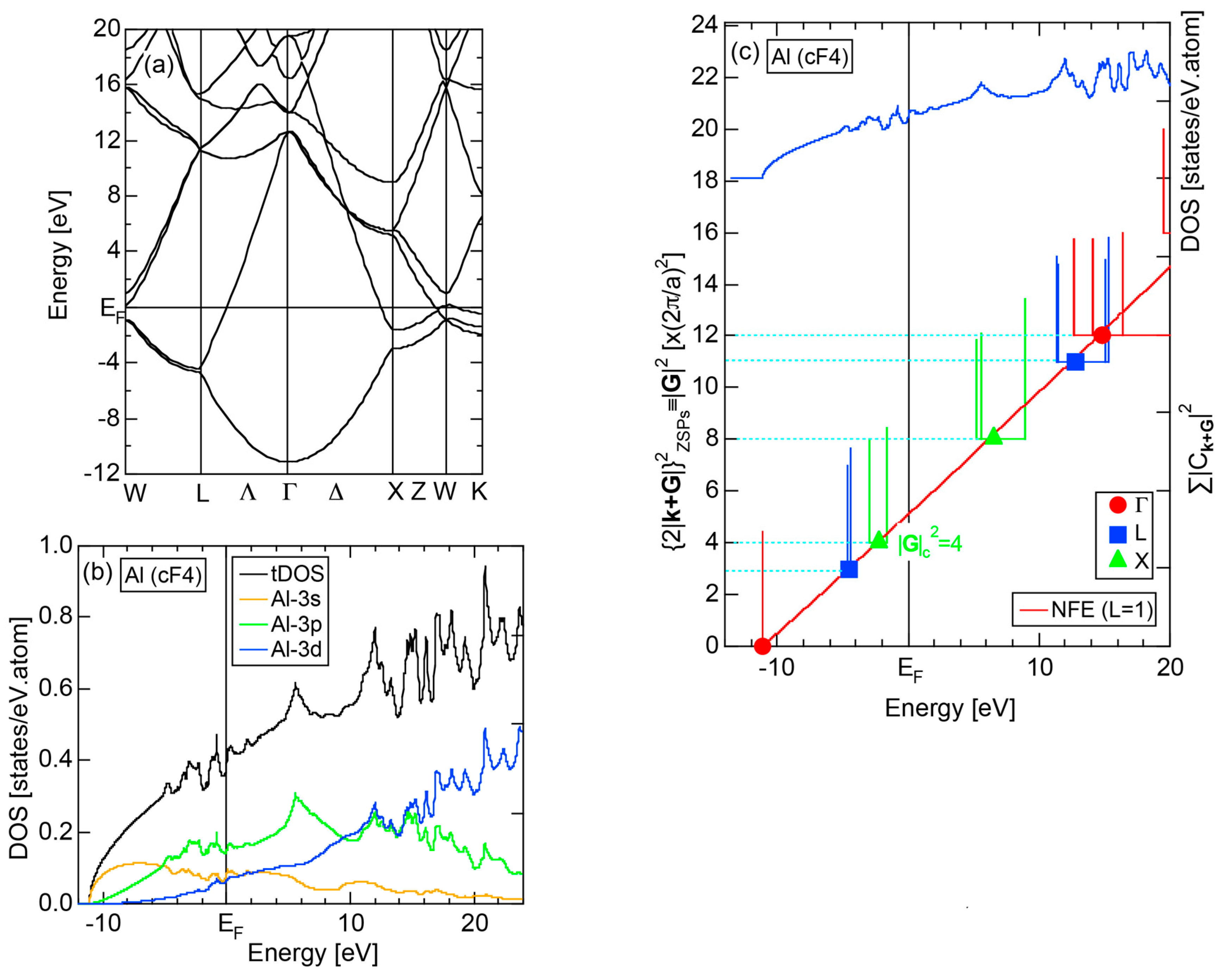
Figure 11.
(a) Dispersion relations; (b) total- and partial-DOSs and (c) FLAPW-Fourier spectra at symmetry points Γ, L and X of the fcc Brillouin zone for Si (cF8) [11]. The total-DOS is incorporated in (c).
Figure 11.
(a) Dispersion relations; (b) total- and partial-DOSs and (c) FLAPW-Fourier spectra at symmetry points Γ, L and X of the fcc Brillouin zone for Si (cF8) [11]. The total-DOS is incorporated in (c).

Figure 12.
(a) Dispersion relations; (b) partial DOSs and (c) FLAPW-Fourier spectra at symmetry points Γ, Z and R of the Brillouin zone for the base-centered orthorhombic lattice for P (oC8) [11]. The total-DOS is incorporated in (c).
Figure 12.
(a) Dispersion relations; (b) partial DOSs and (c) FLAPW-Fourier spectra at symmetry points Γ, Z and R of the Brillouin zone for the base-centered orthorhombic lattice for P (oC8) [11]. The total-DOS is incorporated in (c).

Figure 13.
Partial DOSs for (a) insulating S (mP28) at ambient conditions and (b) metallic S (hR1) synthesized under high pressures P = 206.5 GPa [11]. FLAPW-Fourier spectra at symmetry points Γ, X and M of the Brillouin zone for the monoclinic lattice for (c) insulating S (mP28) and those at symmetry points Γ, L, F and Z of the Brillouin zone for the rhombohedral lattice for metallic S (hR1).
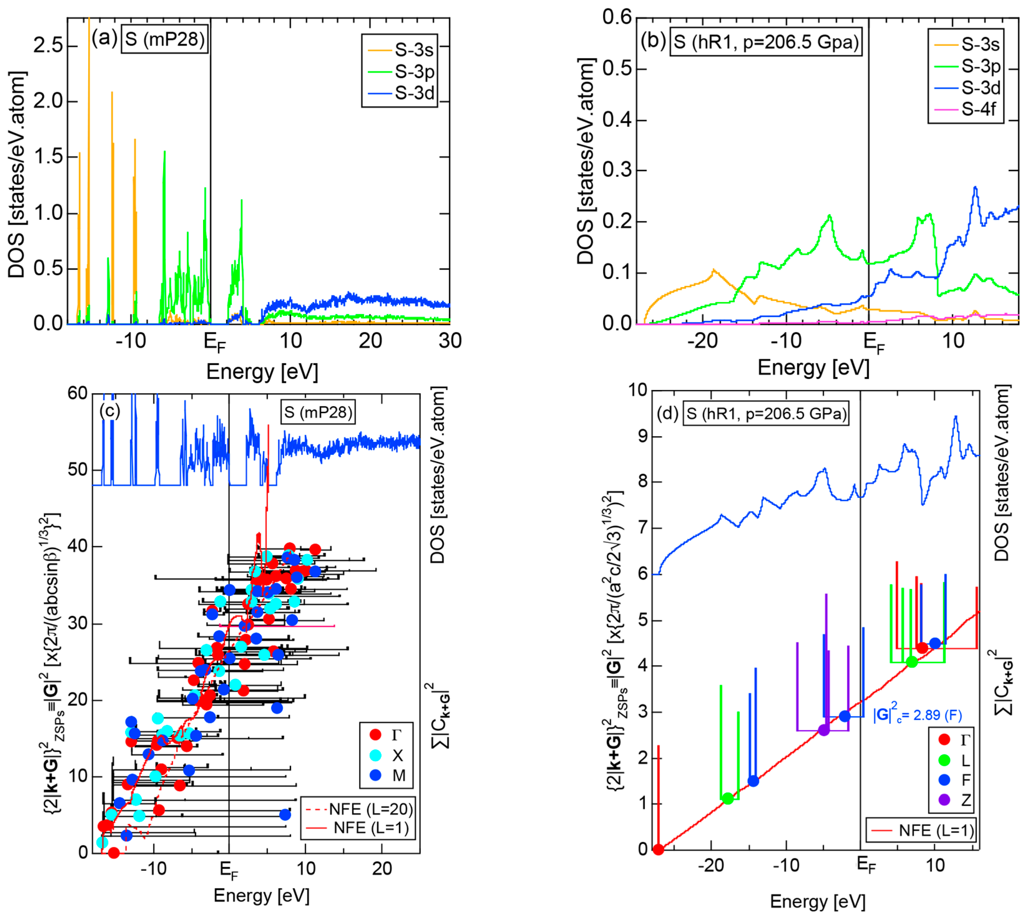
Figure 14.
(a) Dispersion relations; (b) partial DOSs and (c) FLAPW-Fourier spectra at symmetry points Γ, Z and R of the Brillouin zone for the base-centered orthorhombic lattice for insulating solid Cl (oC8) [11]. The total-DOS is incorporated in (c).
Figure 14.
(a) Dispersion relations; (b) partial DOSs and (c) FLAPW-Fourier spectra at symmetry points Γ, Z and R of the Brillouin zone for the base-centered orthorhombic lattice for insulating solid Cl (oC8) [11]. The total-DOS is incorporated in (c).
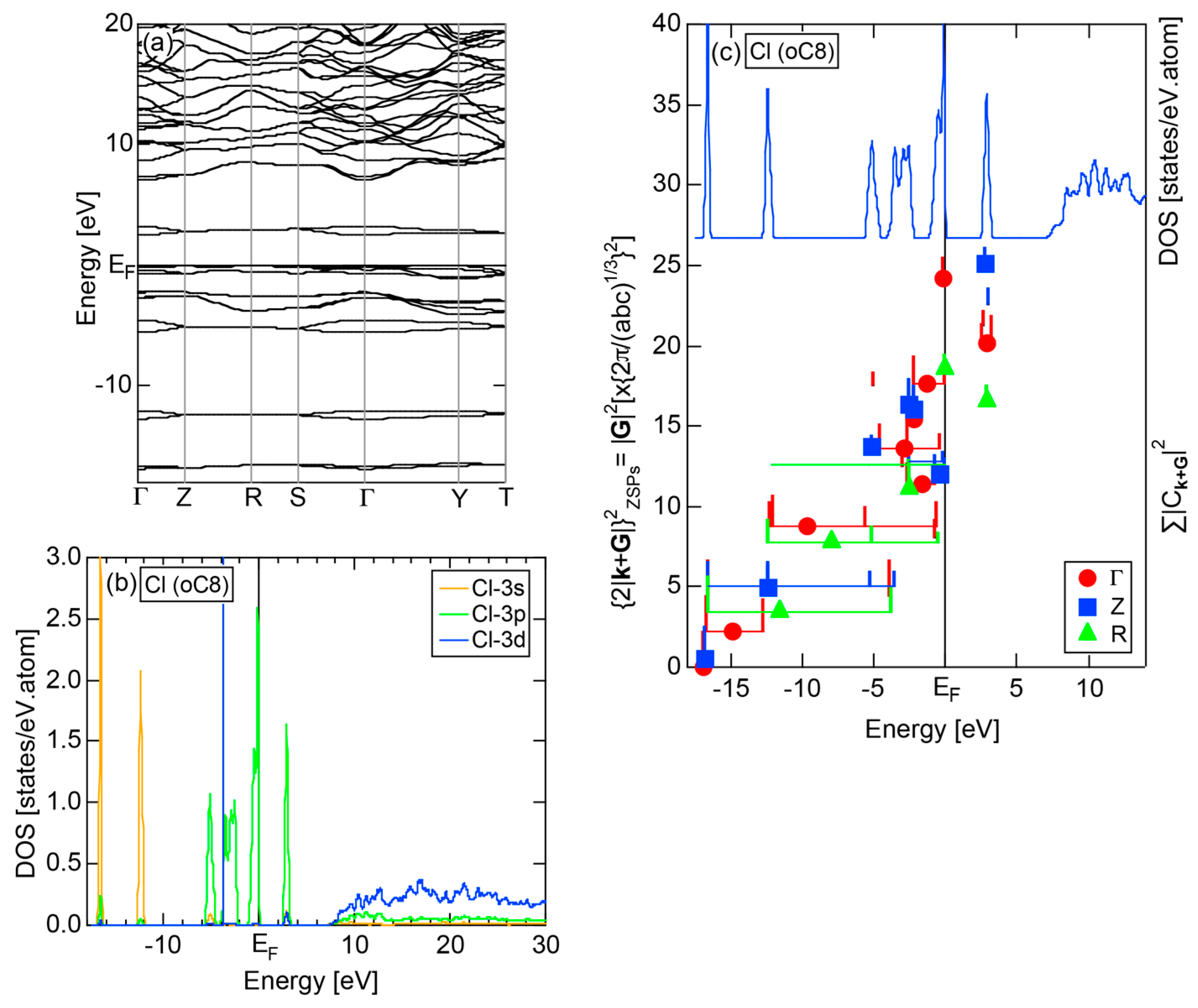
Figure 15.
(a) Partial DOSs; (b) FLAPW-Fourier spectra at symmetry points Γ, R and T of the Brillouin zone for the body-centered orthorhombic lattice for metallic Br (oI2) [11]. The total-DOS is incorporated in (a).
Figure 15.
(a) Partial DOSs; (b) FLAPW-Fourier spectra at symmetry points Γ, R and T of the Brillouin zone for the body-centered orthorhombic lattice for metallic Br (oI2) [11]. The total-DOS is incorporated in (a).
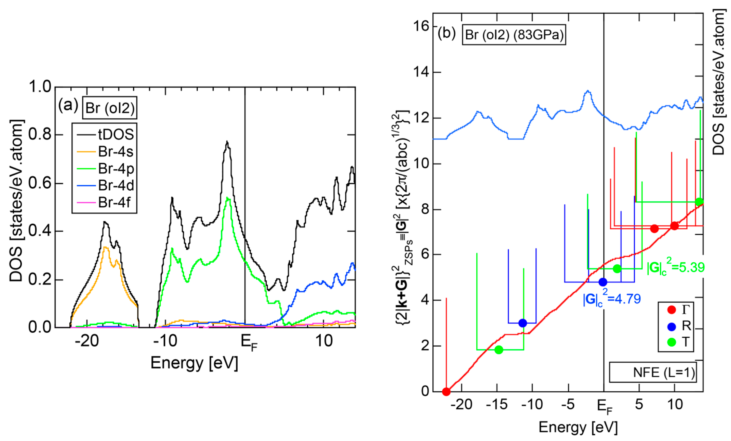
Figure 16.
(a) Dispersion relations; (b) Mn-partial DOSs and (c) FLAPW-Fourier spectra at symmetry points Γ, N and H of the bcc Brillouin zone for α-Mn (cI58) [11]. The total-DOS (blue) and Mn-4p partial DOS (green) are incorporated in (c). Formation of bonding and anti-bonding states due to the Mn-3d-states-mediated splitting is highlighted by yellow color in (c).

Figure 17.
Cross-section of the Fermi surface-Brillouin zone interactions in the extended zone scheme for simple cubic lattice. Some parts of the Fermi sphere enter into the second zone in yellow color but the rest remains in the first zone in grey color. The circular shell sandwiched by double circles represents the cross section of two constant energy surfaces with E and E + ΔE. The electronic state of wave vector in the first zone is transferred to its equivalent state in the second zone with the assistance of the reciprocal lattice vector . Note that multiple energies including are assigned in the state in the framework of the reduced zone scheme, but the energy is solely assigned to the state in the second zone in the framework of the extended zone scheme.
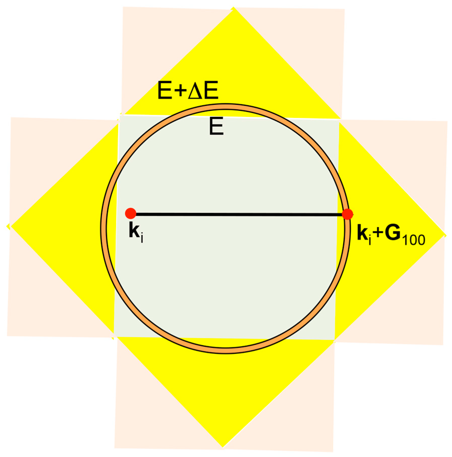
Figure 18.
(a) The Hume-Rothery plot for tri-valent Al (cF4). The data points in red color are contributed from electronic states in the first zone, those in blue from the second zone and those in green from the third zone in the extended zone scheme. Contributions from all three zones coexist over the energy range from −4.4 to −0.5 eV. They are summed up to constitute the Hume-Rothery plot, as shown in Figure 20b in its complete form; (b) The resulting Fermi surface of Al (cF4) in the extended zone scheme. The blue and green colors are chosen to represent the Fermi surfaces overlapped into the second and third zones so as to meet with colors in (a), respectively.

Figure 19.
(a) and (b) Hume-Rothery plot for Na (cI2) [11]. Symbols in (b) refer to the TH-HR (Tetrahedron-Hume-Rothery) data points (black), dimensionless variance F(E) (grey), nearly free electron (NFE) curve (L = 1) (red), and data points satisfying the condition (green dots).
Figure 19.
(a) and (b) Hume-Rothery plot for Na (cI2) [11]. Symbols in (b) refer to the TH-HR (Tetrahedron-Hume-Rothery) data points (black), dimensionless variance F(E) (grey), nearly free electron (NFE) curve (L = 1) (red), and data points satisfying the condition (green dots).

Figure 20.
(a) and (b) Hume-Rothery plot for Al (cF4) [11]. See captions of Figure 19b for symbols in (b).

Figure 21.
(a) and (b) Hume-Rothery plot for Si (cF8) [11]. See captions of Figure 19b for symbols in (b).
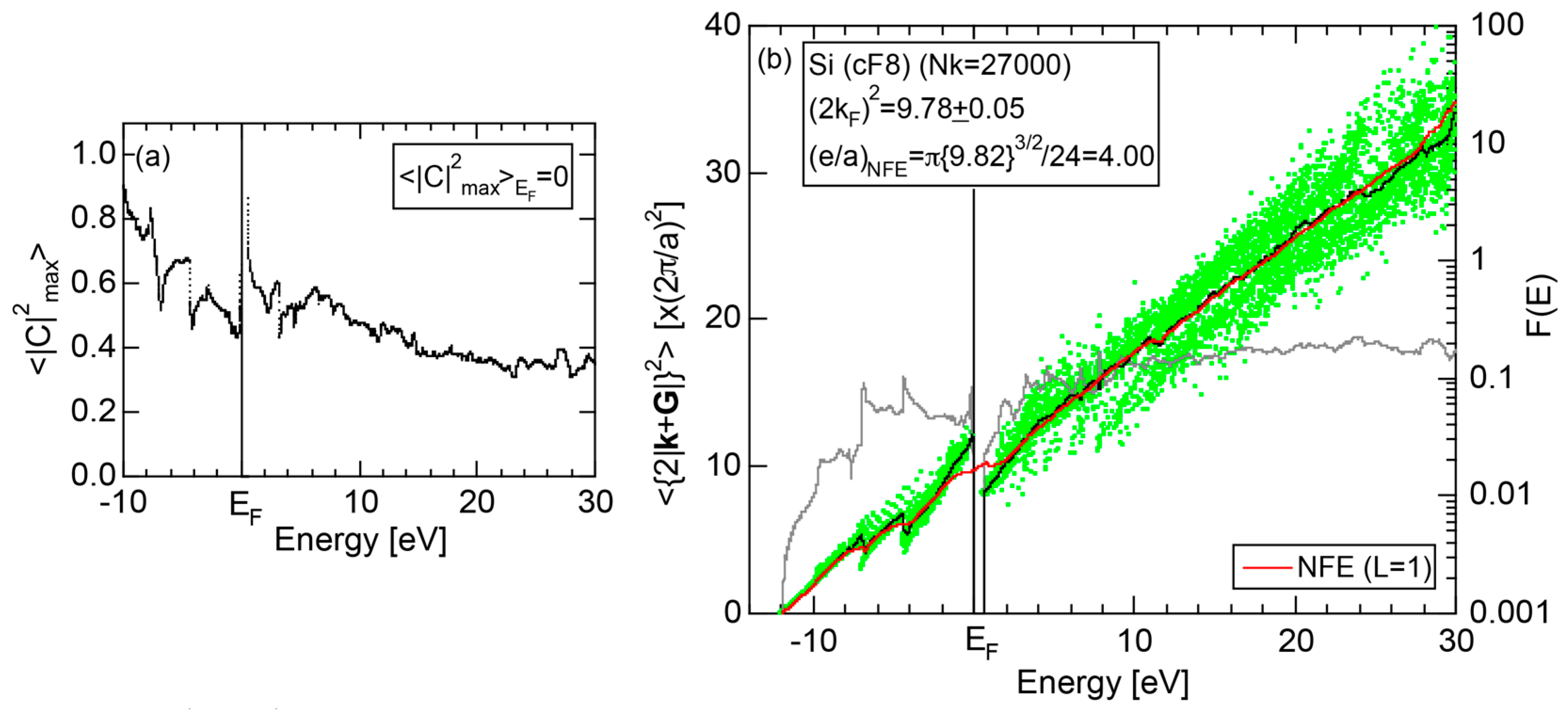
Figure 22.
(a) and (b) Hume-Rothery plot for P (oC8) [11]. See captions of Figure 19b for symbols in (b).

Figure 23.
(a,c) and (b,d) Hume-Rothery plot for insulating S (mP28) and metallic S (hR1), respectively [11]. See captions of Figure 19b for symbols in (b) and (d).
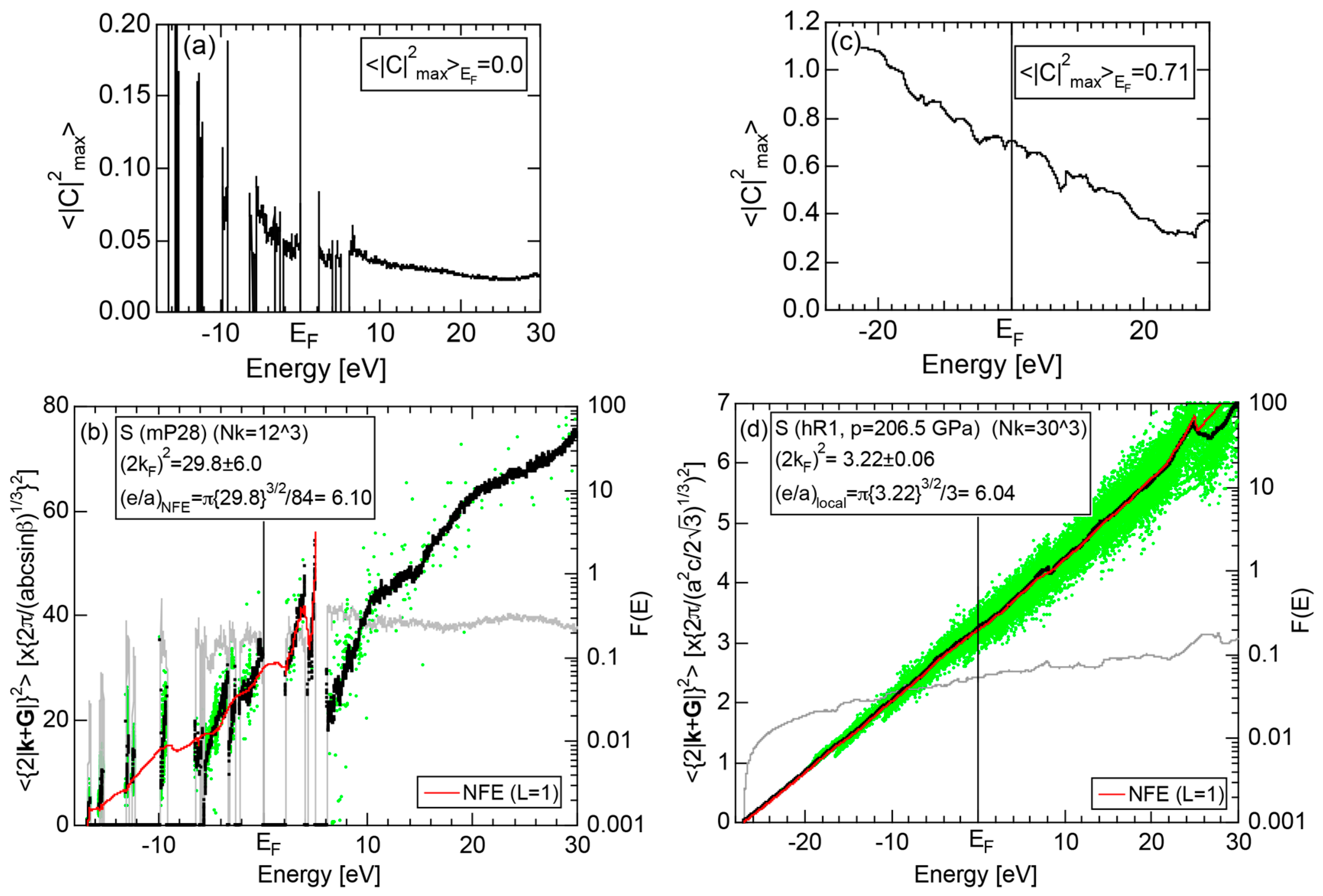
Figure 24.
(a) and (b) Hume-Rothery plot for insulating solid Cl (oC8) [11]. See captions of Figure 19b for symbols in (b).
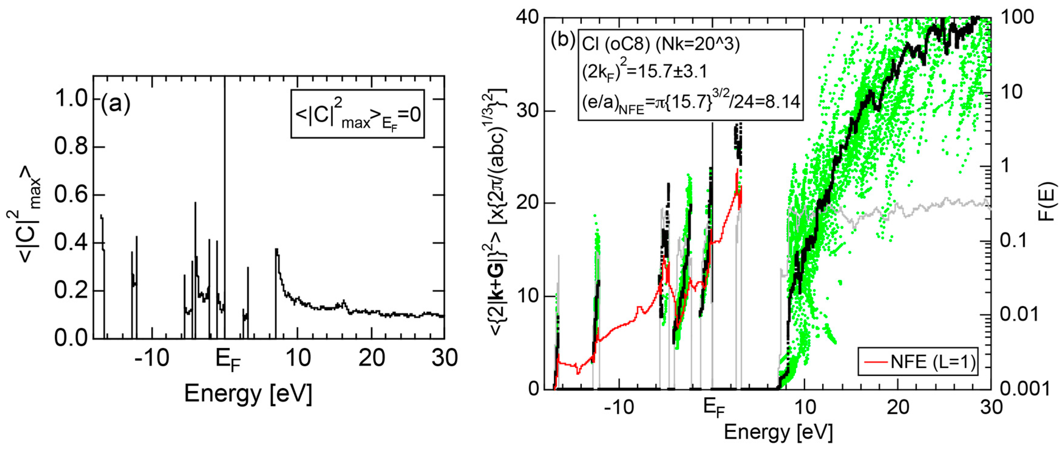
Figure 25.
(a) and (b) Hume-Rothery plot for metallic Br (oI2) synthesized under P = 83 GPa [11]. See captions of Figure 19b for symbols in (b).
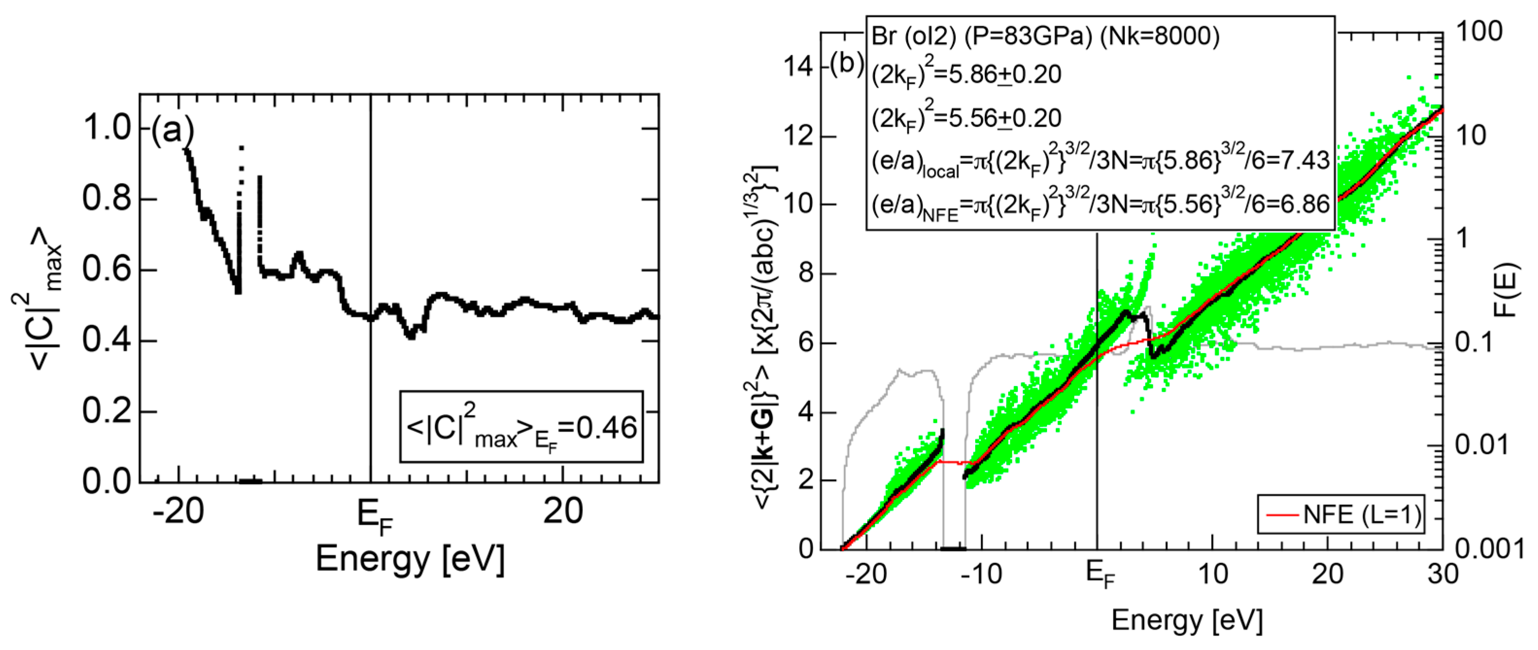
Figure 26.
(a) and (b) Hume-Rothery plot for α-Mn (cI58) [11]. See captions of Figure 19b for symbols in (b).

Figure 27.
Allen’s multiplet-averaged energy () of free atoms in comparison with of expanded elements with a = 2a0 () and that of elements with a = a0 (). a0: lattice constant of elements under normal conditions. See Equation (16) for the definition of and for an element A.
Figure 27.
Allen’s multiplet-averaged energy () of free atoms in comparison with of expanded elements with a = 2a0 () and that of elements with a = a0 (). a0: lattice constant of elements under normal conditions. See Equation (16) for the definition of and for an element A.
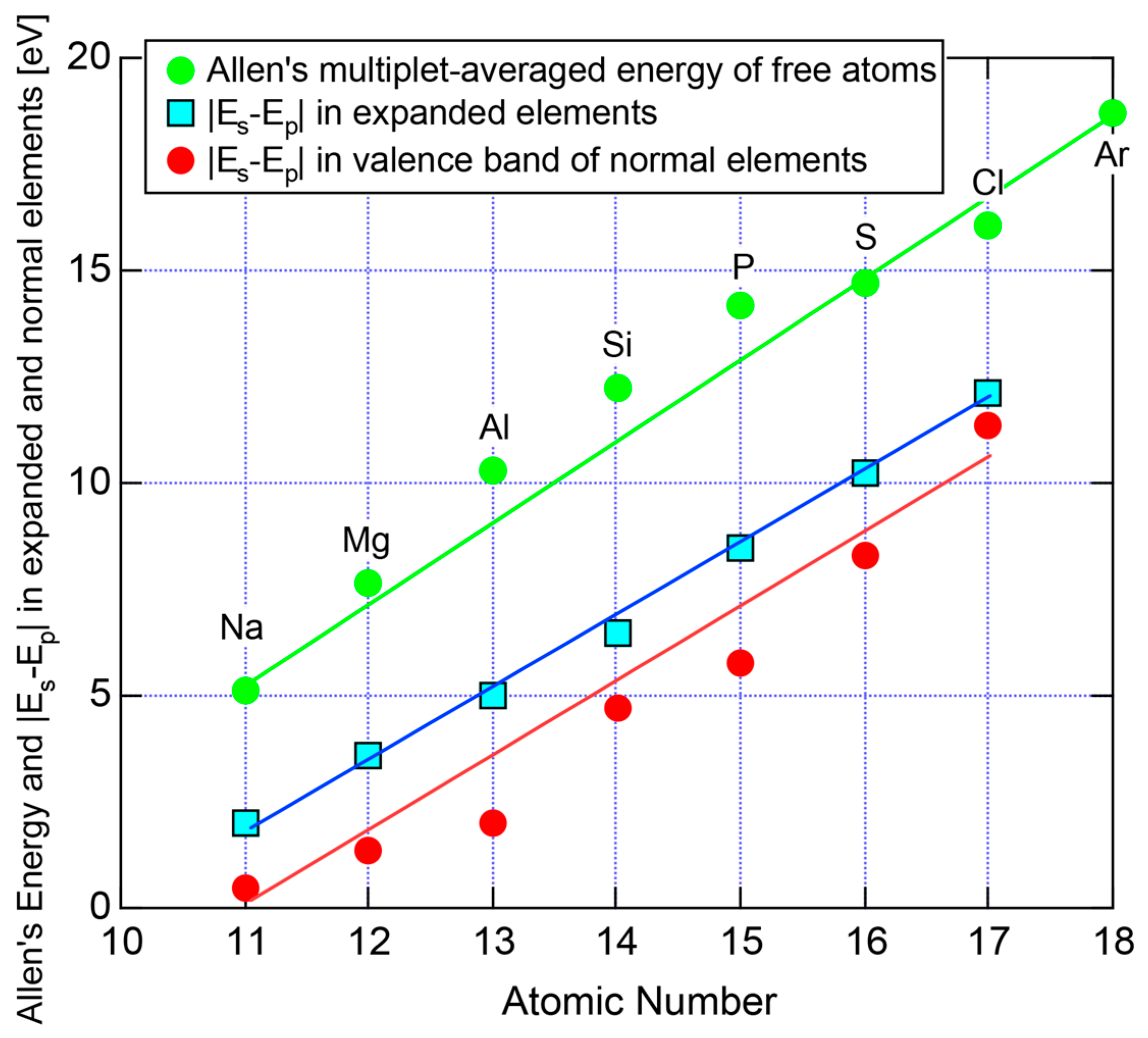
Figure 28.
(a) Na-partial DOSs and its separation energy for bcc Na (cI2) and (b) Cl-partial DOSs and its separation energy for orthorhombic Cl (oS8) [11,12].

Figure 29.
Van Arkel-Ketelaar triangle map constructed by inserting the Allen electronegativity data (Table 2) into Equations (17) and (18) for 28 equiatomic compounds and seven elements (○) in period 3 of the Periodic Table [11,12]. The equiatomic Zintl compounds AX (A = Li and Na and X =Al, Ga, In, and Tl) () and Al-, Zn- and Cd-TM compounds () and P-based compounds ().

Figure 30.
Atomic number dependence of (a) FLAPW separation energy and (b) Allen electronegativity for elements in periods 3 and 4 of the Periodic Table [11,12].
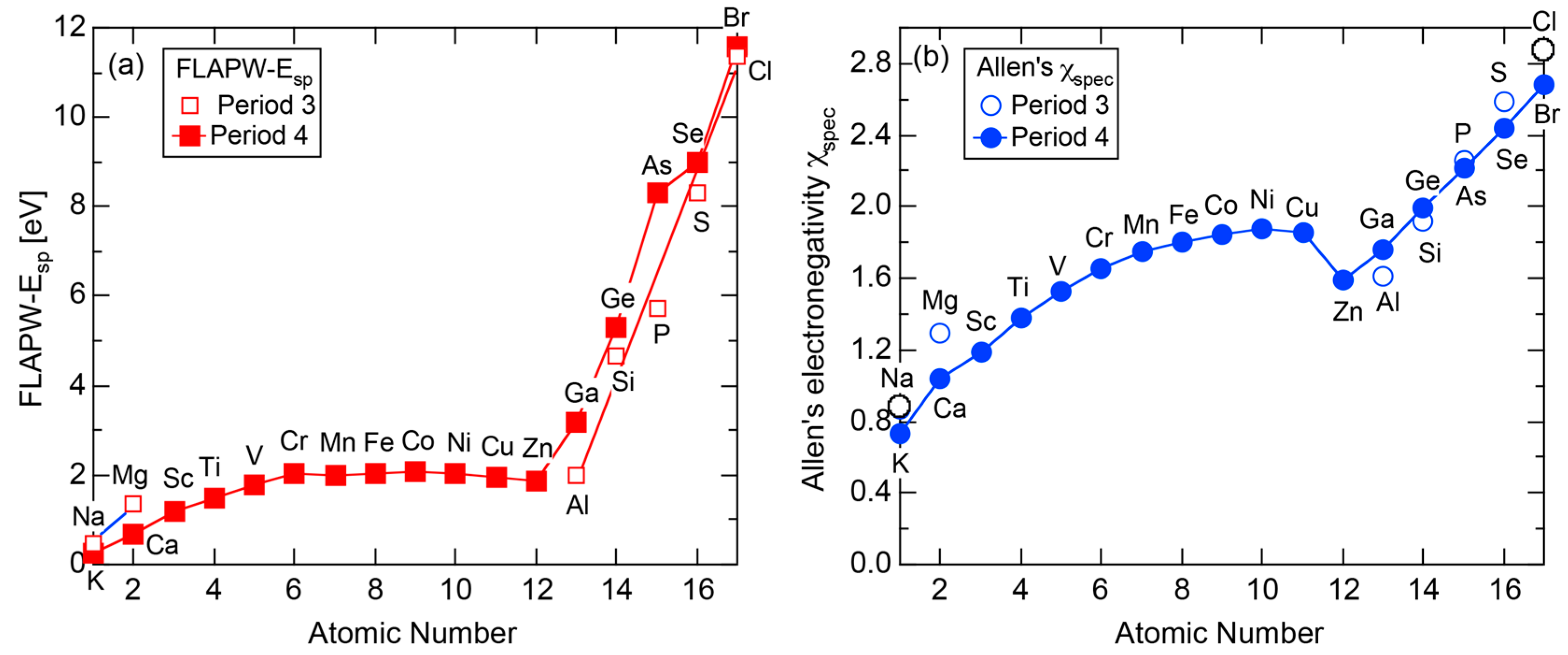
Figure 31.
Van Arkel-Ketelaar triangle map for Al-, Zn- and Cd-based equiatomic compounds. It was constructed by inserting Allen’s electronegativity data (Table 2) into Equations (17) and (18) [12].
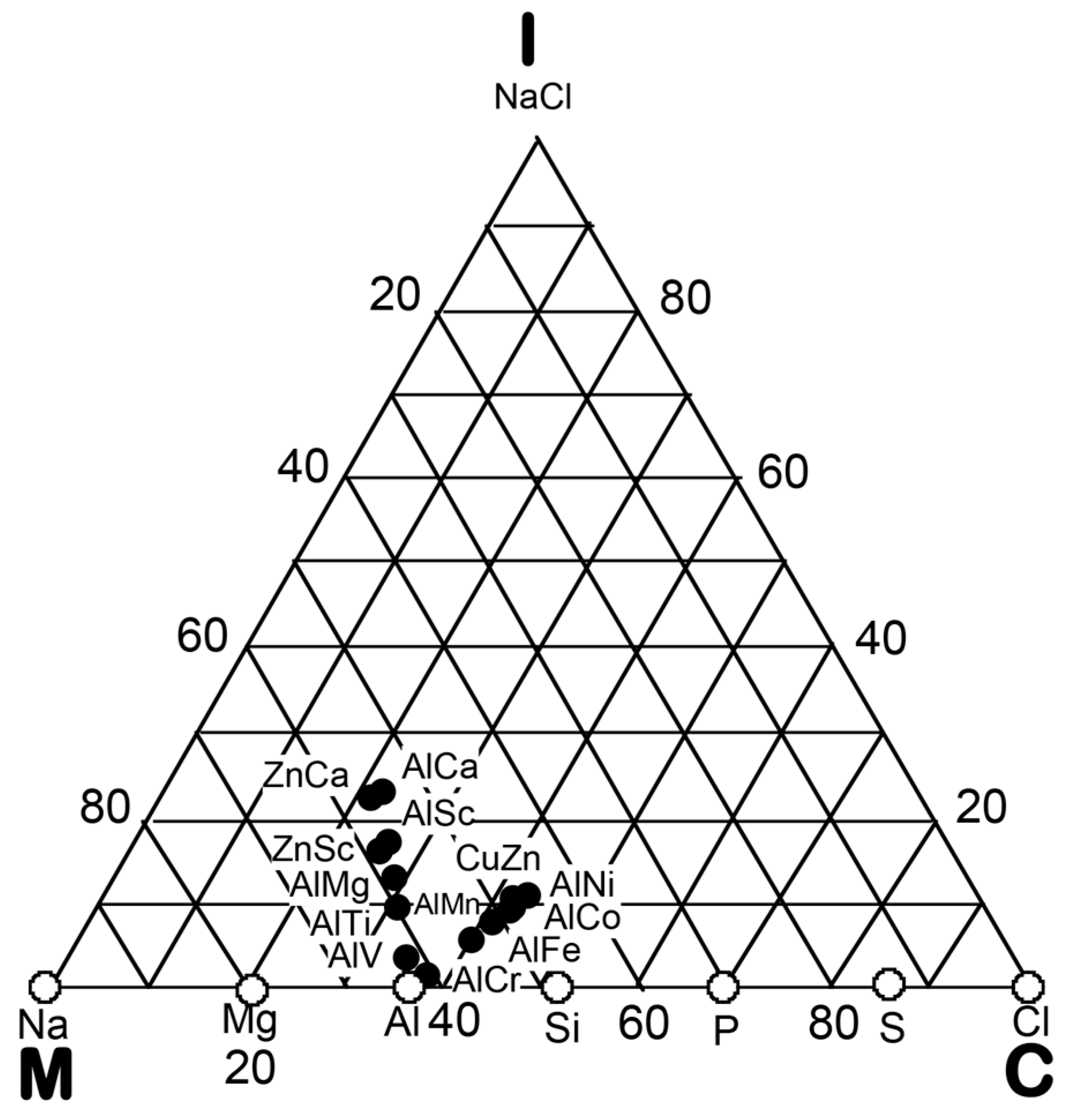
Figure 32.
(a) Cu- and (b) Zn-pDOSs for Cu5Zn8 (cI52) and (c) Al- and (d) Cu-pDOSs for Al4Cu9 (cP52).
Figure 32.
(a) Cu- and (b) Zn-pDOSs for Cu5Zn8 (cI52) and (c) Al- and (d) Cu-pDOSs for Al4Cu9 (cP52).

Figure 33.
(a) Al- and (b) V-pDOSs for Al8V5 (cI52) and (c) Ag- and (d) Li-pDOSs for Ag5Li8 (cI52).
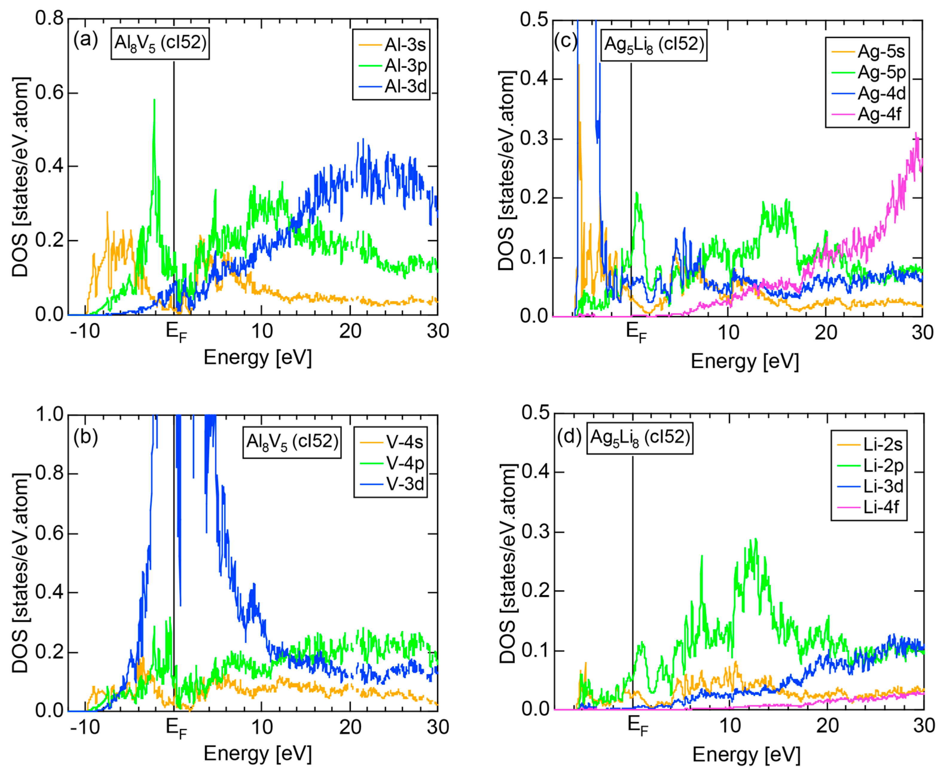
Figure 34.
(a) and (b) Hume-Rothery plot for Cu5Zn8 (cI52) [11]. Respective data in (c,d) for Al4Cu9 (cP52). Symbols in (b,d) refer to the TH-HR (Tetrahedron-Hume-Rothery) data points (black), dimensionless variance F(E) (grey), NFE curve (L = 1) (dotted grey), and data points satisfying the condition (green dots). The NFE curve in (b,d) is intentionally shown with less visible grey dots, since the local reading method is used.
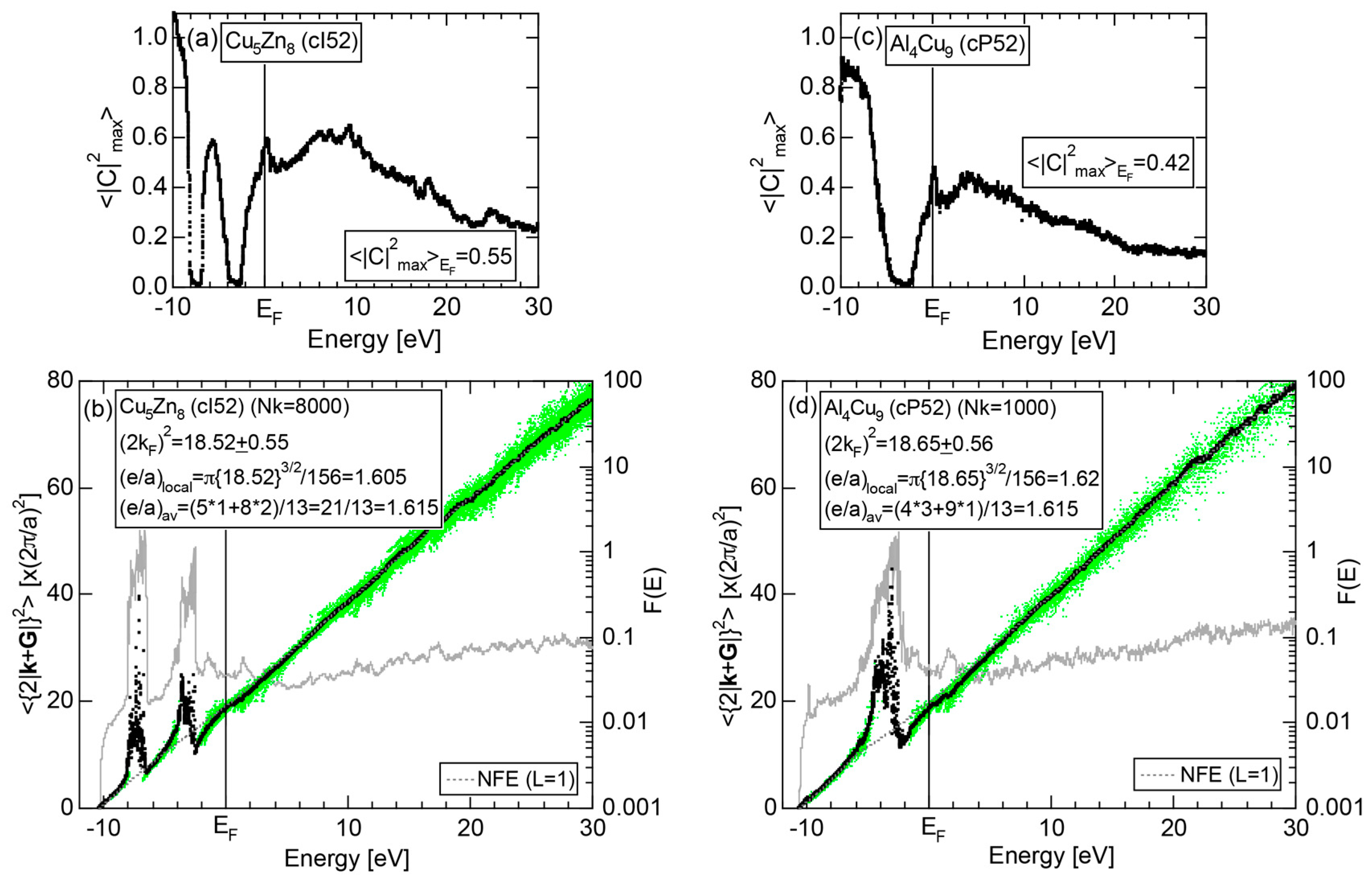
Figure 35.
(a) and (b) Hume-Rothery plot for Al8V5 (cI52). Respective data in (c,d) for Ag5Li8 (cP52). See captions of Figure 34b,d for symbols. The NFE curve in (b) is drawn with red color, since the NFE method is used.
Figure 35.
(a) and (b) Hume-Rothery plot for Al8V5 (cI52). Respective data in (c,d) for Ag5Li8 (cP52). See captions of Figure 34b,d for symbols. The NFE curve in (b) is drawn with red color, since the NFE method is used.
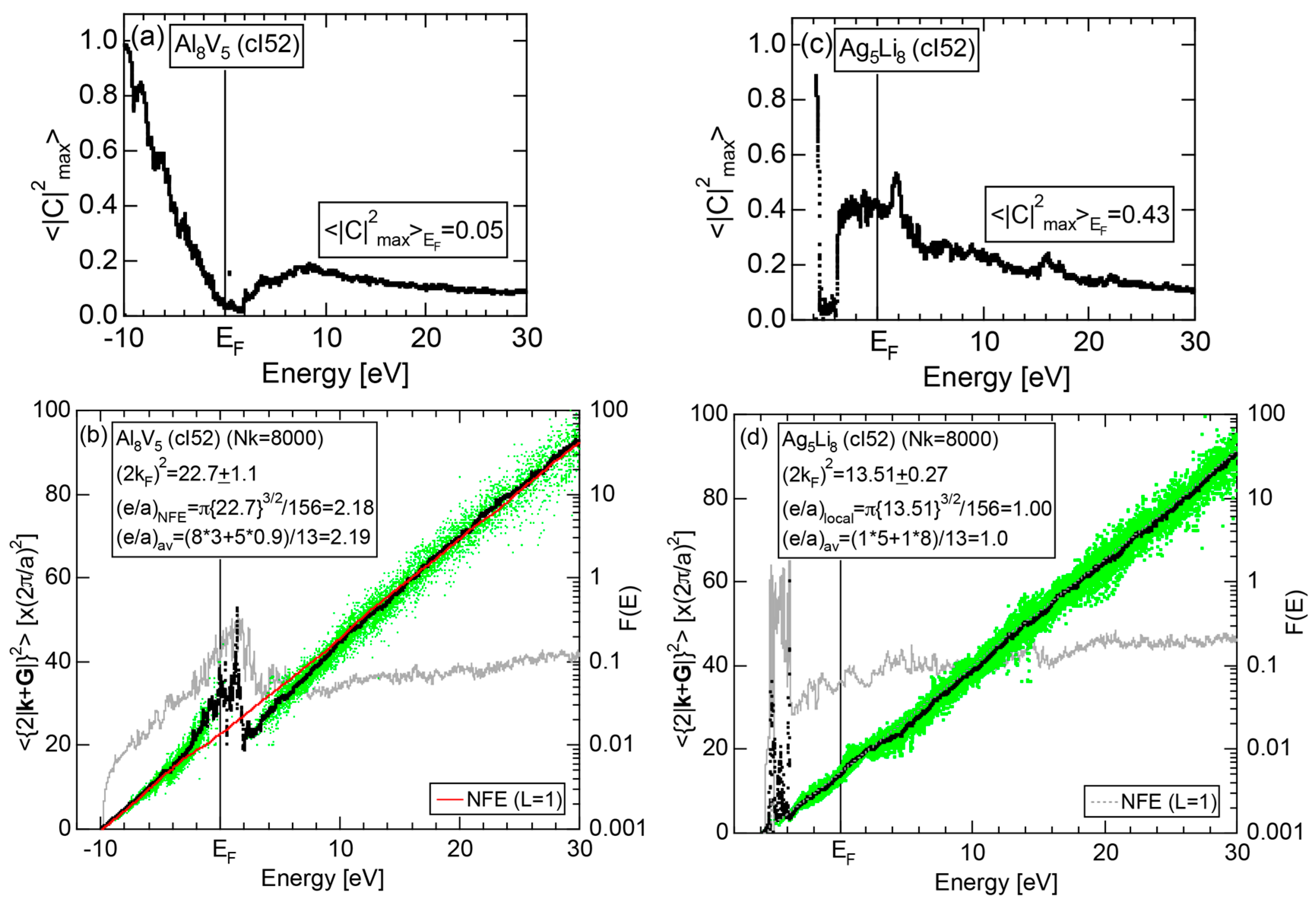
Figure 36.
(a) FLAPW-Fourier spectra at symmetry points N of the bcc Brillouin zone along with the total DOS for Cu5Zn8 (cI52) and (b) those at symmetry points M of the simple cubic (sc) lattice Brillouin zone for Al4Cu9 (cP52) [11].
Figure 36.
(a) FLAPW-Fourier spectra at symmetry points N of the bcc Brillouin zone along with the total DOS for Cu5Zn8 (cI52) and (b) those at symmetry points M of the simple cubic (sc) lattice Brillouin zone for Al4Cu9 (cP52) [11].

Figure 37.
(a) The -dependence of the Fourier-transformed empty-core potential or the form factor, VG, calculated in the context of NFE band calculations for Cu5Zn8 (cI52) gamma-brass [19]; (b) The Fermi surface in the extended zone scheme for Cu5Zn8 (cI52) gamma-brass. Blue dots represent the center of {330} and {411} zone planes. The highest energy is attained at the point “A” on the Brillouin zone. Star-shape pink areas with their centers underneath the point “A” represent spherical Fermi surface inside the Brillouin zone, while white areas the necks formed around centers of the respective zone planes.

Figure 38.
FLAPW-Fourier spectra at symmetry points Γ, N and H of the bcc Brillouin zone along with the total DOS for (a) Al8V5 (cI52) and (b) Ag5Li8 (cI52). A green curve in (a) represents the Al-3p pDOS. Formation of bonding and anti-bonding states due to V-3d-states-mediated splitting is highlighted by yellow color in (a). An orange vertical line in (b) is drawn so as to pass the energy corresponding to the center of gravity energy state with = 18. It meets the pseudogap in the total DOS in Ag5Li8 (cI52).

Figure 39.
(a) Total-DOSs; (b) Hume-Rothery plots and (c) FLAPW-Fourier spectra at symmetry points N of the bcc Brillouin zone for Al3Mg4Zn3 (cI160) (red) and Al9Mg8Ag3 (cI160) (blue) [11,13].

Figure 40.
(a) Total DOSs; (b) Hume-Rothery plots and (c) FLAPW-Fourier spectra at symmetry points N of the bcc Brillouin zone for Al21Li13Cu6 (cI160) (red) and Ga21Li13Cu6 (cI160) (blue) [11,13].
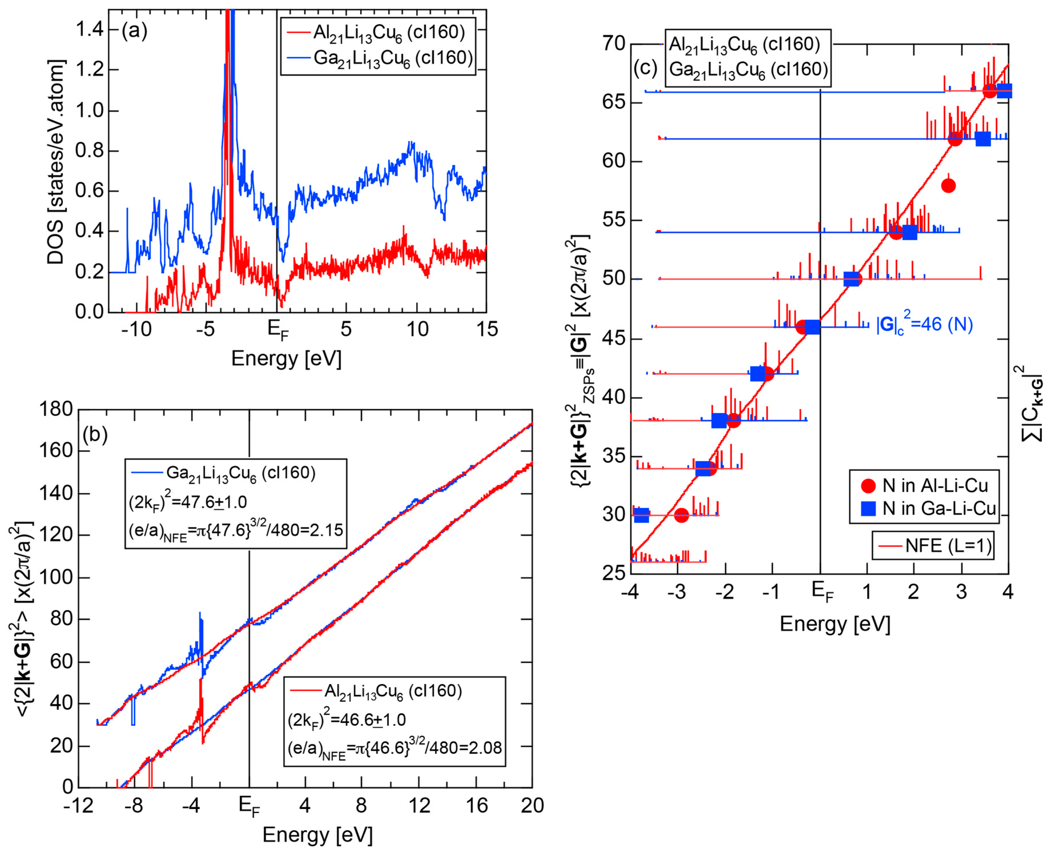
Figure 41.
(a) Total DOSs; (b) Hume-Rothery plots and (c) FLAPW-Fourier spectra at symmetry points Γ, M, X of simple cubic Brillouin zone for Al13Mg27Zn45 (cP680) (red) and Na27Mg27Zn45 (cP680) [11,13].

Figure 42.
(a) The Al-3s, Al-3p and Mn-3d pDOSs; (b) and (c) Hume-Rothery plot for Al114Mn24 (cP138) [11,18]. See captions of Figure 19 b for symbols in (c).

Figure 43.
FLAPW-Fourier spectra at symmetry points Γ, M, X of simple cubic Brillouin zone for Al114Mn24 (cP138) [11,18]. Formation of bonding and anti-bonding states due to Mn-3d-states-mediated splitting is highlighted by yellow color.
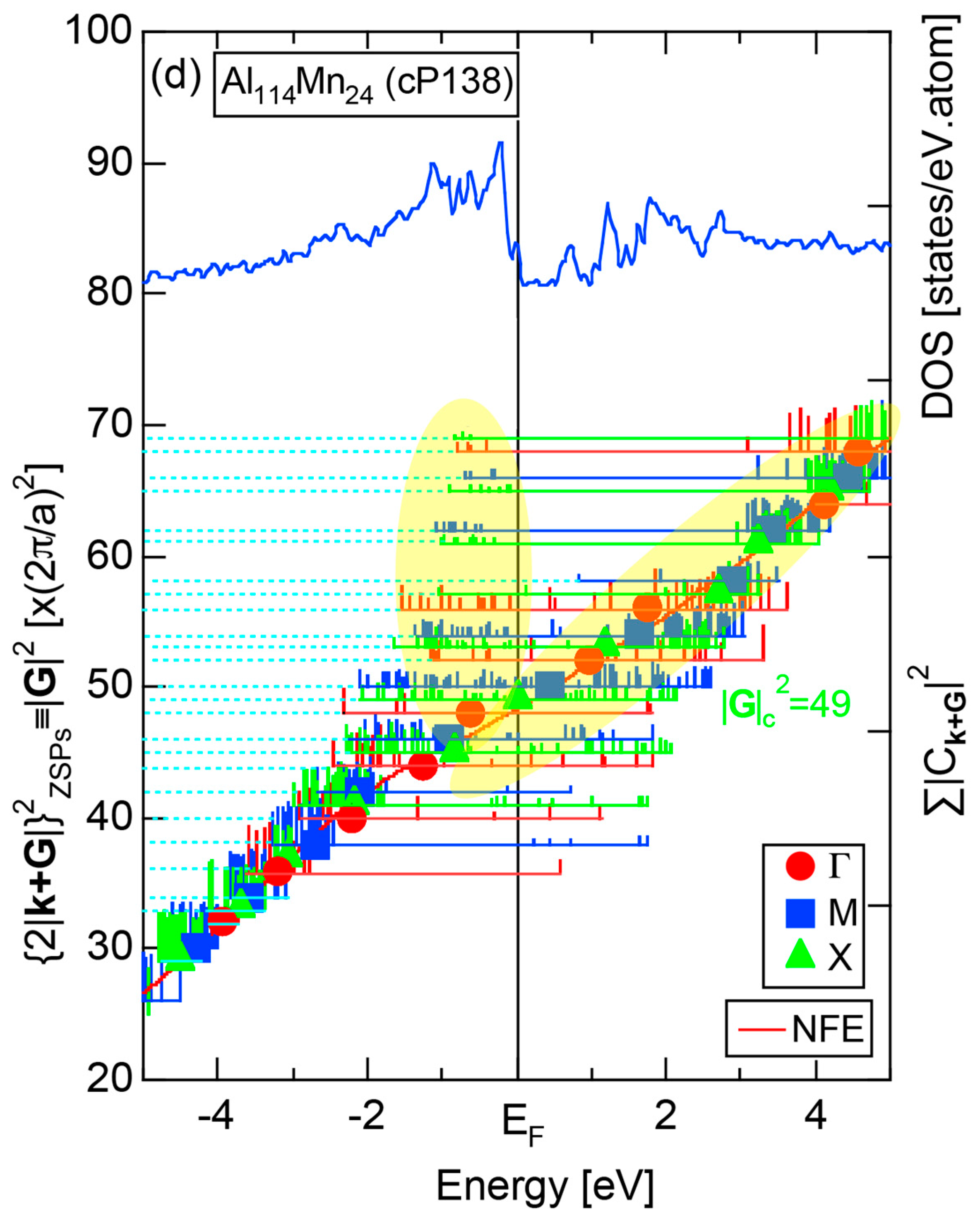
Figure 44.
(a) Total DOSs and Al-3spd pDOSs; (b) Hume-Rothery plot and (c) FLAPW-Fourier spectra at symmetry points Γ, M, X of simple cubic Brillouin zone for Al108Cu9Fe24Si6 (cP144) [11].
Figure 44.
(a) Total DOSs and Al-3spd pDOSs; (b) Hume-Rothery plot and (c) FLAPW-Fourier spectra at symmetry points Γ, M, X of simple cubic Brillouin zone for Al108Cu9Fe24Si6 (cP144) [11].

Figure 45.
(a) Cd- and (b) Ca-pDOSs; (c) Hume-Rothery plot and (d) FLAPW-Fourier spectra at symmetry points Γ, M, X of simple cubic Brillouin zone for Cd6Ca (cP168) [11,45]. A blue curve in (d) indicates the total-DOS.

Figure 46.
(a) Cd- and (b) Yb-pDOSs; (c) Hume-Rothery plot and (d) FLAPW-Fourier spectra at symmetry points Γ, N, H of the bcc Brillouin zone for Cd6Yb (cI168) [11]. A blue curve in (d) indicates the total-DOS.
Figure 46.
(a) Cd- and (b) Yb-pDOSs; (c) Hume-Rothery plot and (d) FLAPW-Fourier spectra at symmetry points Γ, N, H of the bcc Brillouin zone for Cd6Yb (cI168) [11]. A blue curve in (d) indicates the total-DOS.
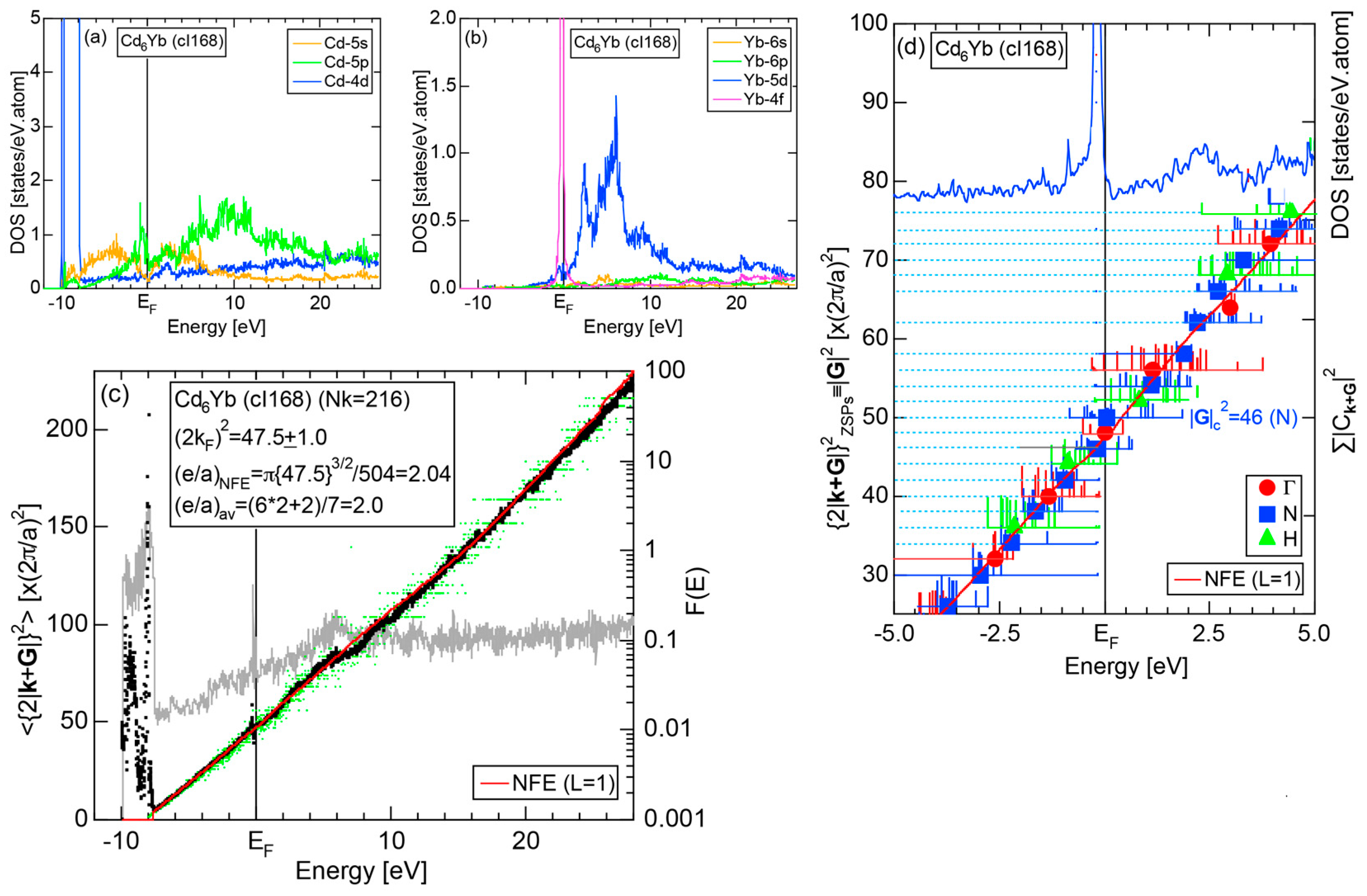
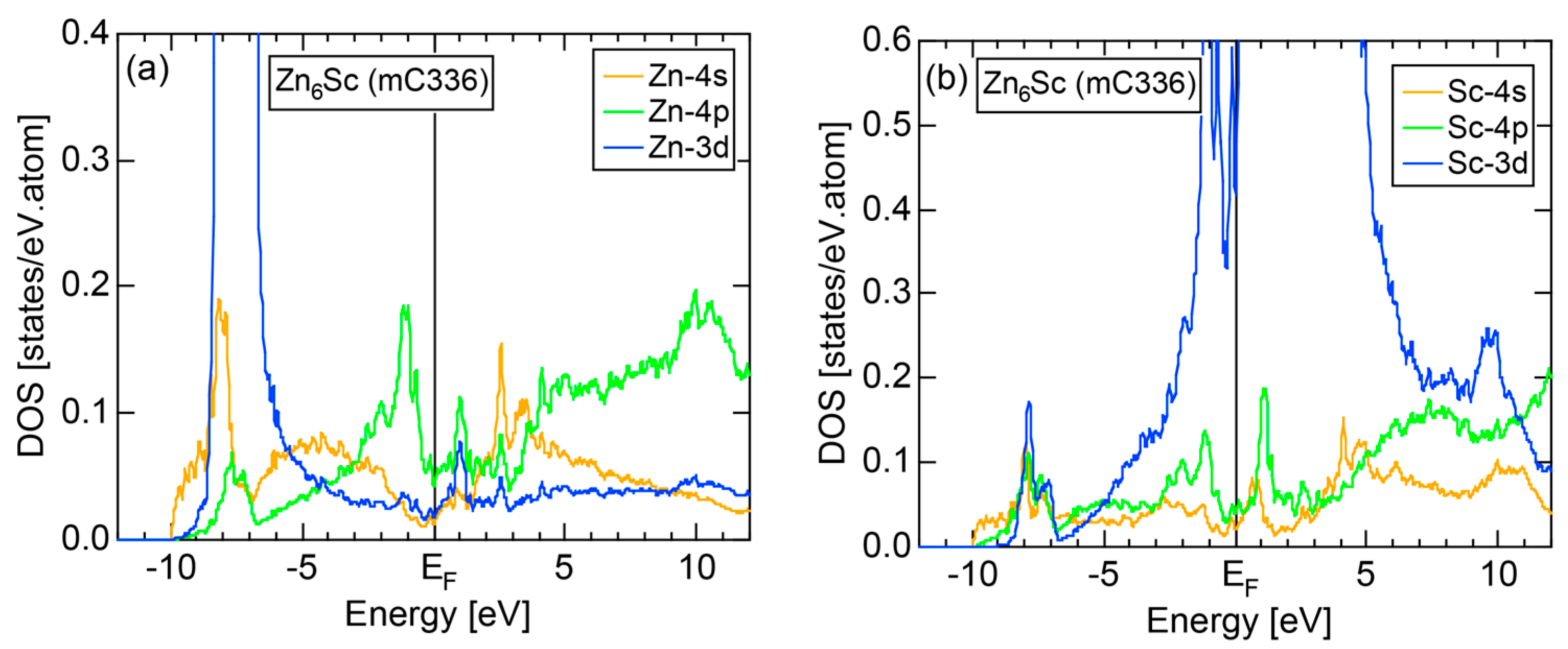
Figure 48.
(a) FLAPW-Fourier spectra at symmetry points Γ, A, Z of the Brillouin zone of monoclinic lattice; (b) and (c) Hume-Rothery plot for Zn6Sc (mC336) [11,50]. Formation of bonding and anti-bonding states due to Sc-3d-states-mediated splitting in (a) is highlighted by yellow color. A blue curve in (a) indicates the total-DOS.

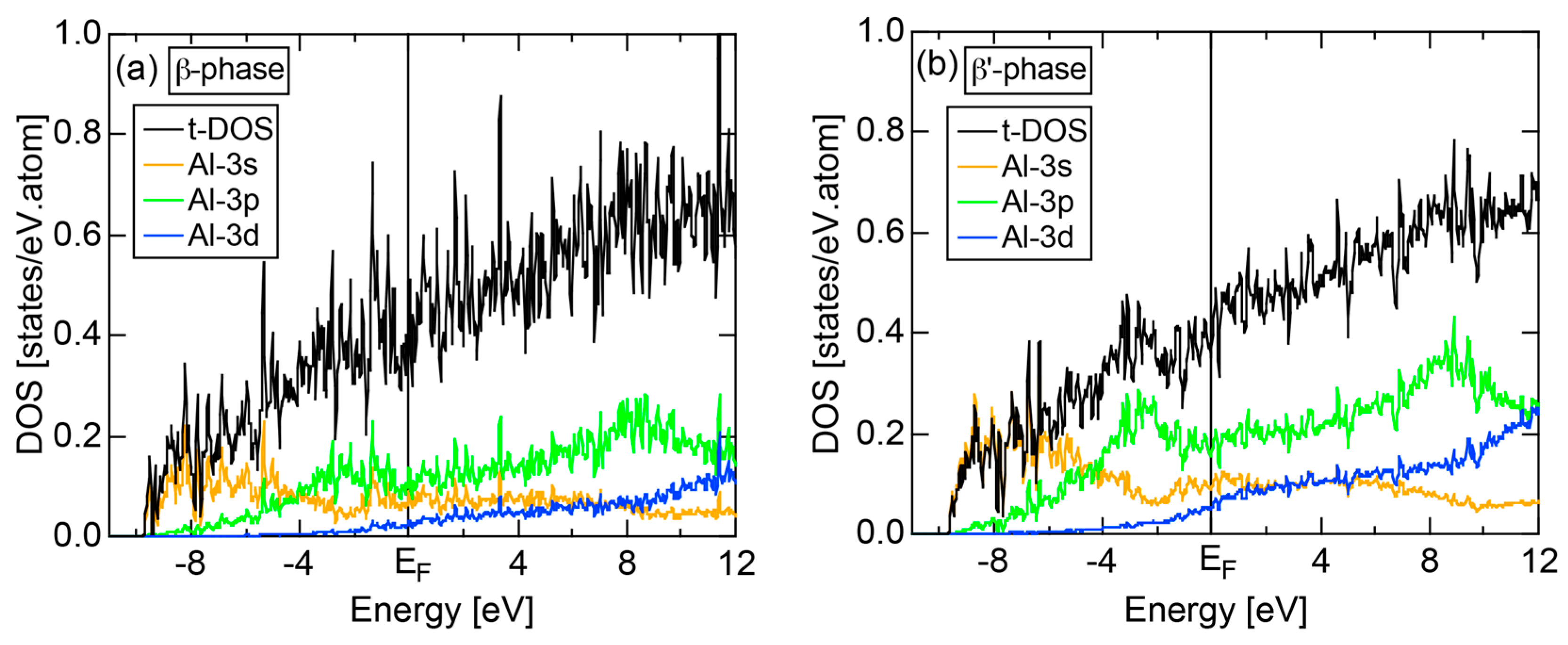
Figure 50.
(a) FLAPW-Fourier spectra at symmetry points Γ, L, X of the fcc Brillouin zone and at symmetry points of Γ, L, F of rhombohedral lattice; (b) and (c) Hume-Rothery plots for the β- and for β′-phase Al3Mg2 compounds, respectively [11]. Full- and dotted- blue curves in (a) indicate the total DOSs for the respective phases.
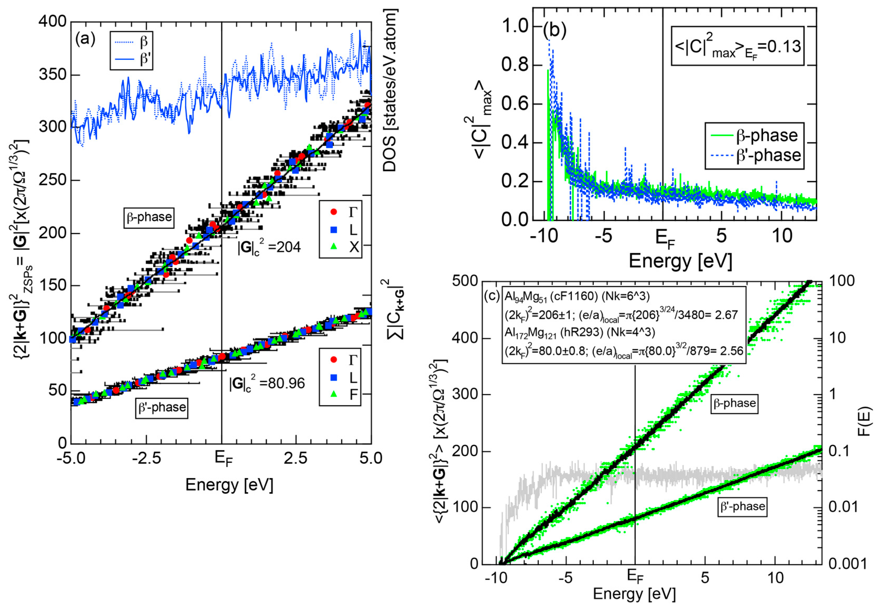
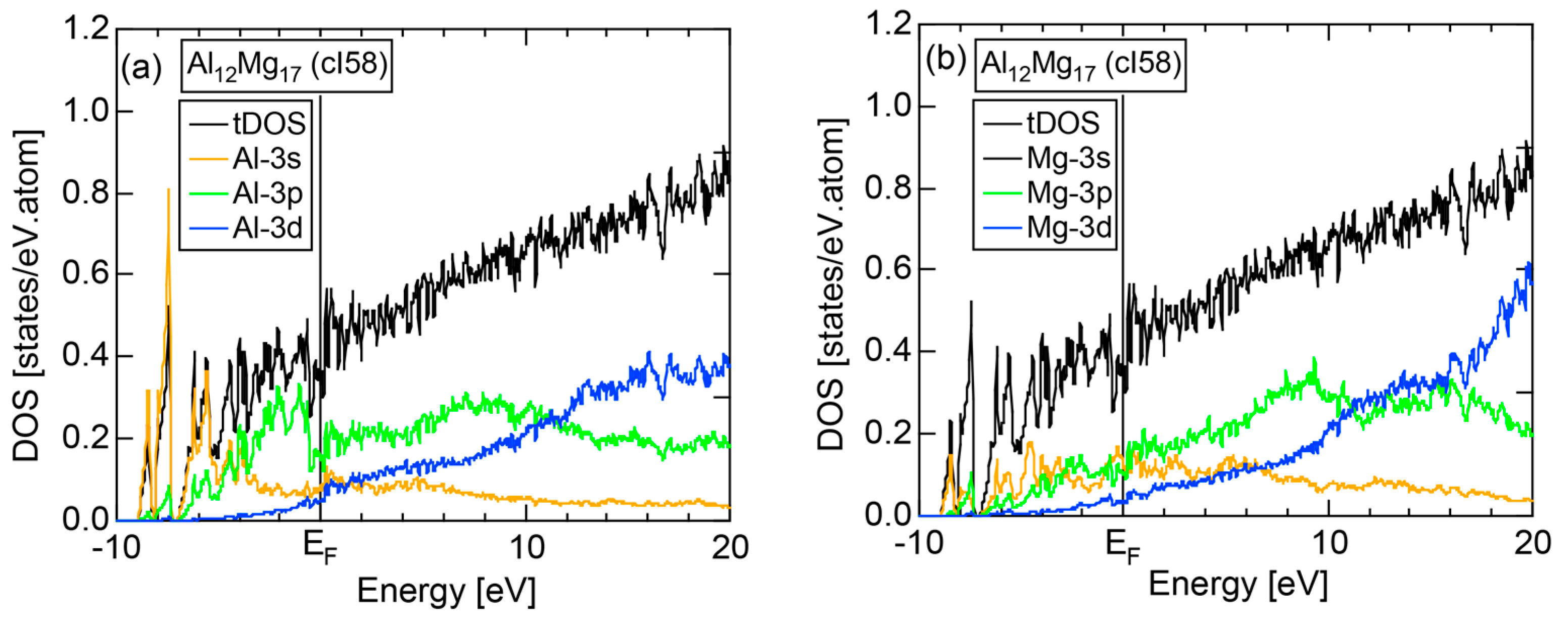
Figure 52.
(a) FLAPW-Fourier spectra at symmetry points Γ, N, H of the bcc Brillouin zone along with total-DOS; (b) and (c) Hume-Rothery plot for Al12Mg17 (cI58) [11,54].

Figure 53.
Composition dependence of e/a for compounds in Al-Mg alloy system [11].
Figure 53.
Composition dependence of e/a for compounds in Al-Mg alloy system [11].
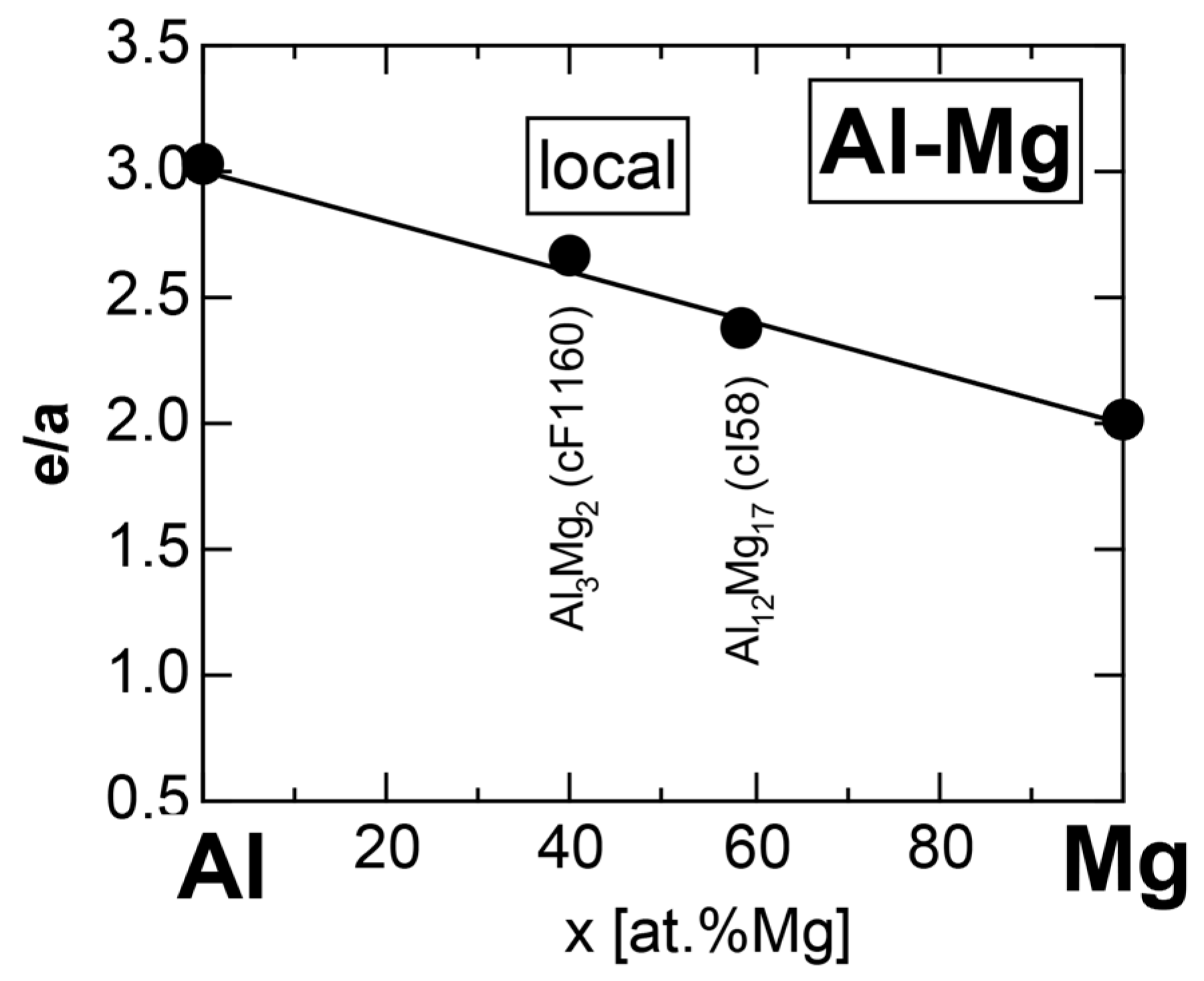
Figure 54.
Composition dependence of e/a for compounds in TM-Al (TM = Ti to Cu) alloy system [11]. The linear interpolation rule holds well.
Figure 54.
Composition dependence of e/a for compounds in TM-Al (TM = Ti to Cu) alloy system [11]. The linear interpolation rule holds well.
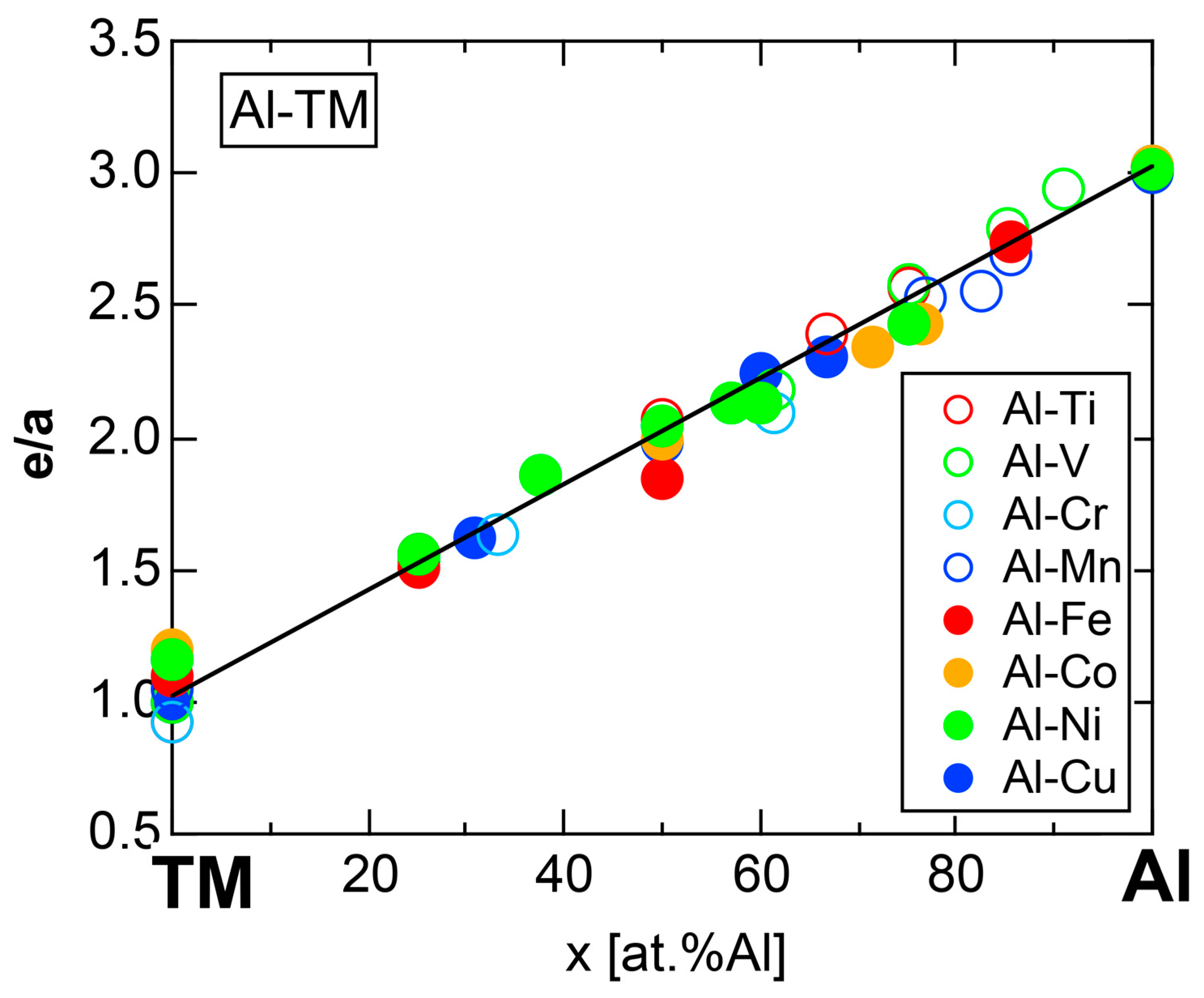
Figure 55.
e/uc versus diagram on a log-log scale for pseudogap-bearing Al-, Zn- and Cd-based compounds [11]. The NFE line (black) with a slope of 3/2 can be well fitted to all the compounds, regardless of the chemical bond-types involved. The critical reciprocal lattice vector is expressed in units of , where represents the effective lattice constant for any crystals. The interference condition given by Equation (20) has been referred to as the “3/2-power law”. No correlation is found between and e/a, which is plotted using the ordinate in the right-hand side.

Figure 56.
e/uc versus diagram on a log-log scale for RT-type 1/1-1/1-1/1 approximants in zone A and gamma-brasses in zone B [11]. They are classified into subgroups. The critical reciprocal lattice vector is expressed in units of , where is the lattice constant for cubic crystals. The 3/2-power law (red line) holds well, irrespective of subgroups involved.
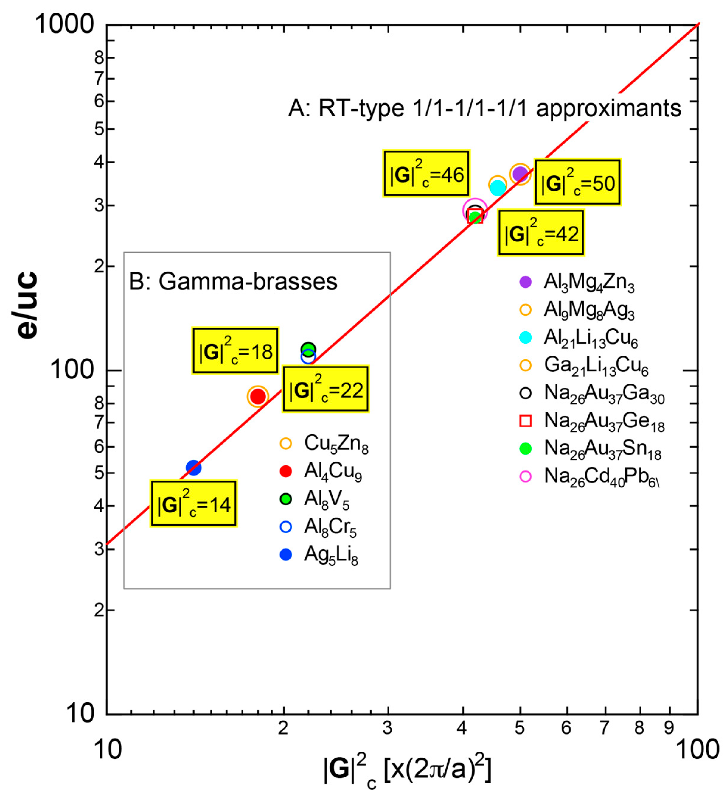
Figure 57.
Van Arkel-Ketelaar triangle map for Zintl compounds. It was constructed by inserting Allen’s electronegativity data (Table 2) into Equations (17) and (18) [11].

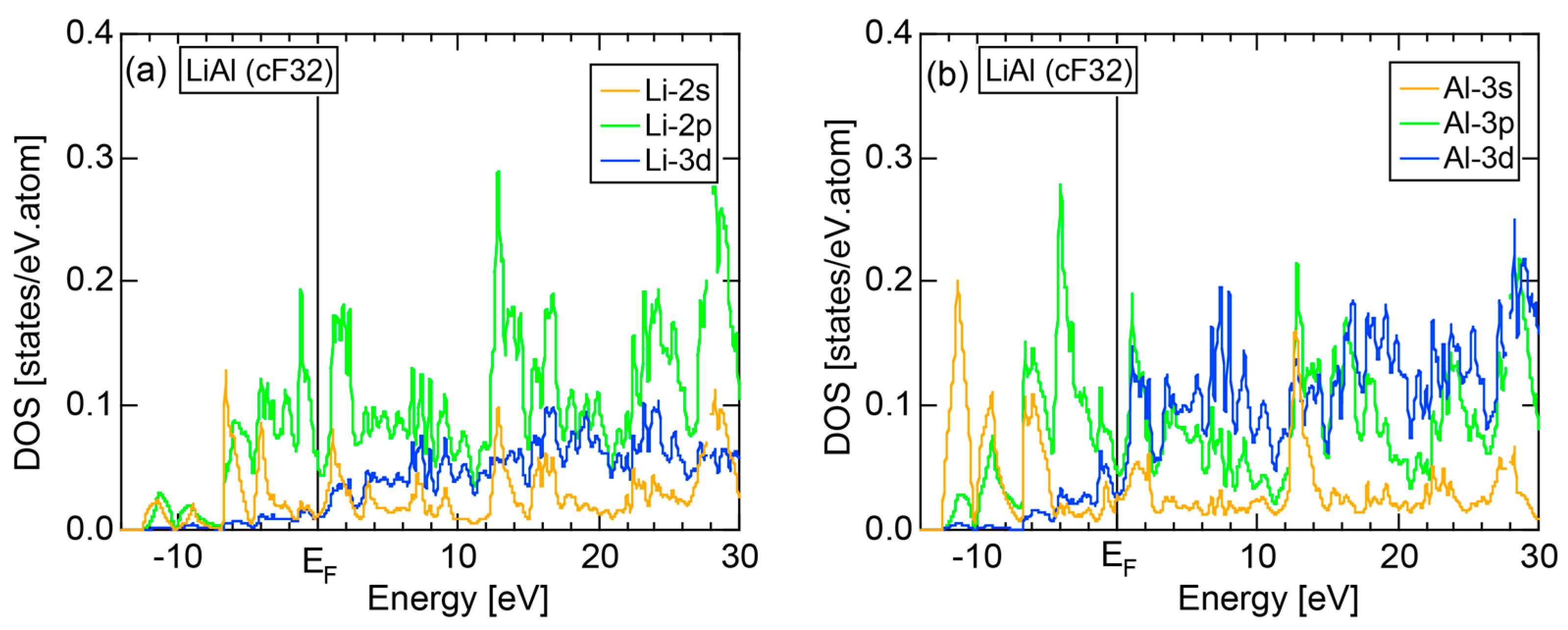
Figure 59.
(a) FLAPW-Fourier spectra at symmetry points Γ, L, X of the fcc Brillouin zone along with the total DOS; (b) and (c) Hume-Rothery plot for LiAL (cF32) [11,41]. See caption of Figure 19b for symbols in (c).
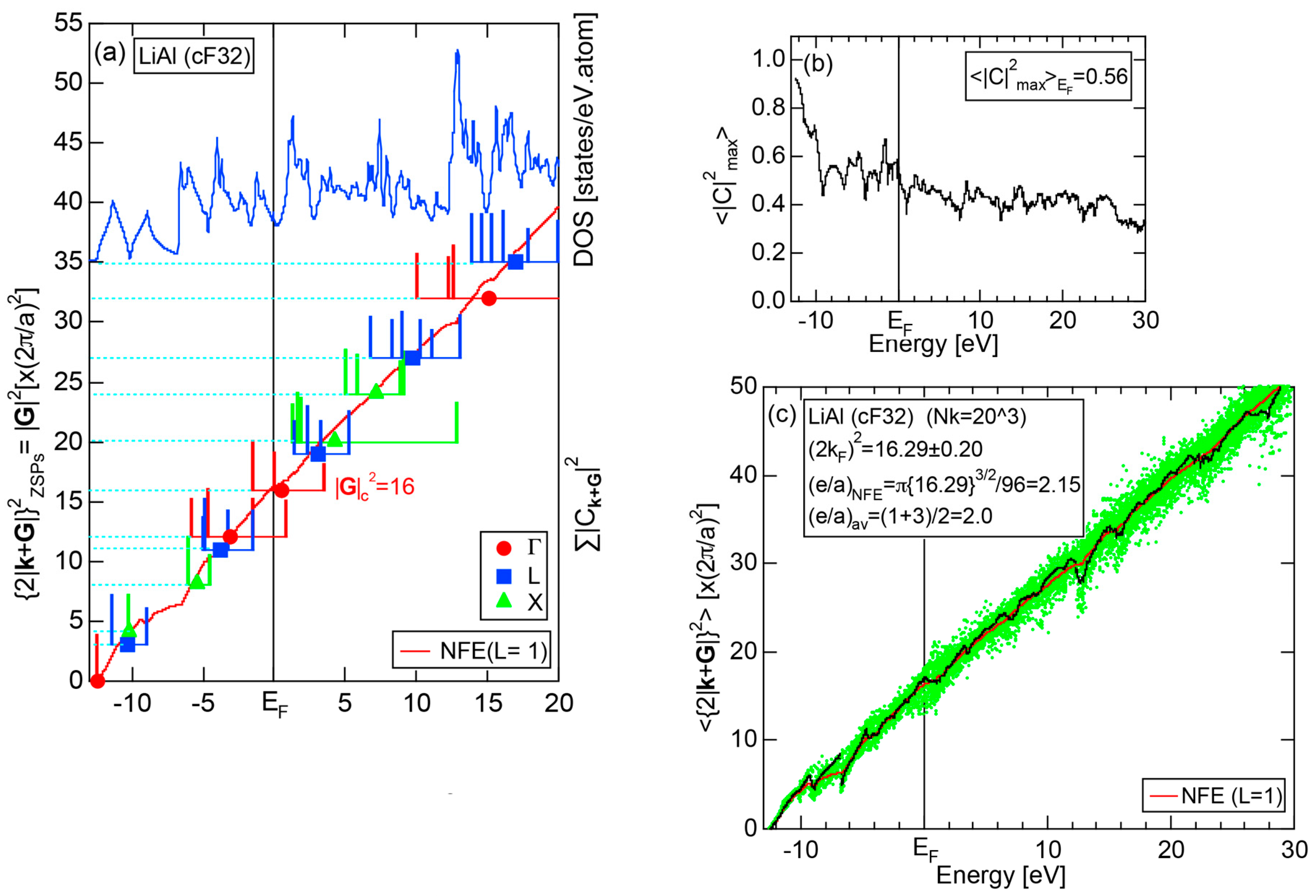
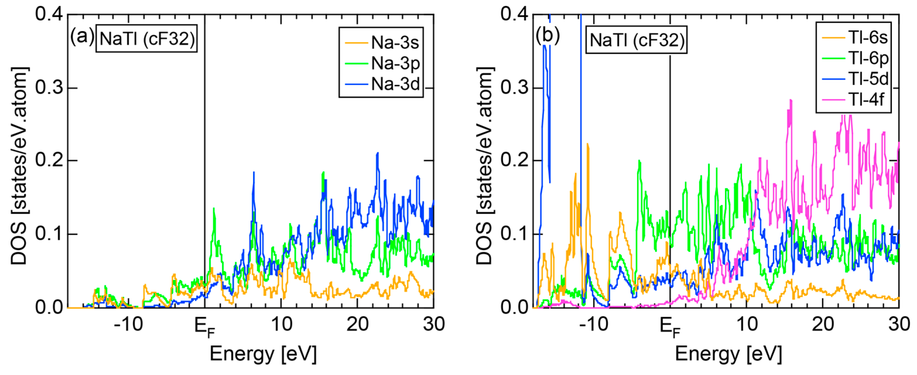
Figure 61.
(a) FLAPW-Fourier spectra at symmetry points Γ, L, X of the fcc Brillouin zone along with the total DOS; (b) and (c) Hume-Rothery plot for NaTl (cF32) [11,41]. See captions of Figure 19b for symbols in (c).

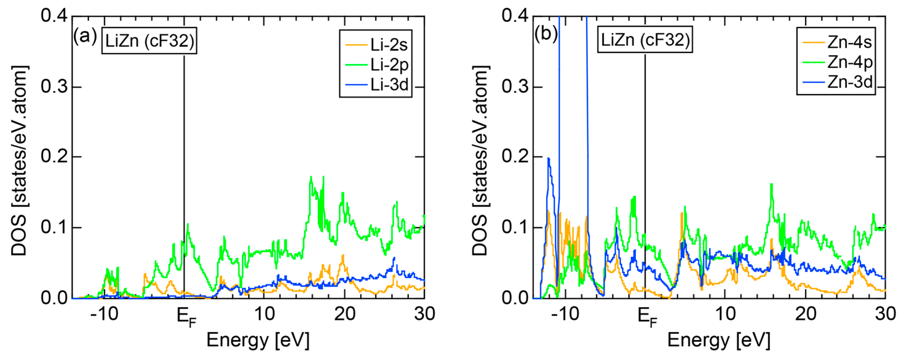
Figure 63.
(a) FLAPW-Fourier spectra at symmetry points Γ, L, X of the fcc Brillouin zone along with the total DOS; (b) and (c) Hume-Rothery plot for LiZn (cF32) [11,41]. See captions of Figure 19 (b) for symbols in (c).


Figure 65.
(a) FLAPW-Fourier spectra at symmetry points Γ, L, X of the fcc Brillouin zone along with the total DOS; (b) and (c) Hume-Rothery plot for LiCd (cF32) [11,41]. See captions of Figure 19 (b) for symbols in (c).
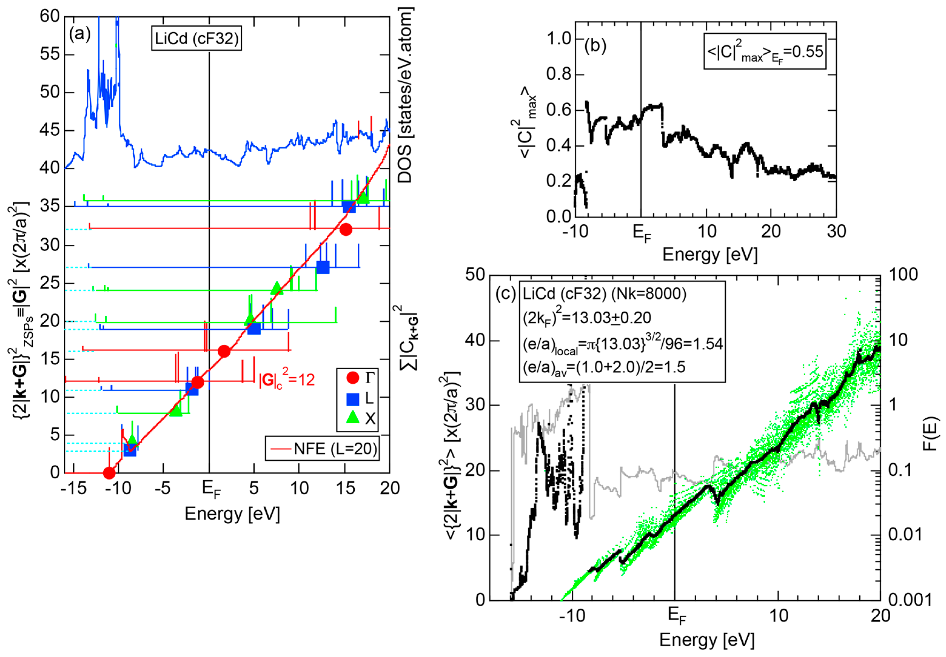
Figure 66.
Van Arkel-Ketelaar triangle map constructed by inserting the Allen electronegativity data (Table 2) into Equations (17) and (18) for equiatomic MP compounds (solid circles) and seven elements (open circles) in period 3 of the Periodic Table.
Figure 66.
Van Arkel-Ketelaar triangle map constructed by inserting the Allen electronegativity data (Table 2) into Equations (17) and (18) for equiatomic MP compounds (solid circles) and seven elements (open circles) in period 3 of the Periodic Table.
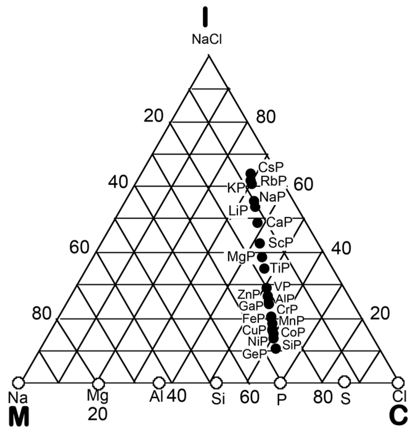
Figure 67.
(a) Si- and (b) P-pDOSs for SiP (oC48) and (c) Ge- and (d) P-pDOSs for GeP (tI4). The corresponding separation energies are also indicated.
Figure 67.
(a) Si- and (b) P-pDOSs for SiP (oC48) and (c) Ge- and (d) P-pDOSs for GeP (tI4). The corresponding separation energies are also indicated.

Figure 68.
(a) and (b) Hume-Rothery plot for SiP (oC48). The corresponding data for GeP (tI4) are in (c,d). See captions of Figure 19 (b) for symbols in (b) and (d).
Figure 68.
(a) and (b) Hume-Rothery plot for SiP (oC48). The corresponding data for GeP (tI4) are in (c,d). See captions of Figure 19 (b) for symbols in (b) and (d).
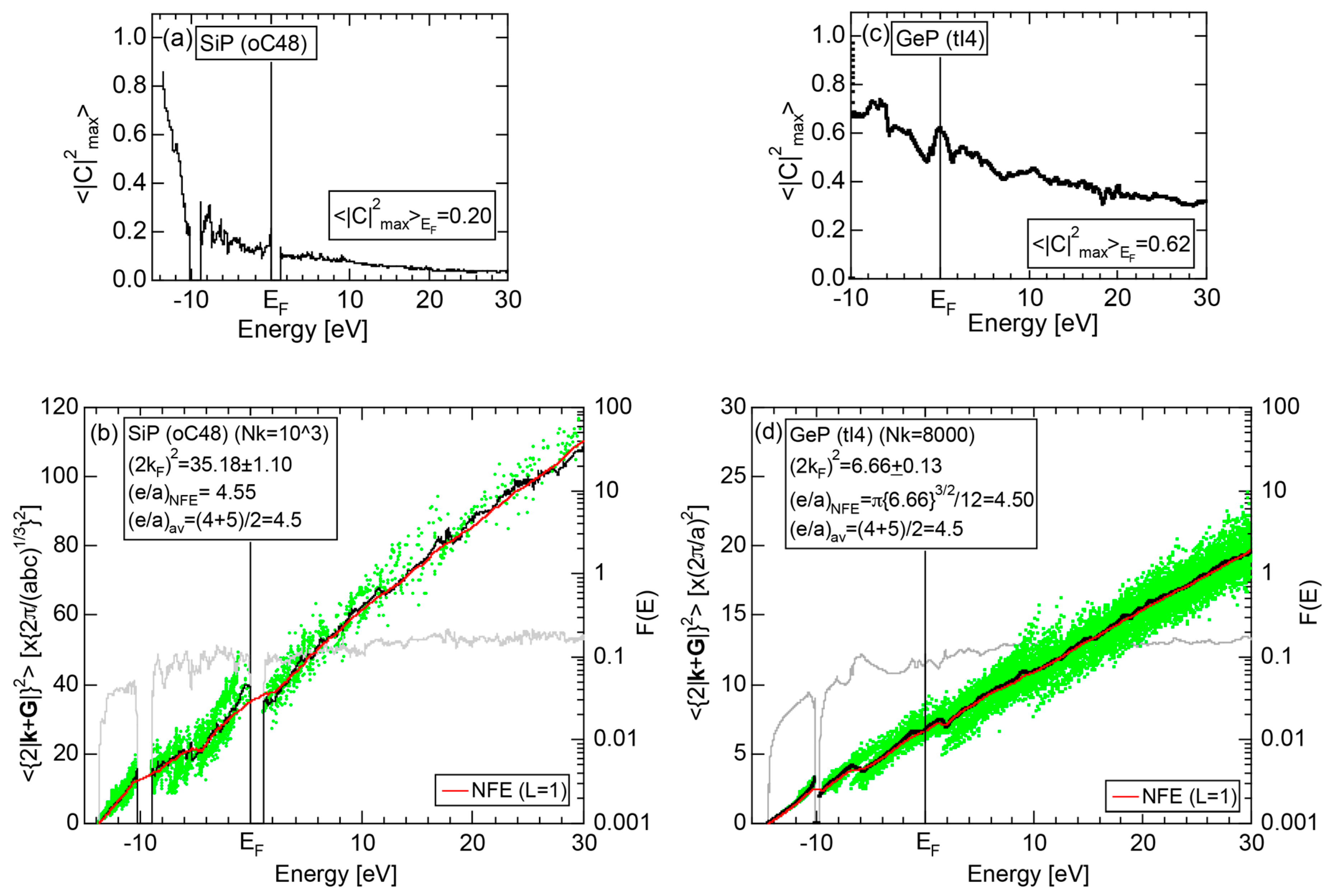
Figure 69.
Composition dependence of e/a for intermetallic compounds and pure elements in (a) Si-P and (b) Ge-P alloy systems. The NFE method is exclusively employed. The linear interpolation lines are drawn by connecting end points of pure elements in the respective alloy systems. Symbols in bracket refer to the Pearson symbol for elements and compounds [11].
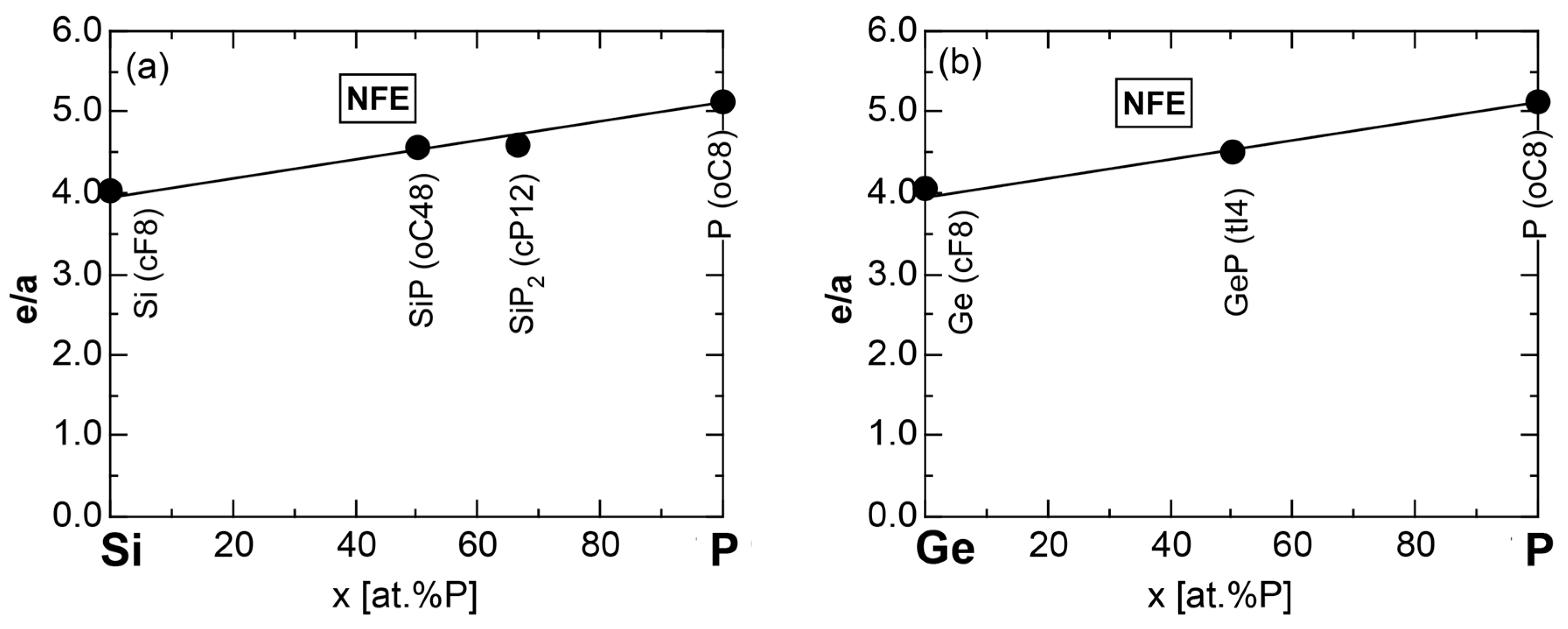
Figure 70.
(a) Sc- and (b) P-pDOSs for ScP (cF8). The corresponding separation energies are also indicated [11,12].

Figure 71.
(a) FLAPW-Fourier spectra at symmetry points Γ, L, and X of the fcc Brillouin zone along with the total DOS, (b) and (c) Hume-Rothery plot for ScP (cF8) [11,12]. See captions of Figure 34d for symbols in (c).
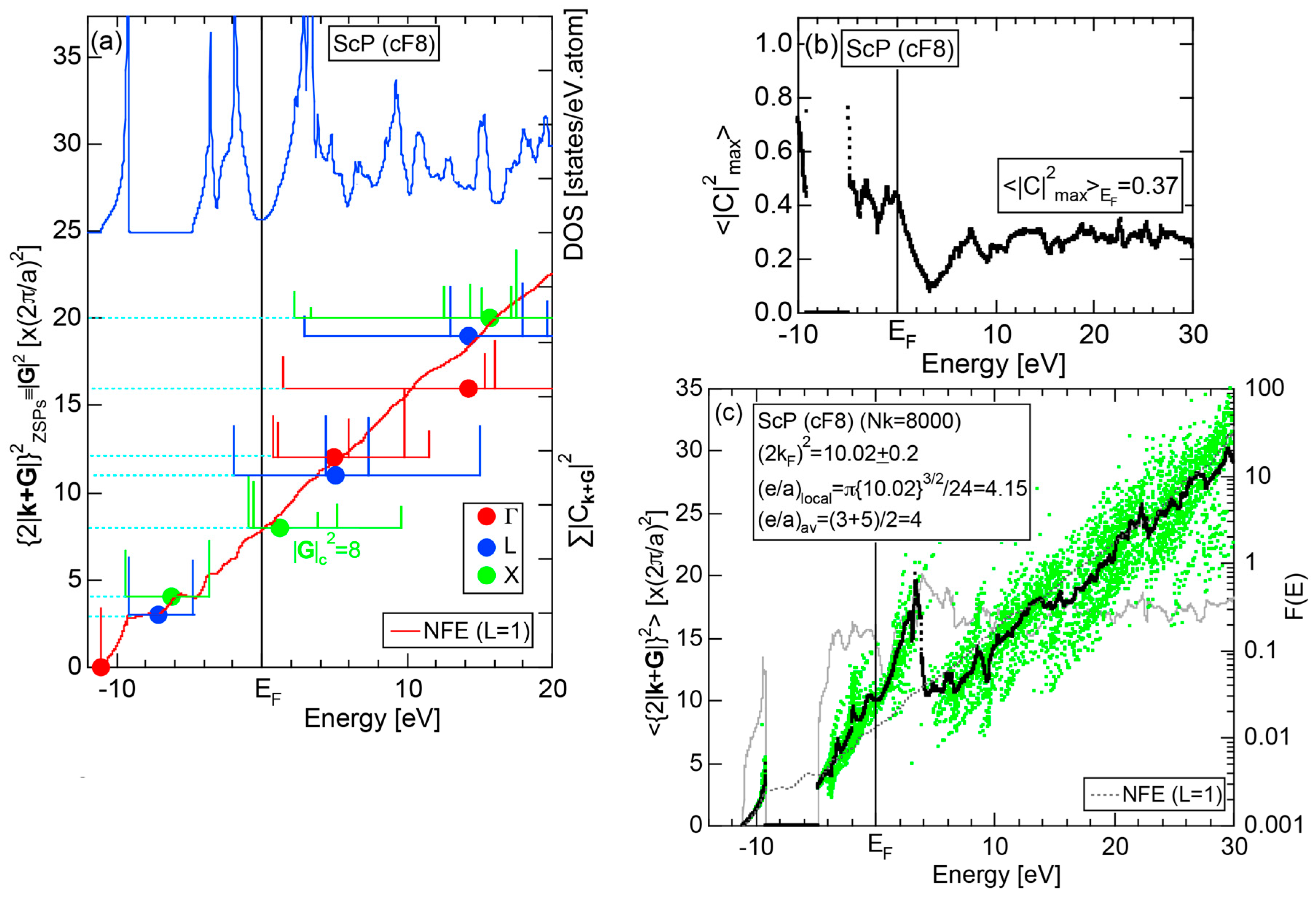
Figure 72.
(a) Y- and (b) P-pDOSs for YP (cF8).

Figure 73.
(a) FLAPW-Fourier spectra at symmetry points Γ, L, and X of the fcc Brillouin zone along with the total DOS, (b) and (c) Hume-Rothery plot for YP (cF8). See captions of Figure 19 (b) for symbols in (c).
Figure 73.
(a) FLAPW-Fourier spectra at symmetry points Γ, L, and X of the fcc Brillouin zone along with the total DOS, (b) and (c) Hume-Rothery plot for YP (cF8). See captions of Figure 19 (b) for symbols in (c).

Figure 74.
Composition dependence of e/a for intermetallic compounds and pure elements in (a) Sc-P and Y-P and (b) TM-P (TM=Ti to Cu) alloy systems [11]. The linear interpolation rule holds well in (a,b).
Figure 74.
Composition dependence of e/a for intermetallic compounds and pure elements in (a) Sc-P and Y-P and (b) TM-P (TM=Ti to Cu) alloy systems [11]. The linear interpolation rule holds well in (a,b).
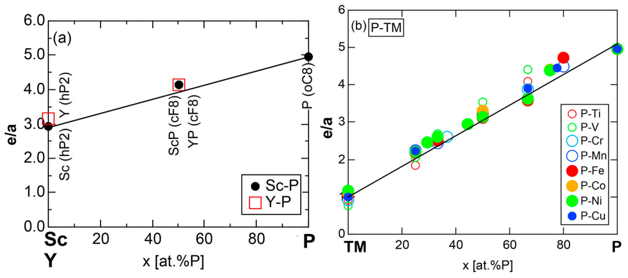
Figure 75.
(a) P-pDOSs and (b) Hume-Rothery plot for Mg3P2 (cI80) [11,12]. (c) P-pDOSs and (d) Hume-Rothery plot for CaP3 (aP8) [11,12]. See captions of Figure 19 (b) for symbols in (b) and (d).

Figure 76.
Composition dependence of e/a for intermetallic compounds and pure elements in (a) Zn-P and (b) Cu-P alloy systems [11]. The linear interpolation rule holds well in (a) and (b).
Figure 76.
Composition dependence of e/a for intermetallic compounds and pure elements in (a) Zn-P and (b) Cu-P alloy systems [11]. The linear interpolation rule holds well in (a) and (b).

Figure 77.
(a) Li- and (b) P-pDOSs, (c) and (d) Hume-Rothery plot for Li3P7 (oP40) [11,12]. The corresponding separation energies are also indicated in (a) and (b). See captions of Figure 19 (b) for symbols in (b) and (d) [11,12].

Figure 78.
(a) K-3d, P-3s, P-3p pDOSs and (b) Hume-Rothery plot for K2P3 (oF40) [11,12]. (c) Cs-5d, Cs-4f, P-3s, P-3p pDOSs and (d) Hume-Rothery plot for Cs2P3 (oF40) [11,12]. See captions of Figure 19 (b) for symbols in (b) and (d).

Figure 79.
P concentration dependence of e/a subjected to the NFE method for (a) Li−P; (b) Na−P; (c) K−P; (d) Rb−P; and (e) Cs−P alloy systems [11,12].

Figure 80.
(a) Co- and (b) P-pDOSs, (c) Hume-Rothery plot and (d) FLAPW-Fourier spectra at symmetry points Γ, N, and H of the bcc Brillouin zone along with the total DOS (blue), Co-4p (green) and P-3p (yellow) for CoP3 (cI32) [11,12]. See captions of Figure 19 (b) for symbols in (c).

Figure 81.
(a) Cr- and (b) P-pDOSs for CrP (oP8) and (c) Mn- and (d) P-pDOSs for MnP (oP8) [11]. The corresponding separation energies are also indicated in (a) to (d).
Figure 81.
(a) Cr- and (b) P-pDOSs for CrP (oP8) and (c) Mn- and (d) P-pDOSs for MnP (oP8) [11]. The corresponding separation energies are also indicated in (a) to (d).

Figure 82.
(a) Fe- and (b) P-pDOSs for FeP (oP8) and (c) Co- and (d) P-pDOSs for CoP (tI32) [11].
Figure 82.
(a) Fe- and (b) P-pDOSs for FeP (oP8) and (c) Co- and (d) P-pDOSs for CoP (tI32) [11].

Figure 83.
(a) Hume-Rothery plots and the NFE (L = 1) curves and (b) for TMP (TM = Cr, Mn, Fe and Co) (oP8) compounds.
Figure 83.
(a) Hume-Rothery plots and the NFE (L = 1) curves and (b) for TMP (TM = Cr, Mn, Fe and Co) (oP8) compounds.

Figure 84.
(a) Cr- and (b) P-pDOSs for Cr3P (tI32) and (c) Mn- and (d) P-pDOSs for Mn3P (tI32) [11].
Figure 84.
(a) Cr- and (b) P-pDOSs for Cr3P (tI32) and (c) Mn- and (d) P-pDOSs for Mn3P (tI32) [11].

Figure 85.
(a) Fe- and (b) P-pDOSs for Fe3P (tI32) and (c) Ni- and P-pDOSs for Ni3P (tI32) [11].
Figure 85.
(a) Fe- and (b) P-pDOSs for Fe3P (tI32) and (c) Ni- and P-pDOSs for Ni3P (tI32) [11].

Figure 86.
(a) Hume-Rothery plots and (b) the NFE (L = 1) curves for TM3P (TM = Cr, Mn, Fe, and Ni) (tI32) compounds [12].
Figure 86.
(a) Hume-Rothery plots and (b) the NFE (L = 1) curves for TM3P (TM = Cr, Mn, Fe, and Ni) (tI32) compounds [12].

Figure 87.
FLAPW−Fourier spectra at symmetry points Γ, N, X, Z, and P of the bct Brillouin zone for (a) Cr3P, (b) Mn3P, (c) Fe3P, and (d) Ni3P (tI32) [12]. A red arrow indicates the minimum in the partial DOSs. The energy dependence of the Fourier coefficients, , is plotted only for Cr3P. The CG energy is plotted with different color circles.

Figure 88.
e/uc versus diagram on a log-log scale for pseudogap- or true gap-bearing Phosphorus compounds. The NFE line with a slope of 3/2 (red) can be universally drawn for all compounds, regardless of the chemical bond-types involved. The data for host metal P is marked with open circle. The critical reciprocal lattice vector is expressed in units of , where represents the effective lattice constant for any crystals. Note that the interference condition is given by Equation (20). This has been referred to as the “3/2-power law”.

Figure 89.
(a) Ca-partial DOSs, (b) and (c) Hume-Rothery plot for Ca (cF4) [11,15,16,37]. See captions of Figure 19 (b) for symbols in (c). Two distinct e/a values are obtained for Ca (cF4), depending on either the local reading or the NFE method.

Figure 90.
(a) Sr-partial DOSs, (b) and (c) Hume-Rothery plot for Sr (cF4) [11,15,16,37]. See captions of Figure 19 (b) for symbols in (c). The same value of e/a is obtained for Sr (cF4), regardless of whether the local reading or the NFE method is employed.
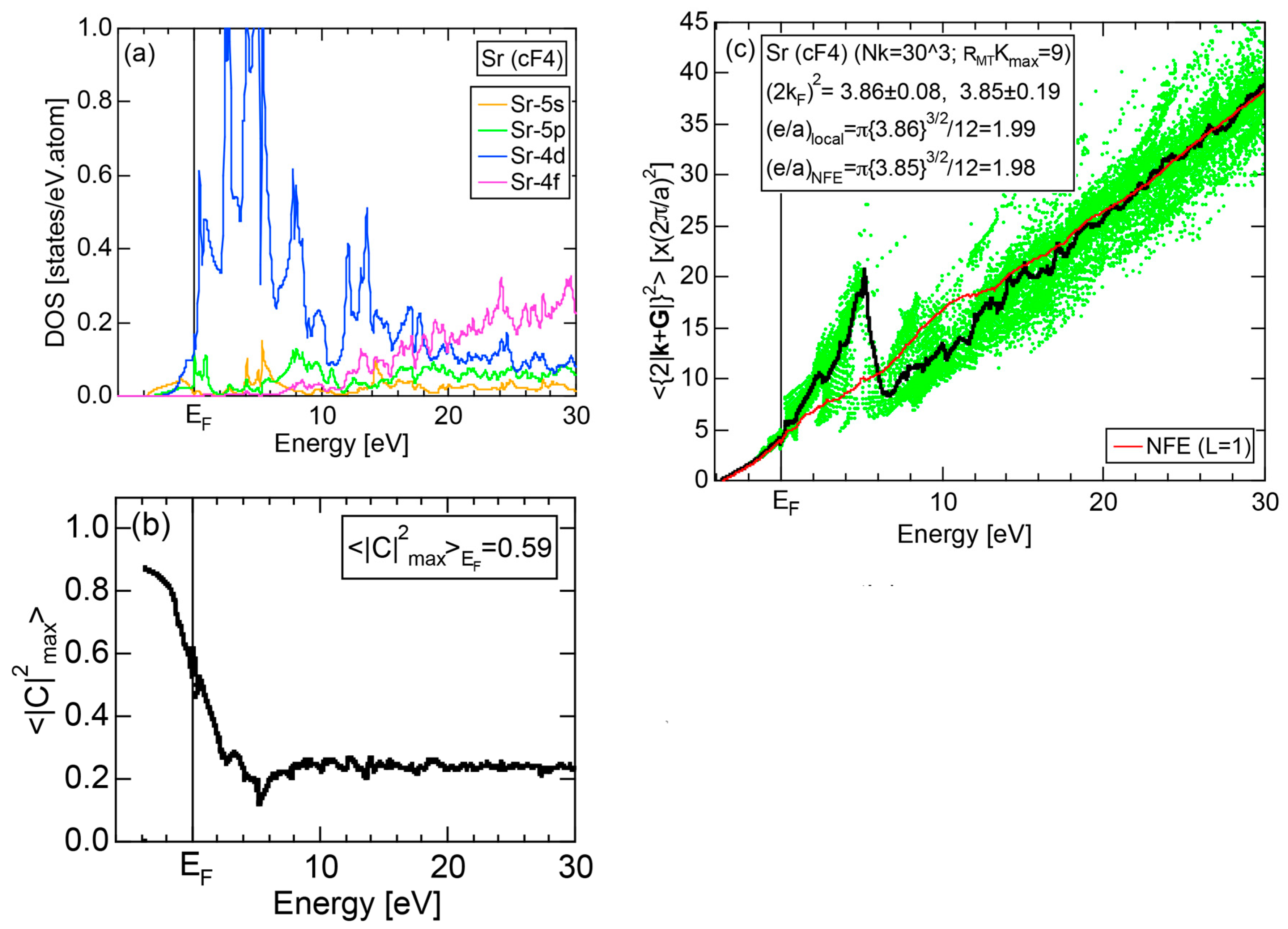
Figure 91.
(a) Ba-partial DOSs, (b) and (c) Hume-Rothery plot for Ba (cI2) [11,15,16,37]. See captions of Figure 19 (b) for symbols in (c). The value of e/a determined from the NFE curve (L = 1) was exclusively employed for Ba (cI2), regardless of partner elements involved.
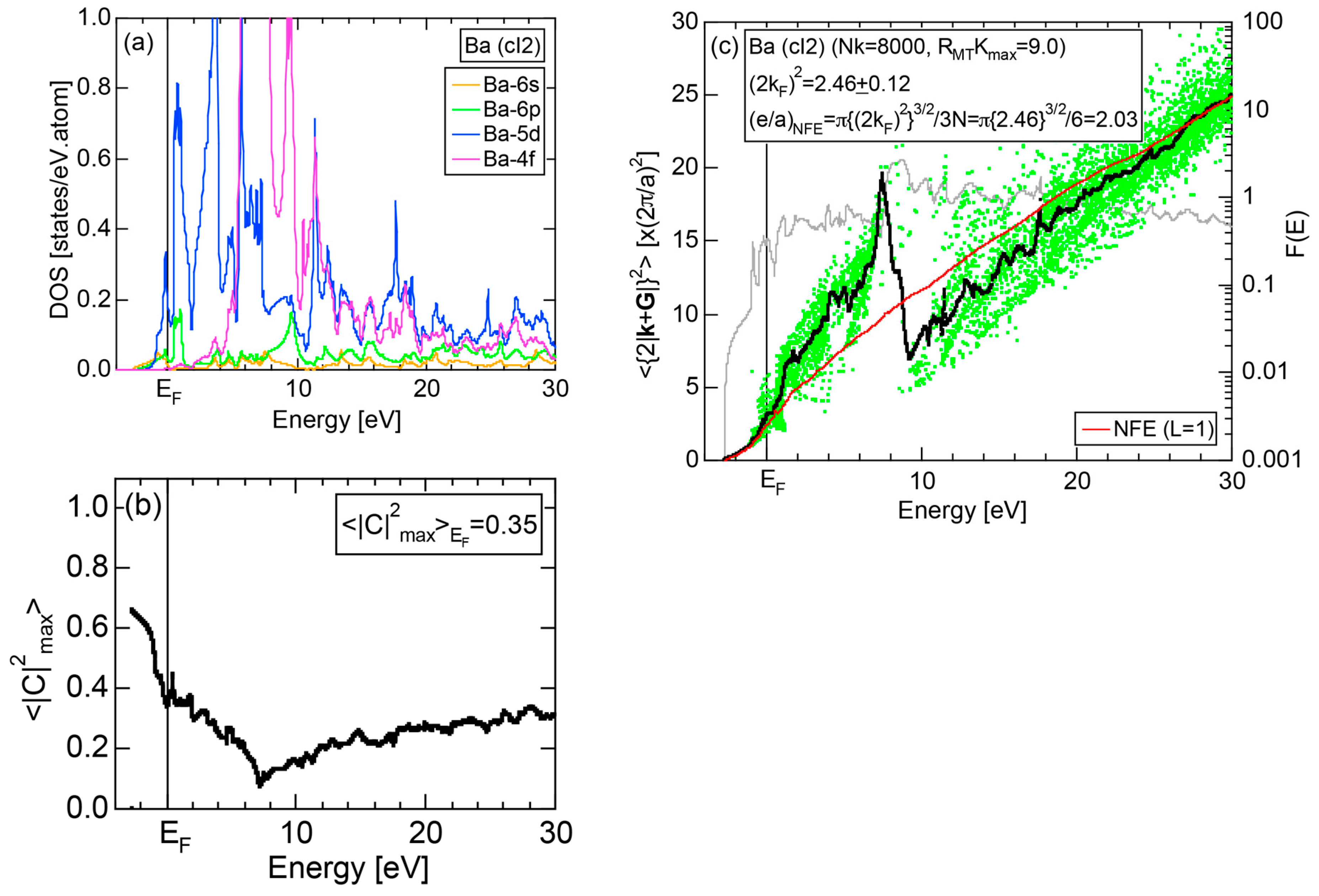
Figure 92.
(a) Sc-partial DOSs, (b) and (c) Hume-Rothery plot for Sc (hP2) [11,15,16,37]. See captions of Figure 19 (b) for symbols in (c). Two distinct e/a values are obtained for Sc (hP2), depending on either the local reading or the NFE method.
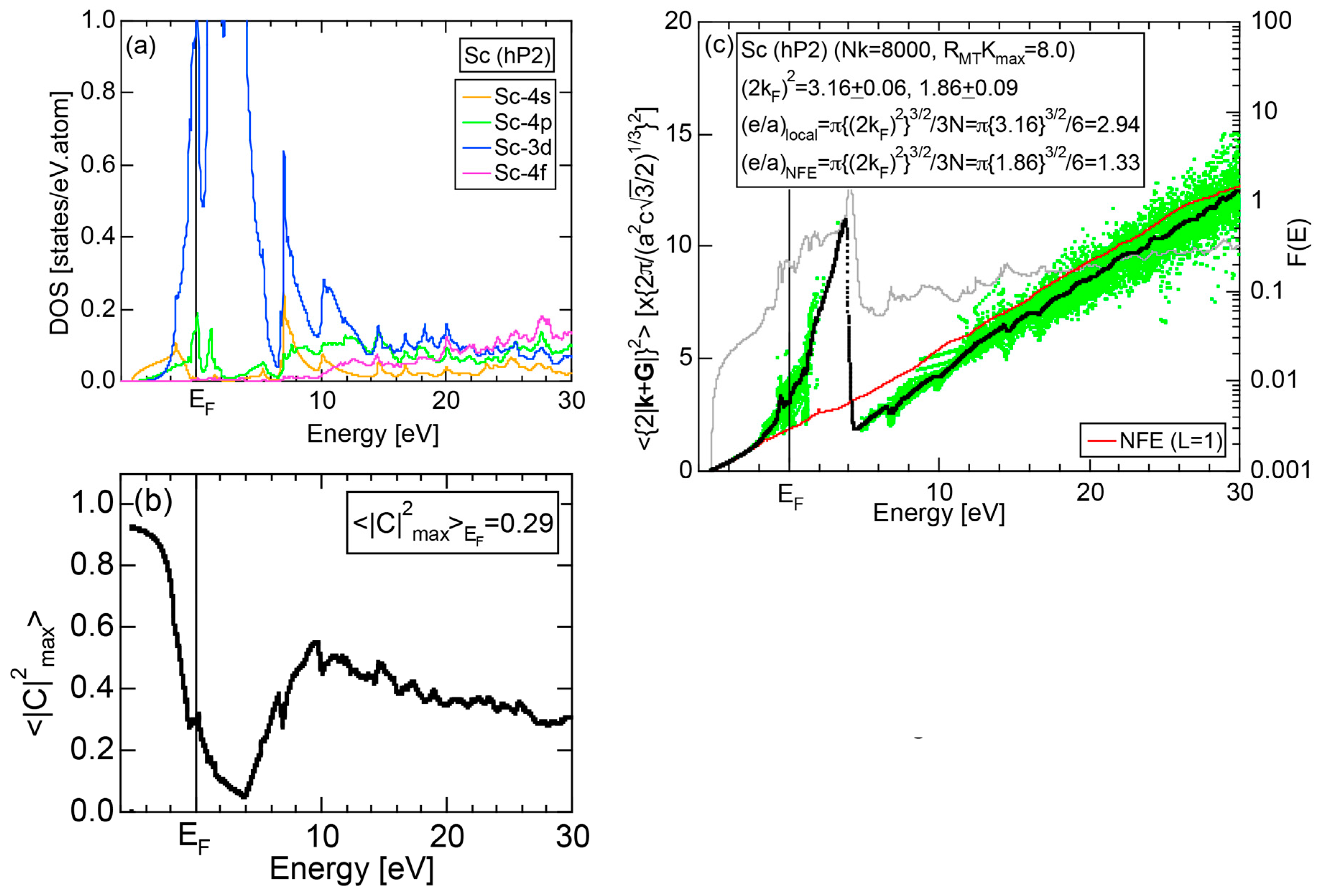
Figure 93.
(a) Y-partial DOSs, (b) and (c) Hume-Rothery plot for Y (hP2) [11,15,16,37]. See captions of Figure 19 (b) for symbols in (c). Two distinct e/a values are obtained for Y (hP2), depending on either the local reading or the NFE method.
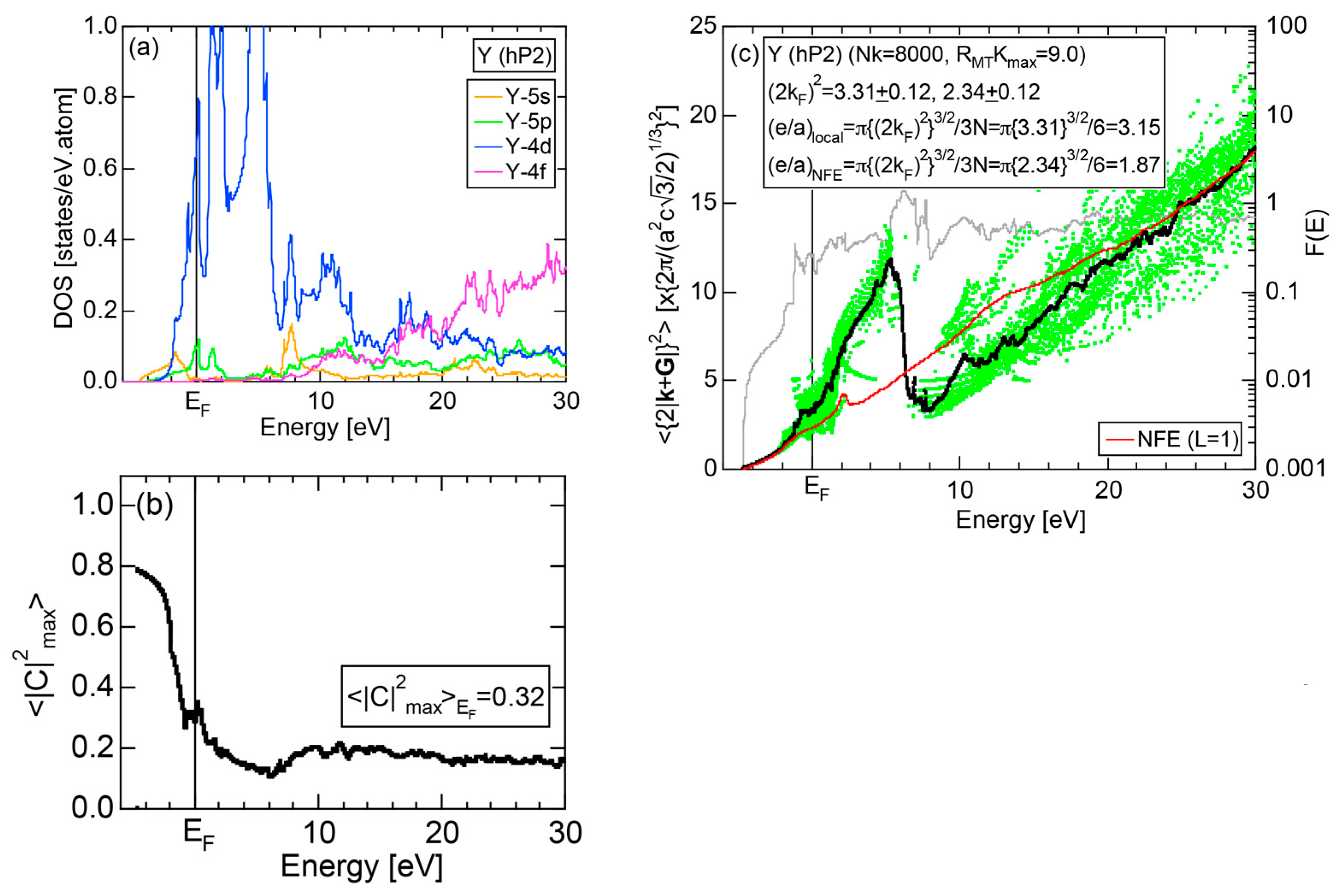
Figure 94.
(a) La-partial DOSs, (b) and (c) Hume-Rothery plot for La (hP4) [11,15,16,37]. See captions to Figure 19 (b) for symbols in (c). The value of e/a determined from the NFE curve (L = 1) was exclusively employed for La (hP4), regardless of partner elements involved.
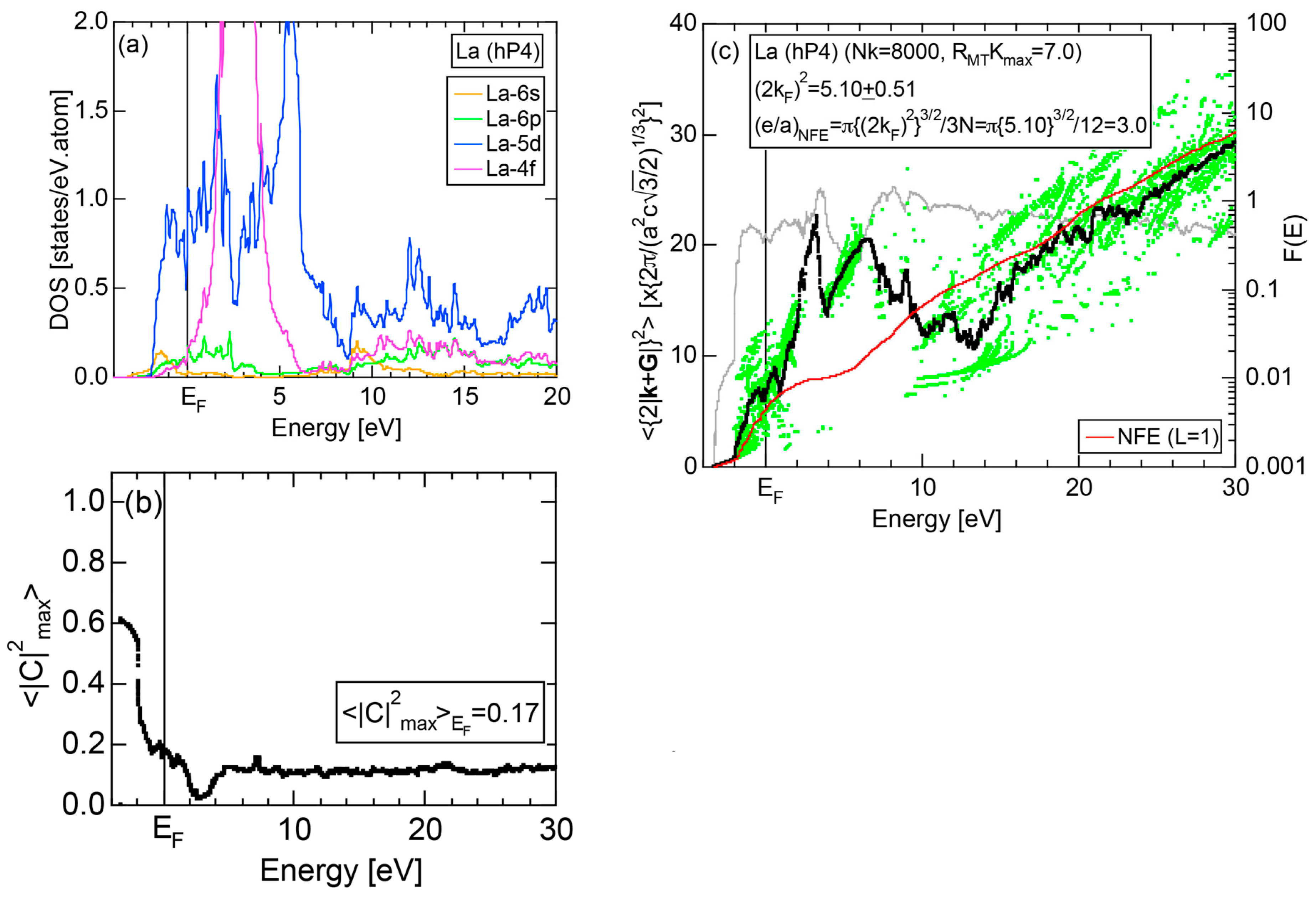
Figure 95.
Composition dependence of e/a for intermetallic compounds and pure elements in (a) Ca–M (M = Zn, Cd, Al), (b) Sr–M (M=Zn, Al), (c) Sc-M (M = Ag, Zn, Al) and Y-M (M = Ag, Zn, Cd, Al) alloy systems [37]. The local reading method is exclusively employed. The linear interpolation lines are drawn by connecting end points of pure elements in the respective alloy systems. Symbols in bracket refer to the Pearson symbol for elements and compounds.

Figure 96.
Composition dependence of e/a for intermetallic compounds and pure elements in (a) Ba–M (M = Ag, Zn, Cd, Al, Ga) and (b) La–M (M = Cu, Ag, Mg, Zn, Cd, Al, Ga, In) alloy systems [37]. The NFE method is employed for elements Ba, La and all the compounds but the local reading method for elements located at 100 at.%M. The linear interpolation lines are drawn by connecting end points of pure elements in the respective alloy systems. Symbols in bracket refer to the Pearson symbol for elements and compounds.

Figure 97.
Composition dependence of e/a for intermetallic compounds and pure elements in (a) Ca–TM (TM = Ni, Pd), (b) Sr–TM (TM=Rh, Pd, Ir, Pt) and (c) Ba-TM (TM=Pd, Pt) alloy systems [37]. The NFE method is exclusively employed. The linear interpolation lines are drawn by connecting end points of pure elements in the respective alloy systems. Symbols in bracket refer to the Pearson symbol for elements and compounds.

Figure 98.
Composition dependence of e/a for intermetallic compounds and pure elements in (a) Sc–TM (TM = Co, Ni, Ir), (b) Y–TM (TM = Mn, Fe, Co, Pd, Re, Pt) and (c) La-TM (TM = Co, Ni, Ru, Rh, Pd, Pt) alloy systems [37]. The NFE method is exclusively employed. The linear interpolation lines are drawn by connecting end points of pure elements in the respective alloy systems. Symbols in bracket refer to the Pearson symbol for elements and compounds.

Figure 99.
Composition dependence of e/a for intermetallic compounds and pure elements in TM1–TM2 (TM1 = Ti, Mn, Zr, Ta) and (TM2 = Cr, Fe, Co, Pt) alloy systems [37]. The NFE method is exclusively employed. The linear interpolation lines are drawn by connecting end points of pure elements in the respective alloy systems. Symbols in bracket refer to the Pearson symbol for elements and compounds.

Figure 100.
van Arkel-Ketelaar triangle map constructed by inserting the Allen electronegativity (see Table 2) into Equations (17) and (18) for 50 equiatomic compounds AB. This may be used as a guide to roughly envisage bond-styles of Laves compounds AB2.
Figure 100.
van Arkel-Ketelaar triangle map constructed by inserting the Allen electronegativity (see Table 2) into Equations (17) and (18) for 50 equiatomic compounds AB. This may be used as a guide to roughly envisage bond-styles of Laves compounds AB2.
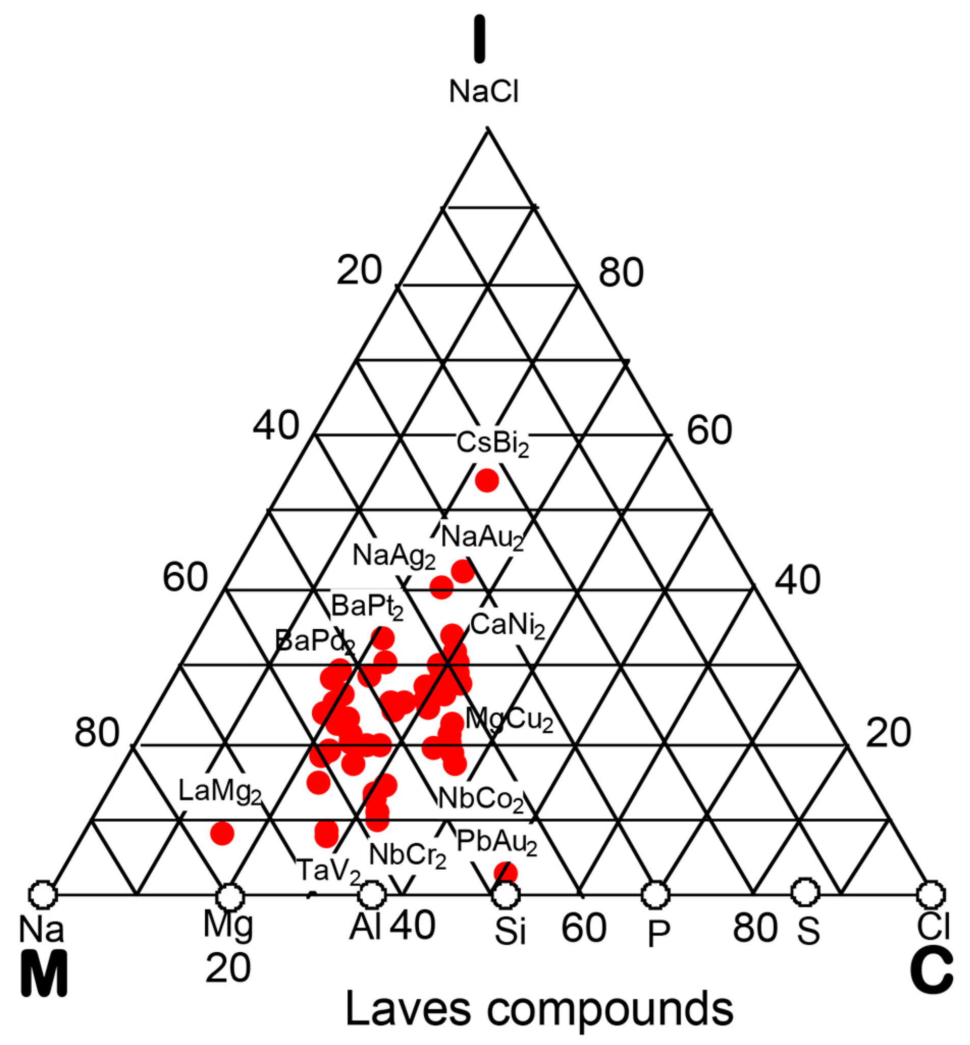
Figure 101.
(a) Co- and (b) Y-partial DOSs for Laves compound YCo2 (cF24) [37].
Figure 101.
(a) Co- and (b) Y-partial DOSs for Laves compound YCo2 (cF24) [37].
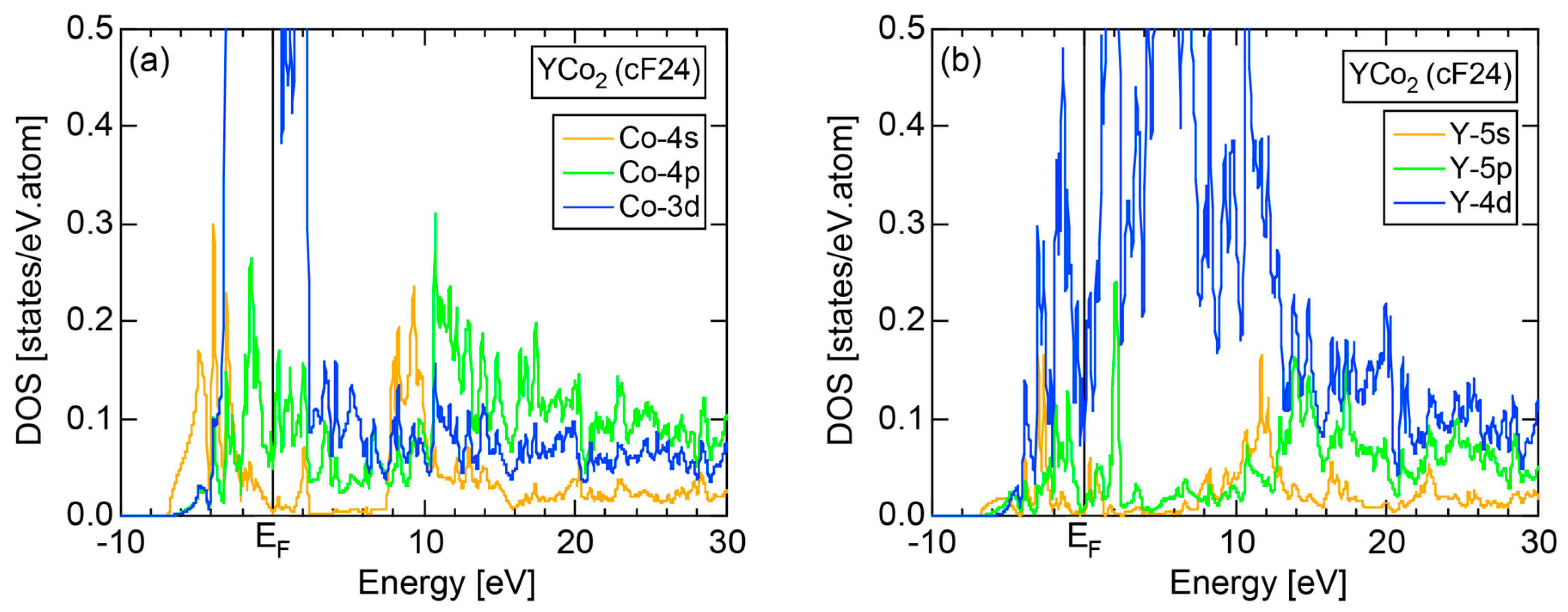
Figure 102.
(a) , (b) Hume-Rothery plot and FLAPW-Fourier spectra for Laves compound YCo2 (cF24) [37]. See captions to Figure 19 (b) for symbols in (c). Symbols in (c) refer to the total DOS (blue), Co-4p (purple) and Y-5p (green) partial DOSs and the center of gravity energy for -specified plane wave spectra at (red circle), L (blue circle) and X (green circle) symmetry points of the fcc-Brillouin zone, the NFE (L = 2) curve (red curve).

Figure 103.
-dependence of e/a for Laves compounds (cF24) [37]. Three integers in the curly bracket indicate Miller indices of the set of lattice planes corresponding to .
Figure 103.
-dependence of e/a for Laves compounds (cF24) [37]. Three integers in the curly bracket indicate Miller indices of the set of lattice planes corresponding to .
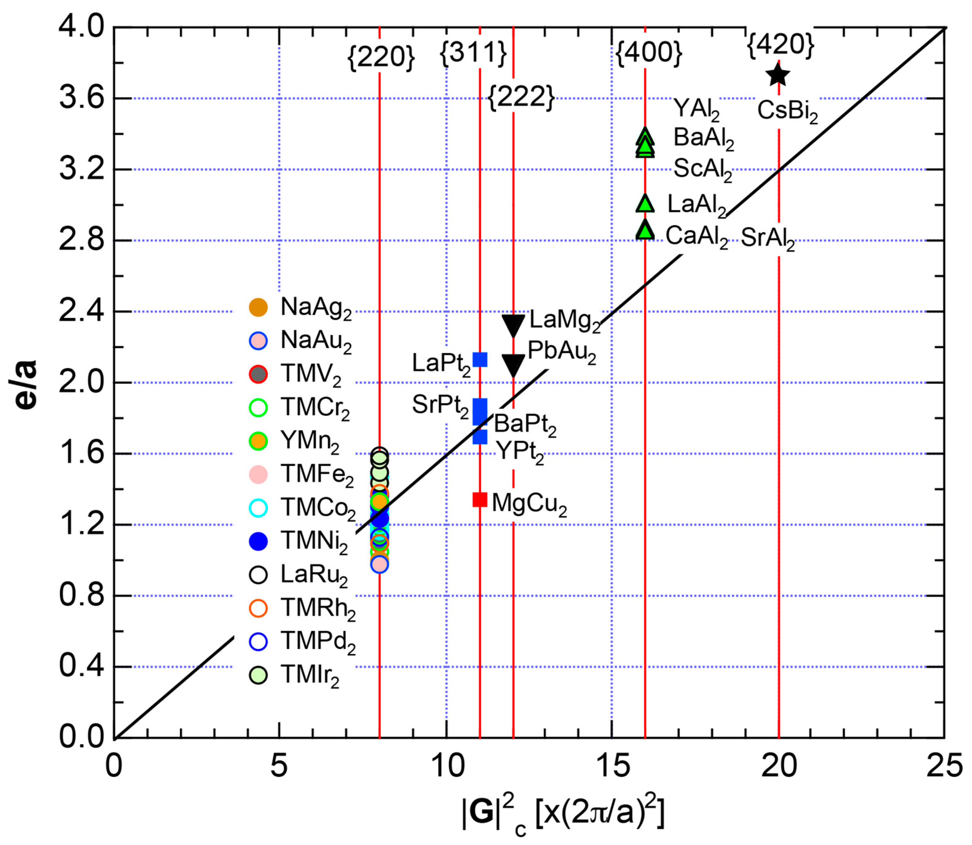
Figure 104.
e/a for Laves compounds (cF24) characterized by = 8 [37].
Figure 104.
e/a for Laves compounds (cF24) characterized by = 8 [37].
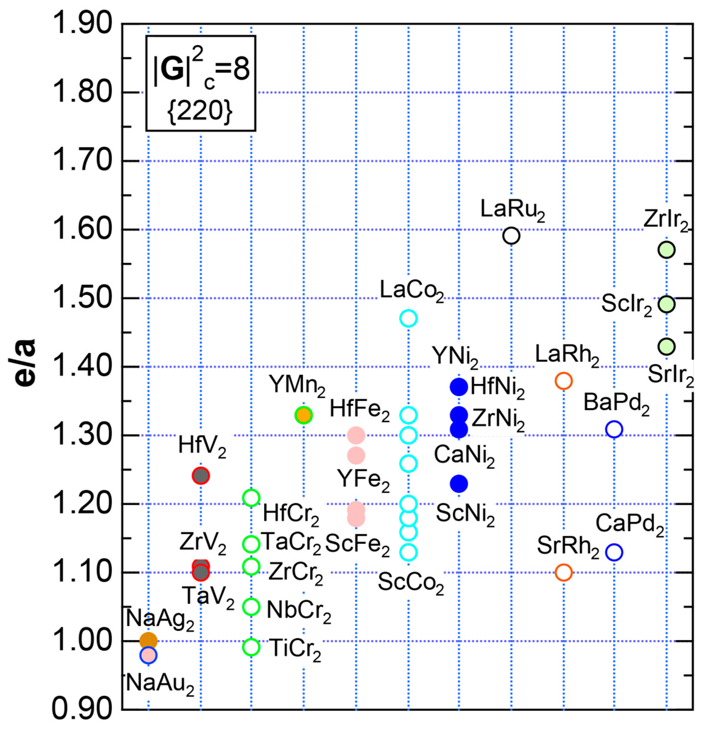
Figure 105.
versus for Laves compounds studied in [37]. Yellow zone is bounded by the two lines, one higher and the other lower by 20% relative to the line = .
Figure 105.
versus for Laves compounds studied in [37]. Yellow zone is bounded by the two lines, one higher and the other lower by 20% relative to the line = .
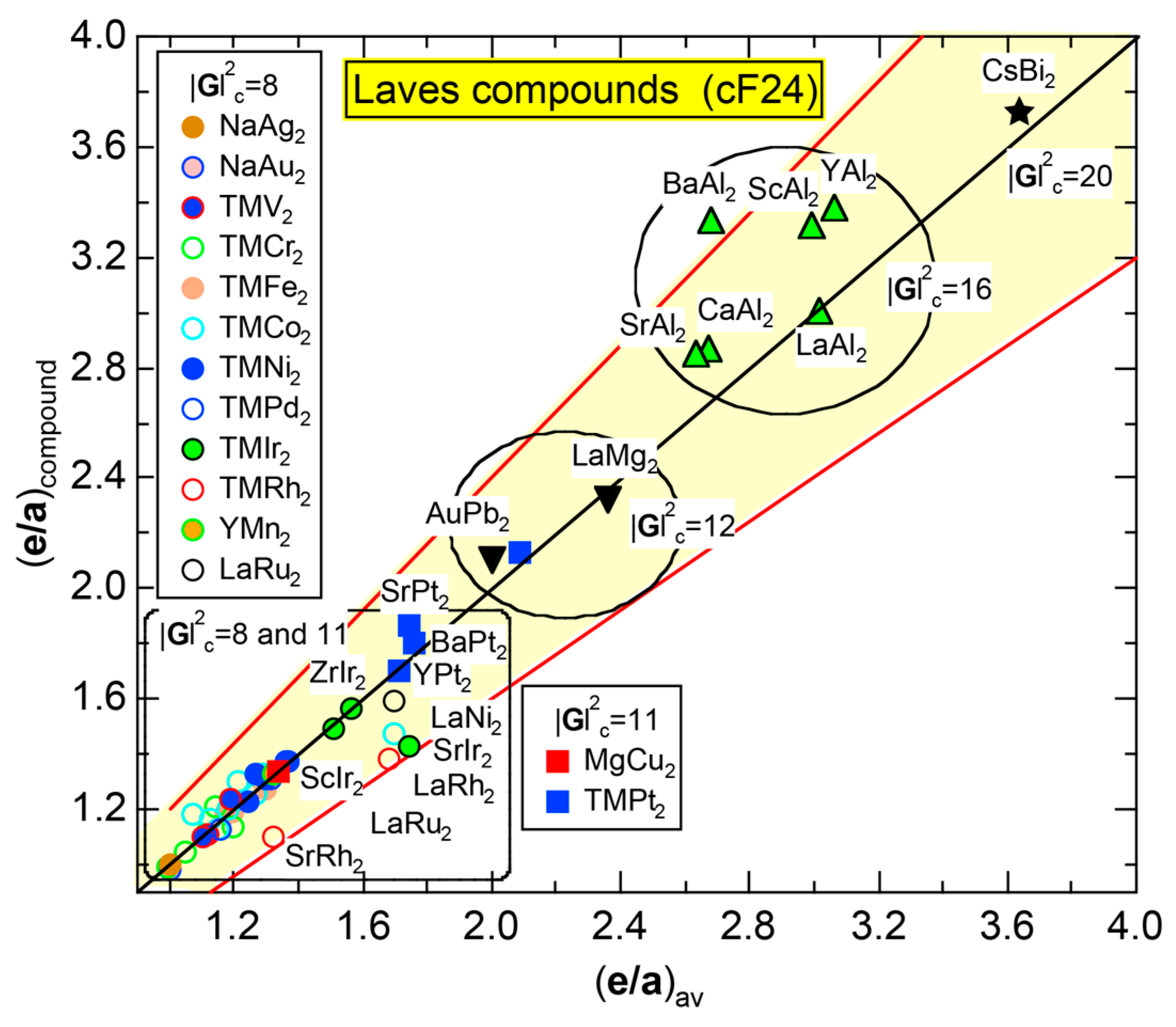
Figure 106.
(a) Ga- and (b) As-pDOSs, (c) Hume-Rothery plot and (d) FLAPW-Fourier spectra at symmetry points Γ, L, and X of the fcc Brillouin zone along with the total DOS for GaAs (cF8). See captions to Figure 19 (b) for symbols in (c) [37].

Figure 107.
(e/a)compound versus (e/a)av for Al-TM () and P-TM () compounds studied in the present work, where TM covers from Sc to Cu in Period 4 in the Periodic Table. The data from Figure 54 and Figure 74 are combined. The data for pure elements marked with open circles are located on the line (e/a)compound = (e/a)av. Numerical data in Table 1 are rounded off to the nearest integer or valence for simple elements but are used as they are for TM elements. The yellow gradation area is centered at e/a = 4.0.
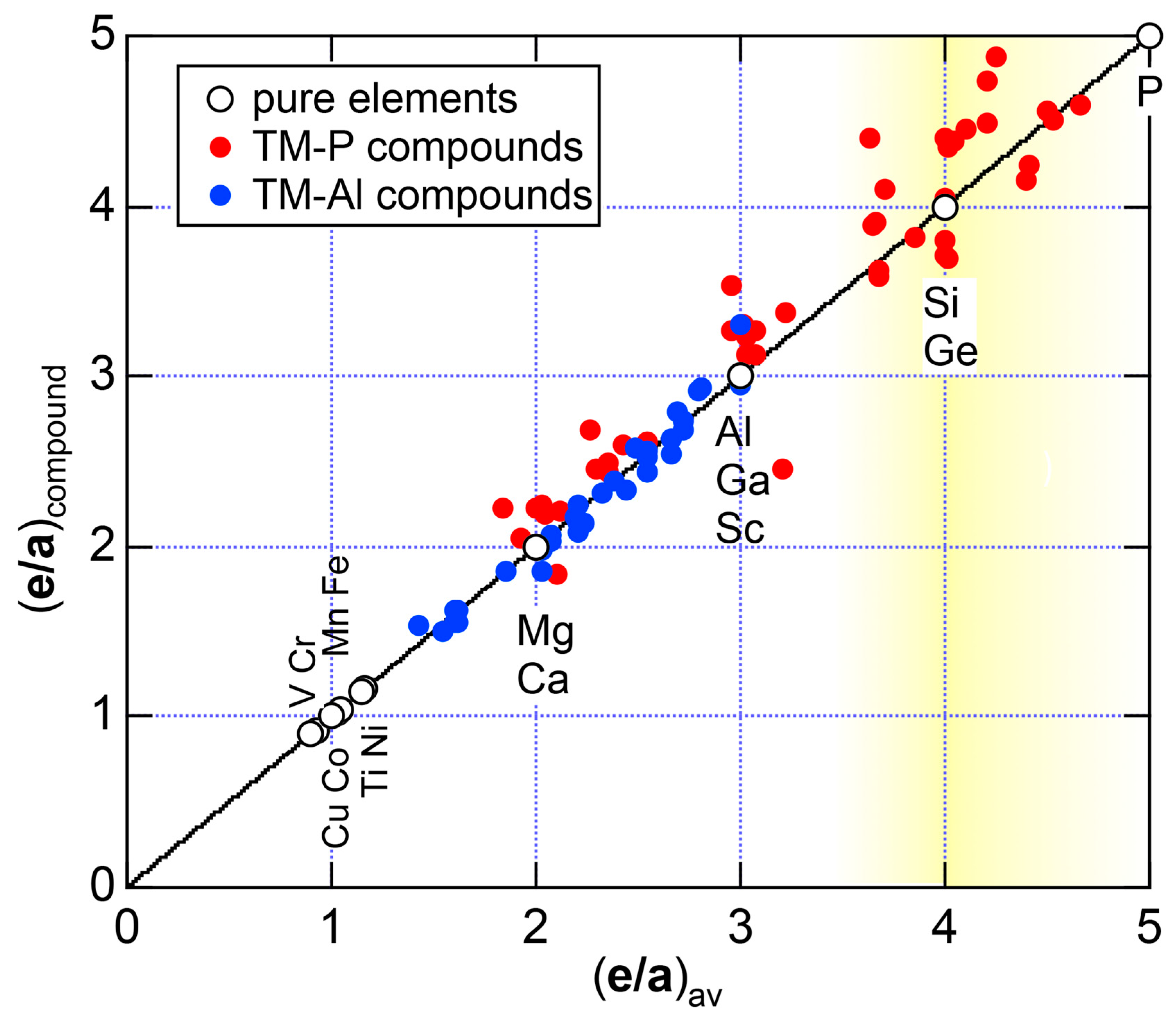

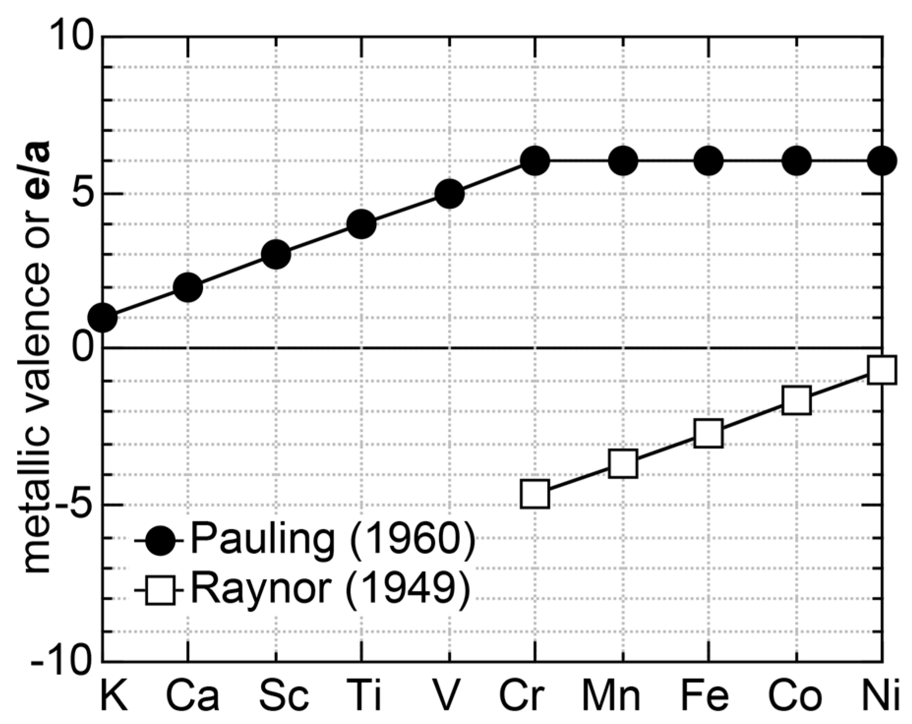
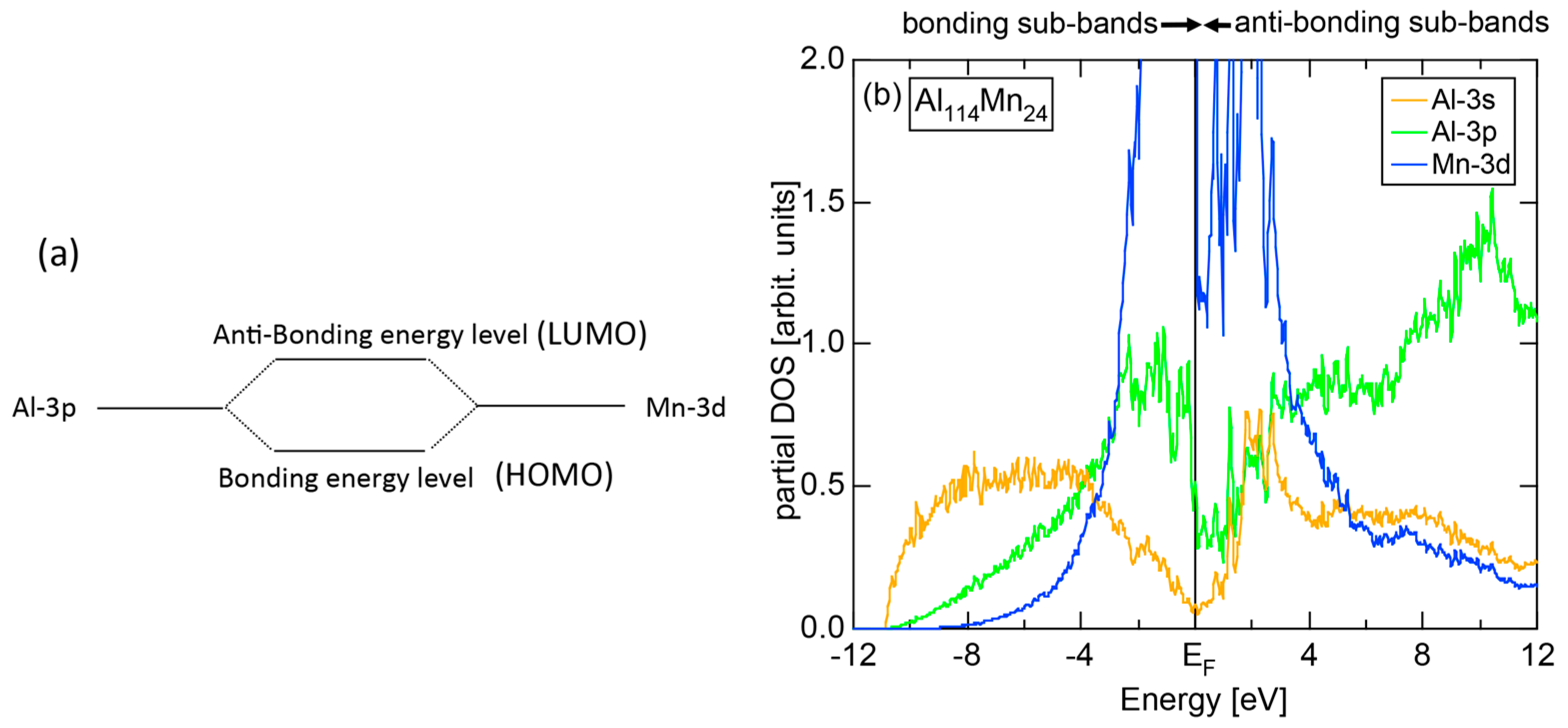
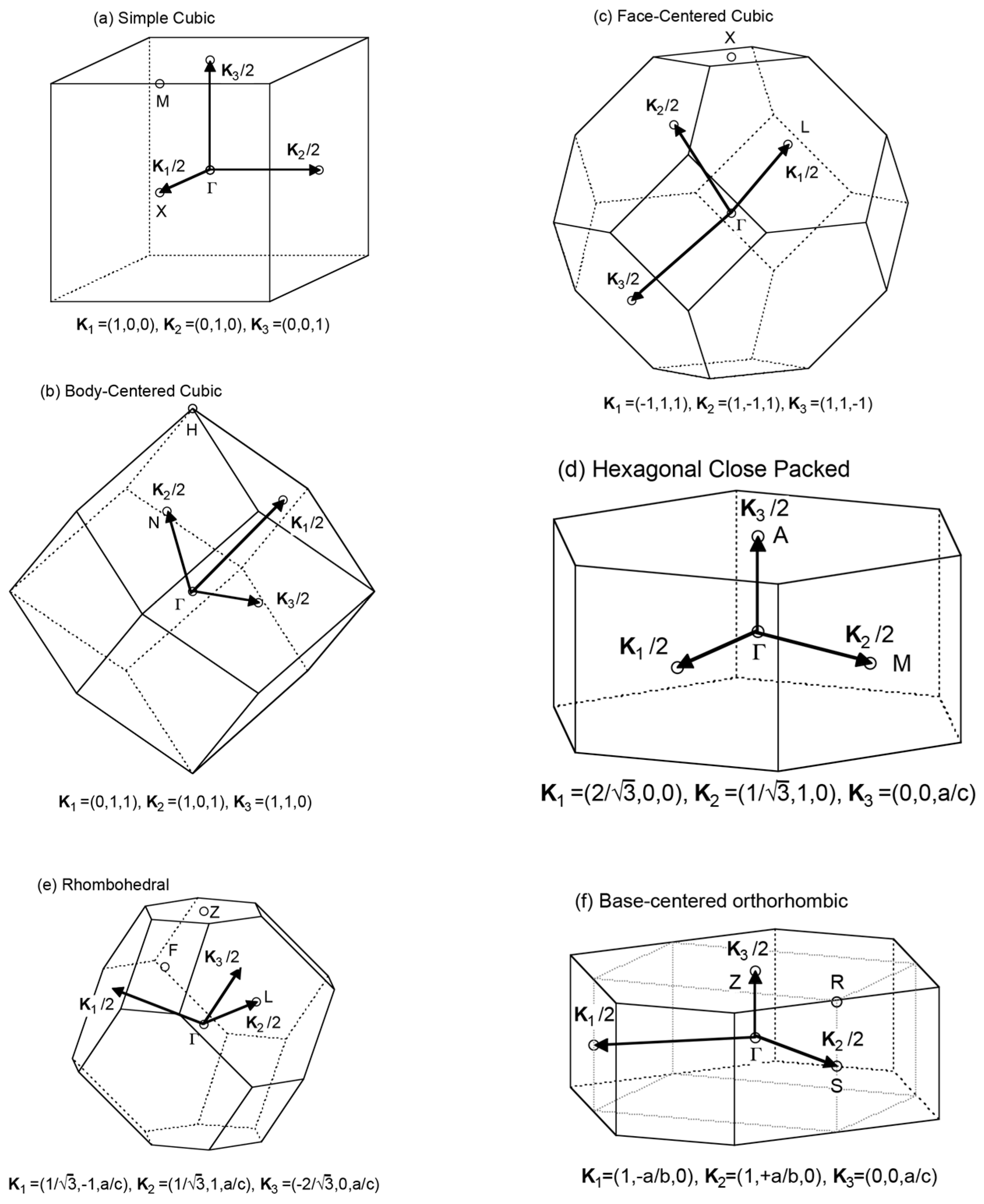
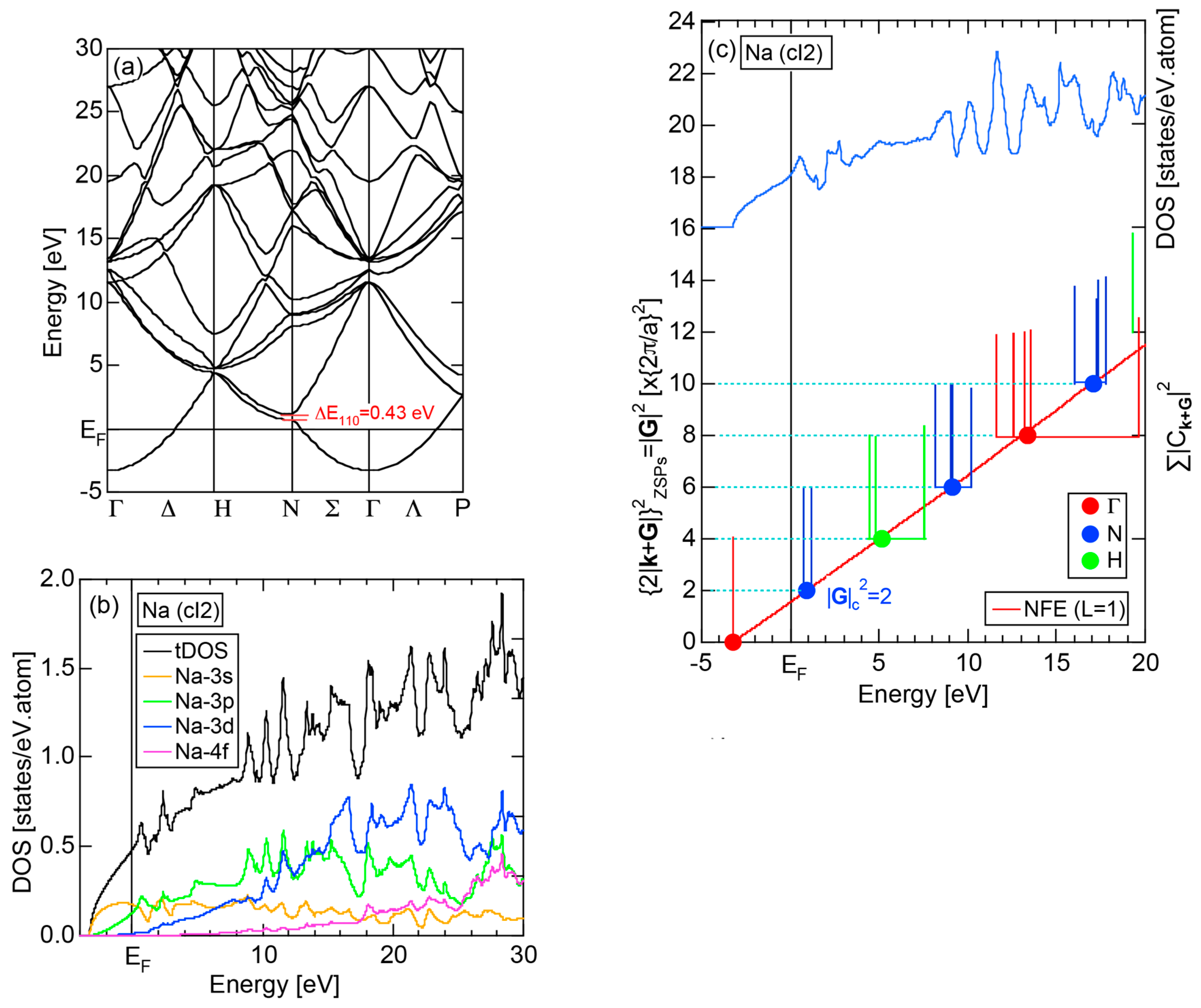
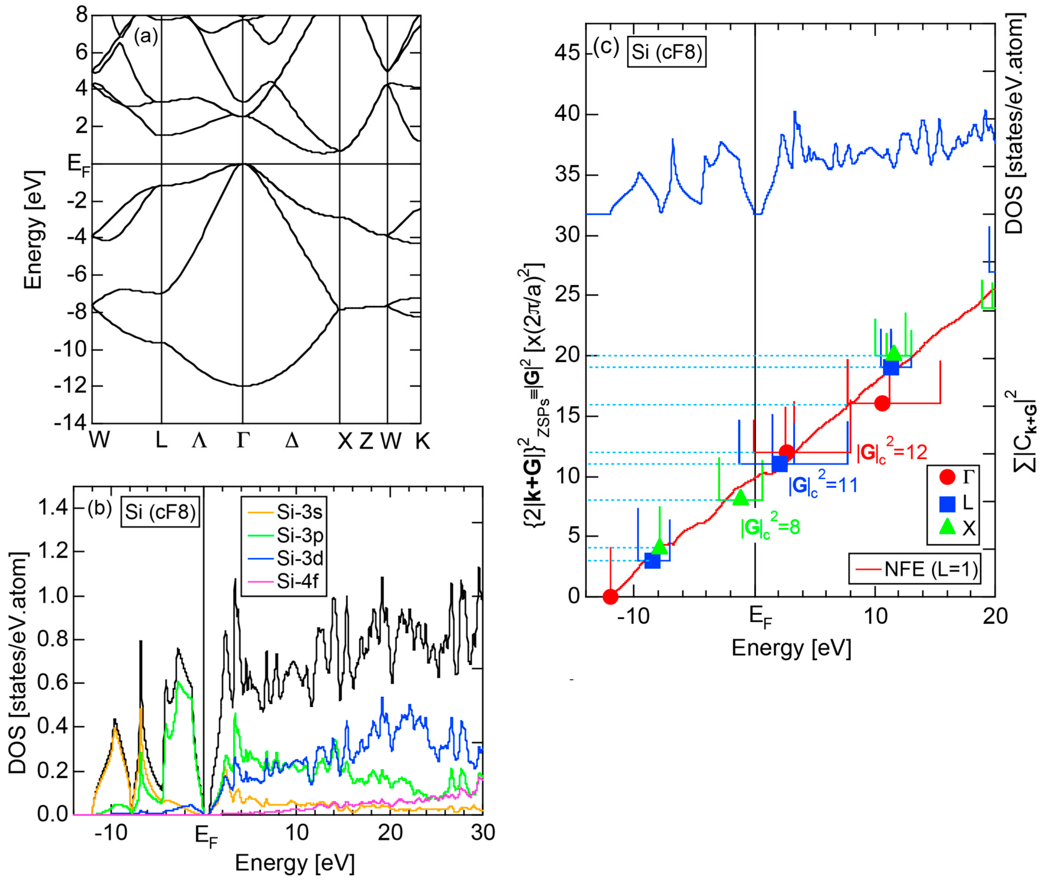
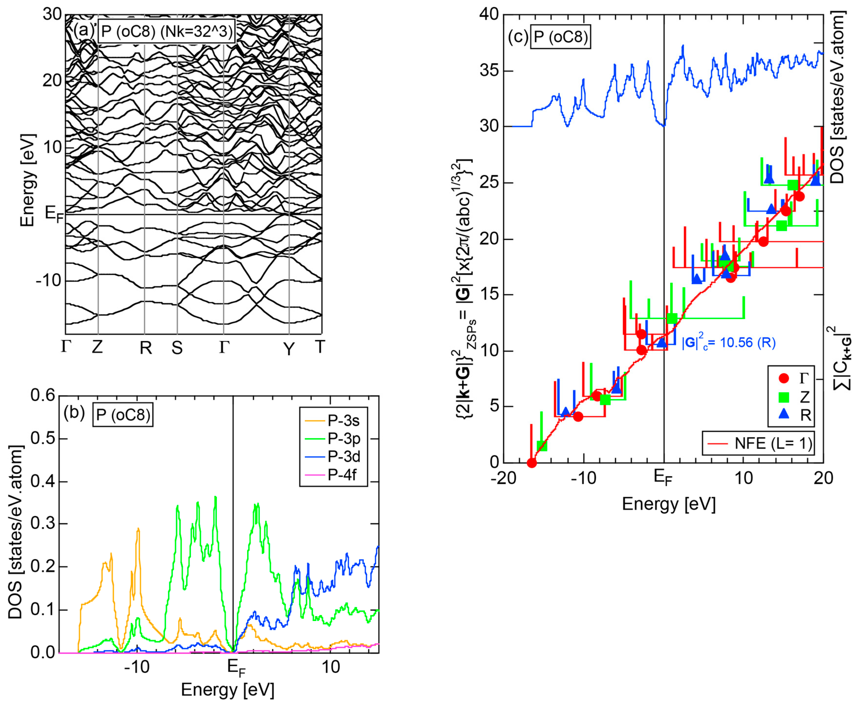
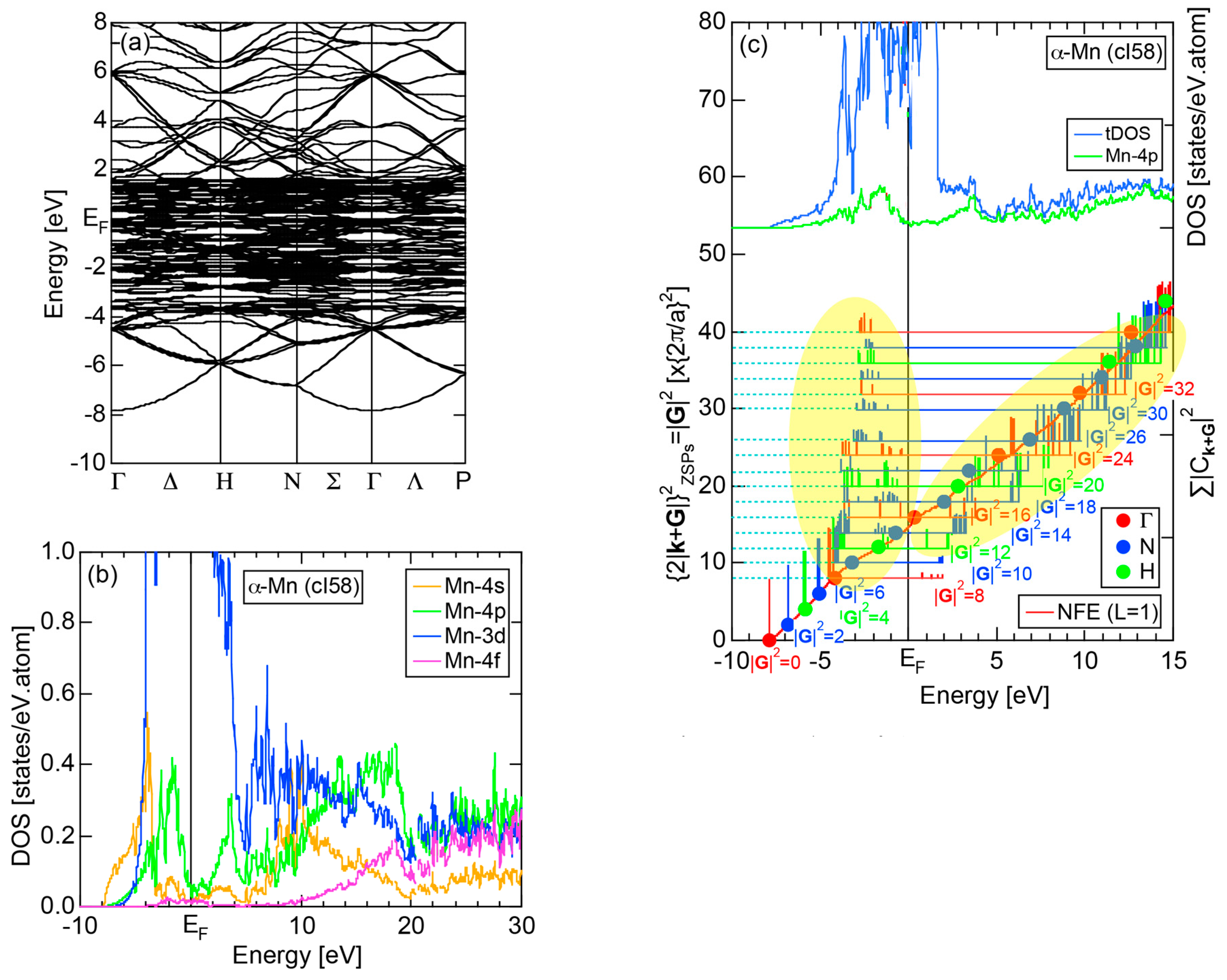
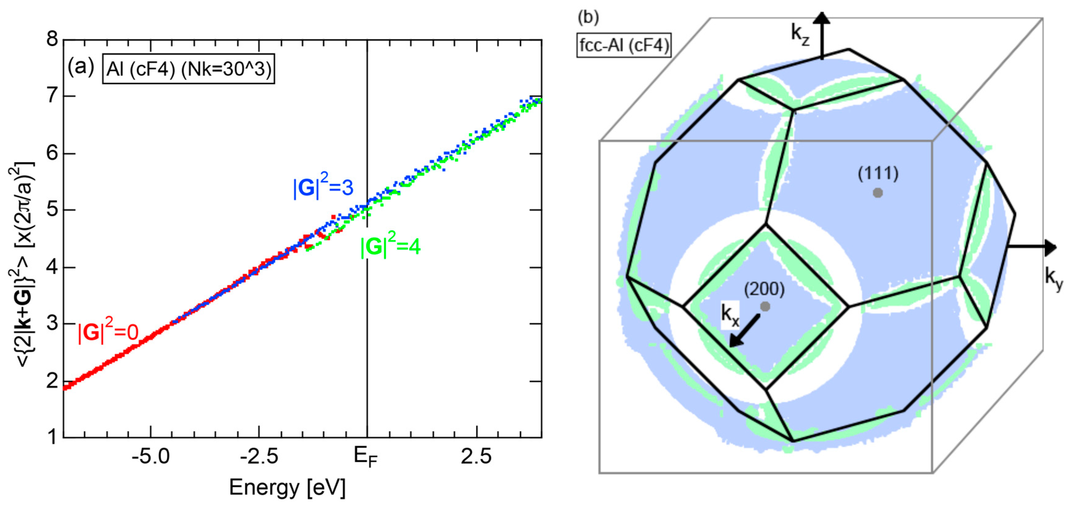
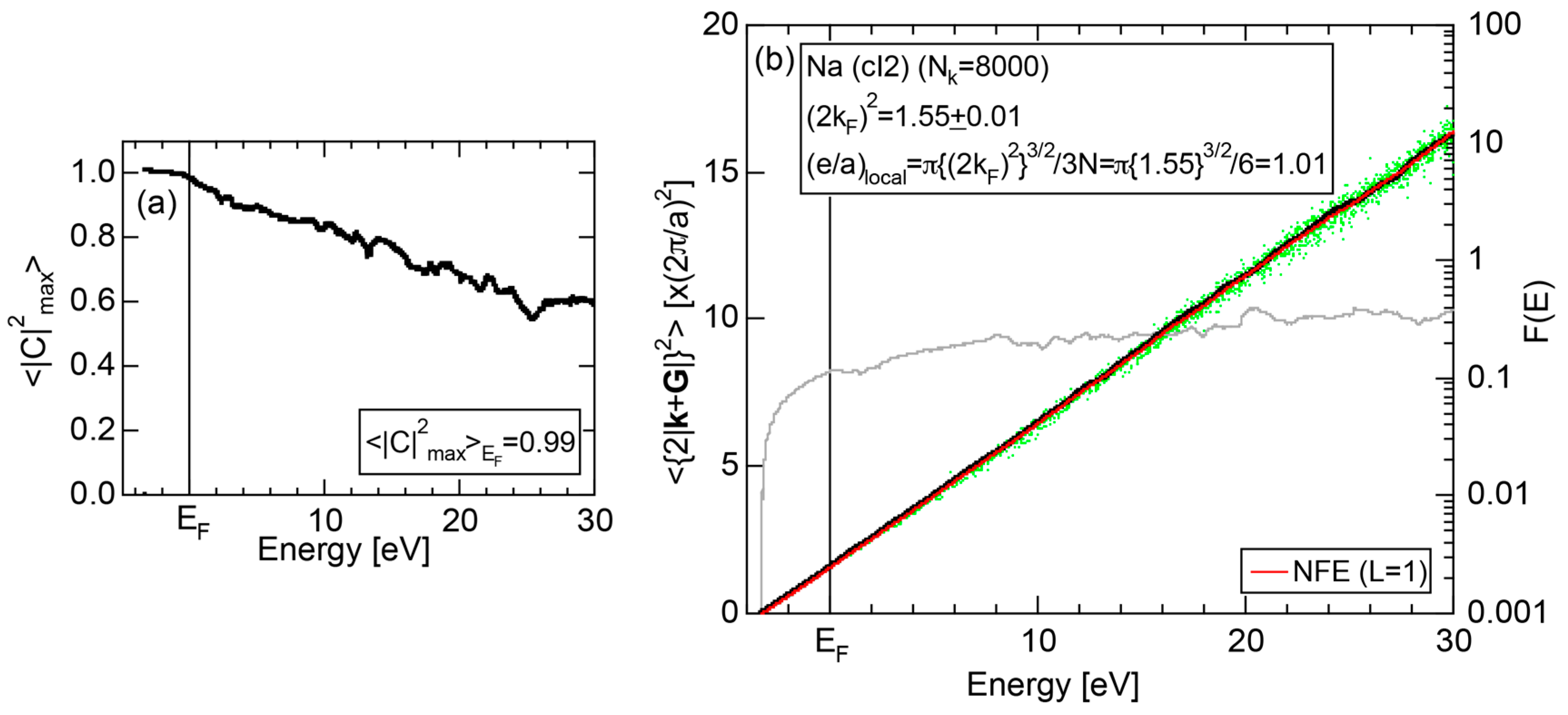
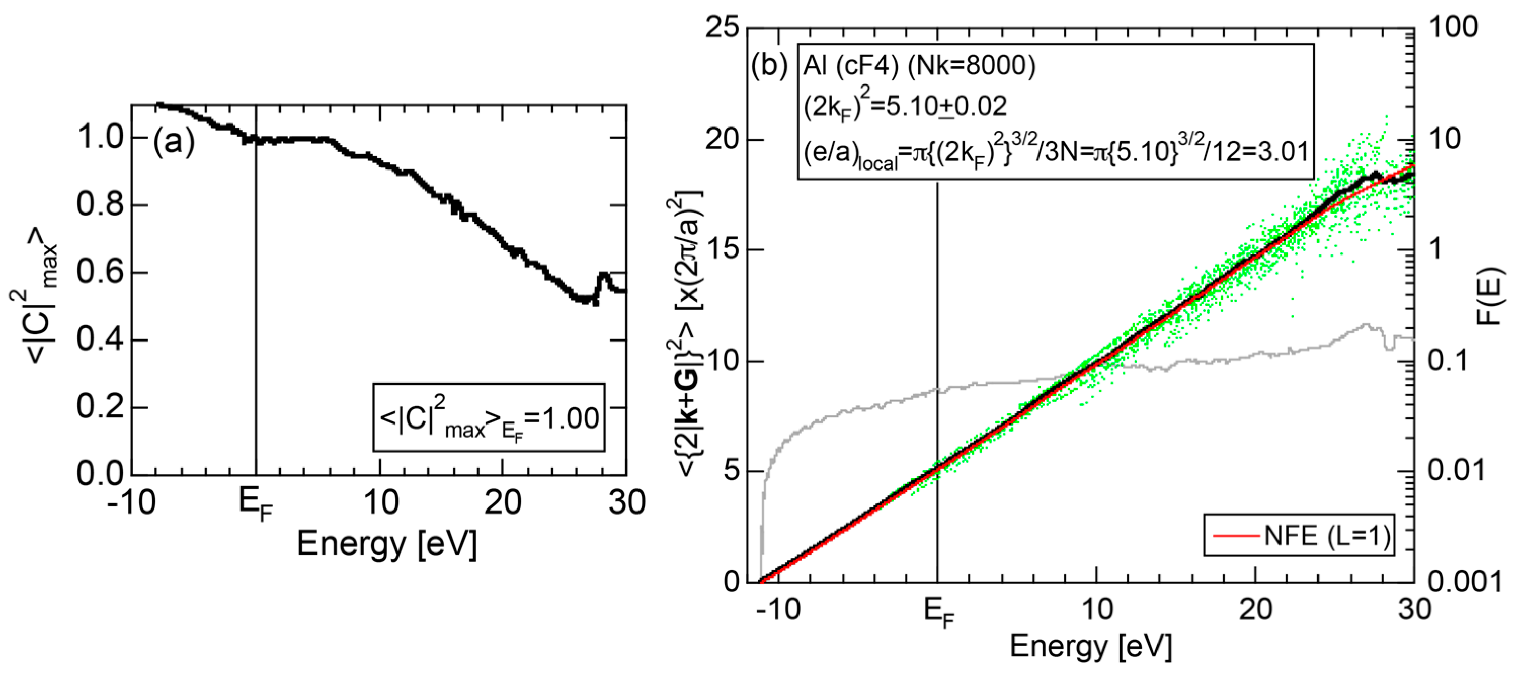
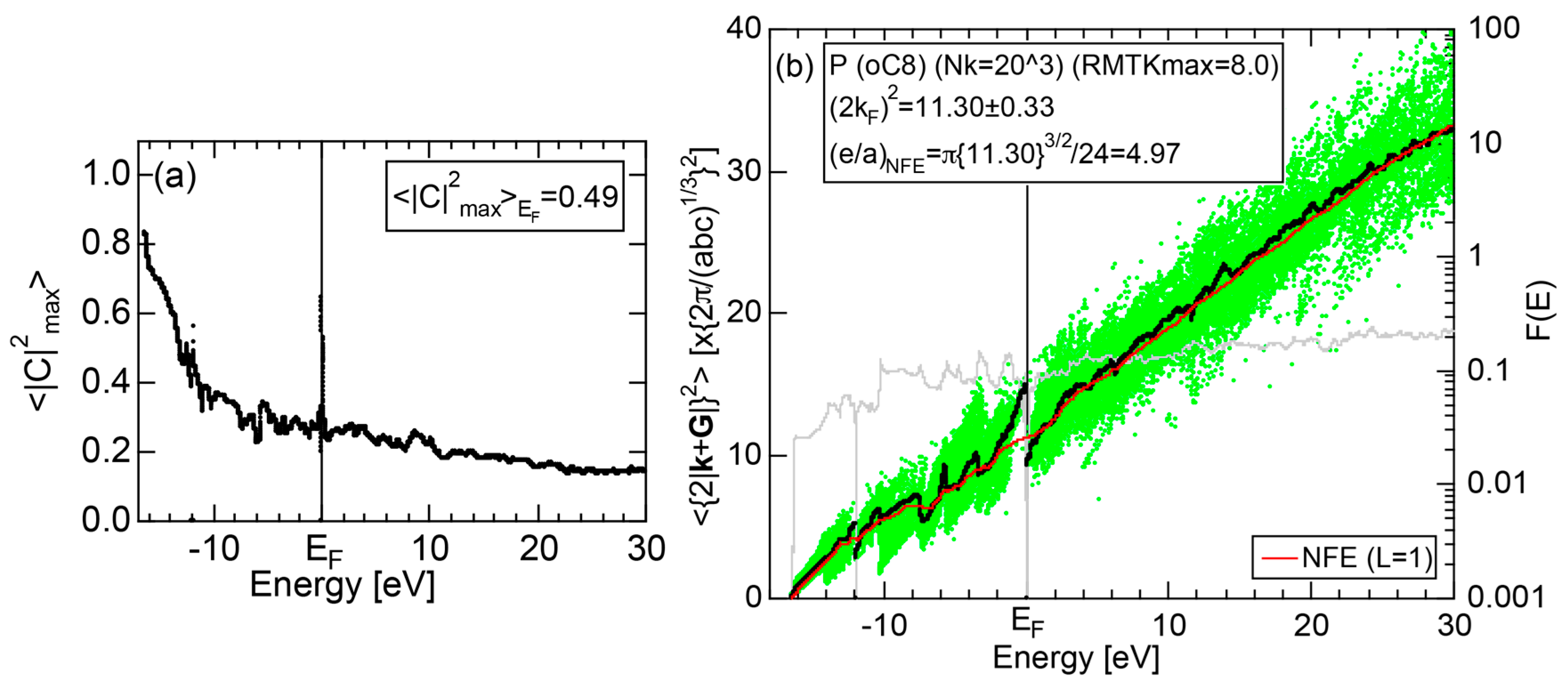
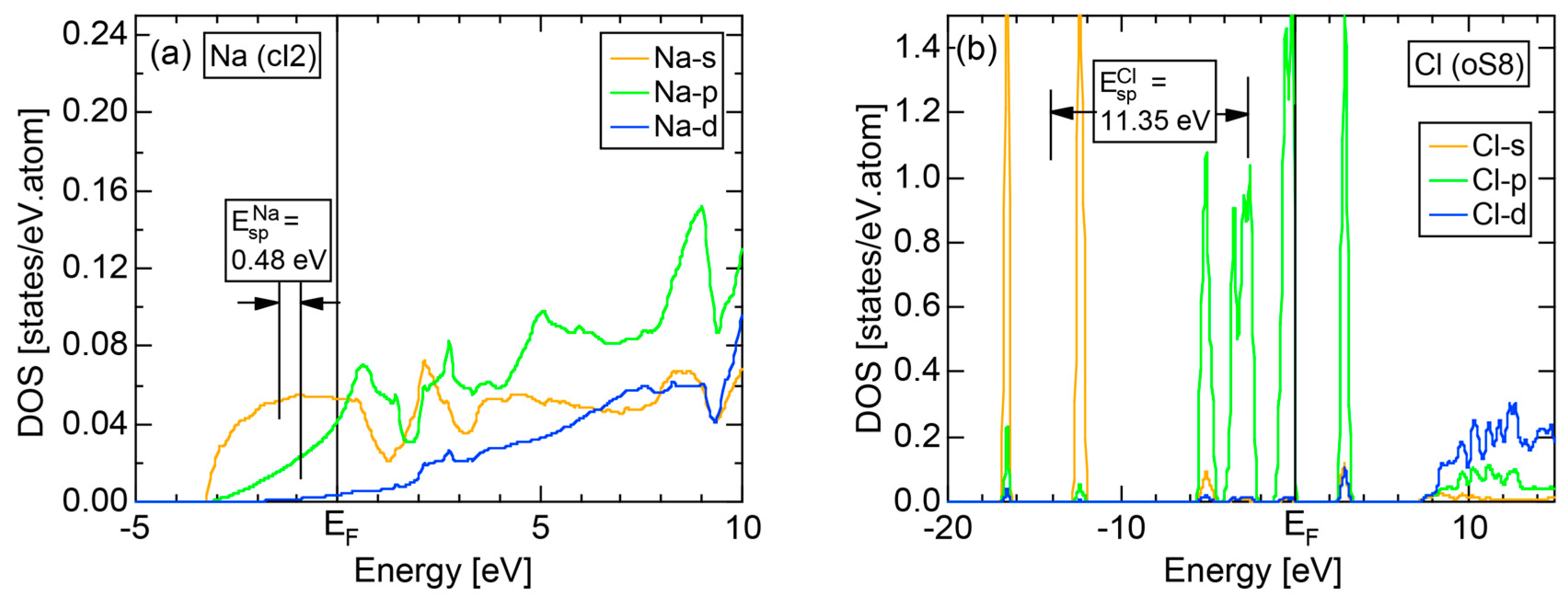
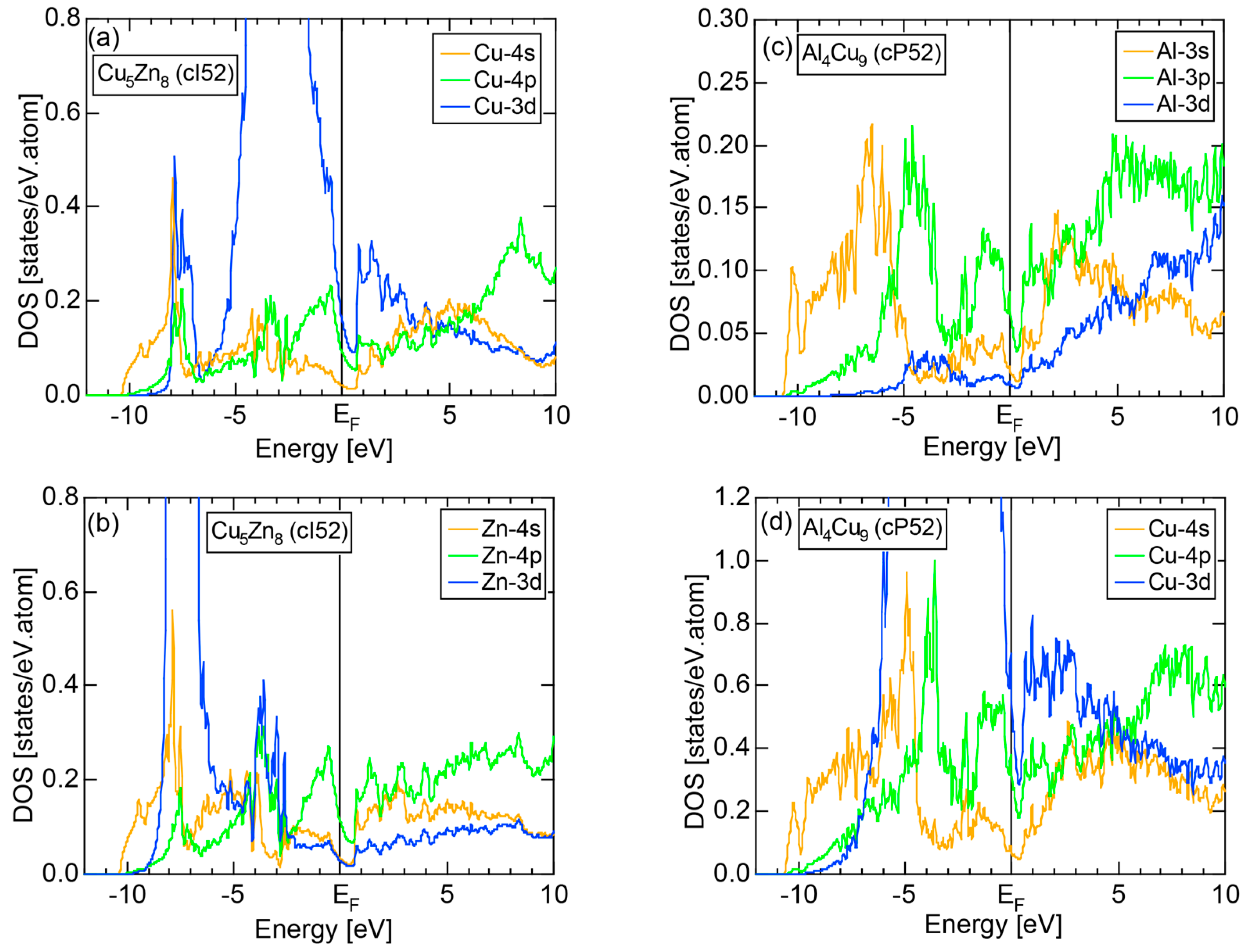
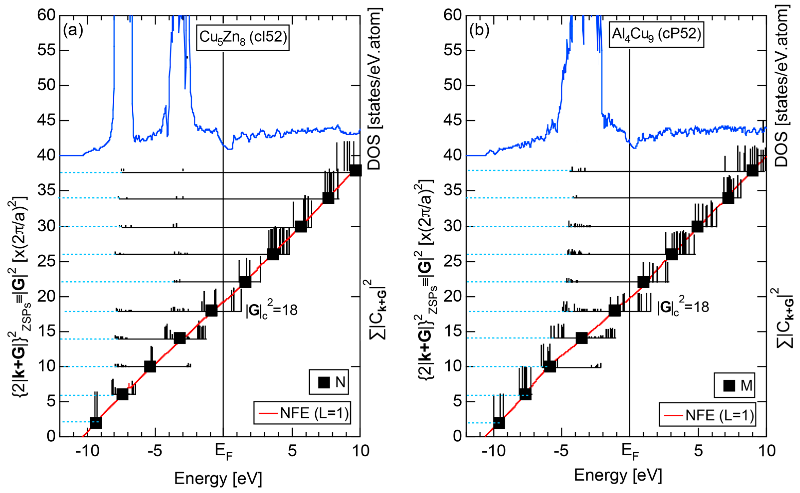
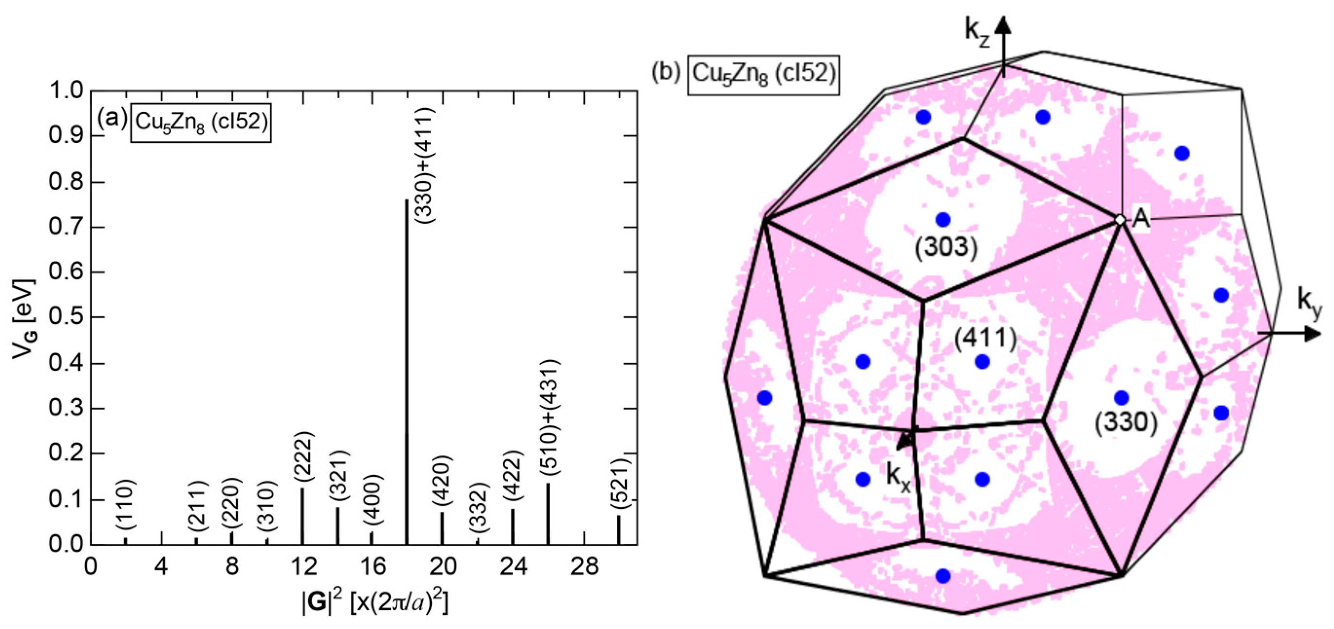
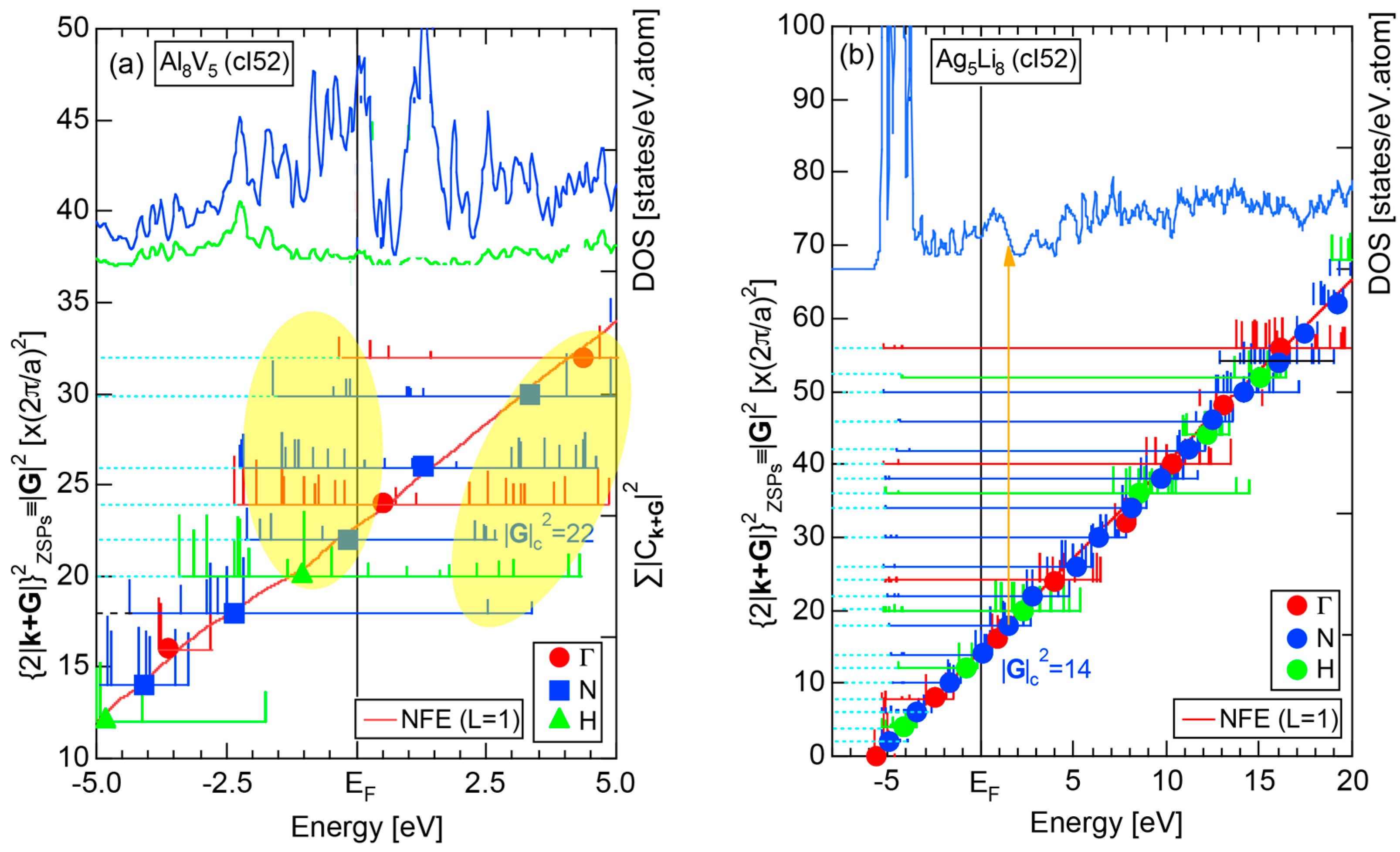
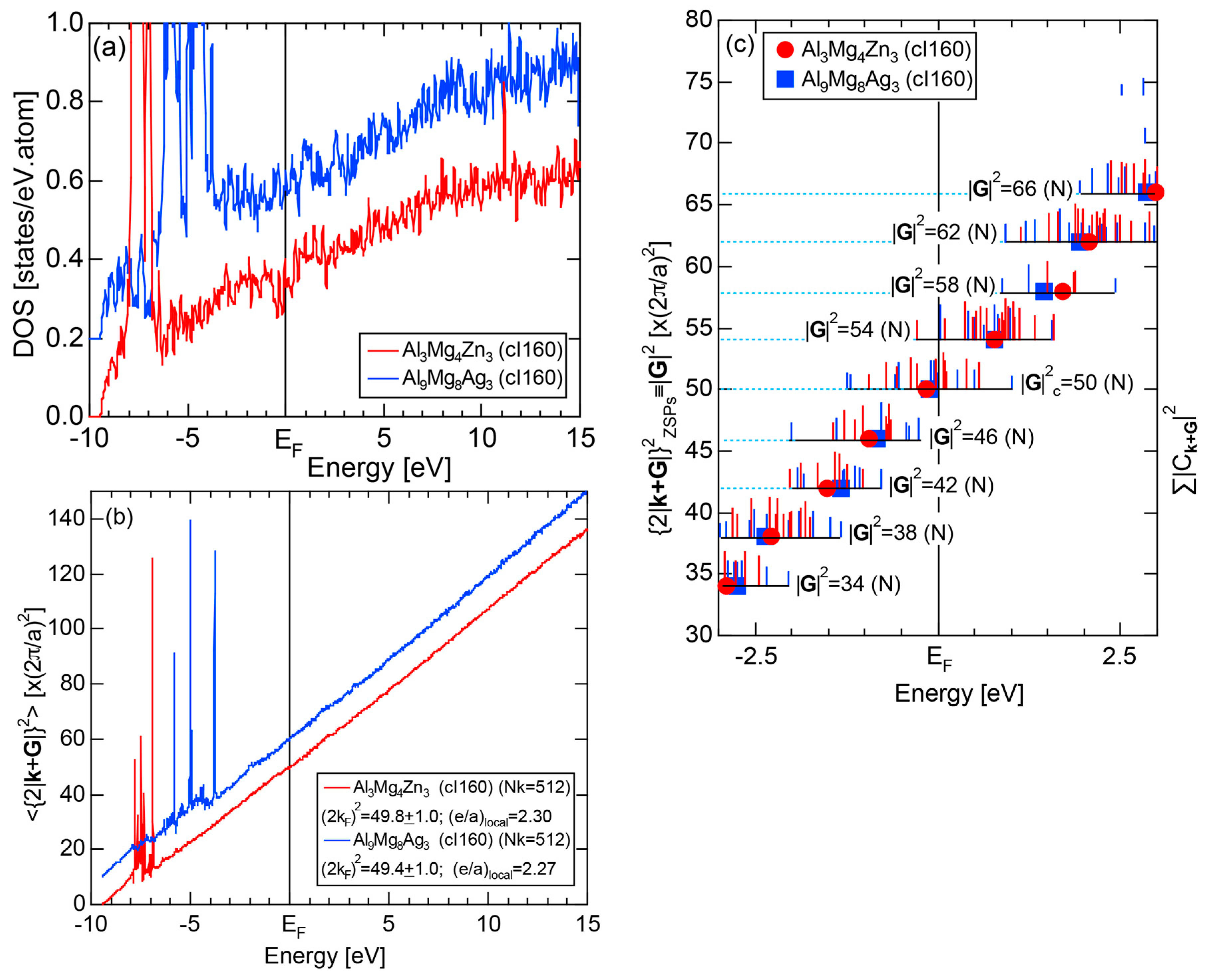
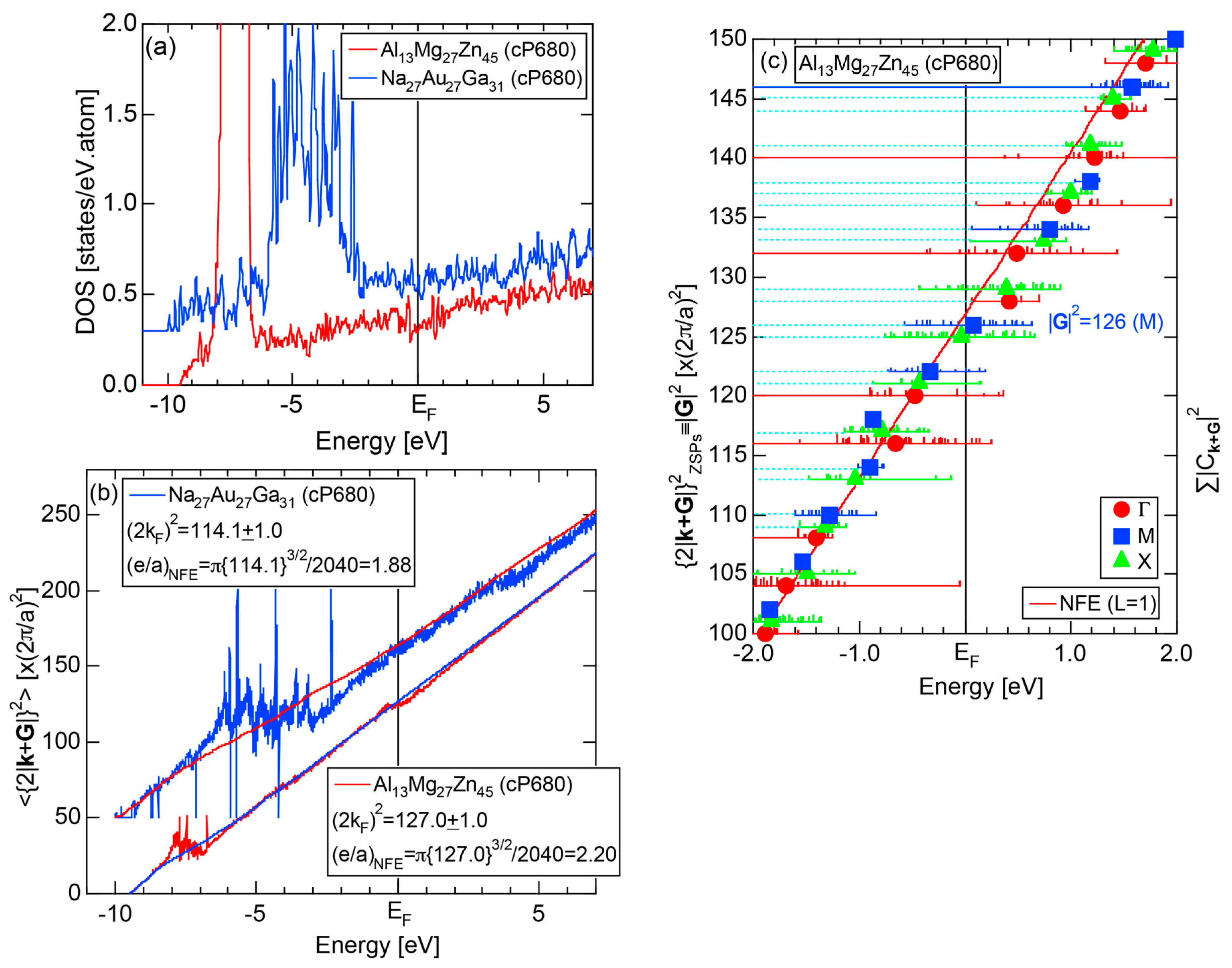
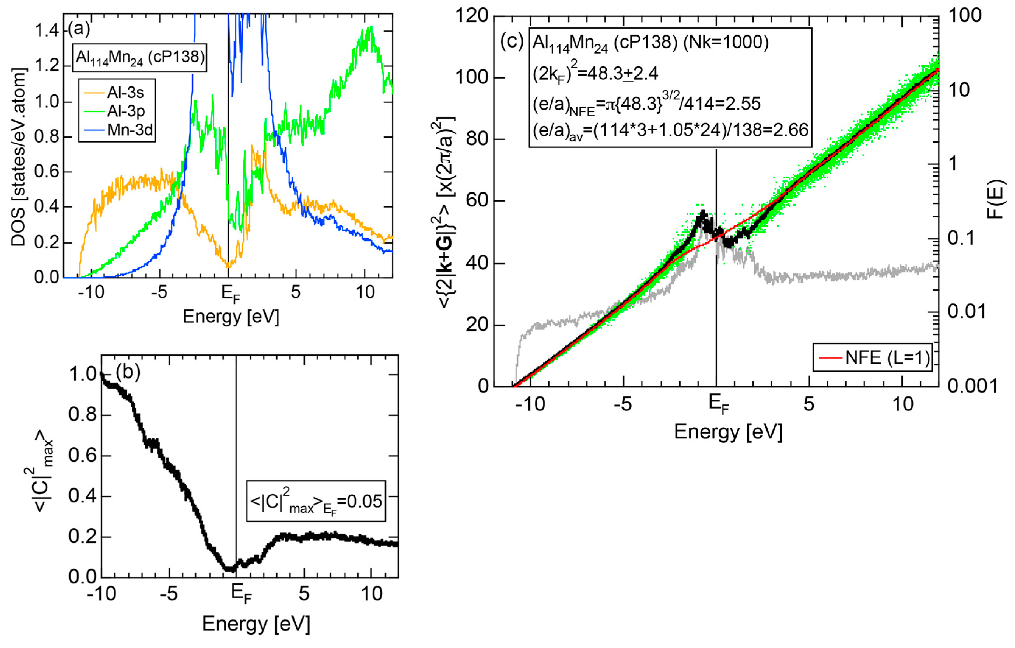
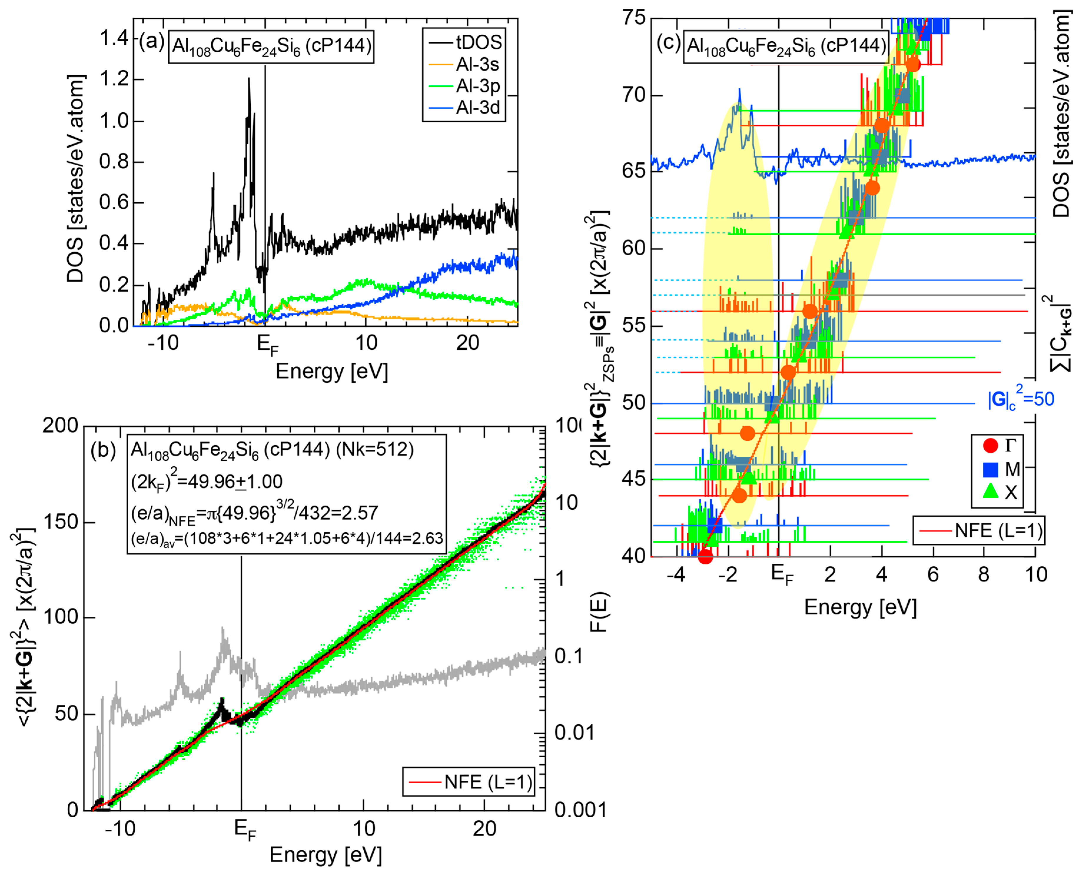
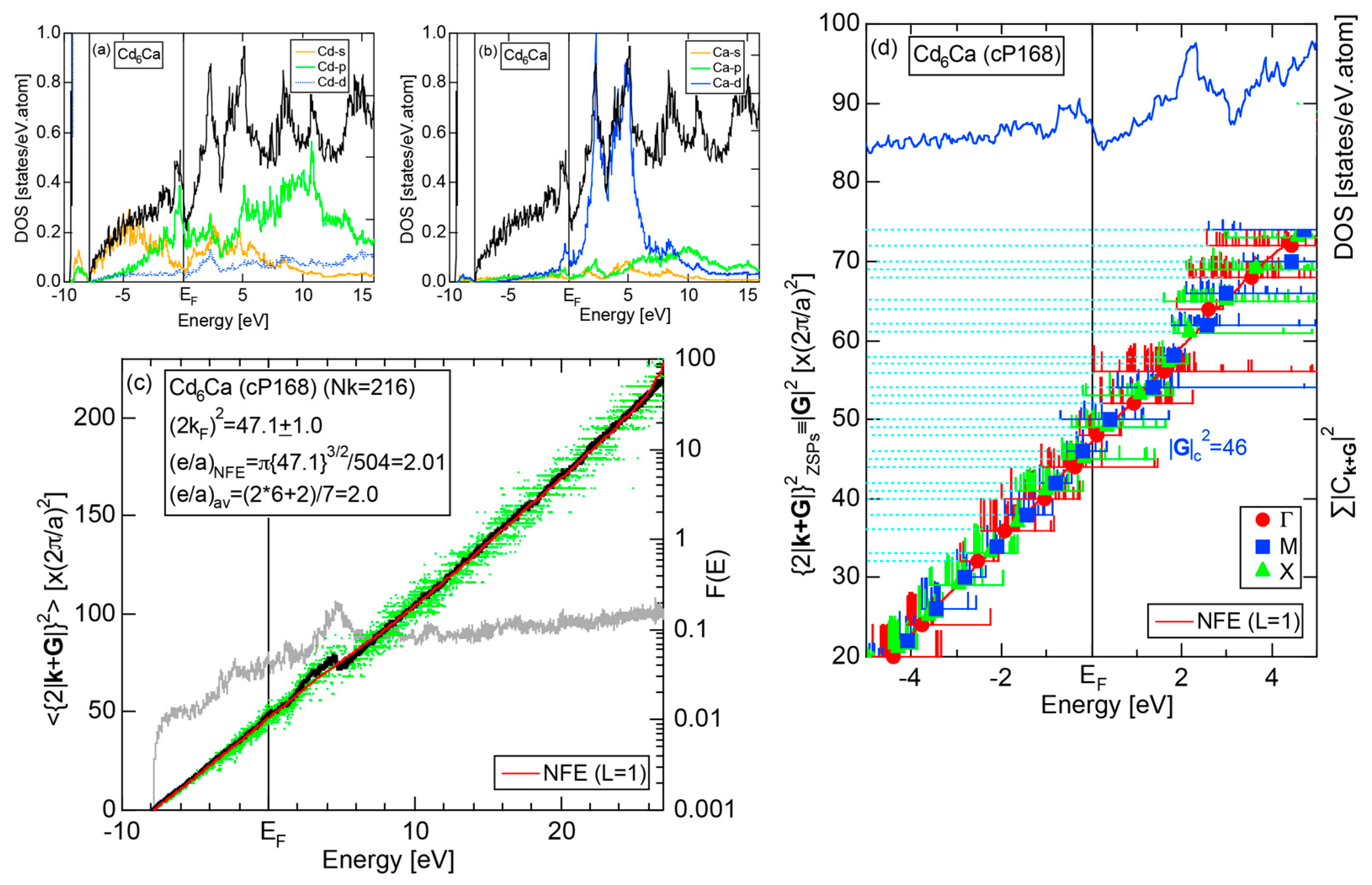
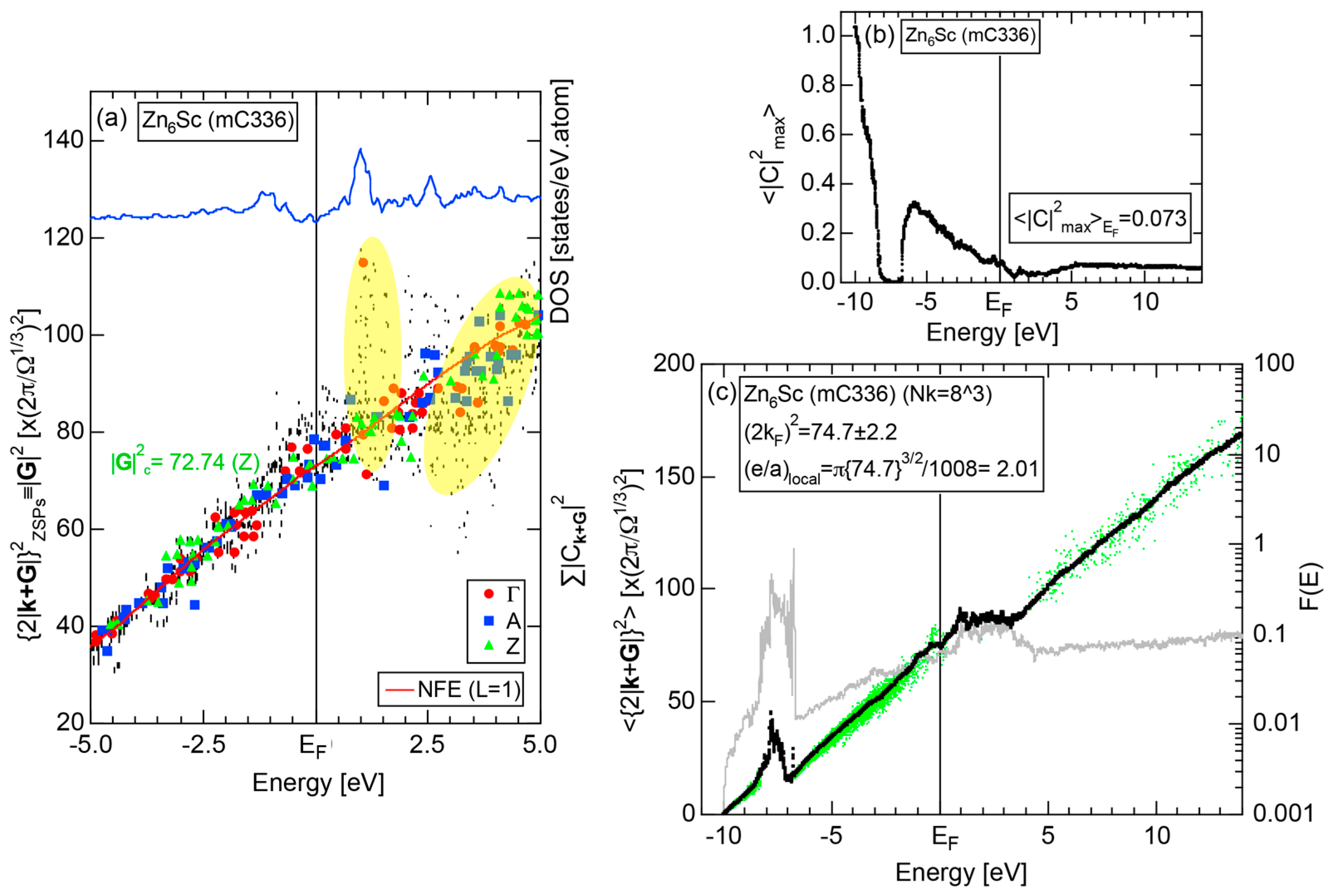
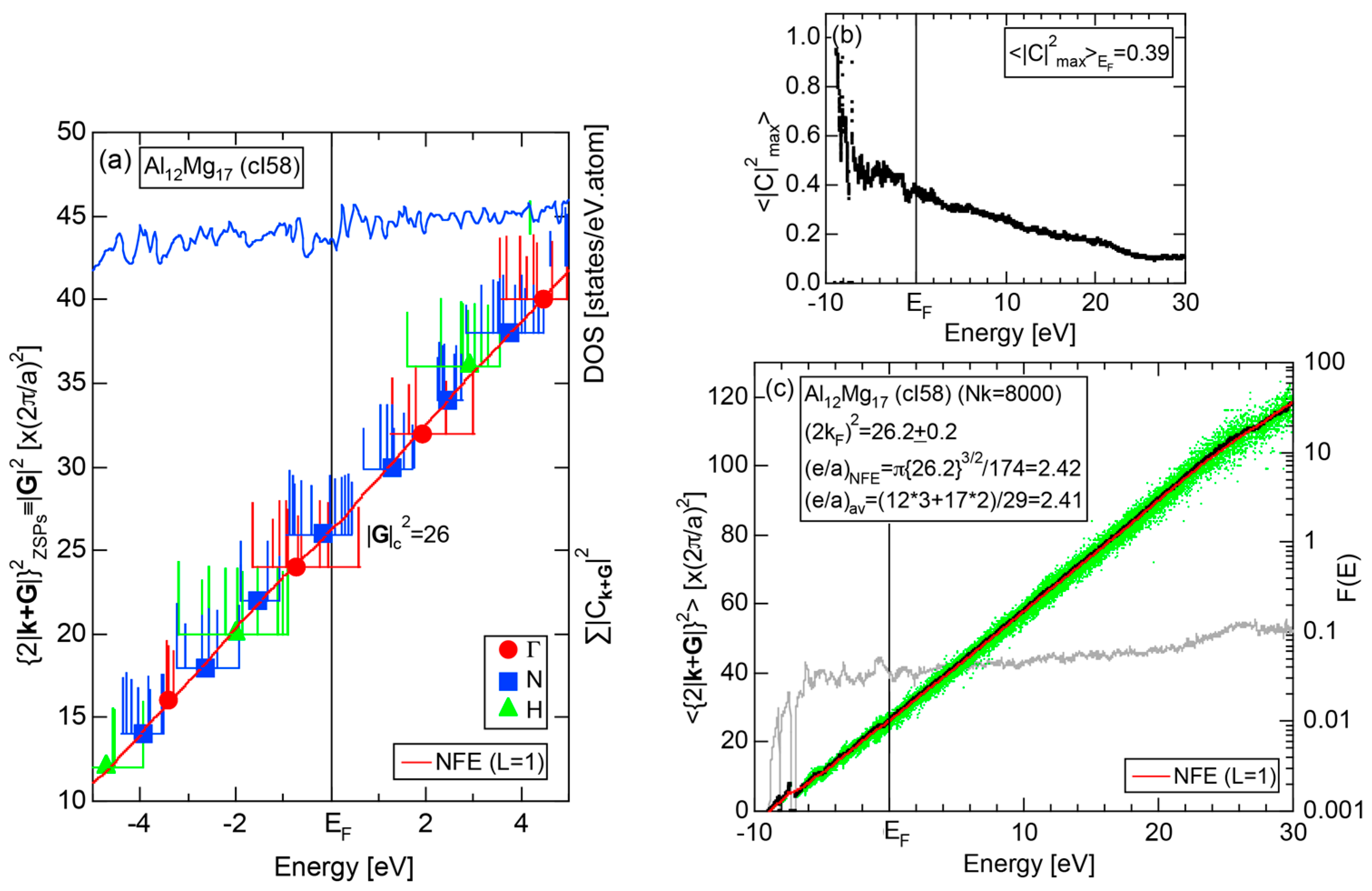
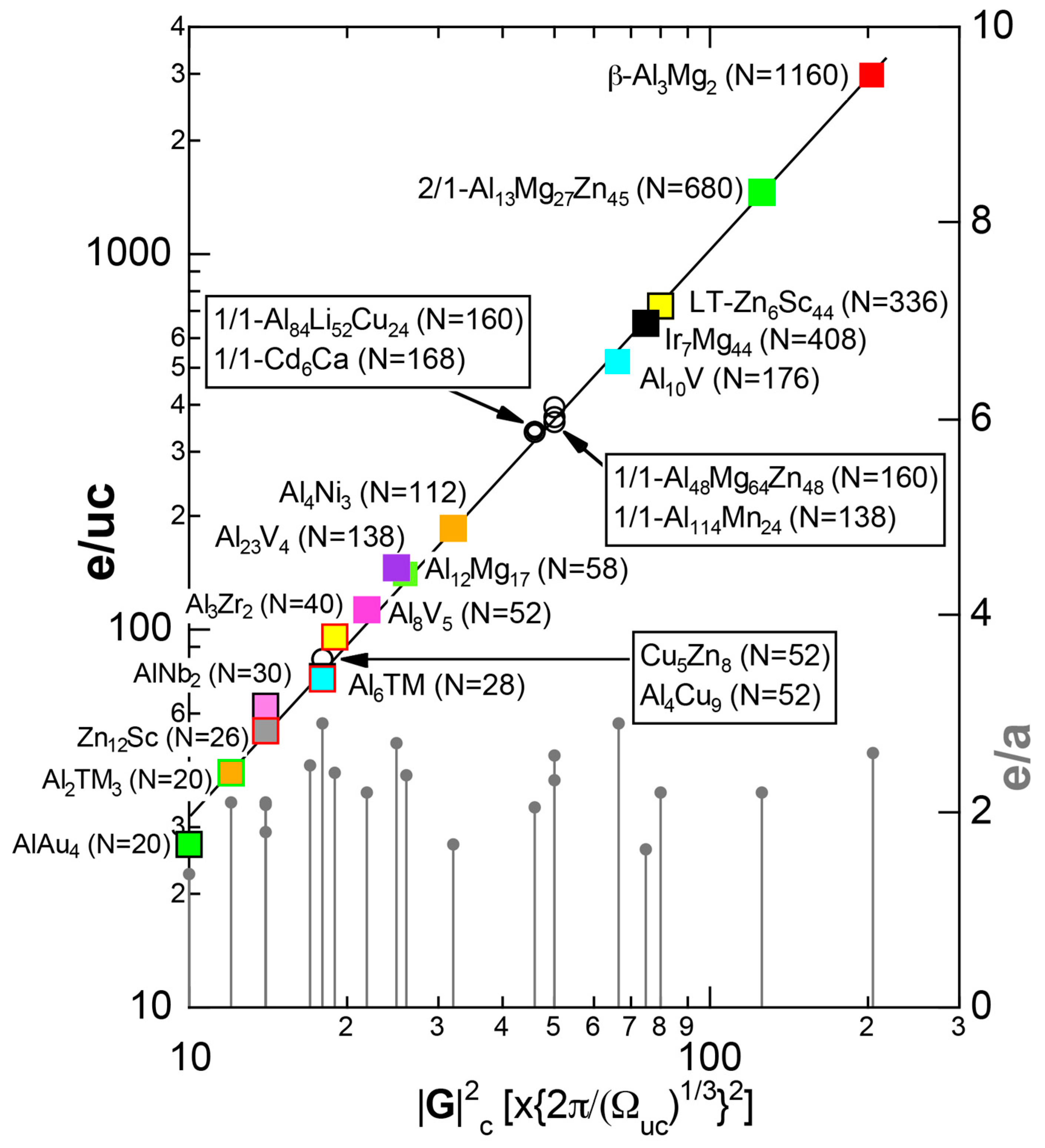
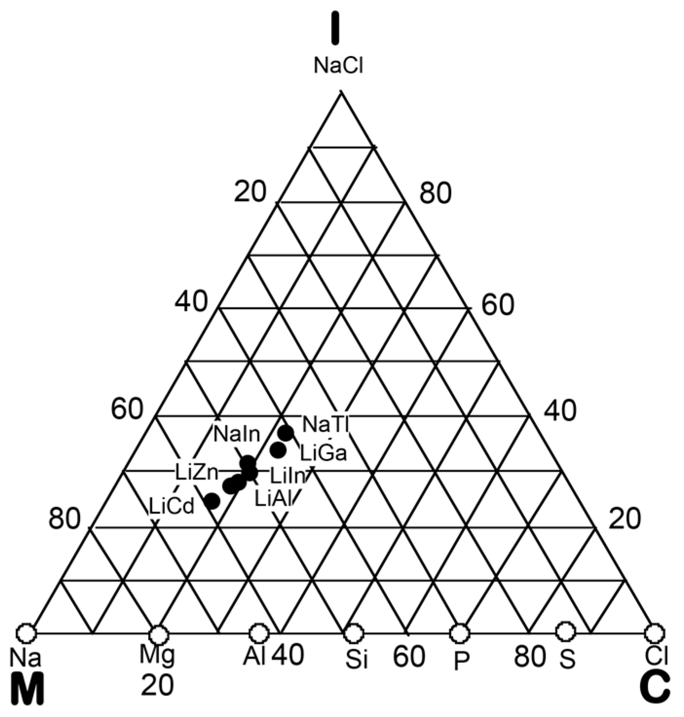
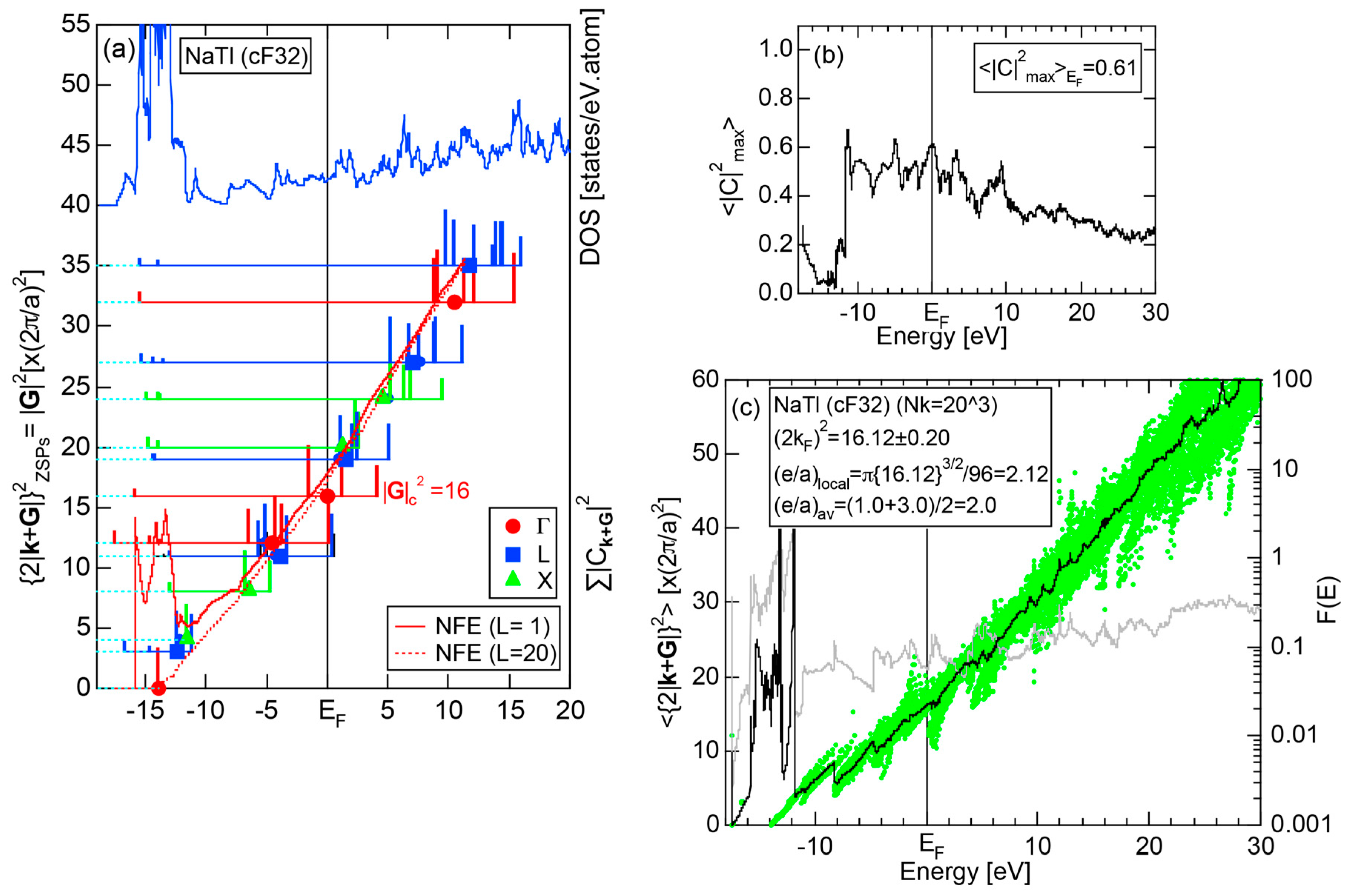
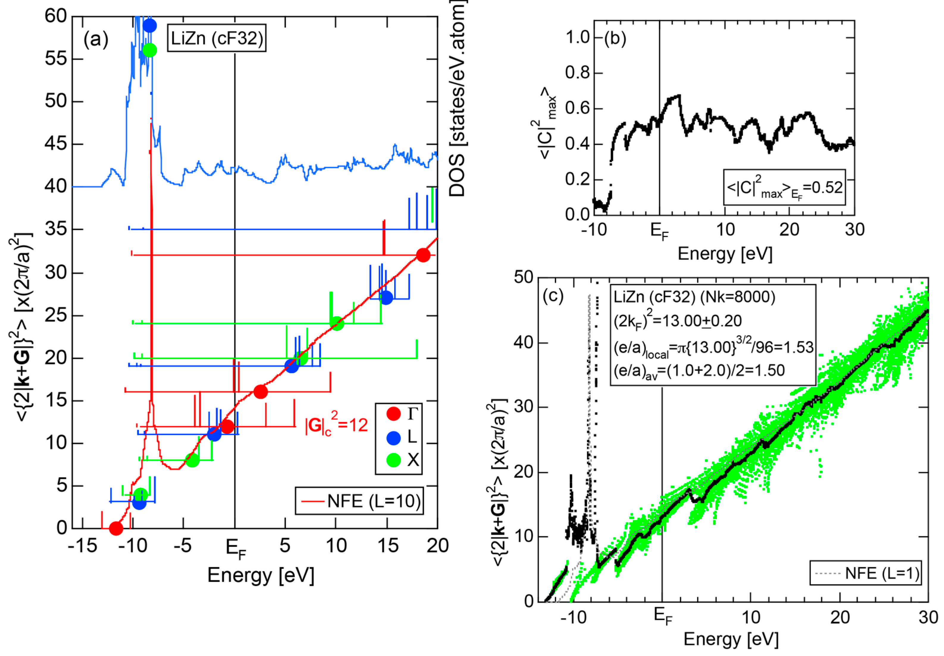
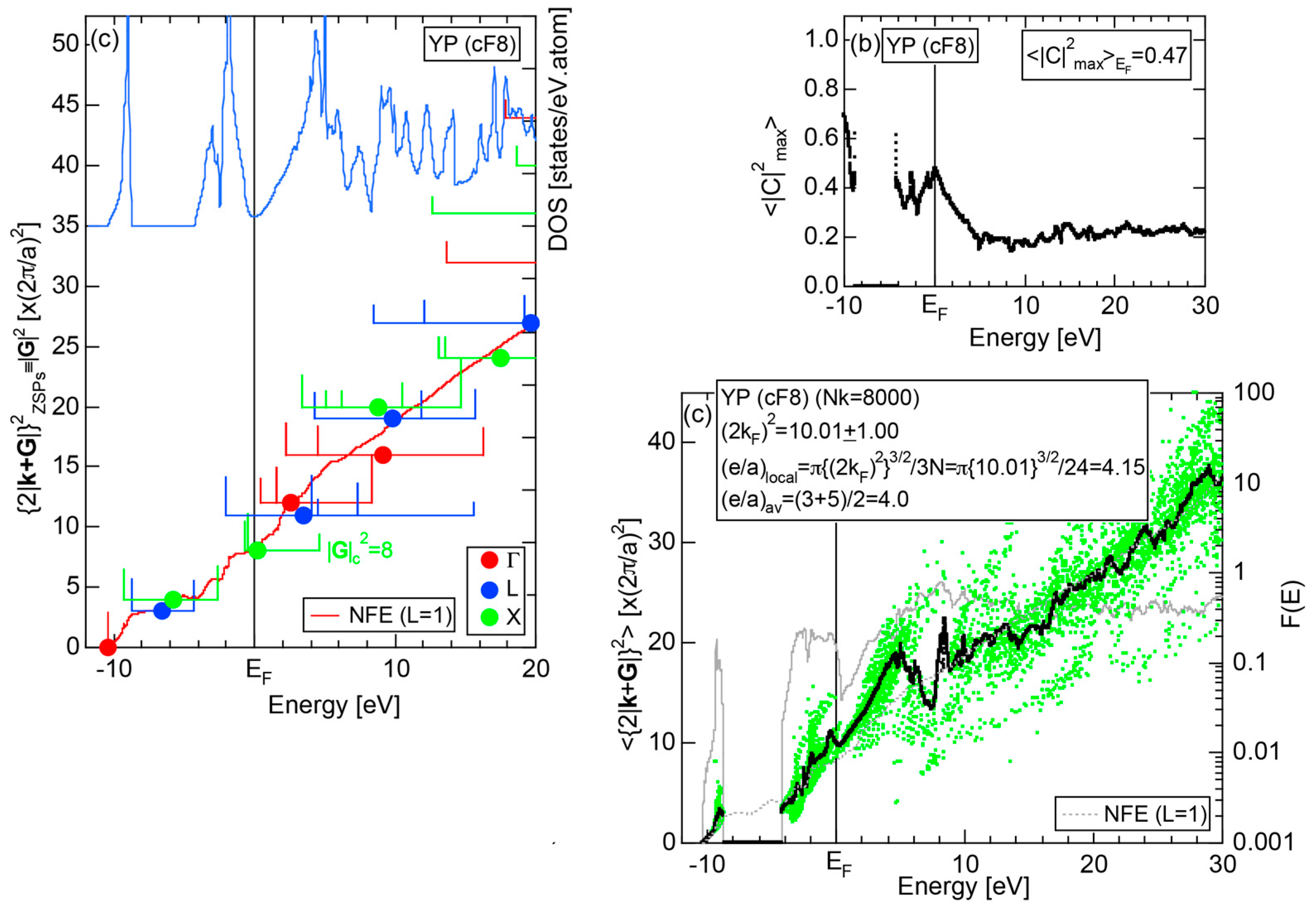
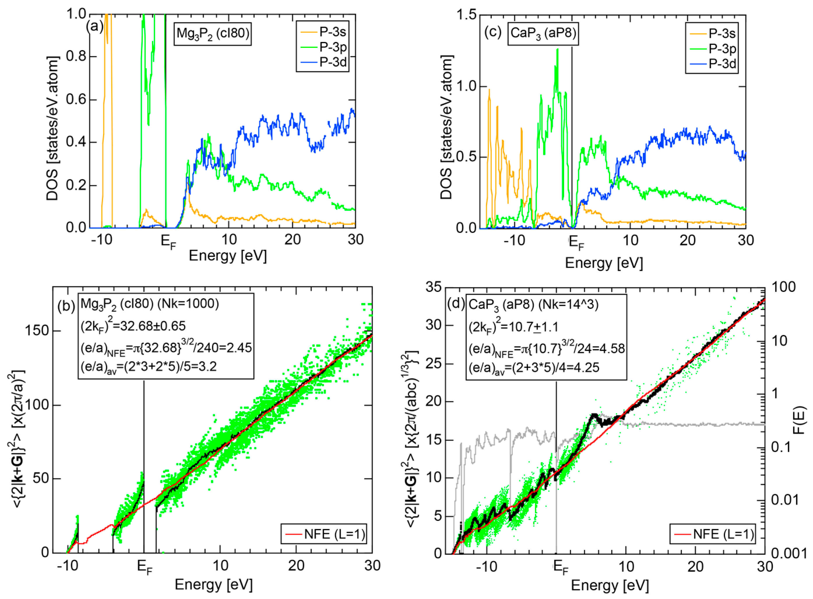
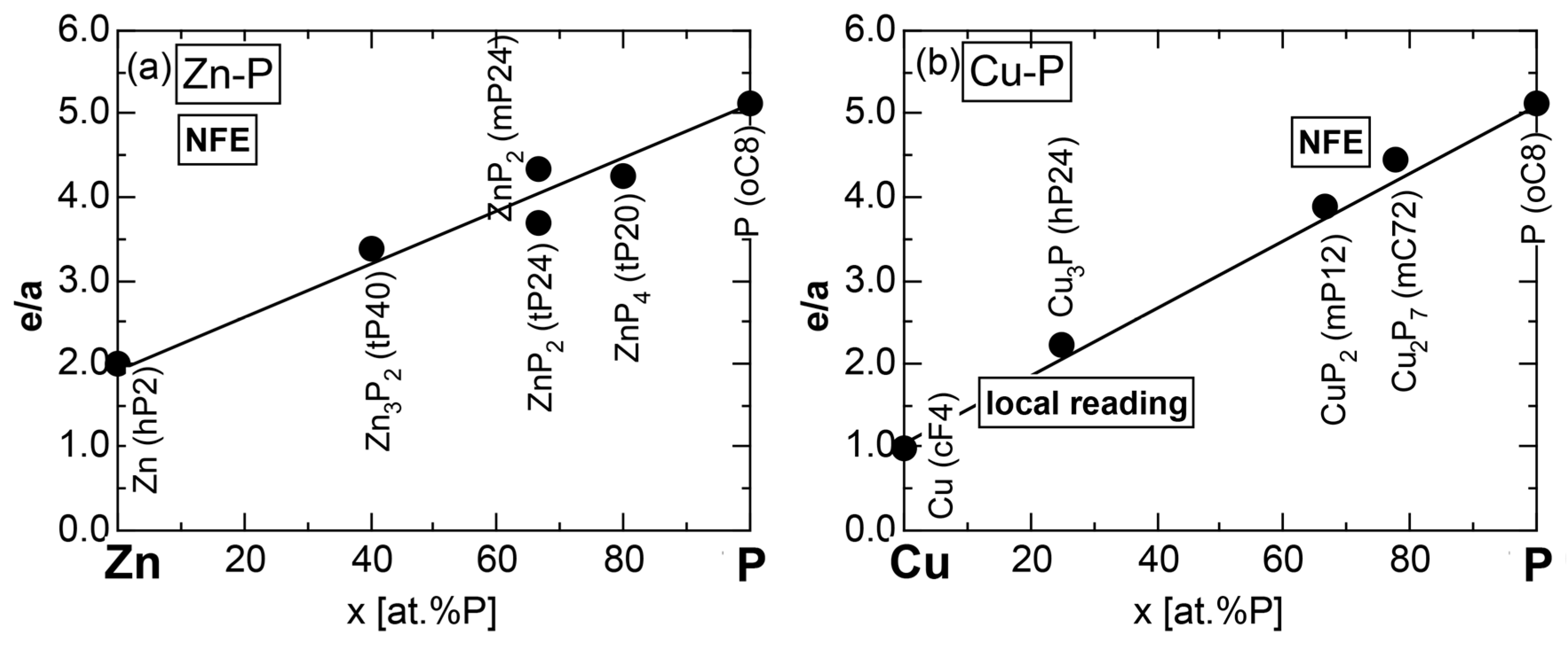
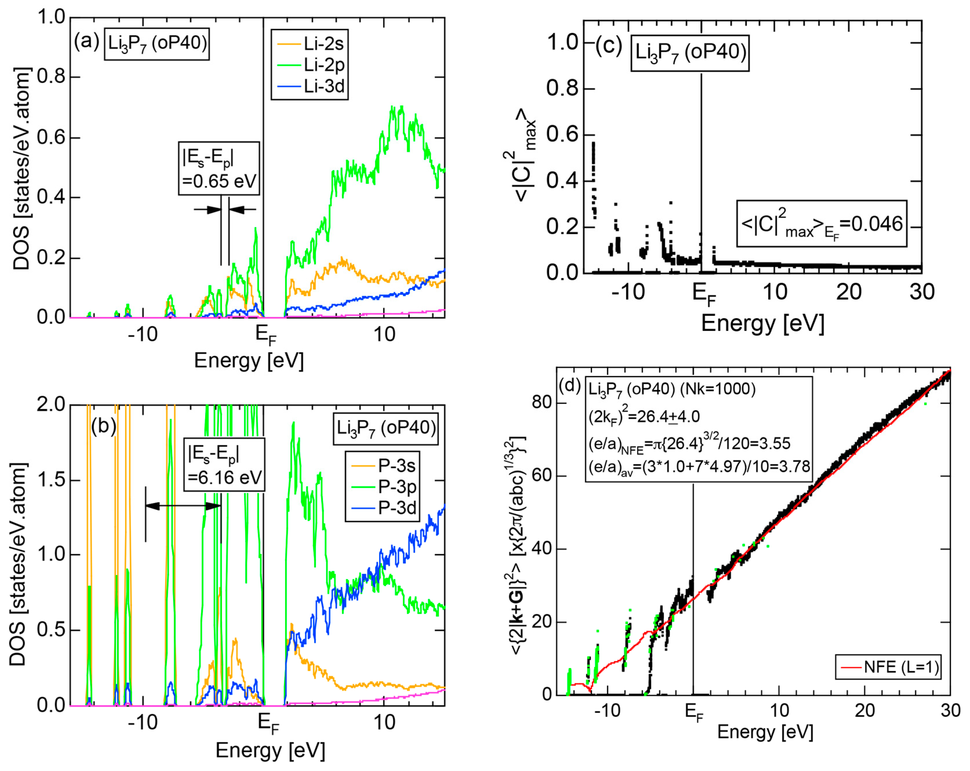
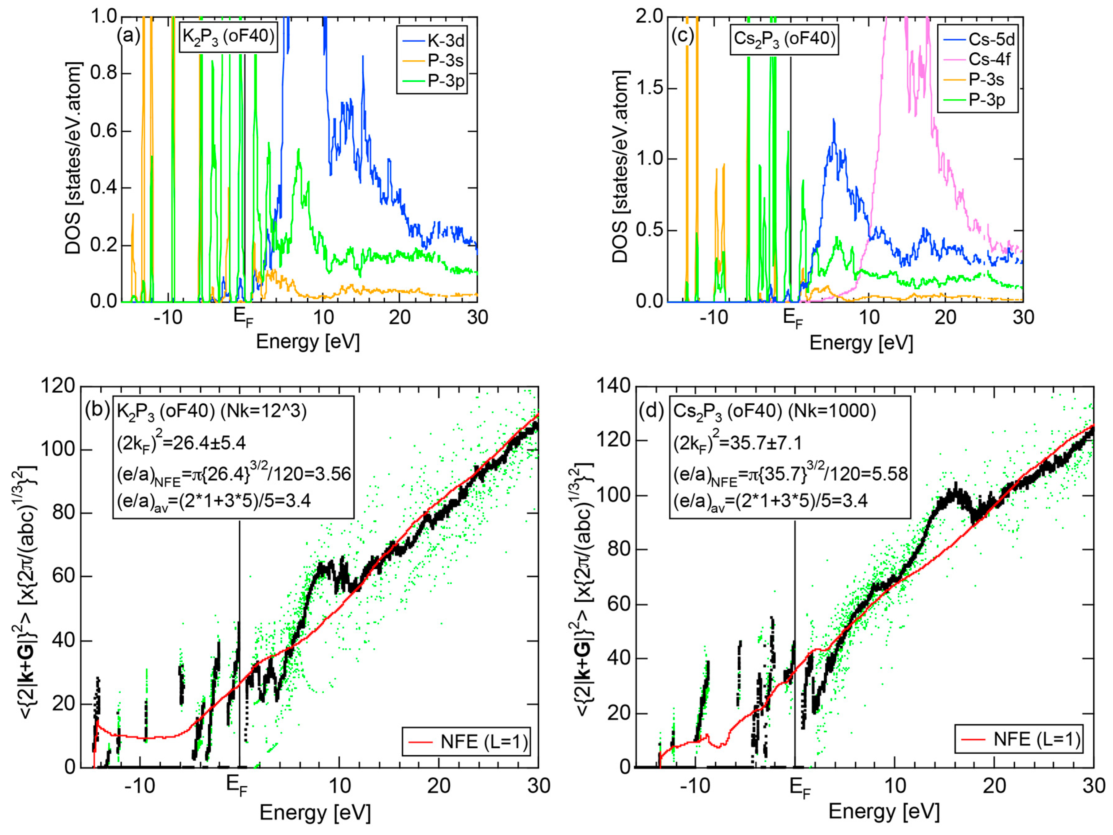
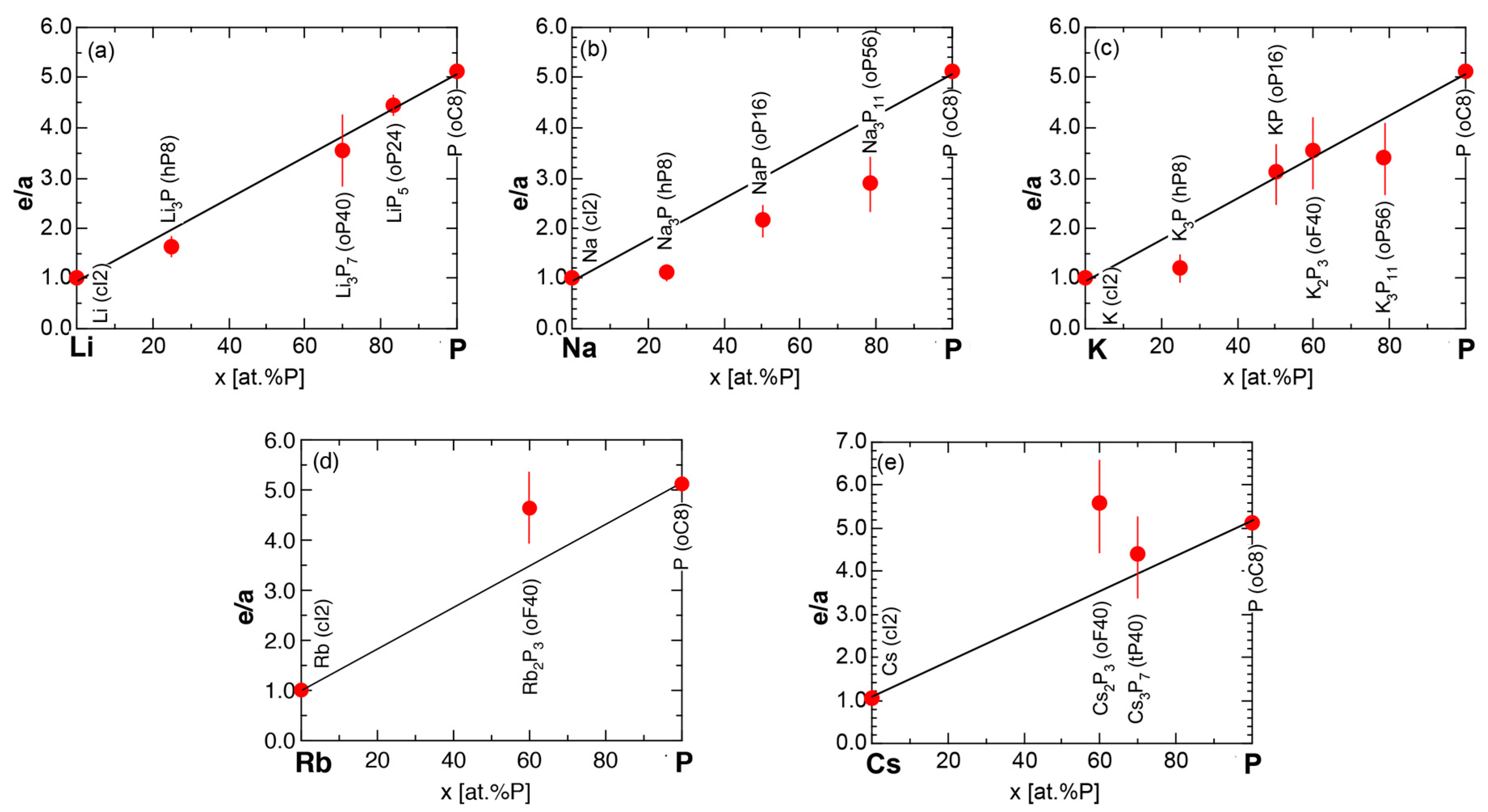
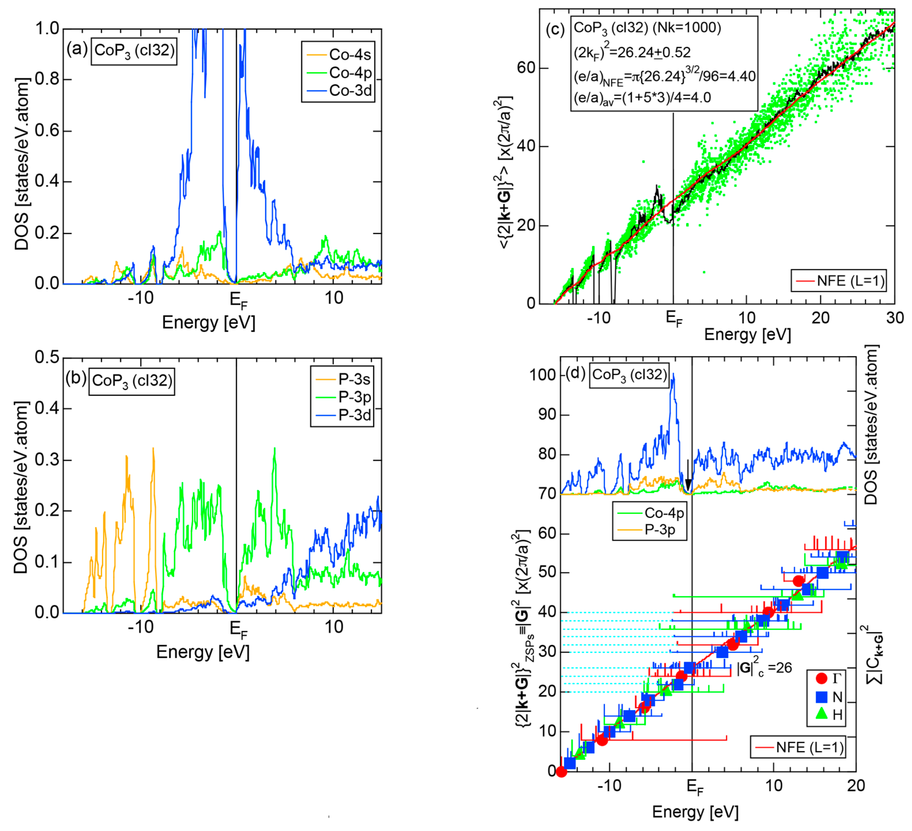
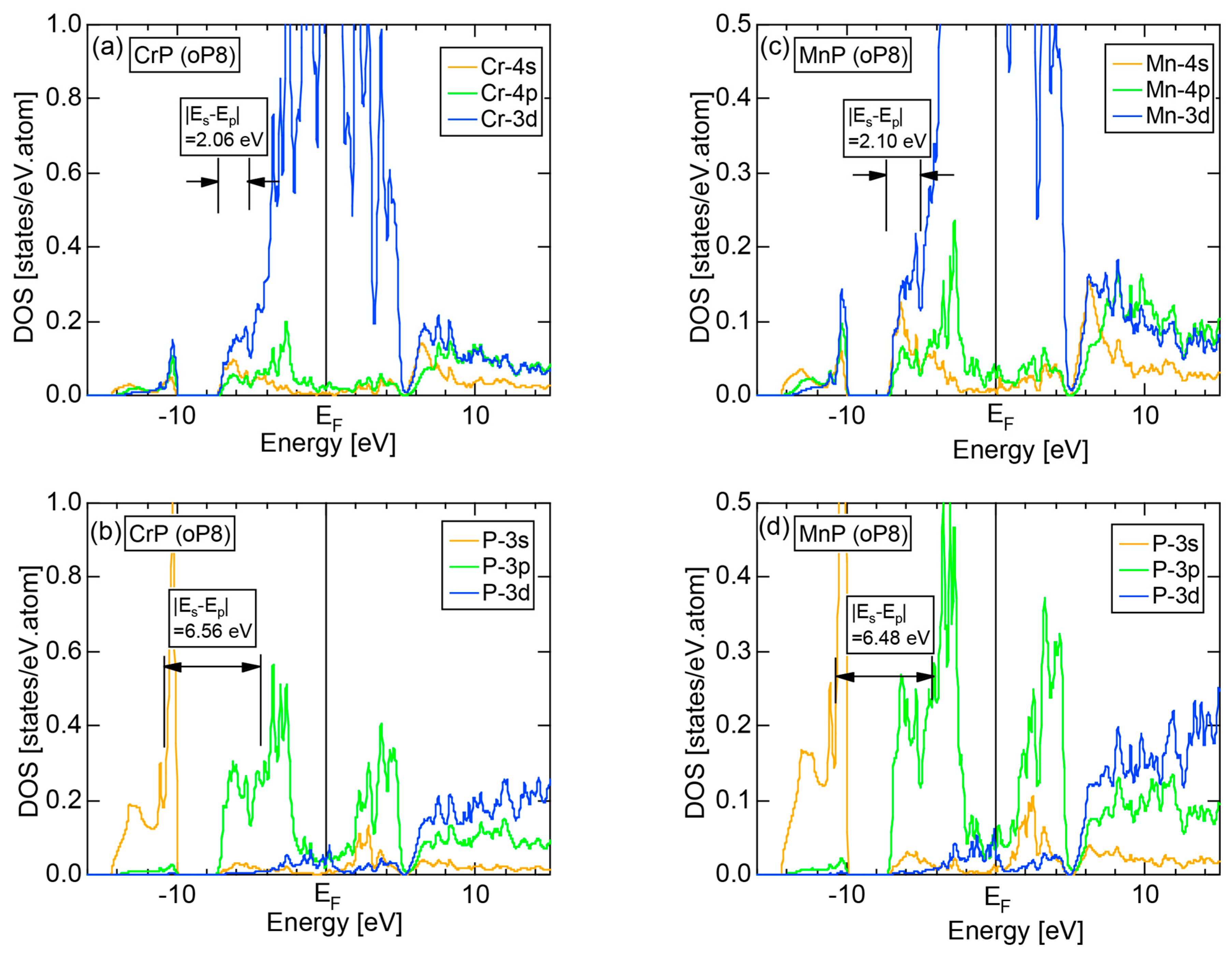
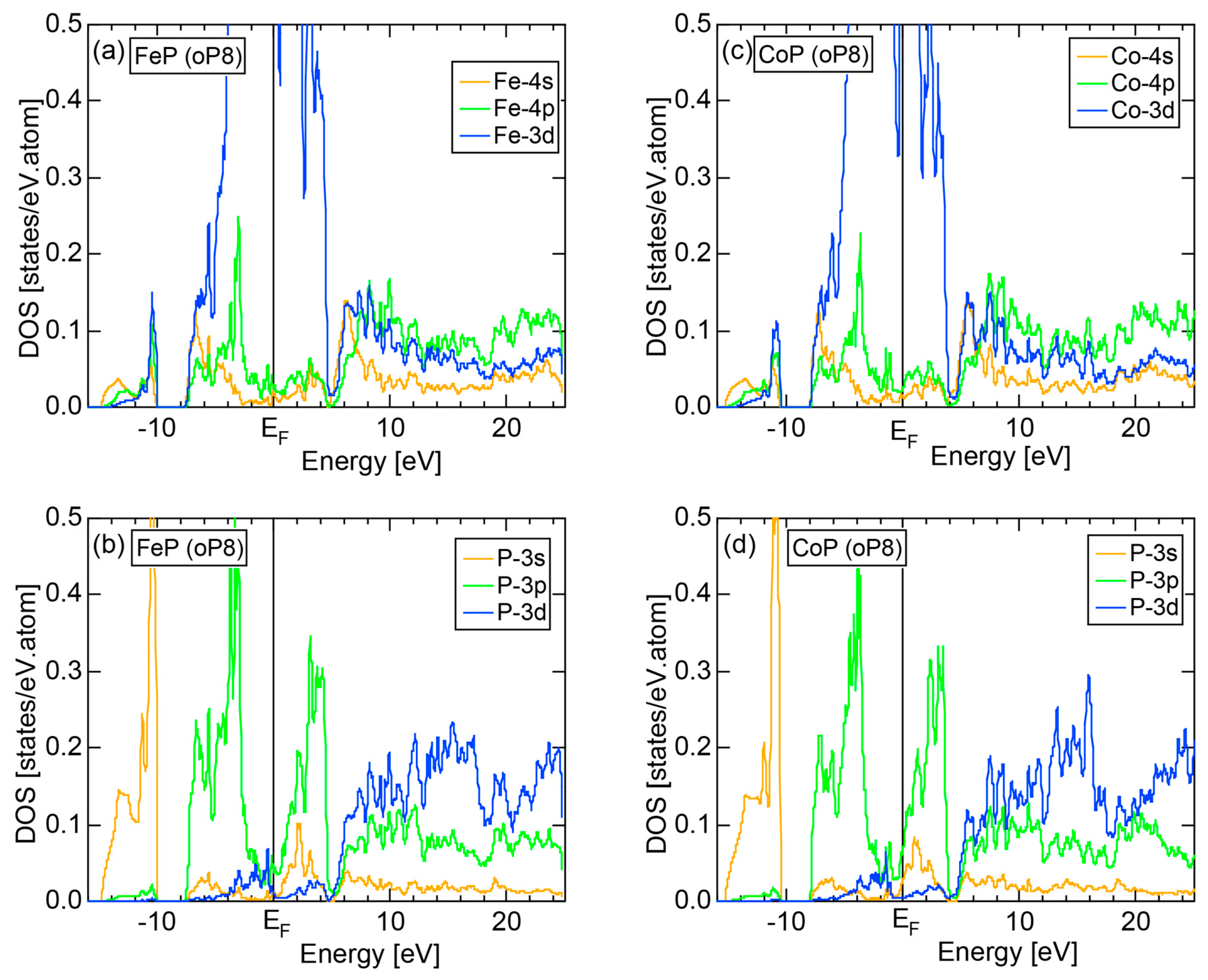
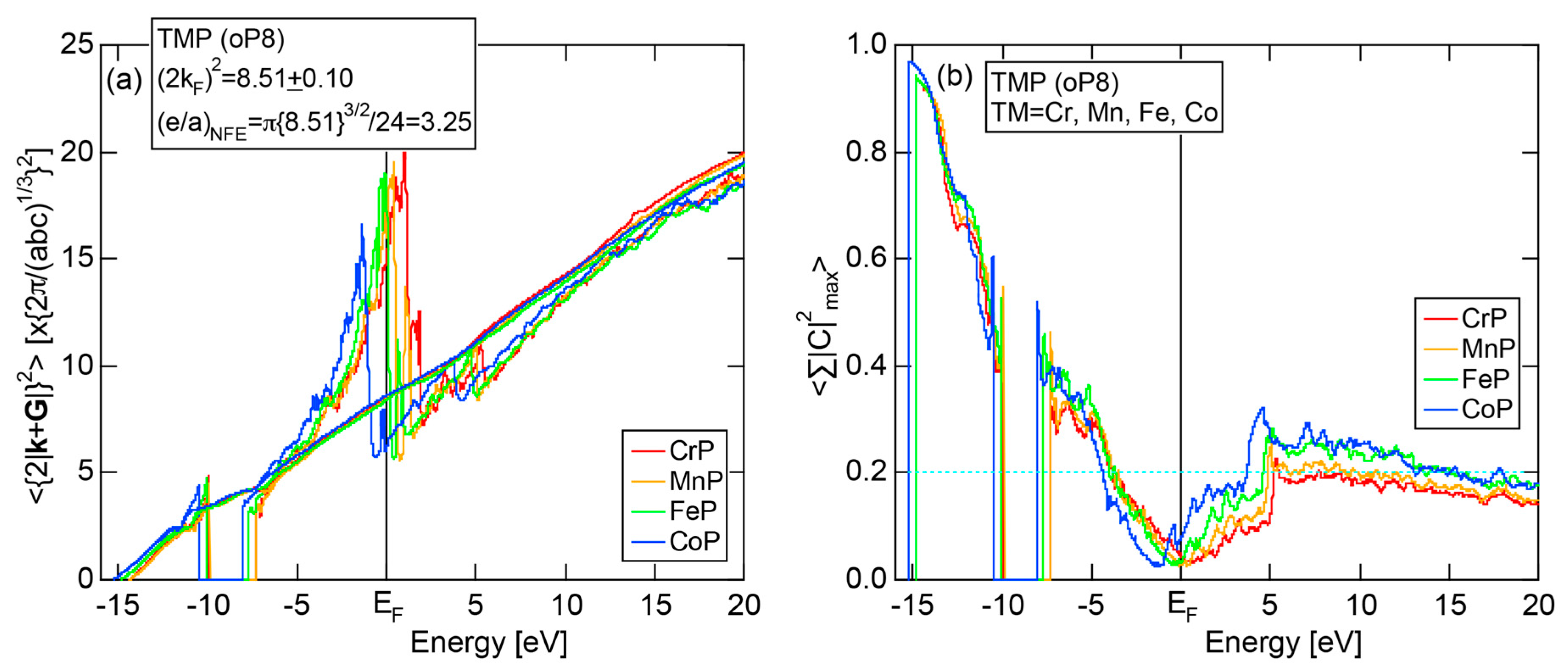
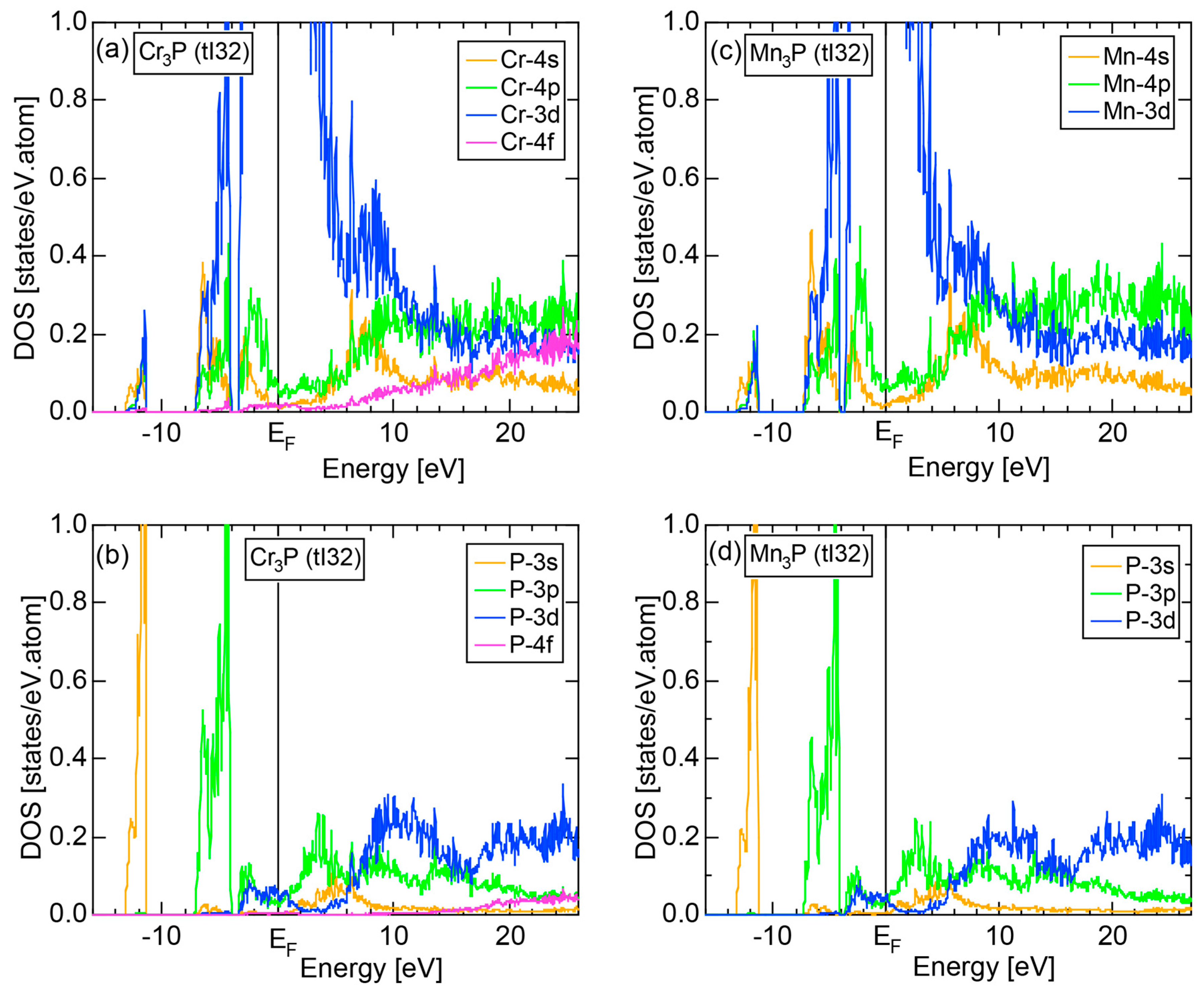
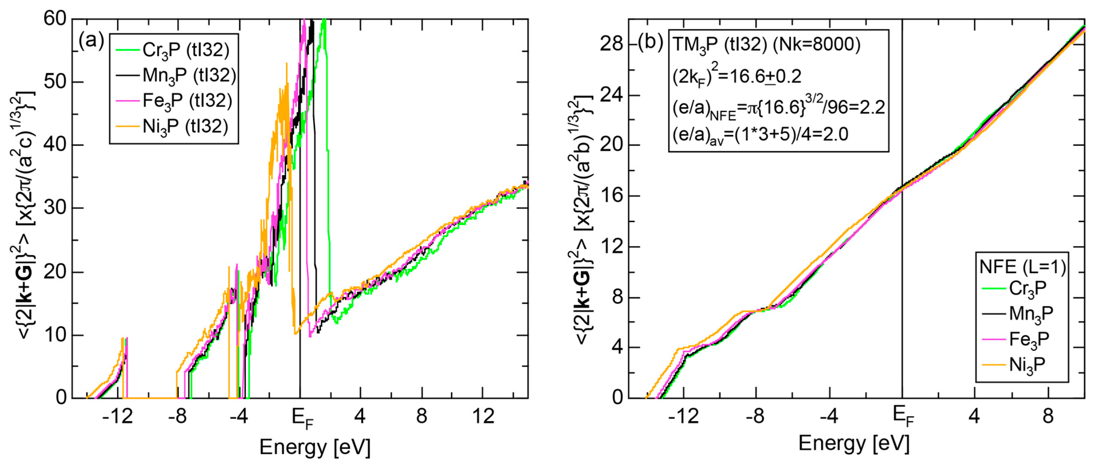
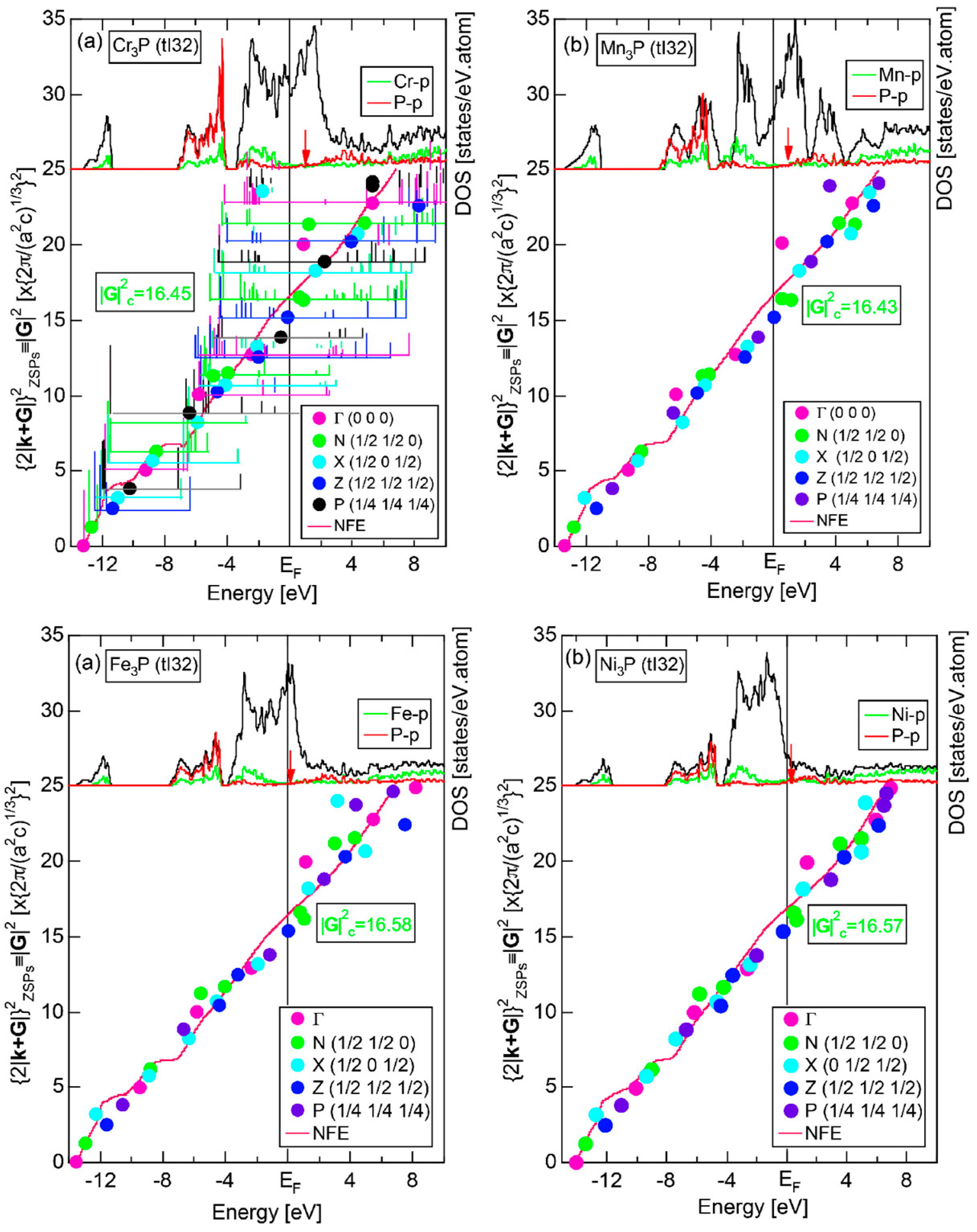
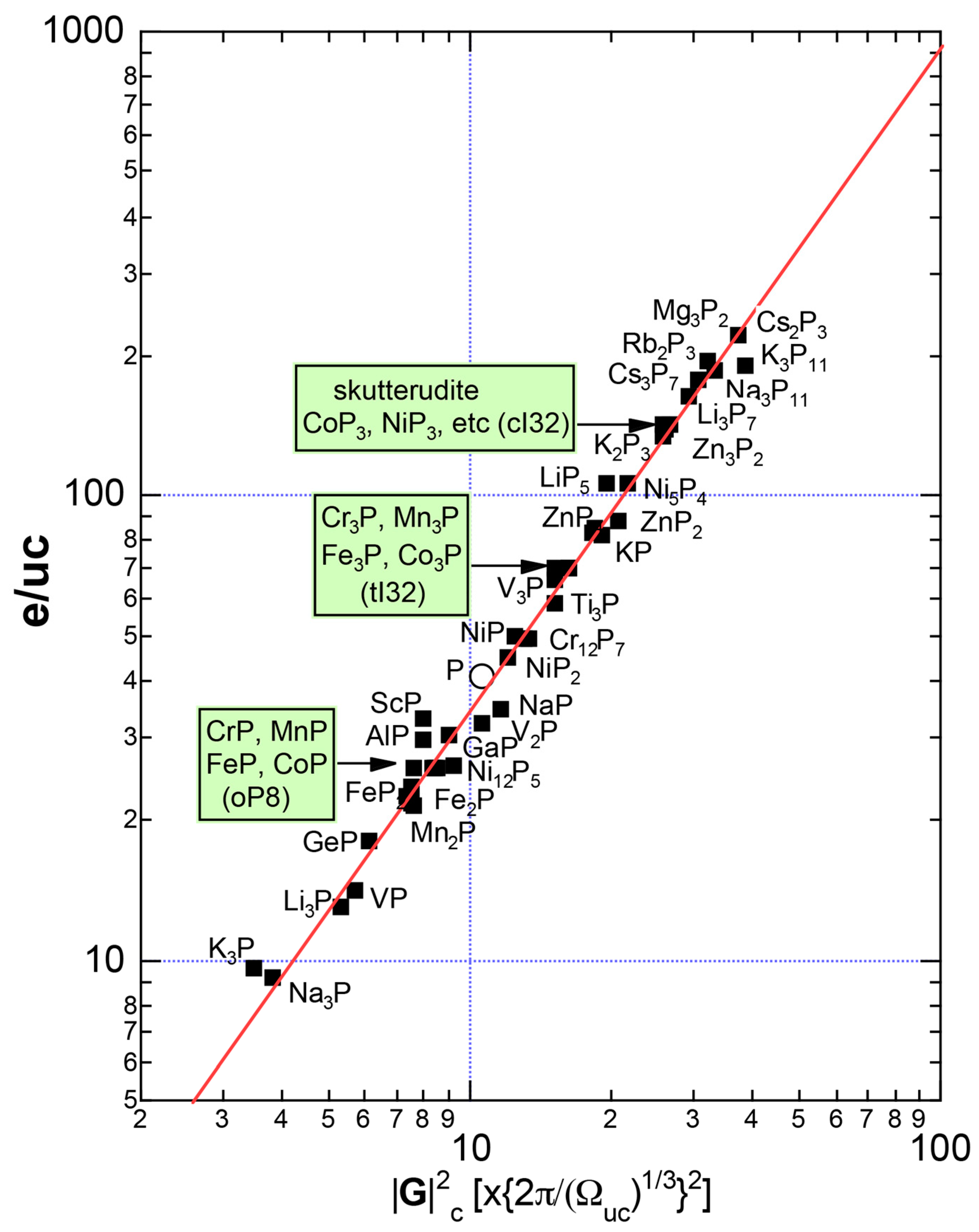
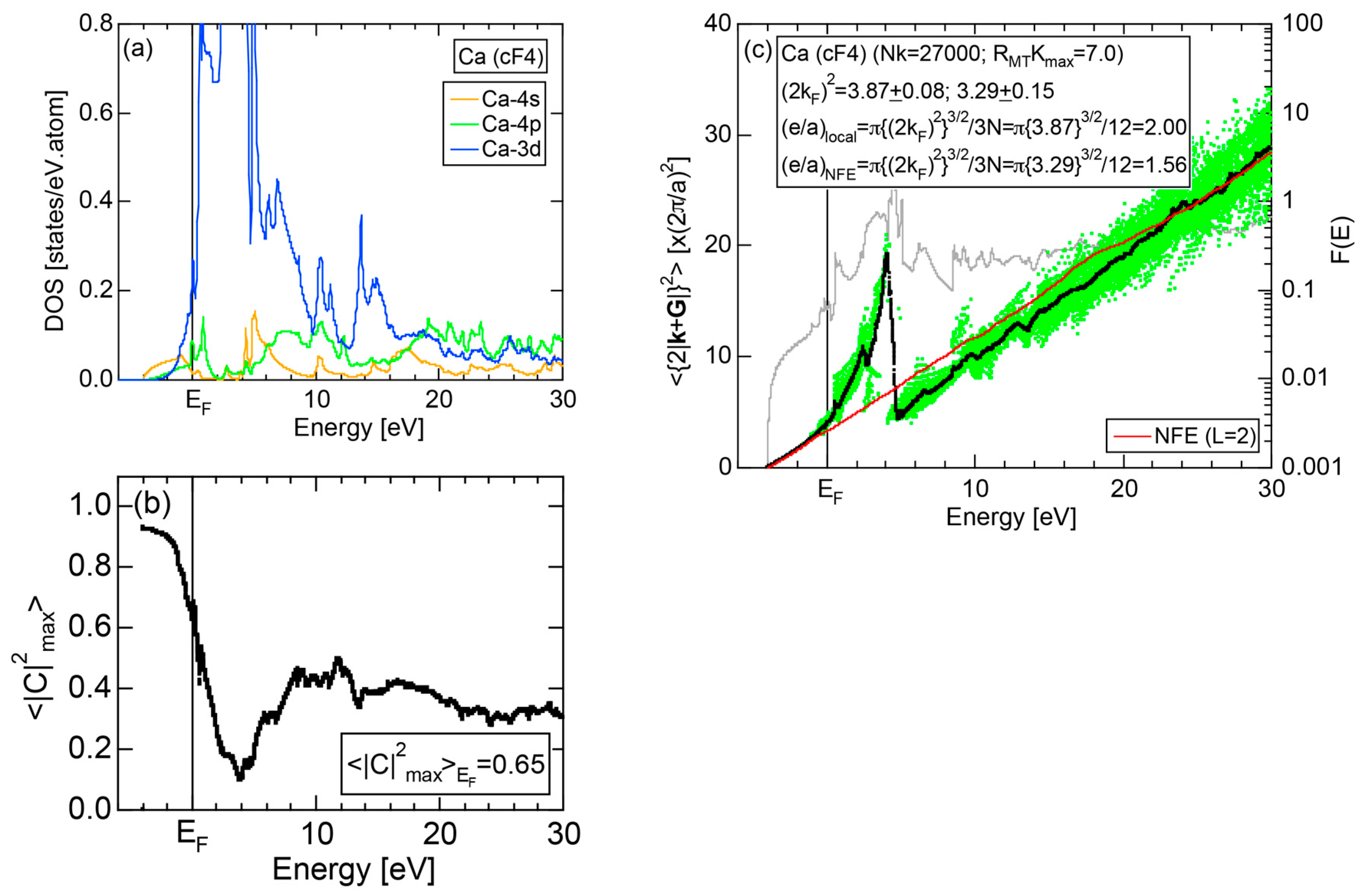
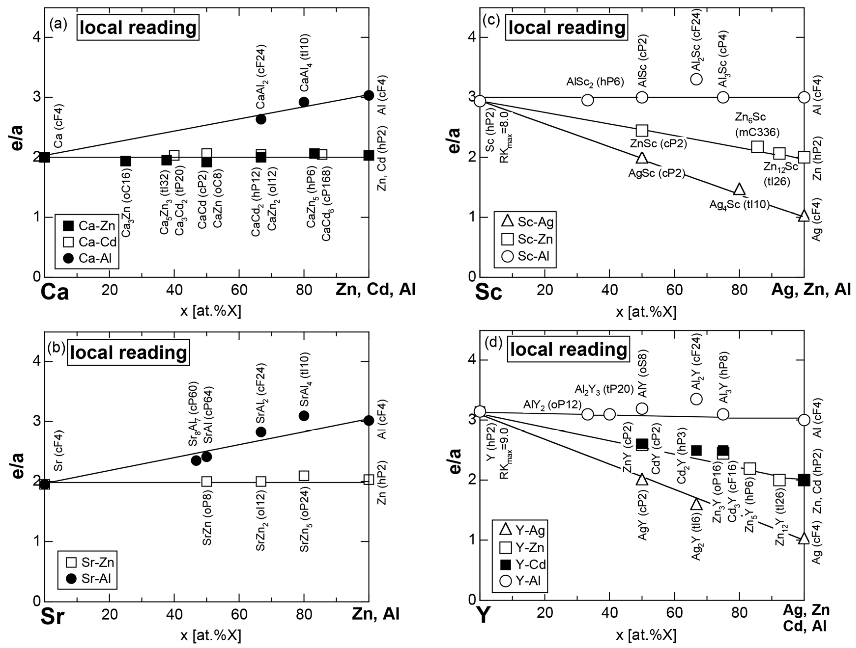
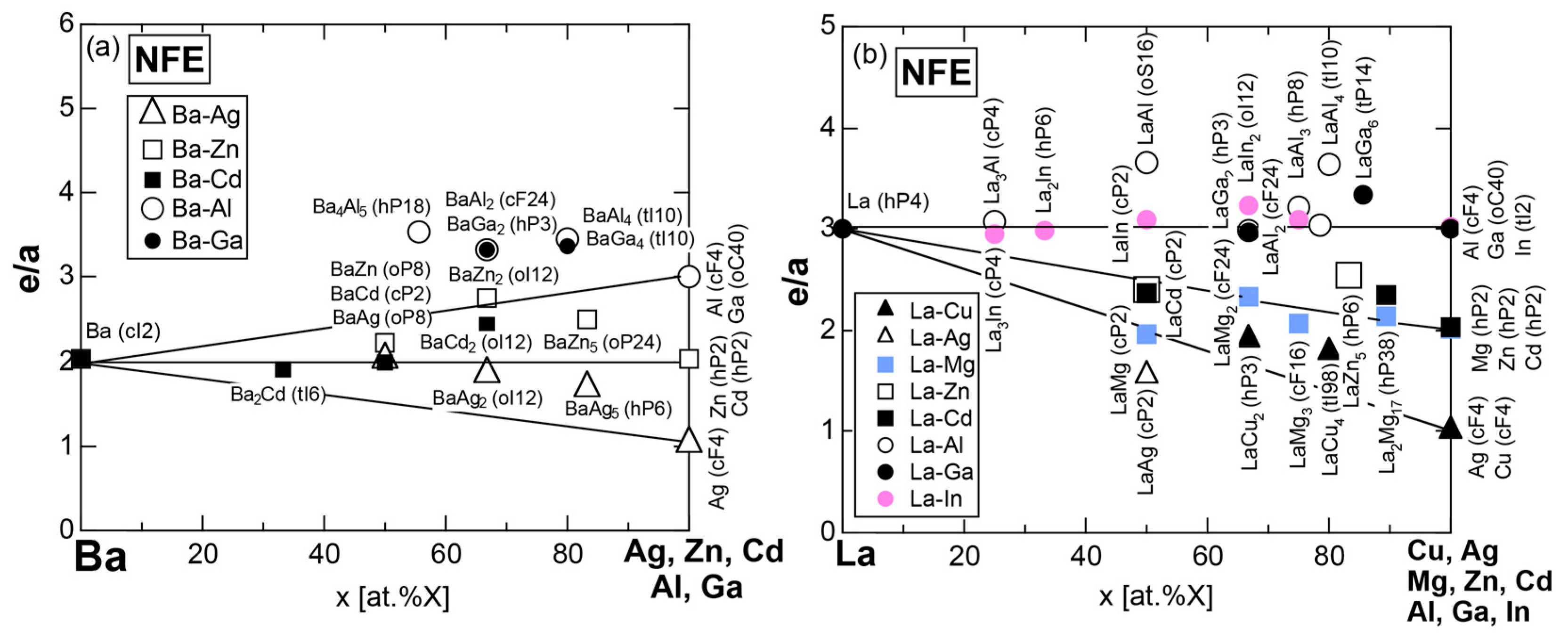
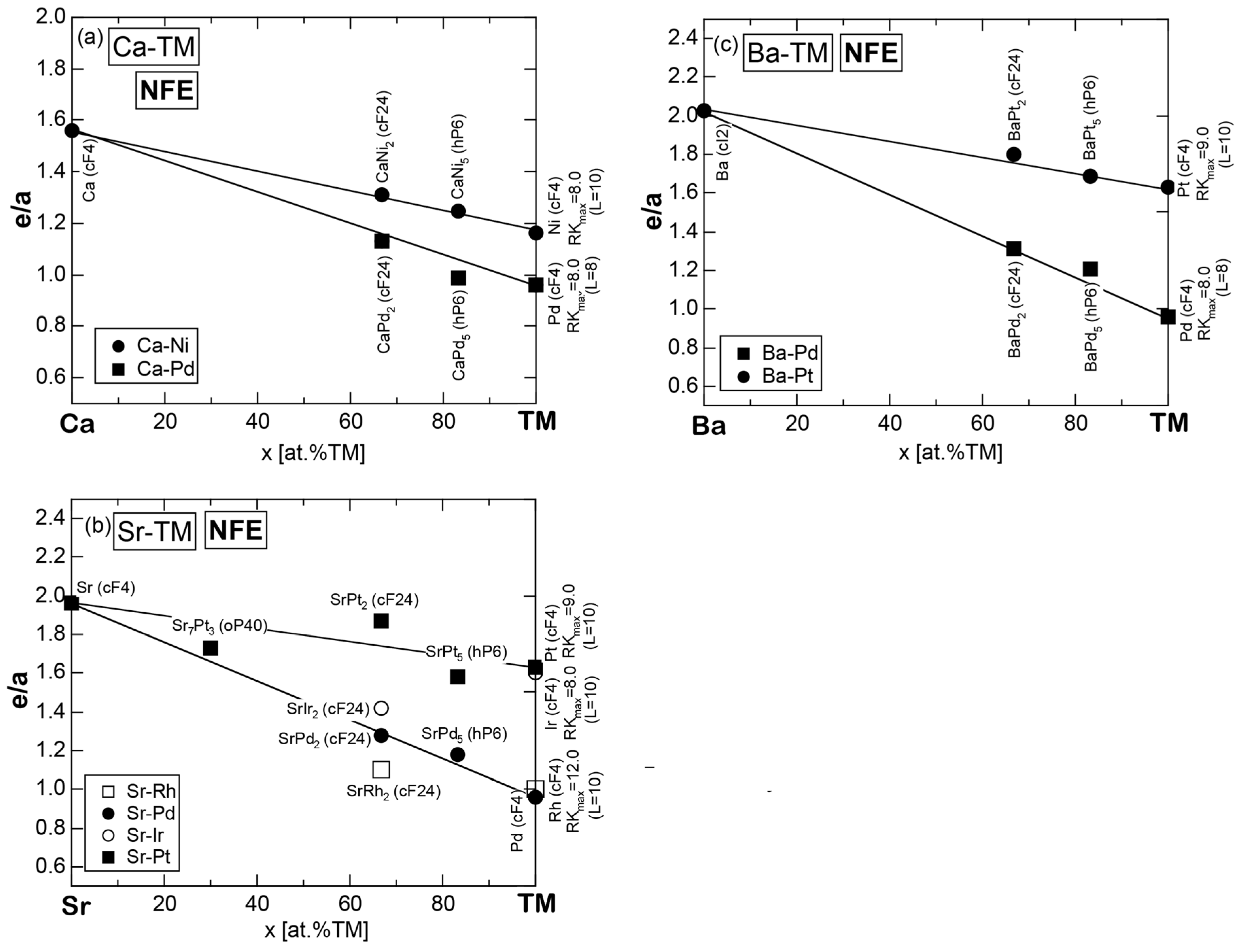
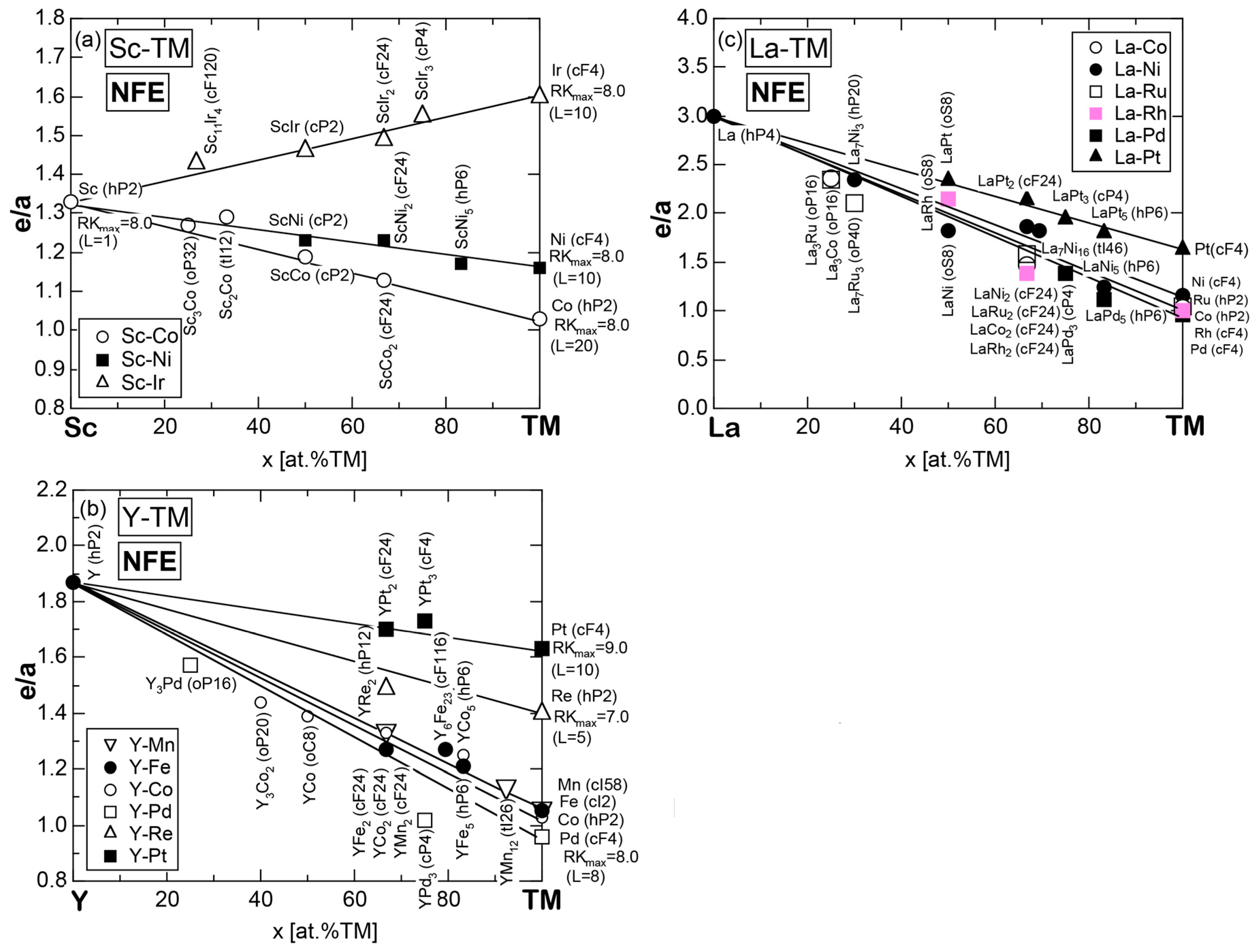
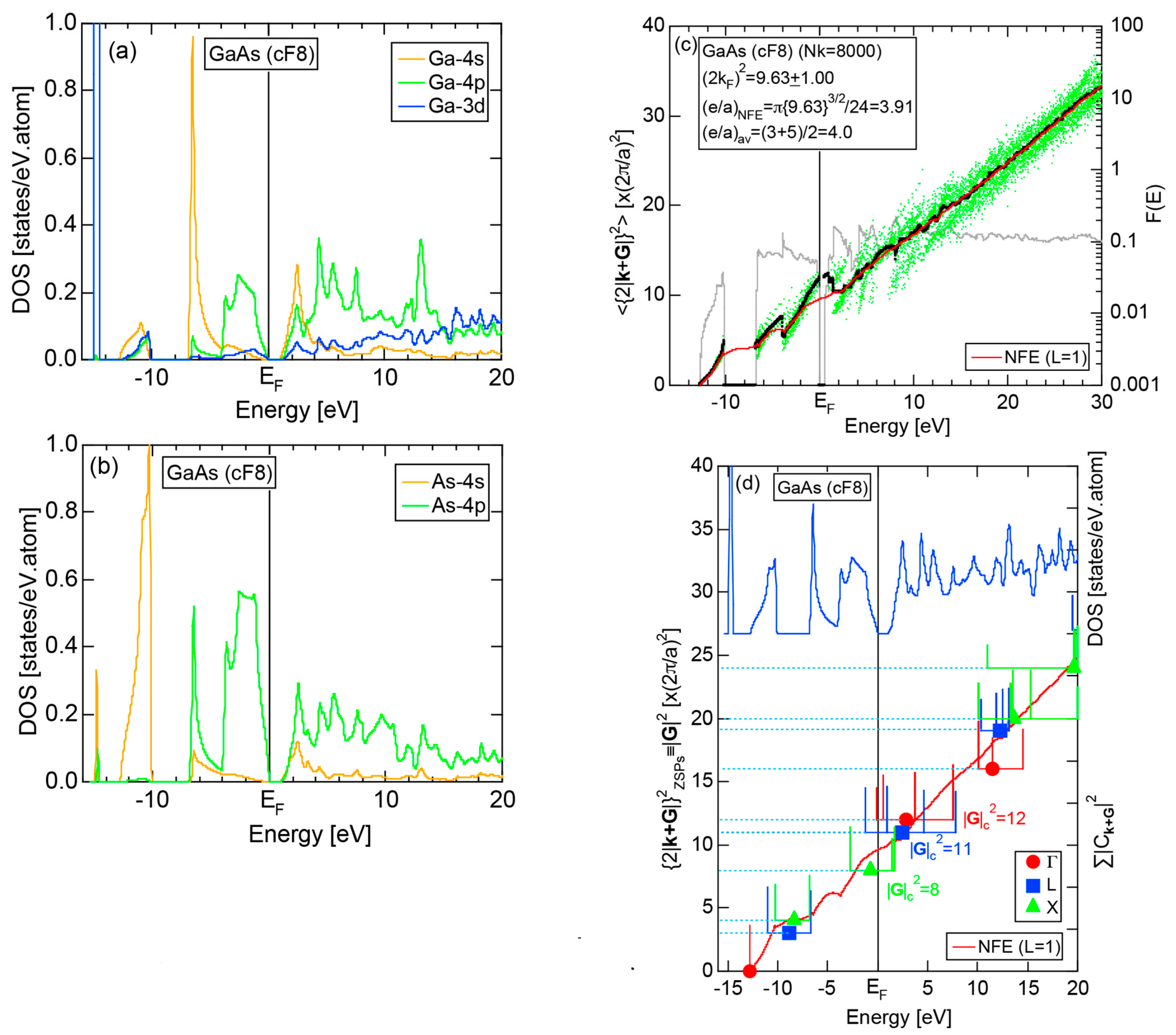
Table 1.
e/a for 54 elements in the periodic table.

Two distinct e/a values are listed for Ca, Sc and Y (See Section 7). The value in the top level is used for the element itself and also when alloyed with non-TM elements. The value in the bottom level is used when alloyed with TM elements.
Table 2.
Allen’s electronegativities of elements in the Periodic Table.

| Subgroup | System | N | (2kF)2 | e/a | e/uc | |G|2c | |
|---|---|---|---|---|---|---|---|
| × (2π/a)2 | × (2π/a)2 | ||||||
| gamma-brasses | 1 | Cu5Zn8 (cI52) | 52 | 18.5 ± 0.1 | 1.60 ± 0.02 | 83 | 18 |
| Ag5Zn8 (cI52) | 52 | 18.5 ± 0.1 | |||||
| Al4Cu9 (cP52) | 52 | 18.5 ± 0.1 | |||||
| In4Ag9 (cP52) | 52 | 18.5 ± 0.1 | |||||
| 2 | Al8V5 (cI52) | 52 | 22.7 ± 1.1 | 2.1 ± 0.1 | 109 | 22 | |
| Al8Cr5 (cI52) | 52 | 22.1 ± 1.1 | |||||
| 3 | Ag5Li8 (cI52) | 52 | 13.51 ± 0.27 | 1.00 ± 0.02 | 52 | 14 |
Table 4.
Hume-Rothery electron concentration rule for RT-type 1/1-1/1-1/1 and 2/1-2/1-2/1 approximants.
| Subgroup | Approximants | Space Group | N | |G|2c × (2π/a)2 | a Å | 2d Å | (2kF)2 × (2π/a)2 | e/a | e/uc | |
|---|---|---|---|---|---|---|---|---|---|---|
| 1/1 | 1 | Al3Mg4Zn3 | Im-3 | 160 | 50 | 14.355 | 4.06 | 49.8 | 2.30 | 368 |
| Al9Mg8Ag3 | Im-3 | 160 | 50 | 14.4799 | 4.09 | 49.4 | 2.27 | 363 | ||
| 2 | Al21Li13Cu6 | Im-3 | 160 | 46 | 13.89 | 4.09 | 47.1 | 2.10 | 336 | |
| Ga21Li13Cu6 | Im-3 | 160 | 46 | 13.568 | 4.00 | 47.6 | 2.15 | 344 | ||
| 3 | Na26Au24Ga30 | Im-3 | 160 | 42 | 14.512 | 4.48 | 41.8 | 1.77 | 283 | |
| Na26Au37Ge18 | Im-3 | 162 | 42 | 14.581 | 4.50 | 41.4 | 1.72 | 278 | ||
| Na26Au37Sn18 | Im-3 | 162 | 42 | 15.009 | 4.63 | 41.1 | 1.70 | 275 | ||
| Na26Cd40Pb6 | Im-3 | 160 | 42 | 15.992 | 4.94 | 42.3 | 1.80 | 288 | ||
| 2/1 | 1 | Al13Mg27Zn45 | Pa-3 | 680 | 126 | 23.0349 | 4.10 | 124.0 | 2.13 | 1448 |
| 2 | Na27Au27Ga31 | Pa-3 | 680 | 110 | 23.446 | 4.47 | 109.2 | 1.76 | 1197 |
| Subgroup | Approximants | Space Group | N | |G|2c × (2π/a)2 | a Å | 2d Å | (2kF)2 × (2π/a)2 | e/a | e/uc | |
|---|---|---|---|---|---|---|---|---|---|---|
| 1/1 | 1 | Al114Mn24 | Pm-3 | 138 | 50 | 12.68 | 3.59 | 48.9 | 2.59 | 357 |
| Al114Re24 | Pm-3 | 138 | 50 | 12.86 | 3.64 | 48.6 | 2.57 | 355 | ||
| Al102Re24Si12 | Pm-3 | 138 | 50 | 12.8603 | 3.64 | 51.0 | 2.76 | 381 | ||
| Al108Cu6Fe24Si6 | Pm-3 | 144 | 50 | 12.48 | 3.53 | 50.0 | 2.57 | 370 | ||
| Al108Cu6Ru24Si6 | Pm-3 | 144 | 50 | 12.6832 | 3.59 | 51.7 | 2.70 | 389 |
| Subgroup | Approximants | Space Group | N | |G|2c × (2π/a)2 | a Å | 2d Å | (2kF)2 × (2π/a)2 | e/a | e/uc | |
|---|---|---|---|---|---|---|---|---|---|---|
| 1/1 | 1 | Zn6Sc | C2/c | 336 | 80 | a = 19.47 b = 13.79 c = 19.55 β = 89.931o | 79.0 ± 0.2 | 2.18 | 732 | |
| Cd6Ca | Pm-3 | 168 | 46 | 15.702 | 4.63 | 47.1 ± 1.0 | 2.01 | 338 | ||
| Cd6Yb | Im-3 | 168 | 46 | 15.638 | 4.61 | 47.5 ± 1.0 | 2.04 | 343 |
| Type | Compounds | Lattice Constant Å | N | |G|2c × (2π/a)2 | (2kF)2 × (2π/a)2 | e/a | e/uc |
|---|---|---|---|---|---|---|---|
| I-III cF32 Fd-3m | LiAl | 6.3757 | 32 | 16 | 16.29 ± 0.20 | 2.09 ± 0.06 | 67 |
| LiGa | 6.150 | 32 | 16 | 15.97 ± 0.20 | |||
| LiIn | 6.7920 | 32 | 16 | 15.75 ± 0.20 | |||
| NaIn | 7.332 | 32 | 16 | 15.99 ± 0.20 | |||
| NaTl | 7.473 | 32 | 16 | 16.12 ± 0.20 | |||
| I-II cF32 Fd-3m | LiZn | 6.209 | 32 | 12 | 13.00 ± 0.20 | 1.53 ± 0.02 | 49 |
| LiCd | 6.702 | 32 | 12 | 13.03 ± 0.20 |
| System | Space Group | Pearson Symbol | |G|2c × (2π/a)2 | (2kF)2 × (2π/a)2 | e/a | e/uc |
|---|---|---|---|---|---|---|
| P | Cmca | oC8 | 10.56 | 11.30 ± 0.33 | 4.97 | 40 |
| As | R-3m | hR2 | 4.74 | 4.45 ± 0.22 | 4.92 | 10 |
| Sb | R-3m | hR2 | 4.54 | 4.49 ± 0.22 | 4.99 | 10 |
| Bi | R-3m | hR2 | 4.53 | 4.46 ± 0.22 | 4.94 | 10 |
Table 9.
Phosphorus-based isostructural compounds obeying the Hume-Rothery electron concentration rule
| Family | Subgroup | System | N | |G|2c × [2π/(Ωuc)1/3]2 | (2kF)2 × (2π/a)2 | e/a | e/uc |
|---|---|---|---|---|---|---|---|
| skutterudites (TM)M3 (TM = Co, Rh, Ir, Ni) (M = P, As, Sb) | 1 | CoAs3 (cI32) | 32 | 26 | 25.2 ± 0.2 | 4.34 ± 0.20 | 139 |
| RhAs3 (cI32) | 32 | 26 | 26.3 ± 0.2 | ||||
| IrAs3 (cI32) | 32 | 26 | 26.7 ± 0.2 | ||||
| CoSb3 (cI32) | 32 | 26 | 26.5 ± 0.2 | ||||
| RhSb3 (cI32) | 32 | 26 | 27.3 ± 0.2 | ||||
| IrSb3 (cI32) | 32 | 26 | 27.8 ± 0.2 | ||||
| NiP3 (cI32) | 32 | 26 | 25.1 ± 0.2 | ||||
| CoP3 (cI32) | 32 | 26 | 25.0 ± 0.2 | ||||
| RhP3 (cI32) | 32 | 26 | 25.9 ± 0.2 | ||||
| IrP3 (cI32) | 32 | 26 | 26.7 ± 0.2 | ||||
| (TM)P (TM = Cr, Mn, Fe, Co) | 1 | CrP (oP8) | 8 | 8.38 | 8.53 ± 0.43 | 3.25 ± 0.05 | 26 |
| MnP (oP8) | 8 | 8.49 | 8.47 ± 0.42 | ||||
| FeP (oP8) | 8 | 8.56 | 8.41 ± 0.42 | ||||
| CoP (oP8) | 8 | 8.29 | 8.60 ± 0.83 | ||||
| (TM)3P (TM = Cr, Mn, Fe, Ni) | 1 | Cr3P (tI32) | 32 | 16.3 | 16.67 ± 0.83 | 2.20 ± 0.05 | 70 |
| Mn3P (tI32) | 32 | 16.4 | 16.67 ± 0.83 | ||||
| Fe3P (tI32) | 32 | 16.2 | 16.47 ± 0.83 | ||||
| Ni3P (tI32) | 32 | 16.2 | 16.56 ± 0.33 |
| Compounds | Pearson Symbol | Energy Gap (eV) | (2kF)2 × (2π/a)2 | e/a | (e/a)av |
|---|---|---|---|---|---|
| SiP | oC48 | 1.2 | 35.2 | 4.55 | 4.56 |
| GeP | tI4 | pseudogap | 6.66 | 4.50 | 4.56 |
| ScP | cF8 | pseudogap | 10.02 | 4.15 | 4.03 |
| TiP2 | oP12 | pseudogap | 13.19 | 4.18 | 3.72 |
| VP2 | mC12 | pseudogap | 13.16 | 4.17 | 3.75 |
| CrP2 | mC12 | pseudogap | 12.55 | 3.88 | 3.72 |
| MnP4 | aP10 | 0.4 | 12.25 | 4.49 | 4.31 |
| CoP3 | cI32 | pseudogap | 26.24 | 4.2 | 4.12 |
| NiP3 | cI32 | pseudogap | 26.17 | 4.2 | 4.13 |
| CuP2 | mP12 | 0.84 | 12.59 | 3.9 | 3.75 |
| Cu2P7 | mC72 | 0.61 | 46.15 | 4.56 | 4.20 |
| Compounds | Pearson Symbol | Energy Gap (eV) | (2kF)2 × (2π/a)2 | e/a | (e/a)av |
|---|---|---|---|---|---|
| ZnP2 | mP24 | pseudogap | 21.47 | 4.34 | 4.0 |
| ZnP2 | tP24 | 1.63 | 19.28 | 3.69 | 4.0 |
| ZnP4 | tP20 | 0.63 | 18.7 | 4.24 | 4.4 |
| Mg3P2 | cI80 | 1.6 | 32.68 | 2.45 | 3.2 |
| MgP4 | mP10 | 0.50 | 11.65 | 4.16 | 4.4 |
| Ca5P8 | mC26 | 1.13 | 20.79 | 3.82 | 3.85 |
| CaP3 | aP8 | pseudogap | 10.7 | 4.58 | 4.25 |
© 2017 by the authors; licensee MDPI, Basel, Switzerland. This article is an open access article distributed under the terms and conditions of the Creative Commons Attribution (CC-BY) license (http://creativecommons.org/licenses/by/4.0/).
Share and Cite
MDPI and ACS Style
Mizutani, U.; Sato, H. The Physics of the Hume-Rothery Electron Concentration Rule. Crystals 2017, 7, 9. https://doi.org/10.3390/cryst7010009
AMA Style
Mizutani U, Sato H. The Physics of the Hume-Rothery Electron Concentration Rule. Crystals. 2017; 7(1):9. https://doi.org/10.3390/cryst7010009
Chicago/Turabian StyleMizutani, Uichiro, and Hirokazu Sato. 2017. "The Physics of the Hume-Rothery Electron Concentration Rule" Crystals 7, no. 1: 9. https://doi.org/10.3390/cryst7010009
Note that from the first issue of 2016, this journal uses article numbers instead of page numbers. See further details here.