
Methods for Calculating Empires in Quasicrystals


Quantum Gravity Research, Los Angeles, CA 90290, USA
*
Author to whom correspondence should be addressed.
Crystals 2017, 7(10), 304; https://doi.org/10.3390/cryst7100304
Submission received: 31 August 2017
/
Revised: 26 September 2017
/
Accepted: 29 September 2017
/
Published: 9 October 2017
(This article belongs to the Special Issue Structure and Properties of Quasicrystalline Materials)
Abstract
:This paper reviews the empire problem for quasiperiodic tilings and the existing methods for generating the empires of the vertex configurations in quasicrystals, while introducing a new and more efficient method based on the cut-and-project technique. Using Penrose tiling as an example, this method finds the forced tiles with the restrictions in the high dimensional lattice (the mother lattice) that can be cut-and-projected into the lower dimensional quasicrystal. We compare our method to the two existing methods, namely one method that uses the algorithm of the Fibonacci chain to force the Ammann bars in order to find the forced tiles of an empire and the method that follows the work of N.G. de Bruijn on constructing a Penrose tiling as the dual to a pentagrid. This new method is not only conceptually simple and clear, but it also allows us to calculate the empires of the vertex configurations in a defected quasicrystal by reversing the configuration of the quasicrystal to its higher dimensional lattice, where we then apply the restrictions. These advantages may provide a key guiding principle for phason dynamics and an important tool for self error-correction in quasicrystal growth.
1. Introduction—What Is the Empire Problem?
When compared with regular crystals, quasicrystals present more complex structures and variations and have dynamic patterns that can be non-local due to the non-local nature of the quasicrystal itself [1]. Although not obvious, it is true that a given local patch of tiles in a quasicrystal can force tiles to lie in non-adjacent (non-local) positions. This set of tiles, which are forced by a given vertex type, or in this paper extended to any local patch of tiling, represents the empire of the local patch in the quasicrystal [2], a term originally coined by Conway [3]. The problem of finding these forced tiles for a certain configuration of a quasicrystal [4] is referred to as the empire problem in this paper. Local matching rules serve as a tool to grow an infinite tiling by constraining the way neighboring tiles can join together. However, these local rules tend to result in deception and/or “holes” or “dead surfaces” and therefore cannot grow an infinite perfect quasicrystal [5]. Non-local information is needed to guide a perfect growth of an infinite quasicrystal and its dynamics. The empires of the quasicrystals contain this non-local information and therefore can in principle be used as generators of quasicrystals. Mastering the efficient method of obtaining the empires is thus important for modeling the quasicrystal growth and phason dynamics in quasicrystals.
In this paper, we discuss three methods for generating the empires of the vertex configurations in quasicrystals, using Penrose tiling as an example. In Section 2, we calculate the empires of the simplest one dimensional quasicrystal, the Fibonacci chain, using the legal matching rules between local tiles. Then we demonstrate how to obtain the empires of a 2D quasicrystal, Penrose tiling, using the empires of this 1D Fibonacci chain. This method was first introduced in [2] and named the Fibonacci chain method in this paper. In Section 3, we review the multigrid method for generating the empires of the Penrose tiling [4]. Based on the cut-and-project technique [6,7], we introduce a new method for calculating the empires of quasicrystals of any dimension in Section 4 and we compare it with the previous methods in Section 5. In Section 6, we present our conclusions and outlook.
2. The Fibonacci-Grid Method
The empire problem, the problem of finding out which tiles are forced given an initial set of tiles, was first explored by analyzing Ammann bars, a decoration for Penrose tiles realized as a network of five sets of parallel lines. This method was extended by Minnick [8]. Due to the fact that it uses the empire of the Ammann bars, which is in fact a Fibonacci pentagrid [9] of the Penrose tiling, we name the method used in this case the Fibonacci-grid method.
The prolate and oblate rhombuses in Penrose tiling can be decorated using line segments as shown in Figure 1. When two tiles meet along an edge, the line segments from one tile meet the segments from the other at straight angles, forming extended lines which are called the Ammann bars [2]. These matching rules using the Ammann bars are equivalent to the single- and double-arrow matching rules for Penrose tiling.
When looking at a large enough Penrose tiling, the Ammann bars extend to form lines which crisscross the plane in a very structured way, as shown in Figure 2. These lines can be grouped together to form five distinct families of parallel lines called , where each grid consists of lines normal to one of the following five vectors , where . The gaps between neighboring parallel lines are represented by two values, a “long” gap L and a “short” gap S, where the ratio between these two distances is the golden ratio . The gaps for a particular grid from a sequence of long and short gaps, denoted by a sequence of L’s and S’s.
These sequences turn out to be Fibonacci chains, or Fibonacci words, which represent the simplest one dimensional quasicrystals and which can be generated by the following iterative process. Let us start with the two words and and let be the concatenation of the previous two words. The infinite Fibonacci word is defined to be the limit . Alternatively, one can start with and apply the following substitution rules to iterate one word to the next .
The rules for creating the infinite Fibonacci word prohibit the formation of certain sub-words. For instance, there cannot be three consecutive L’s appearing in nor can there be two S’s next to each other. So and are not valid Fibonacci chains, and if one has then the next letter must be S. Likewise an S must always be followed by an L.
Since the Penrose tiling is indeed a network of these Fibonacci words, calculating the empires in the Fibonacci words will directly lead us to the empires of the Penrose tiling.
Given an initial sub-word, W, one can identify its empires, which consists of all the letters that are forced by the presence of W. For example, the word (shown in red) has the following empire (shown in blue):
While there is some freedom in choosing letters for the gaps in the empires, there is no freedom in choosing letters at positions shown in blue. Whenever an is present in a Fibonacci chain, the 13th letter following the is forced to be an and the 19th letter is forced to be an . The empires extend to include an infinite number of letters.
We can apply this method to the Ammann bars, with the purpose of finding the empires in Penrose tiling. For a given patch of tiles , where n is the number of tiles in T, there will be some Ammann bars (from the same or from different parallel line sets) running through P. Within each parallel line set i, the bars are separated with long and/or short gaps between them forming the given initial word , where . The empires associated with each can be thus calculated and as a result, all other forced Ammann bars within the same grid can be found.
An example is shown in Figure 3, where the given patch at the center is colored red, the associated bars are colored green and the empire or forced bars are colored blue. A tile or a small cluster of tiles is forced where the Ammann lines intersect in a certain configuration. Detailed rules are discussed in [8]. As a result, the first set of the forced tiles are determined (colored blue in Figure 3). As the first set of forced tiles are decided, more Ammann bars (colored red in Figure 3) can be forced by these tiles, which in turn will force other tiles, as a result of the intersection of the red bars with other red or blue bars, as shown in Figure 3. For solving the empire problem, this approach is workable but tedious, therefore impractical in modeling the growth or dynamics of quasicrystals.
3. The Multigrid Method
The multigrid method offers a robust algorithm for generating quasicrystalline tilings or quasicrystals of Euclidean space as well as the empires of the quasicrystals. A multigrid is the superposition of distinct grids. A grid is a family of parallel hyperplanes. A grid with an equal spacing between hyperplanes can be expressed as a countable union of hyperplanes which are all normal to a non-zero grid vector :
where each hyperplane is indexed by an integer and the quantity provides a shift of the grid away from the origin. The distance between neighboring hyperplanes is equal to .
A tiling of can be constructed by taking the dual of the multigrid, meaning a point where m hyperplanes intersect in the multigrid space will correspond to a -sided polytope in the tiling space, with opposite sides being parallel [10].
For constructing a Penrose tiling in , the pentagrid, a multigrid consisting of five grids is used.
We define a pentagrid as a set of five grids in the plane (Figure 4) for , where each grid has an associated unit-length grid vector and shift (Figure 5), but rather than indexing the grids using the integers, we use the half-integers instead .
The quantities form a 5-tuple called the shift vector . They satisfy condition to obtain the true Penrose tiling, which obeys the Penrose matching rules. Let the multigrid denote the superposition of all grids for a given shift vector and let be the tiling of which is dual to . It is important to choose so that the pentagrid is nonsingular and no more than two grid lines intersect at a given point [6]. This can be achieved by choosing only the rational and non-complimentary distinct values for . This restriction ensures that consists only of rhombuses. The dualizing procedure is shown in Figure 6.
Each grid divides the plane into open strips, , which lay between neighboring grid lines (Figure 7a).
Each region is constant with respect to the function , where the right-hand term denotes the rounding function returning the nearest integer. Each strip can be rewritten as (the open interior of) the preimage of k under .
The open regions of the plane between the grid lines are called meshes, which correspond to vertices in the dual. For a point , which is not located on any of the grid lines, the mesh region (Figure 7b) that contains can be expressed as the intersection of the five strips, which contain , namely (where ). If represents the 5-tuple , then the mesh can be written as the interior of the preimage .
In this way, each mesh M can be identified with the point , where is equal to for arbitrary choice of .
To associate a point on the plane with each mesh, we use the linear transformation , defined by taking the linear combination of grid vectors with coefficients . This can be written in matrix form as , where is the matrix with column vectors .
Given two grid lines and , let denote their intersection point, as shown in Figure 7c.
The point represents a rhombus in the dual tiling . The four vertices of this rhombus correspond to the mesh regions adjacent to which are indexed by four 5-tuples (Figure 7c), where and are the standard basis vectors for . After applying the transformation , the vertices of tile T can be written as points in the plane: .
We can write to indicate the tile which is dual to the point at the intersection of the two grid lines and . When the shift vector is perturbed to a new value, , the grid lines change position and the location of the intersection changes accordingly. A tile remains included in the dual tiling associated to the new shift vector as long as has the same value, as long as remains within the same three strips for . The three conditions for provide the constraints necessary to keep included in the dual tiling . The constraints are equivalent to the linear inequalities:
where and are given by the simultaneous solution to the equations:
These equations can be rewritten in matrix notation. Let be the matrix with column vectors and . For the vectors and are non-collinear and the matrix is non-degenerate, with the inverse . The intersection can be written in terms of and . Again, for convenience we use .
The dot product can be expressed as:
The inequalities can be expressed in terms of and :
To simplify the algebra, we define the linear functions [4] for and :
The functions can be expressed in terms of the indices and .
The inequality can be rewritten as:
For a given tile , these inequalities define a region of suitable shift vectors so that for any , the tile is included in the tiling .
For Penrose tiling, another restriction on is imposed by the sum condition, , which N. G. de Bruijn [11] has shown to be a necessary condition that ensures that the tiling obeys the matching rules. Consequently, we add the following as a further restriction which defines [11].
For a collection of tiles let denote the mutual intersection of all the regions .
We define the empire to be the set of tiles T for which contains . Indeed, for any it is true that , and if for some tile T, then it is also true that , implying that .
In order to compute , a linear program can be employed. Each tile gives three inequalities for . We collect all the linear inequalities given by all tiles and add to this list the sum condition as a linear equality. This list provides the linear constraints that define , which are to be used in the linear program.
We use each function as an objective function in the linear program in order to find the minimum and maximum values that achieves on . Let and be the values obtained from the linear program.
A tile is included in the empire if and only if:
Figure 8 shows a sample result of the empire calculation for two different local vertex types in Penrose tiling, one with 5-fold symmetry and one without. The green tiles are the forced tiles that belong to the empire of the local vertex configuration (red), while the blue tiles are not forced. Figure 9 shows the empire of the rest of local vertex types in Penrose tiling. Notice that the density of the empires differs for different vertex types and one of the empires is completely empty. Mathematically, the density of the empire is determined by the volume of the empire-window. For example, the empire-window of the vertex type shown in Figure 8a is too narrow to capture any other tiles in it, therefore the empire is empty. The density of the empires is also related to the frequency of the vertex types [12] so that more frequent vertex types have lower empire densities.
The multigrid method is relatively simpler and faster when compared with the Fibonacci-grid method, but might not be practical in cases where there is not an obvious simple dual grid for the quasicrystal. Also, when there is a defect in the quasicrystal, this method will no longer work because the dual of the quasicrystal in this case will no longer be a perfect multigrid. However, we discovered a new method, named the cut-and-project method, that solves these issues. Details about this method will be discussed in the following section.
4. The Cut-and-Project Method
The cut-and-project technique for generating quasiperiodic tilings from a higher dimensional lattice is well developed [7]. For a regular lattice and lattice point , let denote the Voronoi cell centered at .
For a regular lattice, the Voronoi cells for each lattice point are identical up to translation, so let denote the generic Voronoi cell for the origin and let denote the translation , where .
Let E be a totally irrational [7] m-dimensional affine subspace, for , where is a linear subspace and E is the translation of V by the shift vector and let be the orthogonal projection onto E. A quasicrystalline tiling of E can be generated by taking the projected points for all lattice points with Voronoi cells intersecting E non-trivially, , as shown in Figure 10a. This higher dimensional lattice is called the mother lattice of the quasicrystalline tiling in the lower dimension.
If two points are neighboring vertices in the lattice (sharing a common lattice edge), then the projected points and are to be connected by an edge as well.
The Voronoi cell centered at , , intersects E if and only if the translation of the Voronoi cell, centered at includes the lattice point (this follows from the definition of the Voronoi cell and the fact that is the point of E that is closest to ). Let be the orthogonal complement of E and let be the projection onto . If , then . Conversely, if , then there is some translation , where such that contains , in which case contains and so does intersect E.
The orthogonal projection of onto is called the cut-window, (Figure 11). A lattice point is included in the tiling if and only if , as shown in Figure 10b.
To construct a Penrose tiling, let be the lattice , be the plane with the basis
and be the translation of V away from the origin.
For the orthogonal space , we choose the basis as follows:
The projection is given by the matrix and the linear map into the orthogonal space is given by the matrix .
The Voronoi cell at the origin is a unit 5-cube with 32 vertices . The 5-dimensional volume contained within projects to a 3-dimensional volume in , which is computed as the convex hull of the point set . This describes the cut-window and it has the form of a rhombic-icosidodecahedron with 32 vertices and 20 rhombic faces.
The 3-dimensional volume contained within is defined in terms of the 20 vectors , which are normal to the rhombic facets and the projected points . These normal vectors are computed as the normalized cross products of the projected images of pairs of the standard basis vectors .
The volume can now be expressed in terms of and W as the intersection of 20 half spaces:
A lattice point is to be included in the tiling as long as the projected point falls inside of the 3-dimensional volume .
Unit squares in the lattice project to rhombic tiles in E as long as all four of its vertices fall within the cut-window when projected into .
Now that the quasicrystalline tiling is generated by the cut-and-project method, the next step is to calculate the empires or forced tiles by a local patch of the tiling, using this method. The concept is simple: given a local patch, all the tiles in this patch can be reversed to the mother lattice, hence giving the restriction for the cut-window. In other words, the projection of the given patch to the orthogonal space must fall inside the cut-window. The union of all cut-windows that satisfies this restriction is called a possibility-space-window, for that all the tiles inside this window can potentially legally coexist with the given patch. The intersection of all these possible cut-windows is called the empire-window for that all tiles inside this window must coexist with the given patch.
The empire for a patch of tiles can be computed using a linear solver. We start with the set of tiles in the local patch and reverse them to a set of unit squares in the mother lattice. Then we project all the vertices of these squares, , to the orthogonal space, where the convex-hull of the projected forms the local-patch-window. To compute the empire , the next step is to find all the shift vectors so that the corresponding shifted cut-window covers the local-patch-window. The intersection of all the valid cut-windows is in fact the empire-window for the local patch P, which works as the cut-window for the forced tiles.
The -window for the true Penrose tiling, , is defined implicitly by linear constraints imposed on , firstly satisfying the sum condition: and keeping constant. The other linear constraints are defined in terms of the norm vectors of the cut-window . For each (Equation (27)), the movement of the cut-window in the positive direction is limited so as to keep the points inside the translated cut-window . The maximum amount that can translate in the positive direction before the “bottom” face of the cut-window moves past the “bottom” point of is given by , as shown in Figure 12.
This tells us just how far in the positive direction , the vector may extend so as to keep the projected points of the selected patch within the moving cut-window .
The twenty linear constraints for can now be expressed as:
which is used to define the possibility-space-window:
The window, which determines the empire for the patch P is also the intersection of half-spaces defined using the normal vectors . For each , we use a linear solver with as the objective function to find the minimum value of subject to the constraints for listed above. Adding will give the maximum bound for in the direction of .
The empire-window is a subset of and a tile is in the empire for the patch P as long as the projections of all four of its vertices fall within .
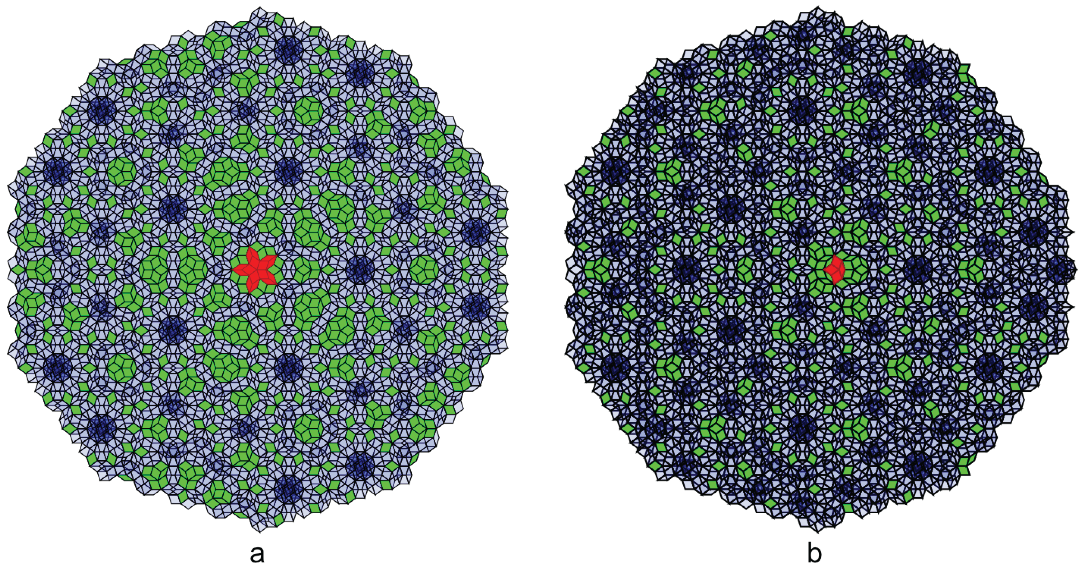
Figure 13a shows all the tiles whose projection in the orthogonal space falls in the possibility-space-window of the given patch (colored red) - the star vertex configuration of the Penrose tiling. These tiles are called the possibility space for the given patch. Notice that in this possibility space, the green tiles are the only possible tiles for that location, while the blue ones superimpose with each other. This implies that the green tiles are forced by the given local patch and therefore belong to the empire of the patch, while the blue tiles are not forced. Also, from the discussion in previous paragraphs, the projection of all the forced green tiles in the orthogonal space falls inside of the empire-window. One can also see that the part of the tiling outside the empire consists completely of the projection of full cubes from the mother lattice and forms a network of strings of these rows of projected cubes. Figure 13b shows the results for a local patch that does not have 5-fold symmetry. One can see that its empire has similar symmetry patterns as the given patch itself.
The key process of the cut-and-project method for calculating empires is to reverse the given patch to its mother lattice and apply the restrictions there. This enables us to calculate the empires for very complicated quasicrystals whose mother lattice is a complex decoration of the simple lattices and even a defected quasicrystal, which is a cut-and-project from a defected mother lattice by a defected cut-window [13].
Figure 14 shows the cut-and-project results for the rest of local vertex types in Penrose tiling. Notice that the empire calculated by the cut-and-project method perfectly matches the result by the multigrid method. Indeed these two methods are mathematically equivalent, although the cut-and-project method has more advantages that will be discussed in the following section.
5. Comparison between the Multigrid Method and the Cut-and-Project Method
In this section, we first prove the mathematical equivalence of the multigrid method and the cut-and-project method in generating the empires in Penrose tiling. Then, in the second part, we give a one dimensional example of the advantage of the cut-and-project method that allows us to calculate the empires in a defected quasicrystal.
5.1. The Parallel between the Multigrid Method and the Cut-and-Project Method
To see the correspondence between the pentagrid and cut-and-project methods for generating Penrose tiling, we begin with , where are the norm vectors of the grids, as used in the pentagrid method. The transpose of is
The matrix represents a linear map where . This is the same transformation used in the pentagrid method to map each mesh to its corresponding dual point .
Notice from Equation (25) that and are the row-vectors of , which are orthogonal in as their dot product is zero. We take to be the normalized vectors and the subspace spanned by the orthonormal basis , with , the orthogonal projection onto E.
The standard basis vectors of project orthogonally down onto E symmetrically, creating a pentagonal star of vectors inscribed on E. All the projected vectors have equal length and in fact, when expressed in terms of the basis , are a direct scaling of the pentagonal star of unit-length vectors , as used in the pentagrid method.
Let denote the grid in , which lies perpendicular to the coordinate vector and which is shifted away from the origin by .
We consider the translation of the plane E by a shift vector , . Each grid intersects in a series of evenly spaced parallel lines, which are perpendicular to the projected vector . Let be the grid inscribed in defined as the intersection . The spacing between grid lines is and each grid line can be expressed in the basis as . The factor provides the dilation necessary to relate the copy of from Section 3 (which contains a pentagrid with unit-length grid vectors and unit-spacing between grid lines), with the copy of parametrized by the basis (which contains a pentagrid with grid vectors with a uniform grid spacing of ).
In other words, if we choose to parametrize with the basis where , then the grid line can be written relative to as . This is precisely the equation used to define the pentagrid in Section 3.
In , the mesh regions located between the grid hyperplanes have the form . This describes the interior of a unit 5-cubes, which is centered around a certain coordinate integer lattice point . This coincides with the Voronoi cells for the lattice . In other words, each mesh is exactly the interior of a certain Voronoi cell centered at a lattice point .
Consider now a mesh , intersecting non-trivially, so that . The boundary of intersects with to form the grid lines inscribed in , which define the boundary of the planar mesh region . The region is expressed as , in terms of the basis for E.
In the multigrid method, a vertex of the form is included in the dual tiling as long as the mesh region corresponding to , , is non-empty, in which case the strips have a non-trivial intersection in the plane . When a planar strip is mapped onto using the basis , the image is equal to the intersection of with the corresponding strip in defined by . If the planar strips intersect in a non-empty planar mesh region , then maps onto as the non-empty mutual intersection of the strips with the plane . In other words, there is a Voronoi cell such that . In this way, the multigrid method and the cut-and-project method produce the same set of lattice points that are to be mapped to to be included as vertices in the dual.
In the multigrid method, the transformation is used to map lattice points to the dual vertices. With the cut-and-project method, the points are mapped onto by orthogonal projection . This projected point is expressed in the basis as . So the mapping is identical (up to a scaling by ) to the mapping .
This shows that the two methods are equivalent mathematically. However, from Figure 13 and Figure 14, we can see the the cut-and-project method is conceptually clearer and easier to understand using the possibility space. Also, due to the fact that in the cut-and-project method there is a one-to-one correspondence between the quasicrystal tiles and the facets in the multidimensional lattice, the cut-and-project method has its unique advantages, that is, it can calculate the empires in a defected quasicrystal. The common defects in the quasicrystal can be translated into defects in the cut-window in the mother lattice, which will not affect the calculation of the empires for the local patches. These kind of defects can be used to guide the quasicrystal growth and the phason dynamics in the quasicrystals. A one dimensional example of calculating the empires in a defected quasicrystal is shown below.
5.2. Empires in a Defected Quasicrystal
The empires for the Fibonacci word addressed in Section 2 can also be obtained using the cut-and-project method applied to the lattice projecting onto a line of slope .
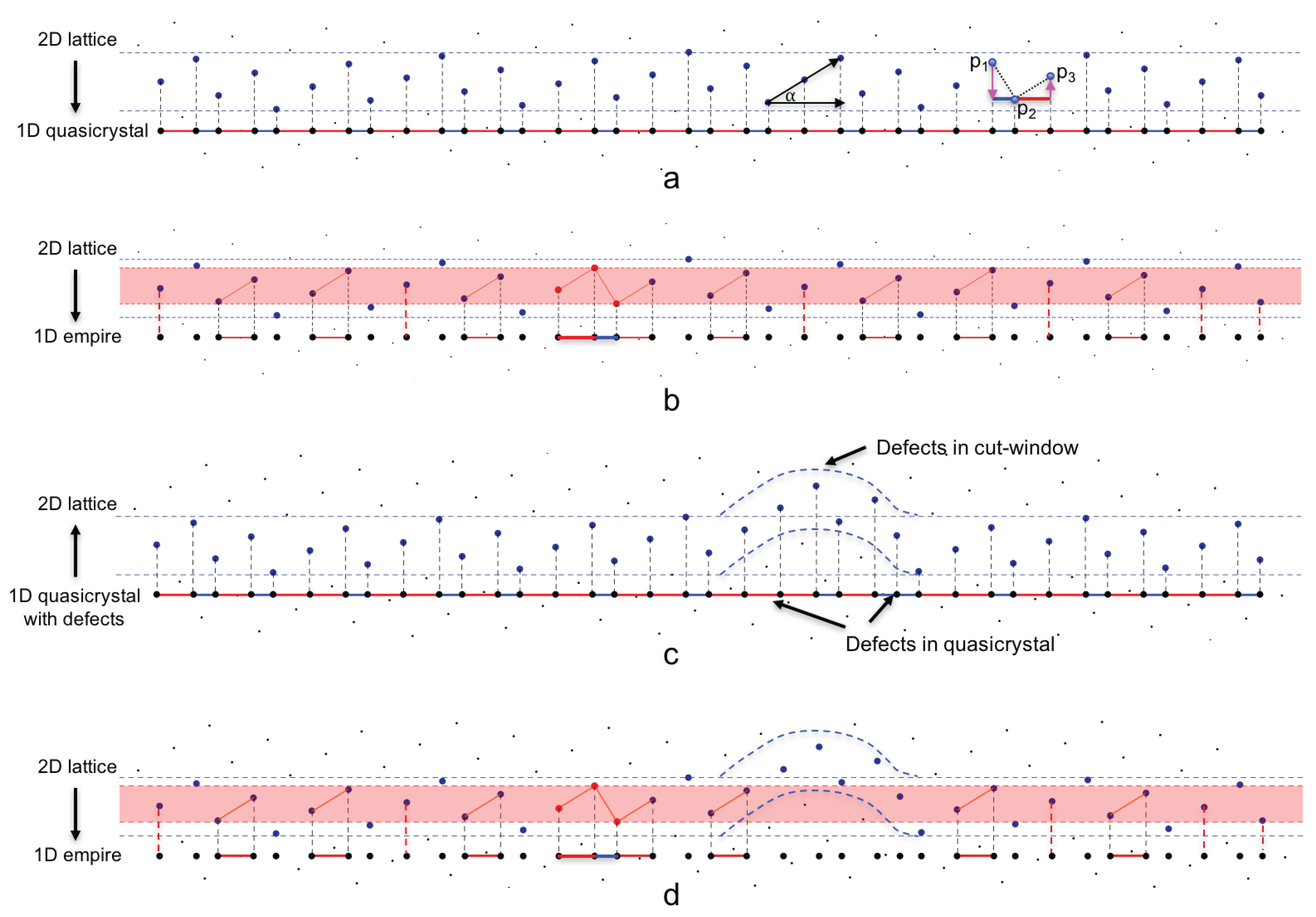
A lattice point whose orthogonal projection onto falls within the cut-window, , is selected to have its projection onto E included in a tiling of E, as shown in Figure 15a. In Figure 15a, the black points are the lattice points, which are rotated by , so that the horizontal axis is aligned with the quasicrystal space E. In this case, E is 1-dimensional so the tiling will consist of points and the edges connecting the neighboring points. If two lattice points are neighbors in , then the unit-length edge connecting them projects onto E as the edge connecting the projected points and . There are two parallel edge classes in these selected edges, one class projects to E to a longer length (colored red in Figure 15a) and the other projects to E to a shorter length (colored blue in Figure 15a), where . The pattern of L’s and S’s along E is the infinite Fibonacci word .
Selecting a sub-word W corresponds to selecting the appropriate edges in , the edges connecting the red points in Figure 15b. The corresponding lattice points (colored red) project onto and their convex hull in gives a new interval as the local-patch-window defined earlier. The intersection of all the valid cut-window, , that cover this , defines the empire-window (colored red in Figure 15b).
The lattice edges whose projection onto falls within the empire-window project onto E as the empire of the selected word W, as the red horizontal segments shown in Figure 15b. Also in the Ammann bar case mentioned in Section 2, all points, not only the segments that have two end points, belong to the empire. That is because we are concerned with all bars (corresponding to points in the quasicrystal), instead of adjacent-bar pairs. In Figure 15b, these extra stand-alone points are from the projection marked by the red dashed lines. These points, each corresponding to a bar, are considered part of the empire in the Ammann bar case.
What if the Fibonacci word is not perfect, or in other words, it has defects in it? Here we introduce a reversing algorithm to bring the one dimensional quasicrystal to its two dimensional mother lattice, with a one-to-one mapping between both the points and the edges. In this case the defect in the one dimensional quasicrystal corresponds to a “defected” cut-window in the lattice. By forcing the cut-window to be perfect, without “defect”, we can still calculate the empire of local patches.
To reverse the Fibonacci words to two dimensions, first we reverse the points in the one dimensional quasicrystal to its corresponding points in , which implies that we keep the one dimensional coordinates of the points to be the x coordinate and add a y coordinate or “height” to the points. The relative height between two adjacent points depends on whether there is an L or S between the points. The pink arrows in Figure 15a show that an S corresponds to a drop of height of , and an L corresponds to a rise of height of . Therefore, knowing the height of one point, the heights of all other points can be determined using this algorithm. Since the height of the points are relative, we can always pick one point and set its height to be zero and from there, the height or y coordinates of all other points can be calculated. Figure 15c shows this reversing procedure. We start with the same Fibonacci word used in Figure 15a, but with some defects added in. First, we reverse all points in this one dimensional quasicrystal to points in two dimensions, using the aforementioned method. After reversing to two dimensions, some of the points at the defected place are off the cut-window used in Figure 15a. It is as though the defects in the one dimensional quasicrystal are translated to the defects in the cut-window in two dimension.
The next step is to calculate the empire of a local patch in this defected quasicrystal by applying the empire-window of the same local patch to these reversed points, based on the fact that the empire of a local patch should only include the valid tiles from the quasicrystal. Comparing Figure 15a,d, we see that the empire-window, colored red, misses three points and one edge, therefore, the empire filters out the defects in the quasicrystal. Thus, this property of the empire can be used for error-corrections in quasicrystal dynamics and growth.
6. Summary and Outlook
A quasicrystal carries non-local information since it is a projection from a higher dimensional crystal. This leads to interesting properties in its growth and dynamics. For example, the quasicrystalline relaxation of a dynamic system and the self-correction in quasicrystal growth. The non-local feature of a quasicrystal is best represented in the empires of this quasicrystal, which can serve as an important guiding principle for crystal growth and dynamics.
In this paper we first reviewed two existing methods, the Fibonacci grid method and the multigrid method, for computing the empires for a local patch in quasicrystals using Penrose tiling as an example and we introduced a new and more efficient method, the cut-and-project method.
The Fibonacci grid method using Ammann bars provides some interesting insights but ultimately is inconvenient in practice. Moreover, it is known that the method sometimes does not capture all the forced Ammann bars and so it may fail to identify all the forced tiles in a given empire. The multigrid method provides a robust algorithm not only for generating Penrose tiling but for computing empires as well. There is a disconnect, however, between the tiling and the pentagrid which was used to create it. Namely, given a set with defected tiles, it is difficult to find an appropriate arrangement of grid lines which provides those tiles somewhere in their dual.
The existing methods for generating the empires in a quasicrystal are not very efficient in simulating a dynamics system, while the new method we discovered, a method that uses the cut-and-project technique, is very efficient computationally and also, it provides an explanation of the relaxation and self-correction of quasicrystals. Our new method, the cut-and-project method, provides the same amount of computational robustness as the pentagrid method, but has the added benefit of providing a direct link between the tiles of the quasicrystal and the corresponding facets of the mother lattice. Also, the fact that it can calculate the empires for defected quasicrystals makes it an important tool for the error-correction in quasicrystal growth and dynamics.
Defects occur during the dynamics or growth of quasicrystals and the empires can self correct them by help perfecting the cut-window. We conjecture that a perfect cut-window, reinforced by the sum of the empires of all the stabilized local patches, corresponds to a relaxed ground energy state. And fluctuation in the energy will cause modulation/defects in the cut-window, therefore resulting in defects in the projected quasicrystal. Relaxing the system indicates perfecting the cut-window which leads to the self-correction in quasicrystal dynamics, especially in quasicrystal growth, where at the center, the quasicrystal is relaxed, therefore with no or fewer defects, while at the edge, the quasicrystal is unstable, therefore with more defects. But as soon as this part is relaxed and stabilized, the defects will be corrected. This conjecture is consistent with the results of [1]. Our group has been working on a Hamiltonian model based on the empires of one dimensional and two dimensional quasicrystals. The work has successfully simulated the relaxation of a one dimensional system and will soon finish simulating a two dimensional system [13].
Acknowledgments
We thank Sinziana Paduroiu for her comments and for her generous help on technical writing and editing. We are grateful to the anonymous referees for their suggestions and comments.
Author Contributions
Fang Fang reviewed the two existing methods for generating empires (the Fibonacci grid method and the multigrid method) and discovered the new method, the cut-and-project method. Dugan Hammock helped reproduce the results using the multigrid method and helped produce the figures in this paper. They both proved independently the similarities between the multigrid method and the cut-and-project method. Klee Irwin is the leader and founder of the research team and he envisioned the application of empires in quasicrystal dynamics and quasicrystal growth.
Conflicts of Interest
The authors declare no conflict of interest.
References
- Nagao, K.; Inuzuka, T.; Nishimoto, K.; Edagawa, K. Experimental observation of quasicrystal growth. Phys. Rev. Lett. 2015, 115, 075501. [Google Scholar] [CrossRef] [PubMed]
- Grunbaum, B.; Shephard, G.C. Tilings and Patterns; W.H. Freeman and Company: New York, NY, USA, 1987. [Google Scholar]
- Conway, J.H. Triangle tessellations of the plane. Am. Math. Mon. 1965, 72, 915. [Google Scholar]
- Effinger-Dean, L. The Empire Problem in Penrose Tilings. Bachelor Thesis, Williams College, Williamstown, MA, USA, 2006. [Google Scholar]
- Penrose, R. The role of aesthetics in pure and applied mathematical research. Bull. Inst. Math. Appl. 1974, 10, 266–271. [Google Scholar]
- Socolar, J.E.S.; Steinhardt, P.J. Quasicrystals. II. Unit-cell configurations. Phys. Rev. B 1986, 34, 617–647. [Google Scholar] [CrossRef]
- Senechal, M.J. Quasicrystals and Geometry; Cambridge University Press: Cambridge, UK, 1995. [Google Scholar]
- Minnick, L. Generalized Forcing in Aperiodic Tilings. Bachelor Thesis, Williams College, Williamstown, MA, USA, 1998. [Google Scholar]
- Fang, F.; Irwin, K. An icosahedral quasicrystal and E8 derived quasicrystals. arXiv, 2015; arXiv:1511.07786. [Google Scholar]
- Gahler, F.; Rhyner, J. Equivalence of the generalized grid and projection methods for the construction of quasiperiodic tilings. J. Phys. A Math. Gen. 1986, 19, 267–277. [Google Scholar] [CrossRef]
- De Bruijn, N.G. Algebraic theory of Penrose’s non-periodic tiling. Proc. Kon. Ned. Akad. Wetensch. 1981, 84, 39–66. [Google Scholar] [CrossRef]
- Henley, C.L. Sphere packing and local environments in Penrose tilings. Phys. Rev. B 1986, 34, 797–816. [Google Scholar] [CrossRef]
- Sen, A.; Aschheim, R.; Fang, F.; Irwin, K. Emergence of aperiodic order in a random tiling network using Monte Carlo simulations. Manuscript in preparation.
Figure 1.
The prolate and oblate rhombuses in Penrose tiling decorated with segment lines.
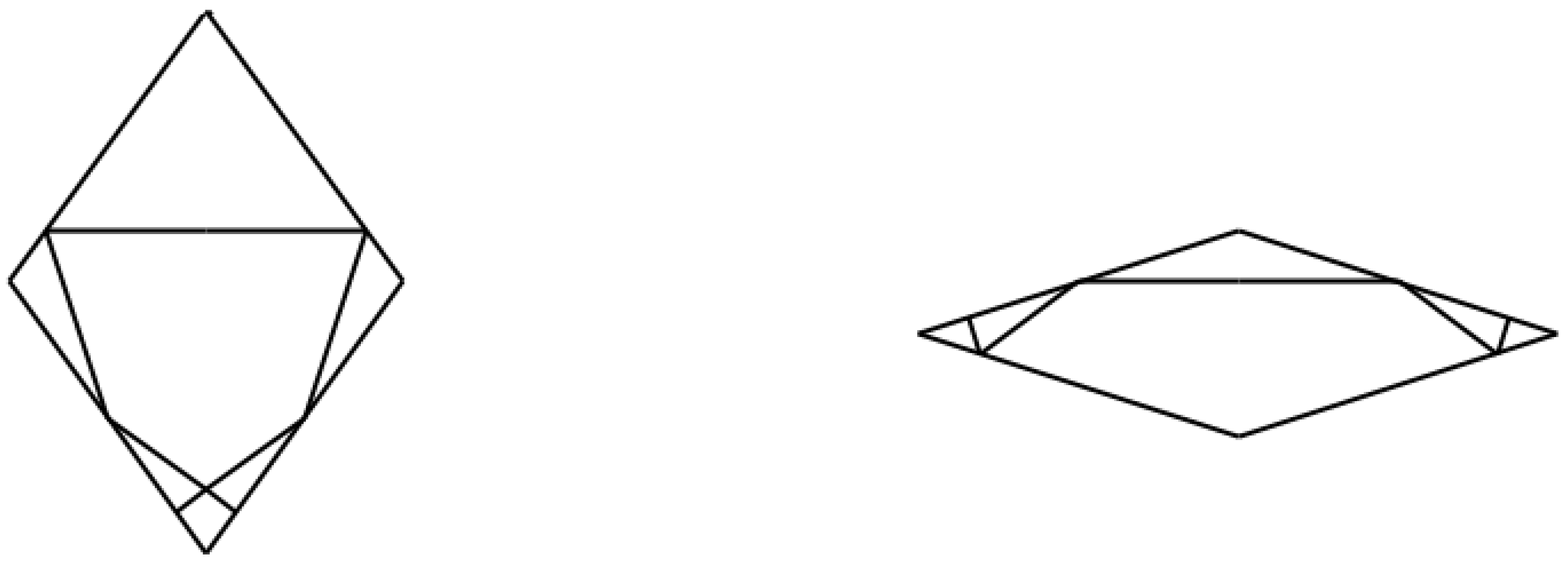
Figure 2.
Ammann bars in Penrose tiling.
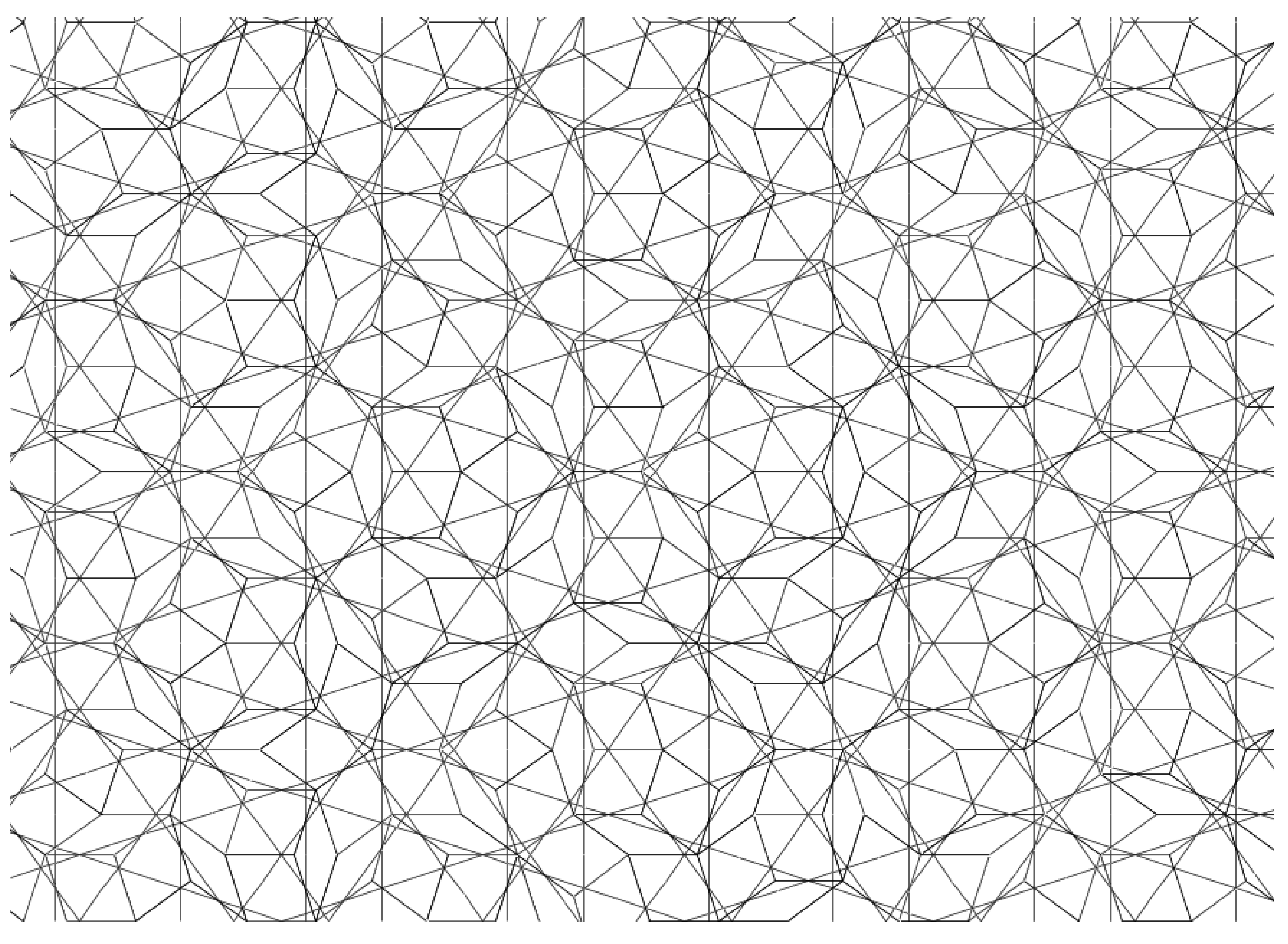
Figure 3.
An example of the resulting empire of the star vertex configuration. The blue bars are the first set of the forced bars and the red ones are the second set. The center patch is the given vertex configuration and the tiles surrounding it are the forced tiles that make up the empire.
Figure 3.
An example of the resulting empire of the star vertex configuration. The blue bars are the first set of the forced bars and the red ones are the second set. The center patch is the given vertex configuration and the tiles surrounding it are the forced tiles that make up the empire.

Figure 4.
An example of a pentagrid where , ,…, are the grid vectors.

Figure 5.
The grid as a set of parallel planes indexed by . is the norm vector and is the shift of the grid.
Figure 5.
The grid as a set of parallel planes indexed by . is the norm vector and is the shift of the grid.

Figure 6.
The dualizing procedure for generating a Penrose tiling from a pentagrid. To construct a Penrose tiling, first we identify the intersections in a sample patch in the pentagrid (a) and then we construct a dual quasicrystal cell, here the prolate and oblate rhombuses, at each intersect point, placing them edge to edge while maintaining their topological connectedness (b).
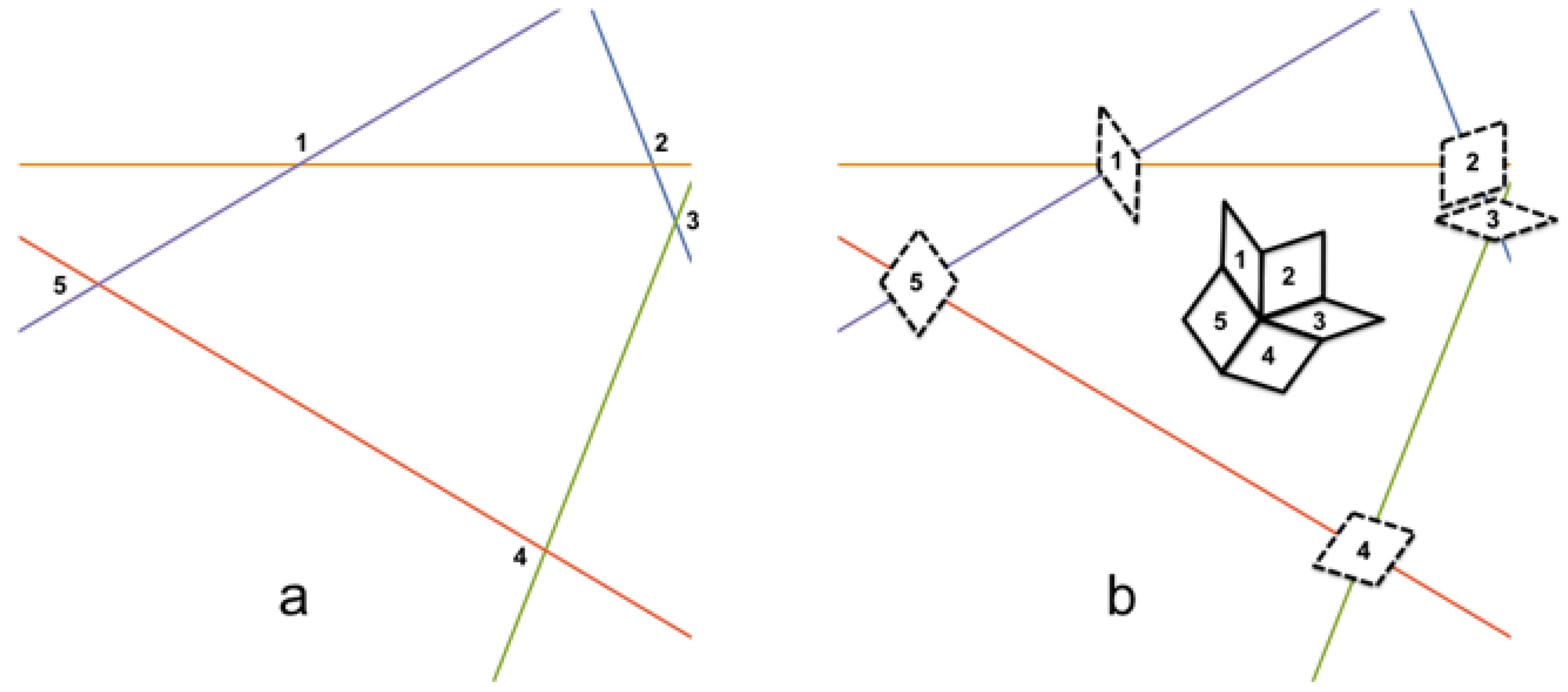
Figure 7.
Calculating the coordinates of the vertices in the Penrose tiling using the indices of the corresponding mesh regions. (a) open strips in grid , where is the norm of the and is the shift vector; (b) a mesh region containing a point x, which is given by the intersection of strips from all five grids; (c) an intersection point in the grid and its corresponding tile in the tiling.

Figure 8.
Results of the empire calculation for two different local vertex types in Penrose tiling, using the multigrid method. The green tiles are the forced tiles (empire) by the local vertex configuration (red), while the blue tiles are not forced.
Figure 8.
Results of the empire calculation for two different local vertex types in Penrose tiling, using the multigrid method. The green tiles are the forced tiles (empire) by the local vertex configuration (red), while the blue tiles are not forced.
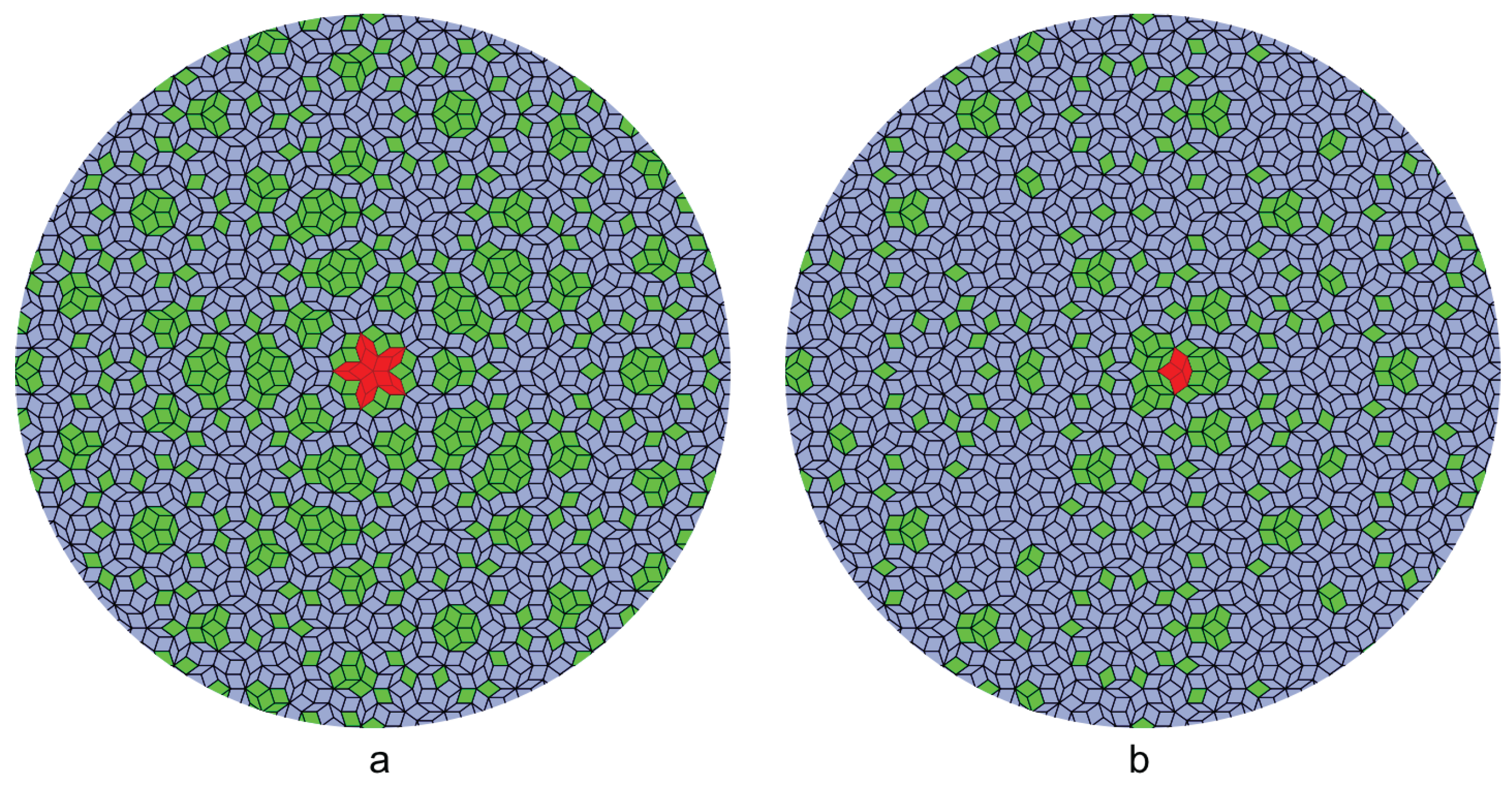
Figure 9.
Results of the empire calculation for the rest of vertex types in Penrose tiling, using the multigrid method. For each vertex type, an enlarged center vertex configuration is shown at the lower right corner of its empire.
Figure 9.
Results of the empire calculation for the rest of vertex types in Penrose tiling, using the multigrid method. For each vertex type, an enlarged center vertex configuration is shown at the lower right corner of its empire.
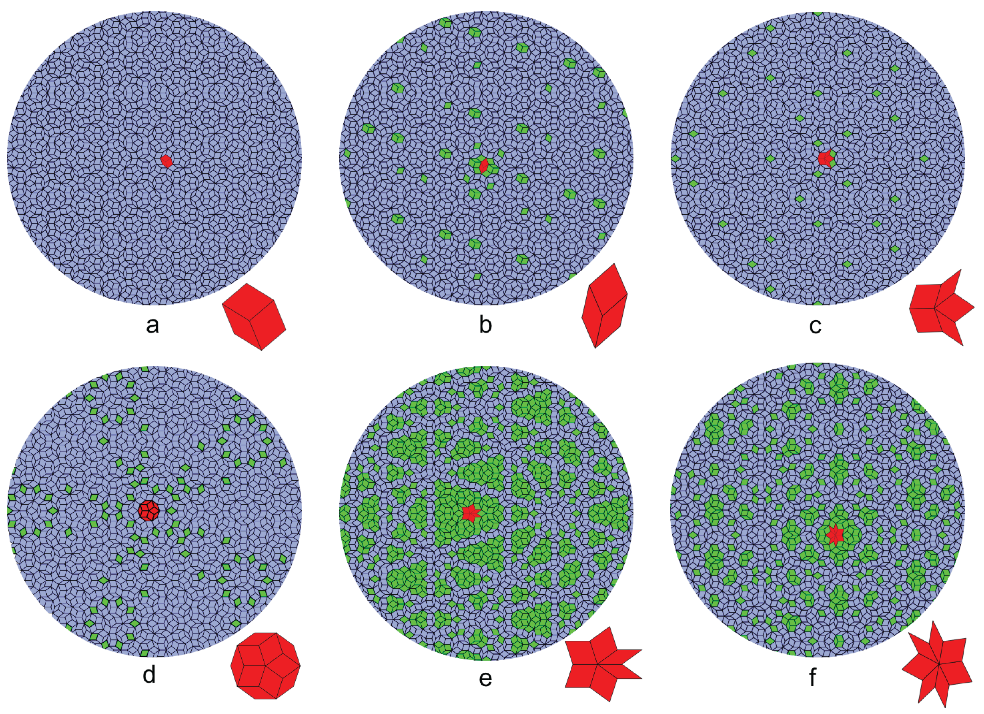
Figure 10.
A schematic diagram showing two ways of interpreting the cut-and-project method for generating a quasicrystal from a higher dimensional lattice. (a) shows that the points are selected for projection as long as there is non-trivial intersection between their Voronoi cell and the quasicrystal space. The black points are the lattice points, and the hexagons are their Voronoi cells, E is the quasicrystal space, is the orthogonal space, and the solid blue and green segments are the projected tiles in the quasicrystal space; (b) shows that the points are selected for projection as long as their projection on the orthogonal space falls inside of .
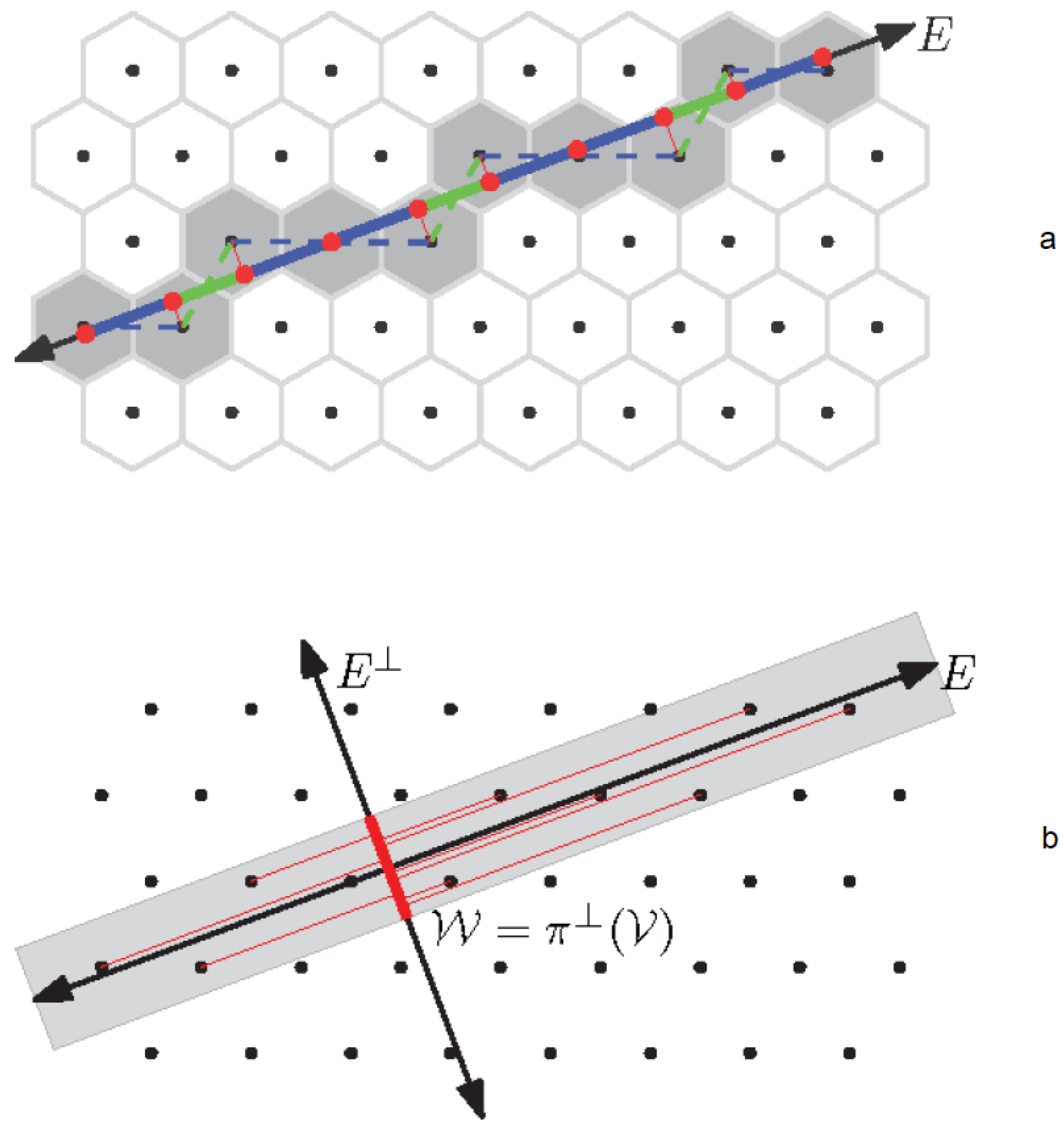
Figure 11.
The cut-window for projecting to 2D Penrose tiling.
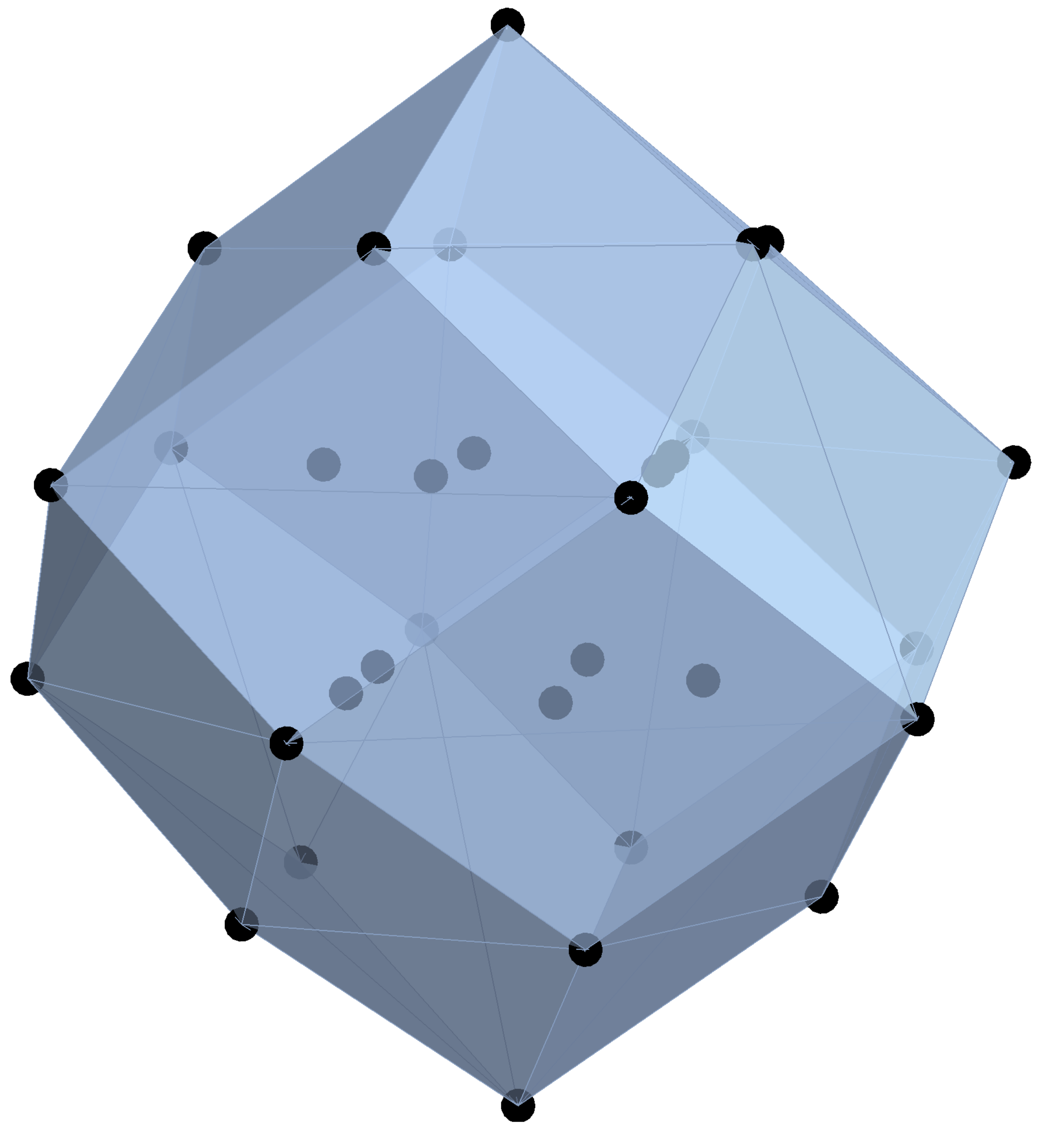
Figure 12.
Illustration of the shifting of the cut-window in the direction of one of its norm vectors.
Figure 12.
Illustration of the shifting of the cut-window in the direction of one of its norm vectors.
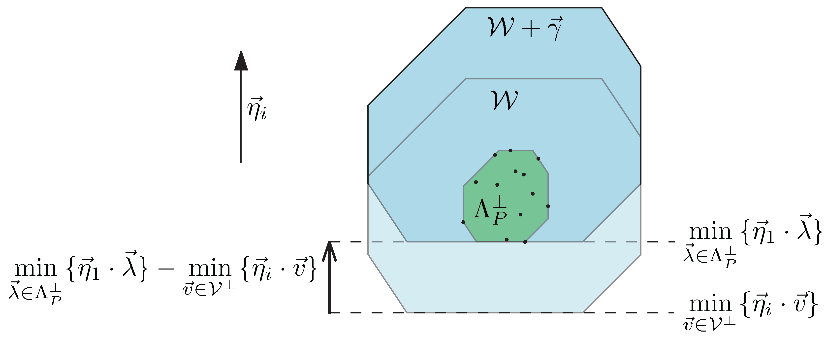
Figure 13.
Results of the empire calculation for two different local vertex types in Penrose tiling, using the cut-and-project method; (a) shows the empire of the vertex type S5 and (b) shows the empire of the vertex type K. The green tiles are the forced tiles (empire) by the local vertex configuration (red), while the gray superimposed tiles are not forced. Notice that the gray tiles are projection of faces of full cubes from Z5 and they form networks of these projected cubic strings.

Figure 14.
Results of the empire calculation of the rest of the vertex types in Penrose tiling, using the cut-and-project method. For each vertex type, an enlarged center vertex configuration is shown at the lower right corner of its empire.
Figure 14.
Results of the empire calculation of the rest of the vertex types in Penrose tiling, using the cut-and-project method. For each vertex type, an enlarged center vertex configuration is shown at the lower right corner of its empire.
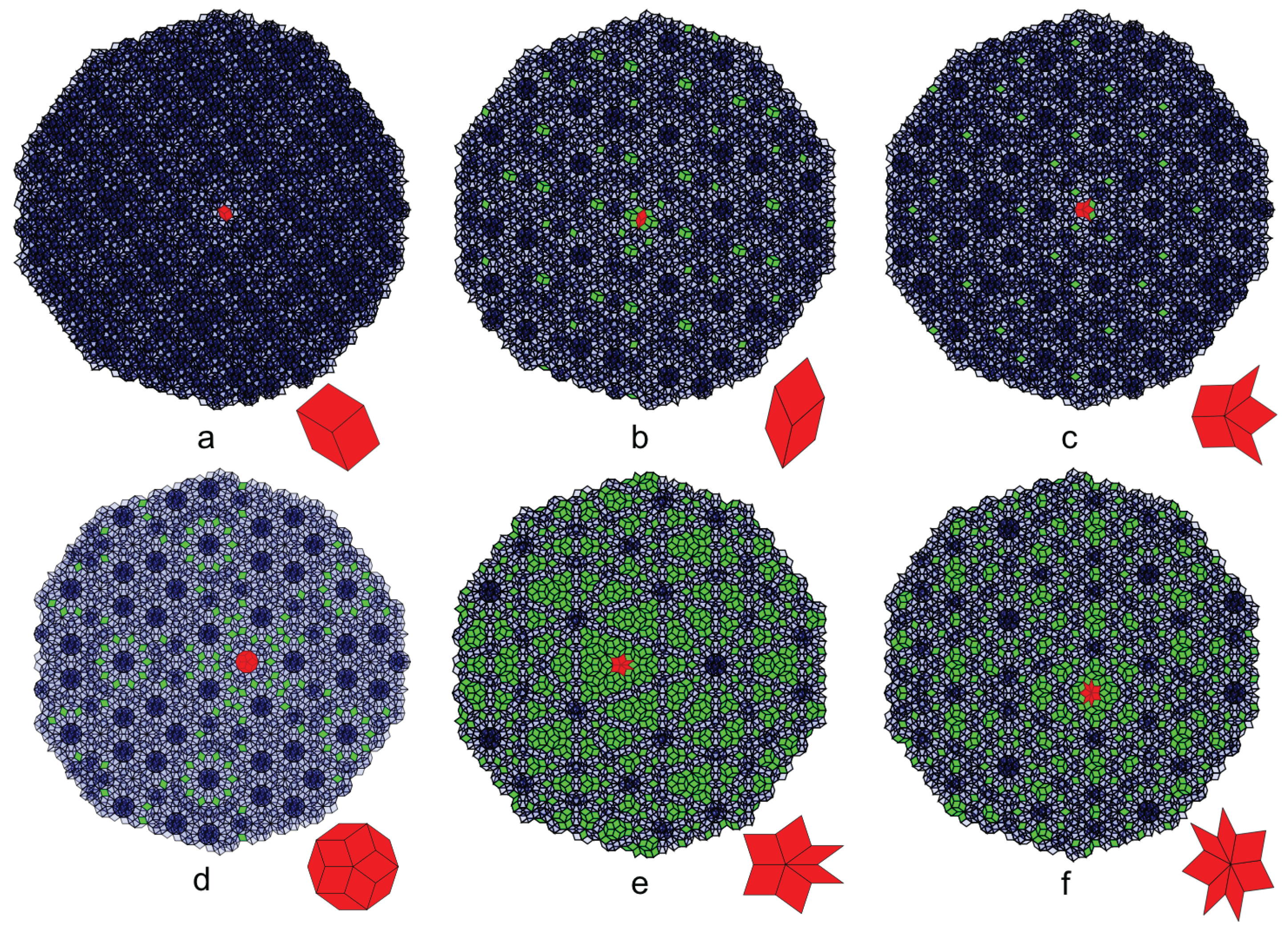
Figure 15.
(a) Illustration of the cut-and-project method for obtaining a one dimensional quasicrystal, the Fibonacci word, from the lattice; (b) illustration of the cut-and-project method for obtaining the empires in the Fibonacci word; (c) illustration of the reversing cut-and-project process, from a defected Fibonacci word to corresponding points in the two dimensional lattice; (d) illustration of the cut-and-project method for obtaining the empires in the defected Fibonacci word.

© 2017 by the authors. Licensee MDPI, Basel, Switzerland. This article is an open access article distributed under the terms and conditions of the Creative Commons Attribution (CC BY) license (http://creativecommons.org/licenses/by/4.0/).
Share and Cite
MDPI and ACS Style
Fang, F.; Hammock, D.; Irwin, K. Methods for Calculating Empires in Quasicrystals. Crystals 2017, 7, 304. https://doi.org/10.3390/cryst7100304
AMA Style
Fang F, Hammock D, Irwin K. Methods for Calculating Empires in Quasicrystals. Crystals. 2017; 7(10):304. https://doi.org/10.3390/cryst7100304
Chicago/Turabian StyleFang, Fang, Dugan Hammock, and Klee Irwin. 2017. "Methods for Calculating Empires in Quasicrystals" Crystals 7, no. 10: 304. https://doi.org/10.3390/cryst7100304
Note that from the first issue of 2016, this journal uses article numbers instead of page numbers. See further details here.