Shifting the Shear Paradigm in the Crystallographic Models of Displacive Transformations in Metals and Alloys

LMTM, EPFL (Ecole Polytechnique Fédérale de Lausanne), Neuchatel 2000, Switzerland
Crystals 2018, 8(4), 181; https://doi.org/10.3390/cryst8040181
Submission received: 2 March 2018
/
Revised: 6 April 2018
/
Accepted: 16 April 2018
/
Published: 23 April 2018
(This article belongs to the Special Issue Microstructures and Properties of Martensitic Materials)
Abstract
:Deformation twinning and martensitic transformations are characterized by the collective displacements of atoms, an orientation relationship, and specific morphologies. The current crystallographic models are based on the 150-year-old concept of shear. Simple shear is a deformation mode at constant volume, relevant for deformation twinning. For martensitic transformations, a generalized version called invariant plane strain is used; it is associated with one or two simple shears in the phenomenological theory of martensitic crystallography. As simple shears would involve unrealistic stresses, dislocation/disconnection-mediated versions of the usual models have been developed over the last decades. However, a fundamental question remains unsolved: how do the atoms move? The aim of this paper is to return to a crystallographic approach introduced a few years ago; the approach is based on a hard-sphere assumption and linear algebra. The atomic trajectories, lattice distortion, and shuffling (if required) are expressed as analytical functions of a unique angular parameter; the habit planes are calculated with the simple “untilted plane” criterion; non-Schmid behaviors associated with some twinning modes are also predicted. Examples of steel and magnesium alloys are taken from recent publications. The possibilities offered in mechanics and thermodynamics are briefly discussed.

1. The Origin of the Concept of Simple Shear
Mechanical twinning and martensitic transformations are known to form very rapidly, sometimes at the velocities close to the speed of sound; the atoms move collectively, and the product phase (martensite or twins) appear as plates, laths, or lenticles. These transformations are called “displacive” in metallurgy (please note that the meaning of this term is different from the one used in physics, where “displacive” implies only small displacements of atoms without breaking the atomic bonds). In his extensive review, Cahn [1] wrote: “Cooperative atom movements in phase transformations may extend over quite large volumes of crystals. When this happens, the transformation is termed martensitic (from Martens, who discovered the first transformation of this type in carbon steel). If the atom movements in a crystal results in a new crystal of different orientation, but identical structure, the process is termed mechanical twinning.” Christian and Mahajan [2] also insisted on the great similarities between deformation twinning and martensite transformations: “all deformation twinning should strictly be regarded as a special case type of stress-induced martensitic transformation”.
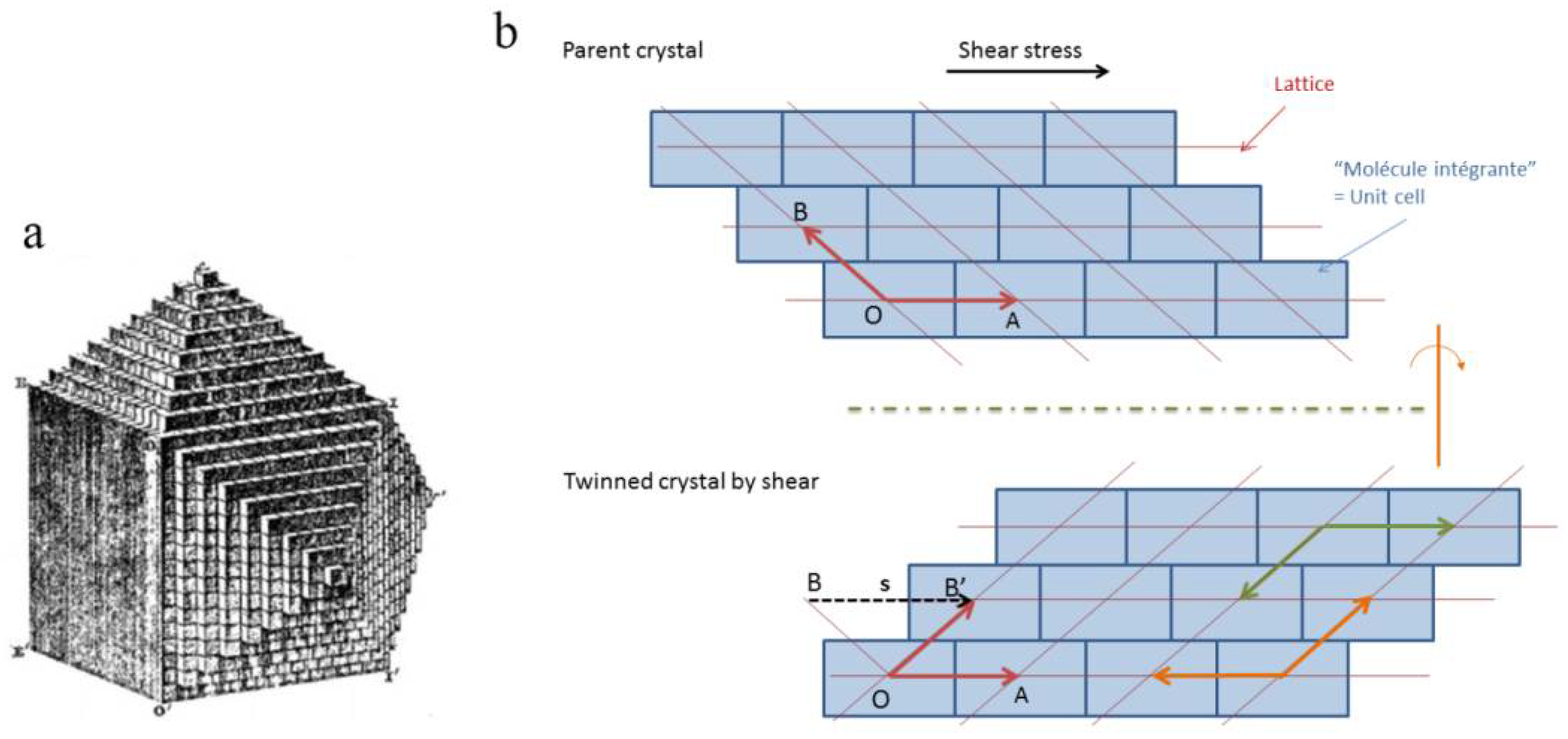
Simple shears are the cornerstone of the theories of deformation twinning and martensitic transformation developed during the last century [1,2,3]. The notion of simple shear can even be traced back to older times, as recalled by Hardouin Duparc [4]. One hundred and fifty years ago, in 1867, William Thomson and Peter Guthrie Tait’s “Treatise on Natural Philosophy” [5] (from [4]) defined that “‘a simple shear’ is the property that two kinds of planes (two different sets of parallel planes) remain unaltered, each in itself”. The mathematical formalism, with the nomenclature K1, η1, K2, and η2, was introduced by Otto Mügge in 1889 [6] (from [4]). At that time, crystallographers and mineralogists already knew the periodic structure of minerals, thanks to Haüy’s works at the beginning of the 19th century [7]. The crystal periodicity was expressed by the lattice, but the concept of the unit cell was yet not fully clarified; it was just a “molecule intégrante”, like a “brick”. Therefore, it was natural at that time to consider that the “bricks” could glide on themselves in order to rearrange and form a new twinned lattice, as illustrated in Figure 1.
At the early beginning of the 20th century, these notions, originally from mineralogists, were acquired by the metallurgists, without any possibility at that time to further clarify the nature of the “bricks”. Remember that atoms were still a speculative idea. Democritus and ancient Greek philosophers supposed their existence, but the first evidence was given in the early 1800s by the chemist John Dalton, who noticed that the chemical reactions always imply ratios of elements in small integers. Dalton also imagined the atoms as solid spheres. The idea of discontinuous matter, however, was not unanimously admitted. In 1827, botanist Robert Brown observed the erratic movements of dust grains floating at the water surface, and the Bownian motion was explained in 1905 by Albert Einstein using statistical physics. The mass and dimensions of the atoms were soon experimentally determined by the physicist Jean Perrin. A new area then opened to specify the properties of the atoms. Very quickly, it appeared with the discoveries of the electron by Thomson and protons by Rutherford, along with quantum physics born with Bohr, that atoms were far more complex than Dalton’s solid spheres. However, in many metals, the hard-sphere assumption holds quite satisfactorily, at least to describe the atomic packings. William Barlow in 1883 [8] noticed that the symmetries of some metals and alloys can be represented by packings of hard spheres, with the body-centered cubic (bcc), the face-centered cubic (fcc), and the hexagonal close-packed (hcp) structures among them. The ratio of lattice parameters c/a in magnesium, cobalt, zirconium, titanium, rhenium, or scandium differs from the ideal packing ratio by less than 3%. The precise determination of the lattice parameters, thanks to X-ray or electron diffraction, revealed that in many bimetallic solid solutions, the lattice parameter of the mixture of two elements is the average of the lattice parameter of each pure element, in agreement with a hard-sphere packing model. During fcc-bcc martensitic phase transitions, the difference of lattice parameters expected by a hard-sphere model is only 4%. The critical shear required to activate dislocations was studied in 1947 by Bragg and Nye [9] with sub-millimeter bubble rafts, and the hard sphere model is still used nowadays in classrooms to explain the ABCABC and ABABAB packings of the fcc and hcp phases, respectively. The hard-sphere model is also an important approximation made in molecular dynamics. However, atoms, even with their simple hard-sphere image, are not explicitly present in the crystallographic theories of twinning and martensitic transformations, which are all based on the lattices and their transformation by shears, as in Mügge’s initial model. The atoms are the “big losers” of these theories.
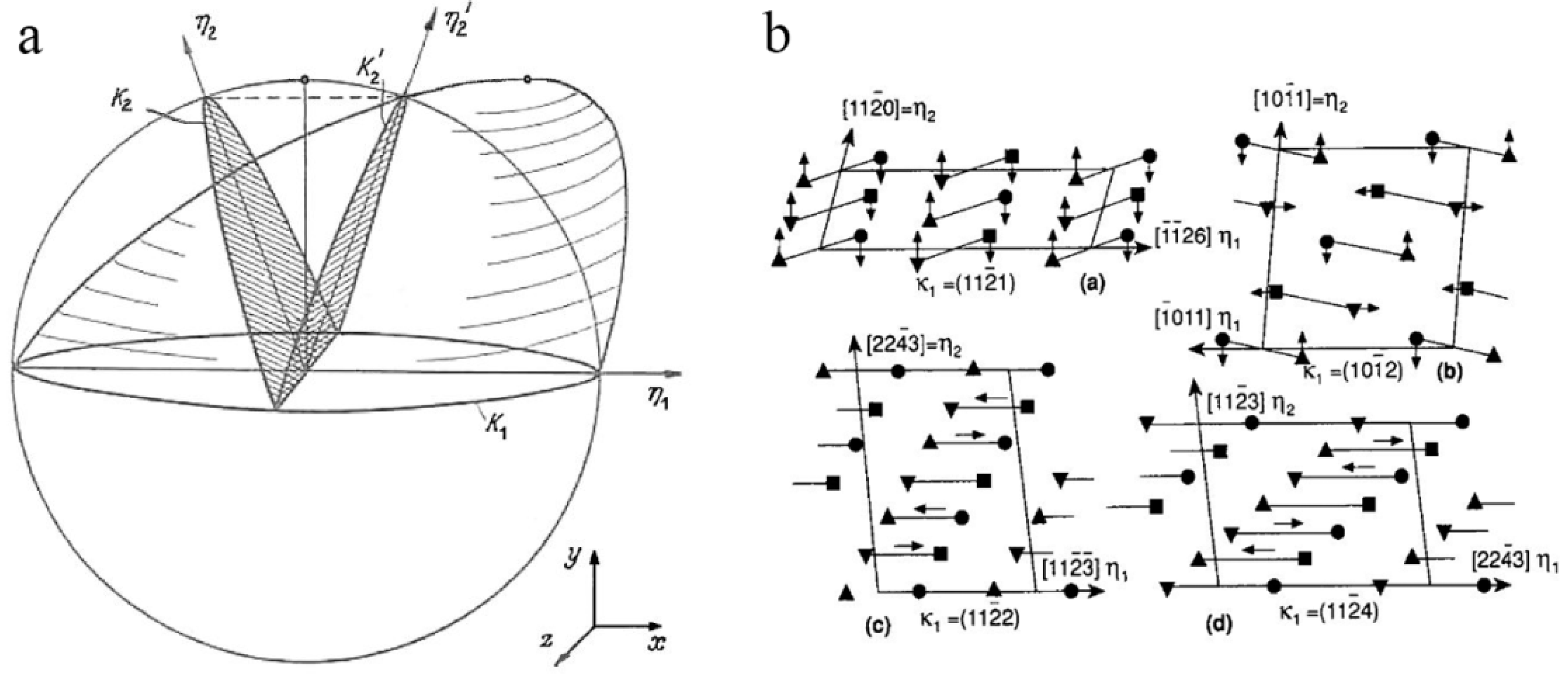
2. Shears Used in the Theories of Deformation Twinning
Cahn wrote about deformation twinning: “That part of the parent crystal which is thus transformed undergoes a macroscopic change of shape which can be described exactly as a simple shear” [1]. A shear is defined by its shear plane K1, its shear direction η1, and its amplitude s1. The shear leaves a second plane (K2) undistorted (but rotated). The direction η2 belongs to K2, and is perpendicular to the intersection between K1 and K2. The plane K2 is rotated by an angle φ, and the shear amplitude is given by s1 = 2 tan(φ/2). It is classic to define two types of twins: type I, where the plane K1 and the direction η2 are rational; and type II, where the plane K2 and the direction η1 are rational. One of these components is a symmetry element that is common to both parent and twin crystal; K1 is a common mirror plane for type I twins, and η1 is a common two-fold axis for type II twins. For any mode I twin, defined by K1 along η1, one can associate a conjugate mode II twin, defined by substituting K2 in place of K1 and η2 in place of η2 [6]. The four components K1, K2, η1, and η2, as well as their geometric representation with the shearing ellipsoid, as represented by Hall in 1954 [10] (Figure 2a) and still used in classical textbooks, date from Thomson and Guthrie Tait, who clearly noted that “the planes of no distortion in a simple shear are clearly the [two] circular sections of the strain ellipsoid” [5] (from Ref. [4]). In the 1950s, the twinning theory was mathematically developed and refined, mainly by Kihô in 1954 [11], Jaswon and Dove in 1956 [12], and later by Bilby et al. [13,14,15], following some of the notions and crystallographic tools used by Bowles and Makenzie in the phenomenological theory of martensite transformation (PTMC), which will be detailed in the next section. The master equation of the crystallographic theory of twinning built by Bilby et al. can be summarized by C = R.S, where C is the correspondence matrix, R is a rotation, and S is a simple shear. These three matrices have a determinant equal to ±1. The correspondence matrix gives the coordinates in the twin basis of the parent basis vectors, once distorted by the shear. As these vectors should be vectors of the twin lattice, the coordinate should be integers, or rational if the cell of the Bravais lattice contains more than one atom (as it is the case for hcp metals) or if a supercell is chosen for the calculations. For these cases, the atoms inside the cell that are not positioned at the nodes of the cell do not follow the same shear trajectory as those positioned at the nodes; one says that they “shuffle” (we will come later on this term). An additional mathematical restriction comes from the fact that the rotation matrix should check R.RT = I, with I being the identity matrix, which permits the establishment of a list of correspondence matrices. Among the numerous (but finite) possible correspondence and shear matrices given by the shear-based twinning theory, only those with the lowest shear amplitude and minimum shuffles are considered to be realistic. For example, fifteen deformation twinning modes could be listed in titanium [15], some of which are reproduced in Figure 2b. The theory is still used today (see for example [16]). Despite the theory’s mathematical sophistication and rigor, one must admit that its fundaments do not differ from the initial 150-year-old view. Despite the progress, the theory does not answer the simple question: how do atoms move during twinning? In the case of a cell made of one atom, it is assumed that the atoms follow the same shear as the nodes of the lattice, but for multiple-atom (super)cells, the shuffling of the atoms is not satisfactorily treated. Some possible modes were proposed by Bilby and Crocker [13]; they often consist in finding the different ways of translating the positions obtained by the shear, in order to reach those obtained by the reflections or the 180° rotation symmetries. The shuffles in these models are very complex, as shown by the arrows of Figure 2b. Shuffling was not examined anymore in the last version of the theory proposed by Bevis and Crocker [14].
Actually, even if not always acknowledged, it seems unrealistic that the atoms can simply move along straight lines, such as drawn by the arrows of Figure 2b; even in the case of one atom per cell. Indeed, for steric reasons the atoms cannot follow simple translations dictated by a simple shear. For a long time, the theories were focused on the way the lattices are deformed, omitting to confront to the question of the atomic trajectories. Therefore, the crystallographic theory of twinning is a phenomenological theory. Assuming that twinning results from a simple shear implies that Schmid’s law [17] should be verified. Deformation twinning should occur when the shear stress resolved along the slip direction on the slip plane reaches a critical value, called the critical resolved shear stress. However, this law is difficult to confirm experimentally (see, for example, “Orientation dependence: is there a CRSS for twinning?” Section 5.1 of [2]). In addition, it was experimentally noticed that some twinning modes in magnesium have “abnormal”, i.e., “non-Schmid” behavior [18]. The reason was attributed to the fact that the local stresses differ from the global ones [19], but to our knowledge, there are no convincing quantitative experimental results that can confirm this explanation. Non-Schmid behavior was also observed at least for slip deformation in bcc metals. In 1928, Taylor wrote “in β-brass resistance to slipping in one direction on a given plane of slip is not the same as resistance offered to slipping in the opposite direction” [20]. This effect, called the twinning-antitwinning effect, was attributed to the core structure of the dislocations in the bcc metals [21,22], but the fundamental reason for the dissymmetry is that Schmid’s law is a continuum mechanics law that does not take into account the atomic structure of the metals, or more precisely, the configuration of the atoms in the stacking of the glide planes or twinning planes. The normal to the {112} bcc twinning plane is not a two-fold rotation axis, which means that a shear along a <111> direction is not equal to a shear in its opposite direction. The same situation exists for deformation twinning in fcc metals: as the direction normal to the {111} plane is a three-fold axis, not a two-fold axis, the shears in the <110> directions are not equal to their opposites. The use of simple or pure shear (both are deformation at constant volume) was proved to be highly efficient in continuum mechanics for describing the plastic behavior of materials, but its direct application to describe the lattice transformation of crystals (packing of discontinuous atoms) raises some important questions that should not be discarded.
3. Shears Used in the Theories of Martensitic Transformations
3.1. Early Models of Martensitic Transformations
For martensitic transformations, the notion of shear was also so pregnant that one could read, “shear transformations are synonymous with martensitic transformations” [23]. However, the first crystallographic model of fcc-bcc distortion proposed by Bain in 1924 [24] does not imply shear. This discrepancy was used to discard Bain’s proposal in the first models of martensitic transformation. Indeed, a few years after Bain’s proposal, the orientation relationship (OR) between the parent fcc and the bcc martensite was experimentally determined, using X-ray diffraction, by Young in 1926 [25], Kurdjumov and Sachs in 1930 [26], Wassermann in 1933 [27], and Nishiyama in 1934 [28]. Young worked on Fe–Ni meteorites, Kurdjumov and Sachs on Fe–1.4C steel, and Nishiyama on a Fe–30Ni alloy. The OR discovered by Young was very close to that discovered by Kurdjumov and Sachs, but history of metallurgy only kept the names of the two latter researchers. The now-called KS OR (for Kurdjumov-Sachs) and NW OR (for Nishiyama-Wassermann) are at 5° from each other, and at 10° from the OR expected by a direct Bain distortion. The difference is non-negligible, which is why Kurdjumov, Sachs, and Nishiyama proposed, in their respective papers, a model of fcc-bcc transformation that is “does not agree” with Bain. Kurdjumov and Sachs imagined a transformation made by two consecutive shears: followed by . Nishiyama proposed a slightly different sequence, in which the first shear is followed by a stretch. These models are quite close and summarized by Nishiyama in his 1934 paper [28] in Figure 3. Therefore, in those models, the fcc-bcc transformation is not a Bain distortion, but neither is it a simple shear—it is a combination of shears or shears and stretch.
The important point of the KSN model is the distortion of the dense plane {111}γ into a dense plane {110}α. Such planar distortion was also noticed and largely discussed by Young, who wrote “On account of the marked resemblance of the (111) plane of the solid solution [taenite, fcc] and the (110) plane in kamacite [bcc], it is possible to form the solid solution by simply shearing rows of atoms and rearranging the atoms in adjacent planes, as already described, a crystal of kamacite which is only a few planes in thickness but of considerable area” [25].
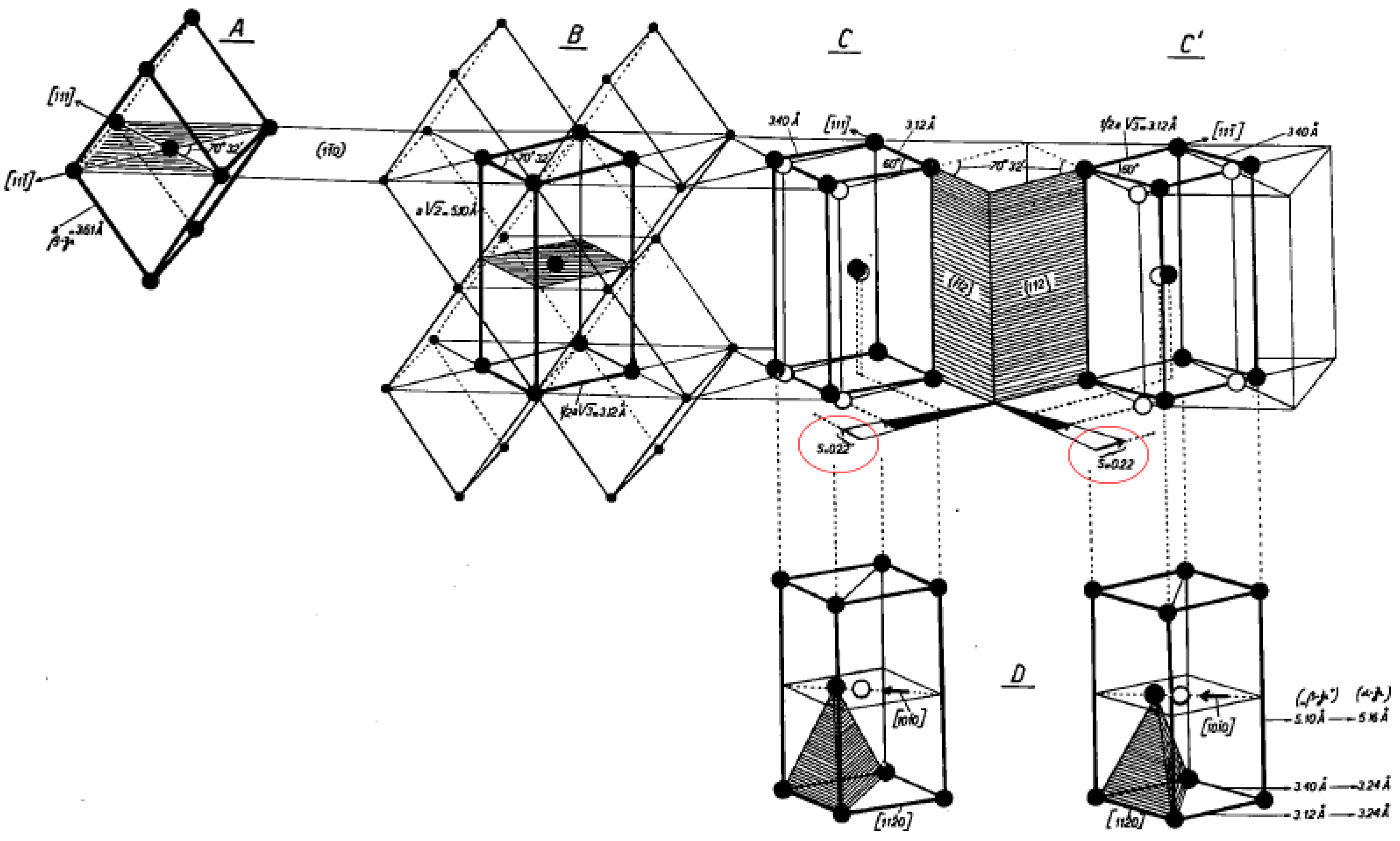
In 1934, Burgers determined the OR in zirconium, between the high temperature parent bcc phase and the low-temperature martensite hcp phase, by X-ray diffraction [29]; as Young, Kurdjumov, Sachs, and Nishimaya did for fcc-bcc transformations, Burgers proposed a crystallographic model of the bcc-hcp transformation. Actually, he treated three models, with one of them implying an intermediate fcc phase—but only the first is now widely accepted. This model is reproduced in Figure 4. Burgers explains it as the combination of “a shear parallel to a {112} plane in the [111] direction lying in this plane, followed by a definite displacement of alternate atomic layers [shuffle] and a homogeneous contraction (eventual dilatation) parallel to definite crystallographic directions.” [29] Burgers also calculated the associated shear value and found s = 0.22. His description is not exactly that of his figure, as two shears are actually applied on two different {112} planes. In order to overcome this problem, it is now usual to replace the shears by a diagonal distortion of the orthorhombic cell, marked by the bold lines in part B of Figure 4, as described (for example) in Kelly and Groves’ book [30]. This distortion is analogous to the Bain distortion in the fcc-bcc transformation, but the difference is that a shuffle is required to put half of the atoms in their good positions and obtain the hcp phase, as shown in the part noted by the letter D in Figure 4.
3.2. The Phenomenological Theory of Martensite Crystallography (PTMC)
The KSN model of the martensitic fcc-bcc transformation was criticized by Greninger and Troaino in their 1949 paper [31], because the KSN model could not explain the observed habit planes in Fe–22Ni–0.8C, and because of the “relatively large movements and readjustments” needed to exactly obtain the fcc structure. They proposed that the “martensite crystal is formed from austenite crystal almost entirely by means of two homogeneous shears” [31]. The details were then clarified by PTMC. One would now say that the first shear explains the shape, i.e., the habit plane of martensite, which is the invariant plane strain (IPS), while the second shear deforms the lattice without changing the shape, because of an “invisible” compensating lattice invariant shear (LIS). The idea of composing two homogeneous shears to obtain an inhomogeneous structure with an invariant plane was then soon associated with the notion of the correspondence matrix, previously introduced by Jaswon and Wheeler in 1948 [32]. This matrix establishes a correspondence between the directions of the fcc and bcc lattices after a Bain distortion. The result forms a mathematical and unified theory that “predicts” both the habit planes and the orientation relationships. This theory was proposed by Weschler et al. [33] and by Bowles and Mackenzie [34,35] in 1953–54. This theory, now called the “phenomenological theory of martensite crystallography” (PTMC), has been adopted by most of the metallurgists, thanks to exhaustive review papers and books, such as those written by Christian [36] and Nishiyama [37], and thanks to the very didactic books written by Bhadeshia [38,39]. The theory of deformation twinning (see previous section) reintroduces most of the mathematical tools used in the PTMC. For the classic fcc-bcc martensitic transformations in steels, the master equation for the PTMC is RB = P1P2, where RB is the product of the lattice deformation comprised of the symmetric Bain stretch matrix B by an additional rotation matrix R, P1 is an IPS, and P2 is a simple shear. PTMC assumes that the simple shear P2 is exactly compensated for by an LIS (P2)−1 produced by twinning or dislocation gliding, such that the martensite shape is only given by P1. The IPS P1 appears as a generalized notion of simple shear that takes into account the volume change of the phase transformation, i.e., the dilatation or contraction component in the direction normal to the shear plane. The IPS gives the shape of the martensite product (lath, plate, or lenticle); the shear plane of P1 is the habit (interface) plane. Both parts of the equations, RB and P1P2, are invariant line strains (ILS), and R is the rotation added to render unrotated the line undistorted by the Bain stretch B. This is usually geometrically illustrated in traditional textbooks, by showing how a sphere is deformed into an ellipsoid and by finding the intersection points between the sphere and the ellipsoid. A summarizing scheme of the IPS and strain matrices used in the PTMC is given in Figure 5b, according to [39].
The PTMC solves the initial issue between the non-shear Bain strain and the specific plate/lath morphologies of martensite that are believed to be the results of shears. The theory is very subtle, and its main inventors introduced important modern concepts in crystallography, such as the coordinate transformation matrix, the transformations from direct to reciprocal spaces, clear references to the bases used for the calculations, correspondence matrices, equations that link the shear matrices with the correspondence and coordinate transformation matrices, etc. It is true that PTMC predicted the existence of twins inside the bcc or body centered tetragonal (bct) martensite formed in steels, and that these twins were not visible by optical microscopy. Their discovery by Nishiyama and Shimizu in the early era of transmission electron microscopy (TEM) in 1956 [40] probably made Nishiyama give up his two-step shear-stretch model (Figure 3) to fully adopt the PTMC. That was not a complete change of mind, according to Shimizu [41]: “he [Nishiyama] foresightedly expected the existence of lattice invariant deformation in martensite a few years before the phenomenological crystallographic theory of martensitic transformation was proposed”. It is plausible that Nishiyama’s rallying to PTMC had a huge impact on the rest of the scientific community, and finally convinced the most recalcitrant metallurgists of that time about the importance of this theory. However, the predictive character of PTMC is often oversold. Some researchers claim that PTMC “predicts all” the martensite features, but this affirmation should be considered thoughtfully. For example, one can be impressed by the apparent prediction of the ORs, but it should be remembered that the PTMC starts from the Bain OR, which is at 10° from the experimentally observed KS or NW ORs, and then it imposes the existence of an invariant line, which makes it closer to KS. If one considers the strong internal misorientations (up to 10°) inside the martensitic products, “finding” an OR close to one belonging to the continuous list of experimentally observed ORs should not be considered as a “prediction”. One should also have a cautious look at the habit planes. The {259} habit planes were explained in 1951 by Machlin and Cohen [42], following Greninger and Troiano’s initial idea of composing shears. The {225} habit planes were explained by Bowles and Mackenzie [34] with a IPS followed by a shear, but with the help of a dilation parameter that was later subject of controversies. The PTMC did not predict these planes, because these planes were already observed before the establishment of the theory; PTMC “only” tried to explain them. The theory did not make predictions but postdictions, which is completely different when the reliability of a theory is considered. Numerous papers were published on the {225} martensite, trying to suppress the dilatation parameter by increasing the level complexity with extra shears (see for examples [43,44]). This “saga” of the {225} habit planes was summarized in 1990 by Wayman [45], and more recently by Dunne [46] as well as Zhang and Kelly [47]. Surprisingly, the fact that the {225} habit planes could be explained by using different methods and different parameters did not raise questions about the real relevance of the PTMC approach. We note here that most of these PTMC studies ignore Jaswon and Wheeler’s paper [32] for the explanation of the {225} habit planes; sometimes they refer to it, but only in the introduction for the use of Bain correspondence. It is worth recalling that Jaswon and Wheeler’s model was discarded by Bowles and Barrett in 1952 [48], because “Jaswon and Wheeler’s picture of the transformation as a simple homogeneous distortion of the lattice is not consistent with the observed relief effects”. We will come back later on this “rejection”, which we considered as an unfortunate missed opportunity. Apart from the {225}, the {557} habit planes have also been the object of much research for more than 60 years, without consensus; most of the studies include additional shears (see for example [49,50]). The last development of the PTMC has mainly consisted in adding or varying the shears and their combinations, i.e., by adding complexity, without being more effective than the initial Bowles-Mackenzie and Weschler-Liebermann-Read models. The “predictions” are sometimes written with six- or eight-digit numbers and compared with experimental results, where accuracy rarely exceeds one digit.
The PTMC has been applied to other transformations, such as bcc-orthorhombic and bcc-hcp transformations [51], and here again the same criticisms can be raised. The theory does not predict orientation relationships, because it starts from Bain-type distortions, which already agree with experimental orientations. In the case of the bcc-hcp transformation, for example, PTMC starts with the ortho-hexagonal cell that was already defined by the Burger’s OR, shown in Figure 4. The habit planes are not predicted, but “explained”, by choosing the LIS twinning systems among those reported by experimental observations, and by adjusting the dilatation parameter and the twinning amplitude in order to fit the calculated habit planes with those experimentally reported, as in [52]. The success of the PTMC for shape memory alloys, in which the transformation strains are lower than in steels, is probably more convincing. However, as admitted by its creators and by most of its promoters, the PTMC is and remains phenomenological. For example, Bhadeshia [38] clearly wrote that “the theory is phenomenological and is concerned only with the initial and final states. It follows that nothing can be deduced about the actual paths taken by the atoms during transformation: only a description of the correspondence in position between the atoms in the two structures can be obtained.” Therefore, it is the same problem as for deformation twinning; the theory does not answer the simple question: how do the atoms move during the transformation?
3.3. Bogers and Burgers’ Model
In 1964, Bogers and Burgers developed a hard-sphere model to respond to this essential question for the fcc-bcc martensitic transformations [53], as illustrated in Figure 6. They noticed that if a shear on a (111)γ plane is applied to a fcc crystal and stopped midway between the initial fcc structure and its twin, the operation distorts the two adjacent {111}γ planes into {110}α planes, as is the case for a Bain distortion. This idea was actually not new, as Cottrell in his book [54] reported that Zener [55] thought that “The face-centred cubic metals, for example, pass through twinning and body-centered cubic configurations when sheared on their slip planes”. However, Bogers and Burgers noticed that actually, the midway structure is not exactly bcc, and another shear on another (111)γ plane is required to obtain the final and correct bcc structure.
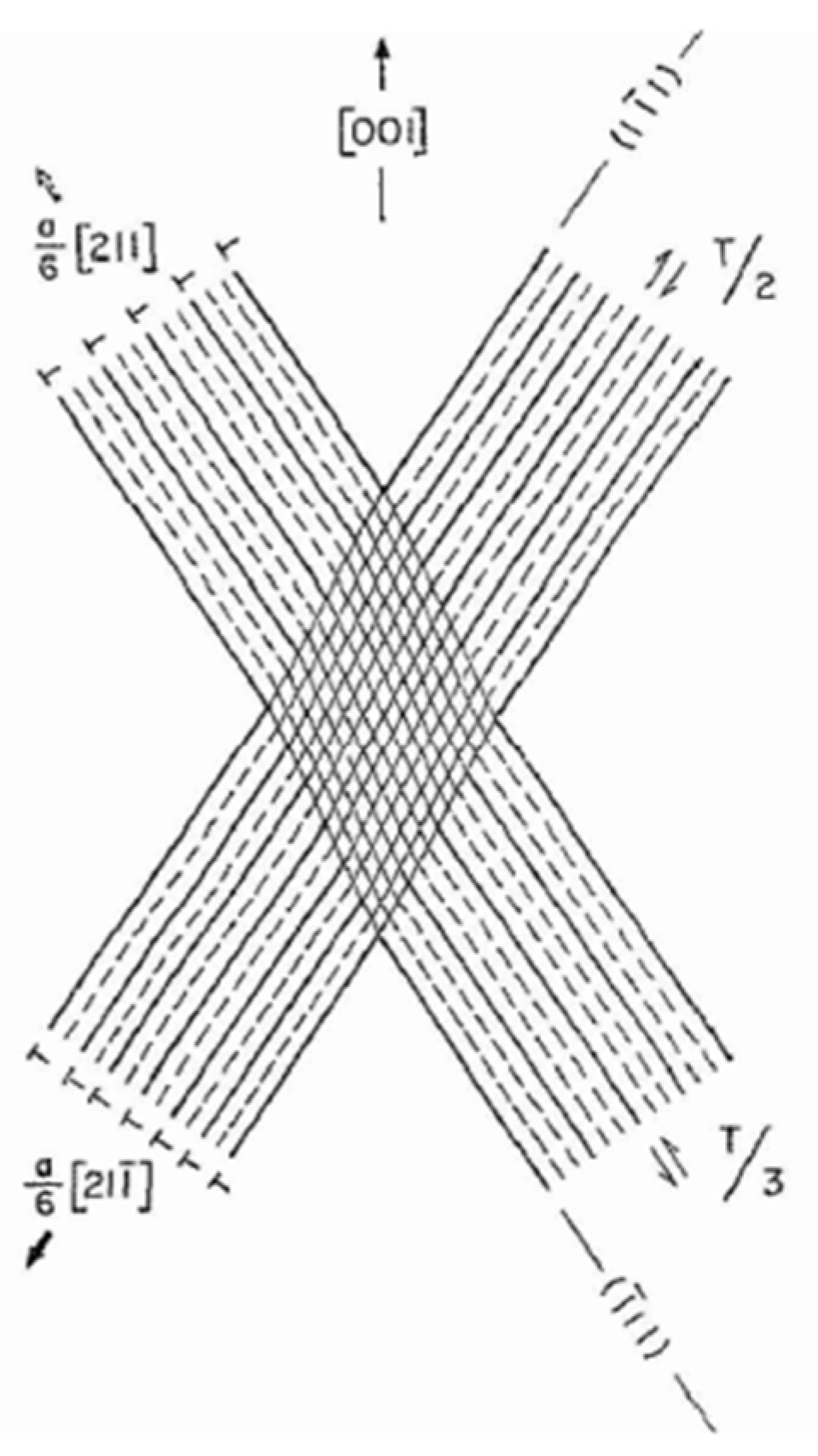
Bogers and Burgers’ work was later corrected and refined by Olson and Cohen in 1972 and 1976, with the introduction of two shears [56,57]. It can be summarized in Figure 7 as follows: the first shear on a {111}γ plane is achieved by 1/6 <112>γ partial dislocations, averaging one over every second (111)γ slip plane, and the second shear along another {111}γ plane is achieved by 1/6 <112>γ partial dislocations averaging one over every third (111)γ slip plane. The former is noted T/2 and the latter T/3. This approach is in qualitative agreement with the observations of the martensite formation at the intersection of hcp plates or stacking faulted bands on two (111)γ planes. The model has an interesting physical basis, but its intrinsic T/2 and T/3 asymmetry between the {111}γ planes seems to be too strict to be obtained in a real material. The refined model is quite complex, and does not answer anymore the question about the atomic trajectories. It also raises questions about the origin of the partial dislocations, but we will come back on this point in the next section.
Another hard-sphere model of fcc-bcc transformation was proposed by Le Lann and Dubertret [58]. This model contains some essential ingredients, such as the fact that one of dense directions remains invariant <110>γ = <111>α, and the authors qualitatively envisioned the transformation as a wave propagating perpendicularly to this direction. In addition, the authors proposed atomistic structures of the well-known {225}γ and {3,10,15}γ habit planes. However, the model seems to be widely ignored, probably because it is quite difficult to understand, as it implies the distortion of a regular octahedron made of 19 atoms, and is mainly geometric; it does not explain how to calculate the atom trajectories or the distortion matrix.
More than 150 years after Mügge’s model of deformation twinning, and more than 60 years after the birth of PTMC, the exact continuous paths related to the collective displacements of the atoms during the lattice deformation remain beyond the possibilities of the classic crystallographic theories of displacive transformations in metals. We think that the absence of progress should be attributed to the main paradigm, i.e., the assumption that the lattice distortion should be a shear or a composition of shears.
4. Simple Shear Saved by the Dislocations/Disconnections?
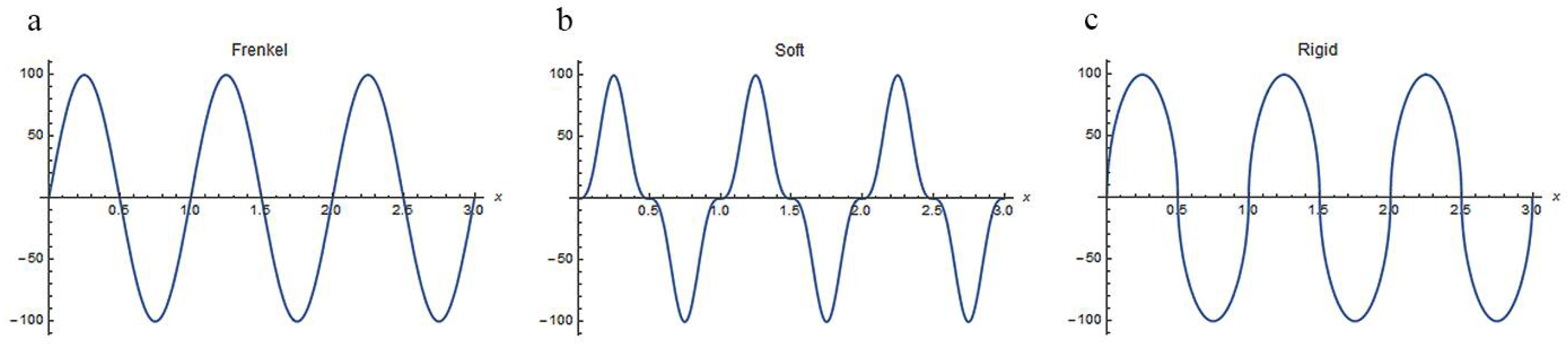
Simple shear, or its derivative lattice invariant strain, is perfectly adapted to model the collective displacements of the atoms that move all together at the same time. However, simple shear has raised important issues for a long time. Atoms are not bricks that can glide onto themselves, as represented in Figure 1. A collective shear displacement of the atoms would imply a magnitude of shear stress to the same order as that of the Young modulus. It is worth recalling the usual “demonstration” that was given by Frenkel [59] in 1926 and reported in different books [60,61]. For example, in [60], it is explained that “The shearing force required to move a plane of atoms over the plane below will be periodic, since for displacements x < b/2, where b is the spacing of atoms in the shear direction, the lattice resists the applied stress but for x > b/2 the lattice forces assist the applied stress. The simplest function these properties is a sinusoidal relation of the form , where is the maximum shear stress at the displacement = b/4. For small displacements the elastic shear strain given by x/a is equal to from the Hooke’s law, where is the shear modulus, so that and since b ≈ a, the theoretical strength of a perfect crystal is of the order of .” The sinusoidal form was also used by Peierls in his famous paper introducing the friction force on a dislocation [62]. However, Frenkel’s demonstration is actually misleading. Indeed, there is no reason to believe that the periodicity along the x-axis could explain the stress value at x = 0. What could justify that the value is correlated to the maximum value ? Actually, the “trick” of the demonstration is hidden in the sinusoidal function. This function seems to be harmless, but it already contains the answer, because it is such that its derivative is proportional to its maximum. Other periodic functions lead to completely different results. Let us consider, for example. The soft and rigid functions defined as follows:
The sinusoidal function, and the soft and rigid functions are shown in Figure 8.
The soft case gives , and the rigid case gives . In these two extreme cases, there is no correlation between the shear modulus μ and the maximum stress . One could also find different functions for which the shear modulus is constant but the maximum shear stresses are very different. Since the result is given with the premise, Frenkel’s demonstration is biased; any argument based on the periodicity of the structure cannot be correct. Cottrell mentions in the first chapter of his excellent book [54] that Orowan told him in a private communication that “the critical shear strain should be less than this when a realistic law is taken for the force between the atoms”. Cottrell then made a rough estimation using a central law force, and came to estimate this strain to be about μ/30. He also gave the advice that “the sinusoidal function [..] should be replaced by a [central force] relation”. However, he did not specify that the periodicity argument should be definitely discarded. Despite Frenkel’s error, and as shown by Cottrell, it is correct to assume that the maximum shear stress associated with a simple shear is a tenth the order of magnitude of the shear modulus. Nabarro [63] also took a more appropriate function, as suggested by Cottrell, and showed that the order of magnitude of the friction force estimated by Peierls is correct. The fundamental reason is not the periodic nature of the lattice, but the fact that the interactions between atoms located in the neighbored unit cells create a lattice friction. This can be understood by considering the case of a one-atom unit cell of Figure 9a, for which the atom interaction is assumed to be fully elastic.
If the trajectory of the atoms could continuously follow a simple shear strain, they would interpenetrate so much that the repulsive force at the interface would reach very high values. In the 2D example of Figure 9a, by noting the diameter (d) of the atoms, the rate of interpenetration would be , i.e., far above the usual elastic limit (around 0.1–1%). In the three-dimensional (3D) case of an ABCABC stacking, the layers are separated by a distance of , and a simple shear displacement of the atoms of the upper layer relative to the two atoms of the lower layer would reduce the distance between them down to , which induces an interpenetration of . Here again, this value is too high to be compatible with the elastic limits of the metals. Thus, even if incorrectly demonstrated by Frenkel (at least the sinusoidal function should be replaced by a more realistic function, as suggested by Cottrell), it is not possible, with reasonable stress, to induce a collective movement of the atoms on a crystallographic plane. This result was confirmed with the experiments made by Bragg and Lomer with sub-millimeter soap bubble rafts [64]. Please note that the real argument is the atom size/interatomic energy, and not the lattice periodicity. The hard-sphere assumption is a rudimentary expression of the interatomic energy. Similar calculations can also be applied to metallic glasses, despite their quasi-amorphous state.
Anyway, the conclusion seems unescapable: the stresses that would be required to shear a perfect crystal are far too high. Dislocations are thus required for any shear deformation, whether by gliding, twinning, or martensite transformation. Dislocation theory was emerging, and was soon successful in 1940–1950 in explaining the plasticity of metals, recrystallization, and many other phenomena in materials science. Brilliant confirmations of the existence of dislocations were also obtained by TEM in the early 1950s [65]. Consequently, most of the researchers came to assume that dislocations were the cause and the most fundamental part of deformation twinning. According to Hardoin Duparc [4], the term “twin dislocation” was coined by Seitz and Read in 1941 [66], and this concept has been pursued till now by Vladimirskii [67], Frank and van der Merwe [68], Sleeswyk [69], Christian and Mahajan [2,70], and many other great scientists. Let us cite Cottrell [54] when he explains the arguments and the reasoning at the origin of the concept of twinning dislocations. “It has often been suggested that mechanical twinning takes place by the continuous growth on an atomic scale of twinned materials, and the general arguments for a dislocation mechanism are the same as in the case of slip; first, it is scarcely believable that the atom should all move simultaneously and, second, twinning occurs at stresses comparable with those for slip, i.e., far below the theoretical strength of the perfect lattice.” Please note that it is supposed that all the atoms move simultaneously, i.e., all at the same time—but we will come back later on this point. Cottrell continues directly, by proposing a first version of what will become the “pole mechanism”:
Frank and Read’s model, mentioned by Cottrell, was explained a little earlier in his book; it is a former model of what is now known as “Frank–Read” source of dislocations. In this model, Frank and Read imagined a dislocation rotating around a point, producing a new slip for each revolution, as explained by Cottrell in the Figure 49 of his book [54] reported in Figure 10a,b. Cottrell made a parallel with the spirals formed at the surface of a growing crystal, even if it was clearly stated that this spiral dislocation results from growth and not from deformation. The Frank-Read model used by Cottrell to explain twinning was the ancestor of the “pole mechanism” model. It was followed by Cottrell and Bilby’s model [71], refined by Sleeswyk [69,72] and again later by Venables [73] (Figure 10c). Sleeswyk [69] also imagined how the twinning dislocations at the interface could dissociate at the interface and move away, and he introduced the concept of “emissary dislocations”. General considerations on twinning mechanisms and twinning dislocations in metals can be found in Ref. [2,3]. An updated review was recently published by Mahato et al., in Section 4 of [74].Since a new configuration is produced by twinning, the dislocations that cause it must be imperfect. While it is usually not difficult to discover a suitable imperfect dislocation to cause the required shear of neighbouring planes as it passes between them, the problem is to explain how twinning develops homogeneously through successive planes. The homogeneous shear required a twinning dislocation on every plane without exception, which seems unlikely, or the motion of a single dislocation from plane to plane in a regular manner. Cottrell and Bilby have recently suggested a mechanism, based on that of Frank and Read, whereby the latter process can occur in certain crystals containing dislocations. Figure 51 [reported in Figure 10b] illustrated the mechanism. Here OA, OB, and OC, represent three dislocation lines and CDE is a slip or twinning plane. The dislocation OC (“the sweeping” dislocation) and its Burgers vector both lie in this plane (the “sweeping” plane) and the dislocation can rotate in the plane about the point O. If it is a unit dislocation and remains in the plane as it rotates a slip band is formed. The requirements for twinning (or a shear transformation) to occur are as follows: 1. The sweeping dislocation must be imperfect and produce the correct shear displacement on the sweeping plane; 2. Successive sweeping planes must be joined to form a helical surface.[54]
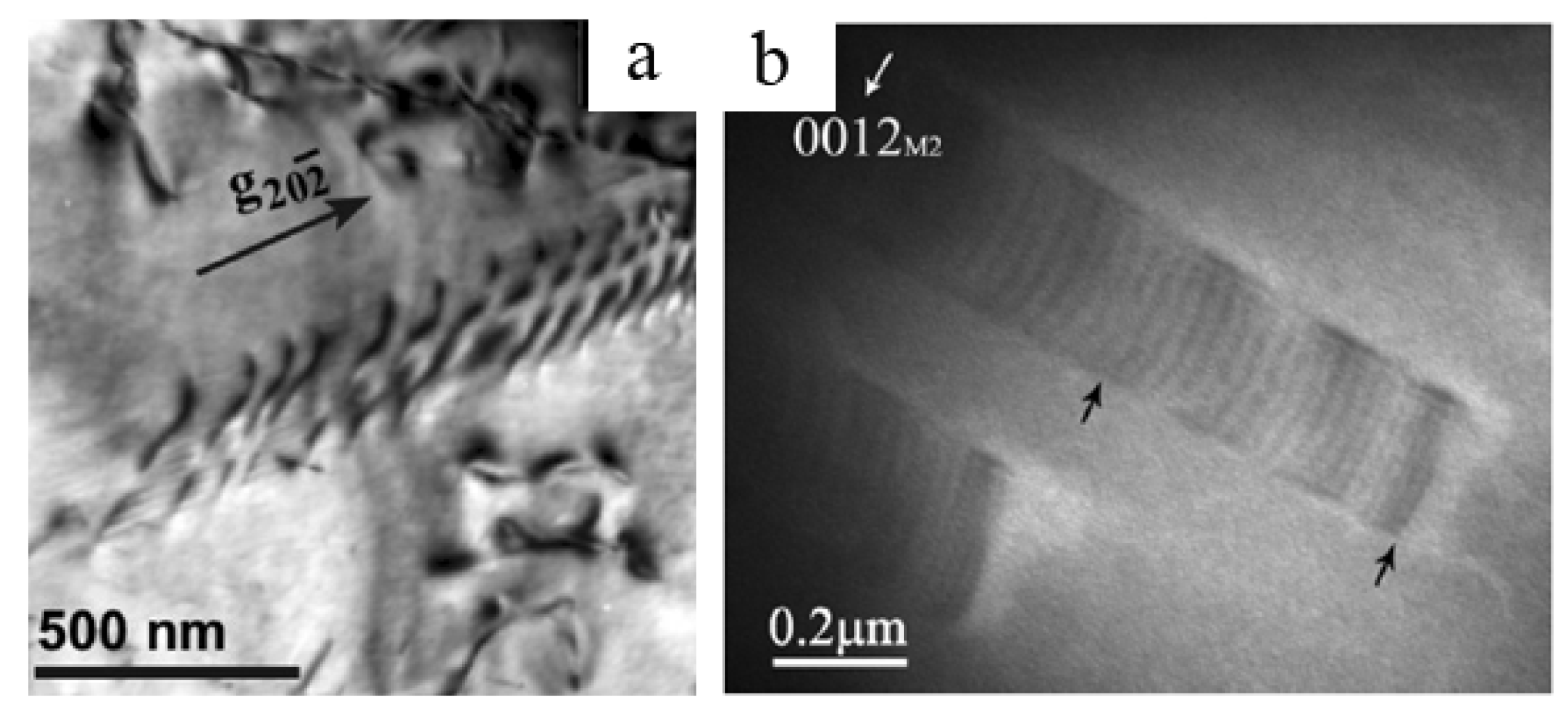
TEM observations confirmed the existence of dislocations, dislocation pile-ups, dislocation dissociations, climb, etc. However, to our best knowledge, the spiraling dislocations that should be expected from a pole mechanism have never been proven in metals. Spiraling/helical dislocations were observed by TEM in cast Al–Cu alloys [75], but they come from a vacancy collapse and not from stresses. What are often presented as TEM images of “twinning dislocations” are dislocation pile-ups in front of micro-twins [74,76,77,78,79], such as those shown in Figure 11. They are generally interpreted in term of dissociations of full dislocations associated with complex pole mechanisms; however, to the best of our knowledge, the initial spiraling dislocation source has never been shown.
The notion of “twinning dislocations” has been progressively enlarged to displacive phase transformations. For fcc-hcp and hcp-fcc transformations, the classical models imply the coordinate displacement of partial Shockley dislocations, which are supposed to be created by a pole or similar complex mechanism [80,81,82,83]. For fcc-bcc transformations, we have seen in Figure 7 that Olson and Cohen [56,57] used partial dislocations in order to correct the initial hard-sphere Bogers and Burgers model [53]. The use of dislocations as a fundamental part of the transformation models was generalized with the introduction of the concept of “disconnection”, which became the core of the “topological model” (TM) developed by Hirth, Pond, and co-workers [84,85,86,87,88]. A disconnection is a kind a dislocation located at the interface of two misoriented crystals, which can be of same phase (for twinning) or different phases (for phase transformation)—it is the assembly of a classical dislocation and a geometrical “step”, both required to assure the compatibly at the interface. The dislocations/disconnections are assumed to be glissile, because twinning and martensitic transformations are envisioned as the consequence of the propagation of the interface, and researchers came to introduce the concept of “glissile interfaces” [70] by extrapolating the concept of glissile dislocations. Despite its efficiency in describing locally, at a nanometer scale, the structure of the interface between the parent matrix and the daughter crystal, the TM does not answer yet the most important questions: where the dislocations come from? How are they created? How can they move collectively and in coordinate way to build a new phase? How can they move at the sound velocity? Why is twinning activated when the temperature decreases? Why do hcp metals exhibit so many twinning modes with so few dislocation modes? Atomistic simulations [89,90] show that some dislocation loops can be created “ex-nihilo” (helped by the external stress field and dislocation pile-ups) and that these loops can be the very first nucleation step of twinning. These studies propose partial responses to the first two questions, but the others remain open.
5. Angular Distortive Transformations
5.1. Twinning Dislocations Replaced by Transformation Waves and Dislocations Induced by Twinning
Let us now explain the way we envision deformation twinning and martensitic transformations. The TEM images of the dislocation pile-ups in front the micro-twins, such as those of Figure 11, do not prove that the dislocations are the cause of twinning; they may be as well a consequence of twinning. Despite the fact that for the last 60 years, nearly all the theoretical models and experimental observations have been interpreted in terms of twinning dislocations or disconnections, it is difficult to believe that dislocations could be created in a periodic sequential way by a pole mechanism, and that they could propagate at the speed of sound and produce a new crystallographic structure (twin or martensite). The high speed of twin/martensite propagation, and the fact they are favored by low temperatures and high deformation rates, should constitute important arguments against theories based on dislocations. Cottrell is right when he says that “it is scarcely believable that the atom should all move simultaneously” [54], because that would imply that all the bonds break instantaneously, which would require very high energy for an instantaneous moment. Nevertheless, an important point should be considered: in non-quantum physics, the word “instantaneously” has no meaning. Information cannot travel faster than a limited speed, i.e., the speed of light for electromagnetism, or the speed of sound for waves in materials (even if supersonic dislocations are reported for extreme conditions). Let us explain this general idea with the classical Ising model. Reversing a spin has an influence on the neighboring spins, and when the temperature is close to the transition (Curie) temperature, i.e., when the local spin–spin interaction energy is not masked by the high temperature Brownian motion, nor counterbalanced by the low temperature global magnetic field, this influence becomes predominant on the system, and the magnetic susceptibility and the correlation length become infinite [91]. The effect of flipping a spin on the other spins is not instantaneous, but travels at the speed of light. The spin-up and spin-down domains are thus not formed instantaneously; they appear under the effect of a solitary phase transition wave, i.e., a soliton. It can be imagined as a domino cascade or as a seismic wave. This idea is not new, but it has appeared only sporadically in metallurgy literature, with long periods of oversight. Machlin and Cohen [42] envisioned martensitic transformation in Fe–30Ni alloys as a strain wave; Nishiyama wrote in his book that “martensite transformation is like Shôgidaoshi (a Japansese word meaning ‘falling one after another in succession’) rather than like military notion” [37]. Meyers [92] proposed an equation of martensite growth that takes into account the velocities of the longitudinal and shear elastic waves. Le Lann and Dubertret [58] developed their crystallographic model of fcc-bcc transformation by maintaining the direction <110>γ = <111>α invariant, because they considered it to be the wave vector of the transformation. With this method of envisioning displacive phase transformations, there is no need of dislocations, at least not in a free single crystal. In 1984, Barsch and Krumansl introduced the concept of a soliton creating boundaries without interface dislocation for ferroelastic transitions [93,94]. Solitary waves were also introduced by Flack in a one-dimensional shear model [95]. Unfortunately, there are few works in metallurgy based on this physical idea. A Russian team lead by Kashchenko and Chashchina [96] are developing the concept of dynamics and wave propagation of martensite in steel, but the physical details (l-waves, s-waves) are not easy to understand for a non-physicist, and would need experimental confirmations.
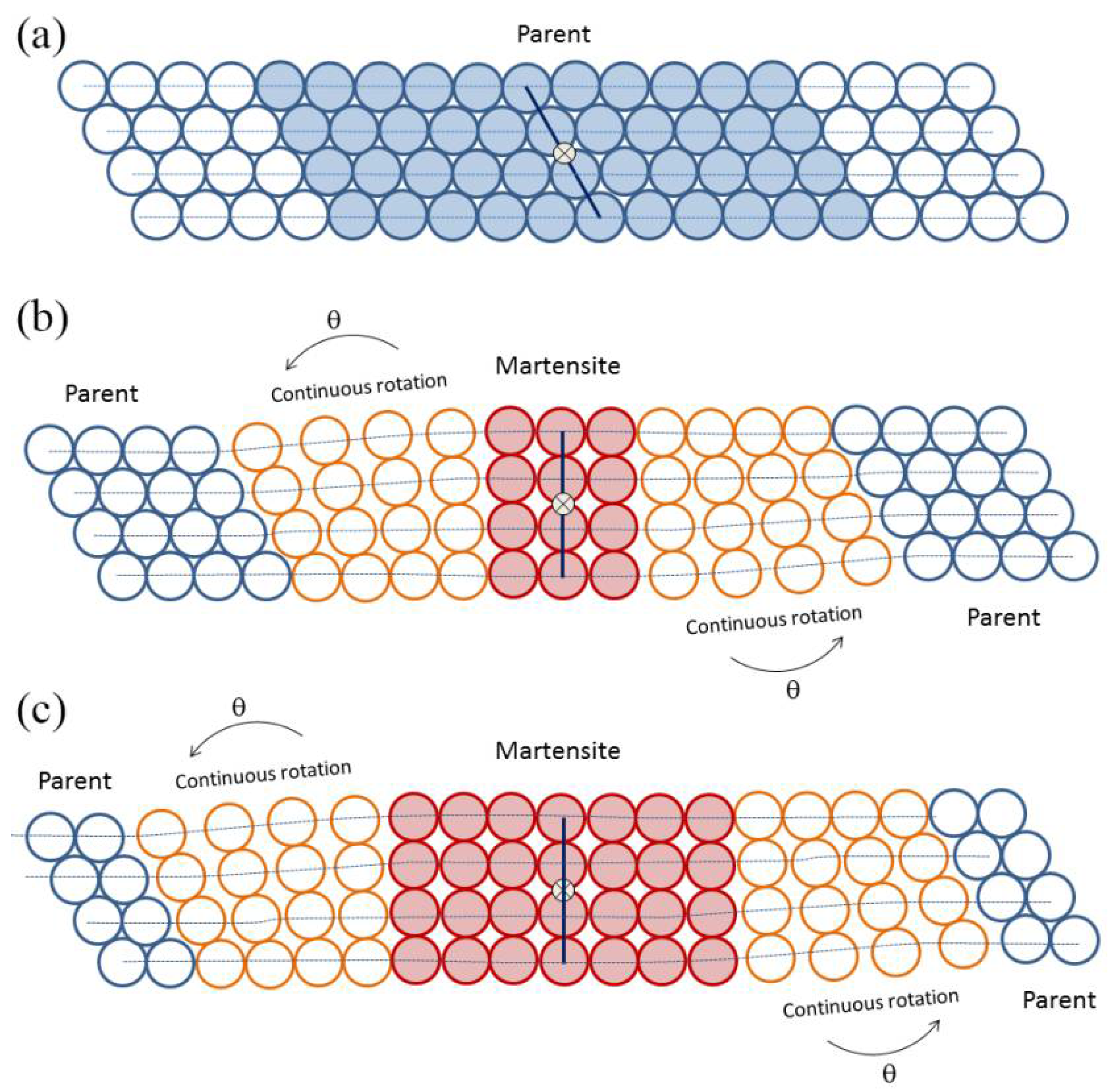
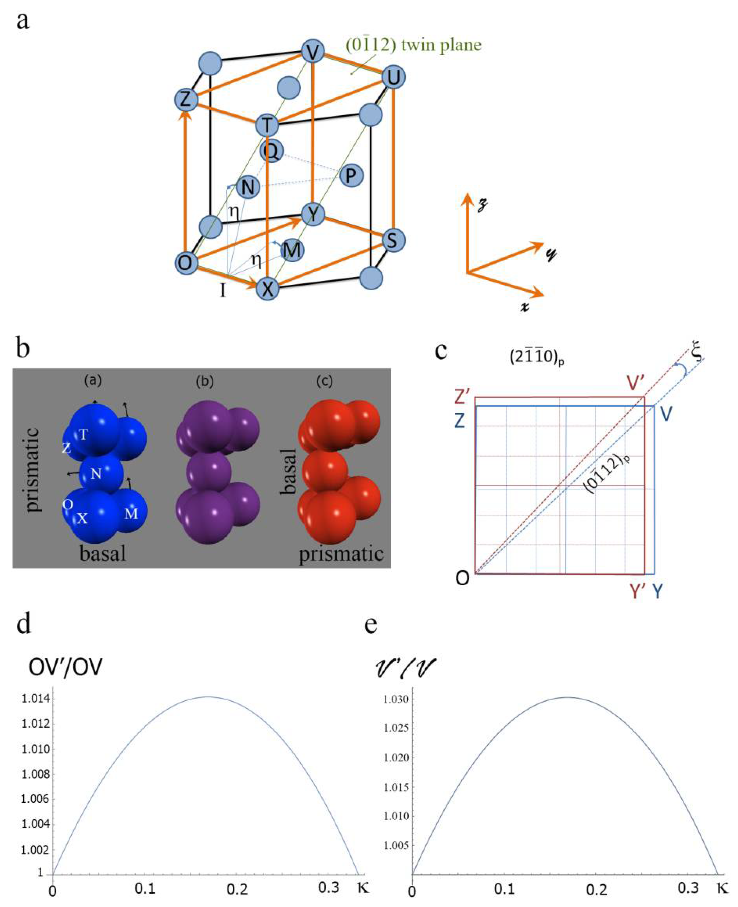
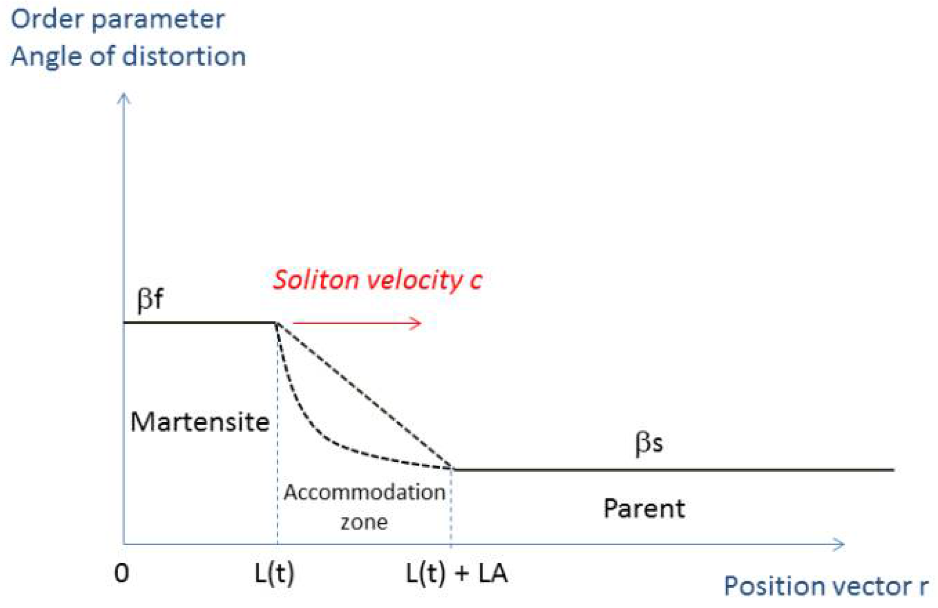
We consider here that during deformation twinning or martensitic transformation in a free crystal, the atoms move following a solitary “phase transformation wave”, i.e., a phase soliton, as geometrically shown in Figure 9a and Figure 12.
The displacement of each atom has an influence of the neighboring atoms, the way that a spin flip has an influence of the neighboring spins in an Ising model. If the parent single crystal is free, the lattice distortion becomes a macroscopic shape distortion. This idea is quite new to us, and should be developed; however, it seems possible that the parent/martensite accommodation area, in orange in Figure 12, is spread over a large area, such that the distances between the neighboring atoms remain lower than the limit imposed by the critical yield strain, and the interface is accommodated purely elastically. Such a model will be detailed in the last section. There is no reason to believe that the dislocation-free model proposed by Barsch and Krumansl is limited to ferroelastics. For polycrystalline materials or non-free crystals, one must distinguish two cases, depending on the martensite size. When the size of the martensite domain and its elastic accommodation zone are significantly lower than the grain size, the distortion can still be elastically accommodated inside the grain, at least during high-speed transitory stages of the transformation process. The elastic zone is then quickly relaxed by the formation of dislocation arrays in the surrounding matrix, and by interfacial dislocations (disconnections). When the martensite grows and the size of the elastic accommodation zone becomes comparable with the grain size, the incompatibilities must then be plastically accommodated, as schematized in Figure 13. The volume change associated with the phase transformation is averaged in all the grains, and distributed in a whole sample (it can be measured by dilatometry), but the deviatoric parts of the lattice distortion are “blocked” by the grain boundaries. The accommodation zone cannot be spread any further, and dislocations become necessary.
5.2. The Concept of Angular Distortion
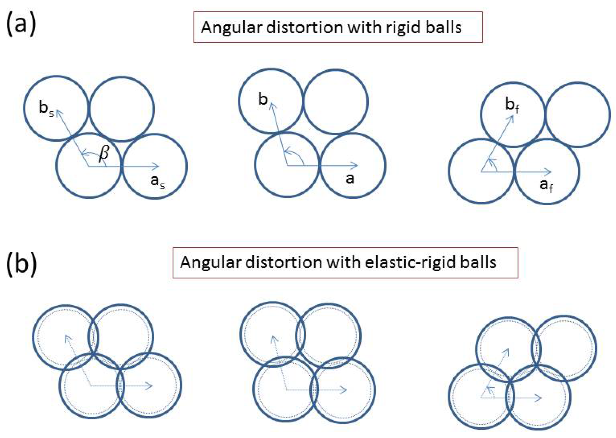
Freed of the limitations imposed by the shear paradigm and the associated twinning dislocations, one can now imagine how the atoms move during displacive transformations. Of course, atoms are not hard spheres, but in some metals (fcc, bcc, and hcp with the ideal packing ratio), the hard-sphere assumption is a good starting point [8]. Simple (or pure) shears are deformation modes at constant volume, which is well-adapted for plasticity by dislocation, but is not suited for displacive transformations in these metals. Indeed, it is known from Kepler in 1611 (Kepler’s conjecture became a theorem in 1998, thanks to Hales’ demonstration) that the two densely-packed structures are fcc and hcp, which means that any intermediate state between two fcc crystals, two hcp crystals, or an fcc and a hcp crystal should have a higher volume than that of an fcc or hcp crystal. Simple shear is not compatible with the hard-sphere assumption if one is looking for continuous deformation models. Let us look again at Figure 9a. When a simple shear is applied continuously to a crystal, the distance h between the atomic layers is supposed to be constant, as if the crystal were constrained between two infinitely-rigid horizontal walls. Now, with a hard-sphere model, we consider the case in which the crystal is free to move in the direction normal to the atomic layers, as illustrated in Figure 9b and Figure 14a. Of course, the atoms can slightly interpenetrate each other according to a reasonable elastic limit (that should be defined), but on first approximation it is assumed that the sphere size is only slightly elastically relaxed, such that the trajectories of the atoms are the same as those of hard spheres (infinitely rigid) with a slightly lower diameter than the initial one, as shown in Figure 14b.
Thus, on first approximation, the atomic displacements are not essentially modified by the elasticity of the spheres; the trajectories remain close to that of “rolling balls”. Now, if the lattice noted by the vectors (a, b) in Figure 14a is considered, the distortion is no longer a simple shear along a; it is a distortion in which the length of the vector b remains constant (it is and remains the atom diameter), and the angle between the vectors a and b, noted here as β, continuously changes. This angle becomes the unique parameter of the lattice distortion; in physics we would say that it is the order parameter of the transition. The trajectories of the atoms naturally become arcs of a circle, and the lattice distortion is not a shear strain anymore, but an angular distortion. With such a simple approach, the shape of the crystal is given by the same distortion as that of the atomic displacements. Of course, in polycrystalline materials, a grain is not free to arbitrarily deform, due to the surrounding grains, and complex accommodation modes by variant coupling and by dislocations are required.
5.3. Accommodation Dislocations and Disclinations
The accommodation dislocations are not randomly distributed; they are such that their strain field compensates for the deviatoric parts of the angular distortion, and constitute the plastic trace of the mechanism. In our opinion, these dislocations are those shown in the TEM images of Figure 11. The elastic field associated with the dislocation arrays should be equal to the back-strains between the martensite product and the parent crystal. These dislocation arrays are very probably at the origin of the continuous features observed in the Electron Back Scatter Diffraction (EBSD) pole figures of martensitic steels (see next section). It can be expected that for soft parent/hard daughter phases, the distortion is accommodated inside the parent phase; for hard parent/soft daughter phases, the distortion is accommodated inside the daughter phase, and one can expect an equal proportion for deformation twinning. According to this model, the mesoscopic strain field should be dictated by the phase transformation distortion, and the exact and detailed knowledge of the structure of the dislocations adopted by the material to produce this strain field is not required to explain it. As the lattice distortion is now modelled by an angular distortion, the dislocation arrays should be formed in order to compensate for the angular deficit (or excess) implied by the distortion. The most appropriate plastic mode for such types of accommodation implies the concept of “disclination”. This concept was first introduced in 1907 by Volterra [97], who considered two types of defects in a periodic solid: the rotational dislocations (disclinations) and the translational dislocations (simply referred as dislocations nowadays). The disclination strength is given by an axial vector w, called the Frank vector, encoding the rotation needed to close the system in a similar way that the dislocation strength is given by its Burgers vector b, encoding the translation needed to close the Burgers circuit. If dislocations constitute a fundamental part of metallurgy, disclinations are less known. The theory has been developed by Romanov [98], and by Kleman and Friedel [99], but the applications are mainly limited to highly deformed metals [100]. To our knowledge, only Müllner and co-workers use disclinations to calculate the strain field and strain energy of hierarchically twinned structures formed by deformation twinning [101] and by martensitic transformation in Ni–Mn–Ga Heusler alloys [102]. Their models are based on the classical concept of shear, but it could of interest to see if the classic concept could be substituted by that of angular distortion. The disclinations shown in Figure 15 would be the natural accommodation modes of positive or negative angular misfits.
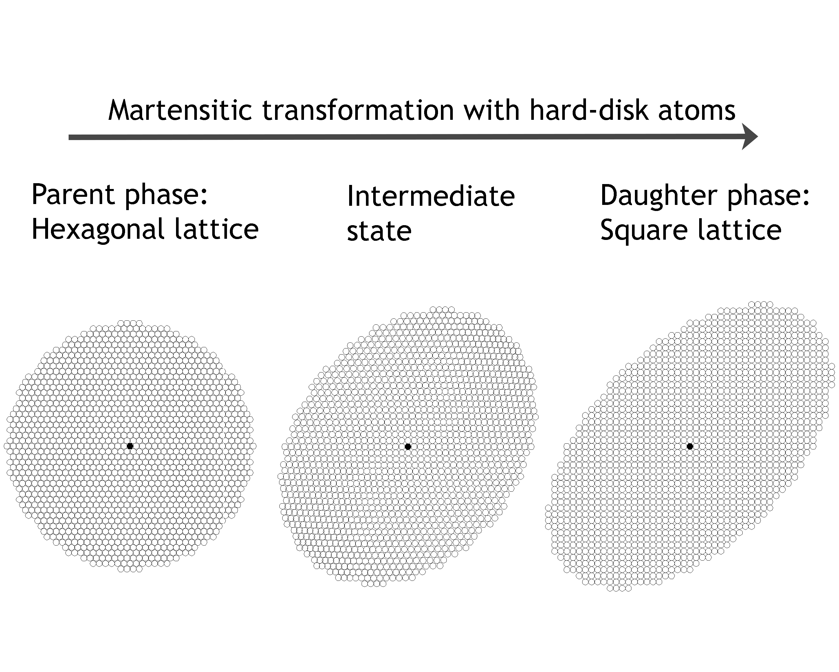
In this approach, martensitic transformations and deformation twinning are not the result of a cause that would be the sweep of “twinning dislocations”, or of the propagation of a “glissile interface”; instead, they directly result from a lattice distortion, whose driving force is (a) for martensite, the difference of chemical energy between a parent phase and its daughter phase; and (b) for twinning, the difference of mechanical energy given by the work of the applied stress along the distortion path. The interface and accommodating dislocations in its surroundings then appear as the consequences of the distortion. Large volumes of parent phase are suddenly transformed into daughter phase (at the acoustic wave velocity), and the parent–daughter interface created by the distortion is made of glissile and sessile dislocations/disconnections. At mesoscale, these dislocations induce rotation gradients (disclinations), such as those schematically represented in orange in the hexagon–square transformation of Figure 12. This way of envisioning deformation twinning and martensite transformation completely reverses the usual paradigm, which gives a central driving role to the dislocations in the transformation mechanism. There is no need here to imagine a hypothetical complex pole mechanism, because the dislocations are now created by twinning or by martensitic transformation; similarly, there no need to impose glissile properties to the interface. It is true that plasticity is required to accommodate the lattice distortion in polycrystalline metals; however, in no way does that mean that dislocations/disconnections are the cause or can explain the distortion.
6. Angular Distortion versus the Phenomenological Theory of Martensite Crystallography, Illustrated with a Simple Example
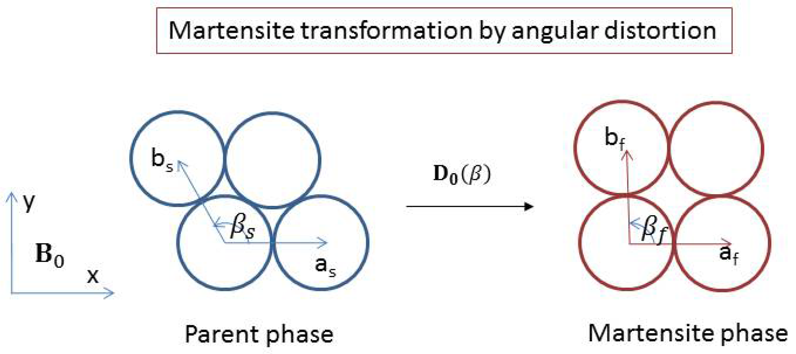
The concept of angular distortion is so simple and natural that it can be directly applied to martensitic transformations, without requiring the four (or more) matrices of the PTMC. Let us use again the example of a 2D hexagonal–square phase transformation of Figure 12. The classical PTMC decomposes this transformation into two distinct paths. The first path is the matrix product R.U, which says that first a (Bain) stretch U is applied, and then a rotation R must adjust the stretch in order to maintain an invariant line (here the x-axis). The notation U is now preferred to B (Bain) to avoid confusion with our notation of the bases. The second path is P1.P2, where P1 is an IPS and P2 a simple shear. Here, P2 is reduced to the identity because only P1 is required to get the final square lattice. However, even by keeping only P1, one must admit that the case is not direct, because there are two parameters in P1—i.e., the simple shear Ps and the dilatation Pδ (see Figure 5a). The directions of the vectors s and δ are known, but nothing is said on how the norms of these two vectors evolve during the transformation. The PTMC treats the two paths R.U and PsPδ as two independent steps, as shown in Figure 16. One can understand with this simple example why PTMC is still phenomenological and continues to be mute on atomic displacements during the transformation, even seventy years after its birth. Do the atoms follow the trajectory R.U or the trajectory PsPδ? Only an atom with a gift of ubiquity or behaving as a quantum particle could follow both paths at the same time. The only way to tackle this issue is to impose rules between the parameters involved in R, U, Ps, and Pδ, such that an equality of the two paths is obtained during the transformation for all the intermediate states. These calculations will be given a little later in the text.
Now it is easier to directly propose our alternative to the PTMC. The trajectories of the atoms can be determined by using an angular distortion matrix. The only thing to do is to write the way that the lattice is distorted by the atomic displacements. In that aim, we use the crystallographic basis and the orthonormal basis . During the distortion, the vector a remains invariant, and the vector b is rotated. Its image is noted b’. The angle between a and b’ is β. The angle β decreases during the transformation; it is in the starting state, and it is in the final state, as shown in Figure 17.
The vectors define a crystallographic basis expressed in by
The matrix of lattice distortion between the starting basis and any distorted basis , expressed in the crystallographic basis , is simply = . This matrix can now be expressed in the orthonormal basis by using the usual coordinate change equation, i.e., . It then becomes
This equation is very general and can be applied to any displacive transformation. In the hexagon–square example, combined with Equation (2), it directly gives
The matrix of complete distortion is obtained for :
The volume (here, surface) change during the distortion is given by the determinant of the distortion matrix:
We take the opportunity given by Formula (6) to mention an important point. It was assumed by Weschsler, Liebermann, and Read in their seminal paper [33], which gave birth to PTMC, that the average distortion matrix D resulting from two distortion matrices D1 and D2 of variants in proportions and , with 0 ≤ λ ≤ 1 is
This formula only works in the special condition called “kinematical compatibility”; in the general case, the volume is not conserved, i.e., . We note that, to the best of our knowledge, Bowles and Mackenzie never used this formula, and they always composed matrices by multiplication. That is why we are not convinced when it is said that the Wechsler et al. and Bowles and Mackenzie forms of the PTMC are similar; they differ at least in the way the distortion matrices are averaged. This is probably one of the reasons why both PTMC versions have continued their own developments without intermixing, nearly ignoring each other.
The approach based on hard spheres is very effective in comparison with the PTMC, because it gives in one simple step the continuous analytical expression of the lattice distortion that is compatible with the atom size, and is thus realistic from an energetic point of view. The PTMC can determine the distortion matrix only once the transformation is finished, i.e., Equation (5). Of course, one could try developing a complex continuous infinitesimal version of the PTMC, as in [103], but the method is artificial and needlessly heavy. For example, let us come back to 0, and try to find the expressions R, U, Ps, and Pδ such that the two paths are maintained equal during the transformation. We note O, A, B, and C as the nodes of the lattice, with the vectors OA = [1,0], , and . The stretch component in a local orthonormal basis positioned along the diagonal OC and AB is
This local basis is obtained from the reference basis by a rotation of angle . Thus, the stretch distortion matrix in the basis is
The compensating rotation matrix R is a rotation of angle
The other path of the PTMC is made of the shear displacement along the x-axis of the point B, located at a distance h from the shear axis. For a simple shear, h is constant and equal to . Thus
The second part of the second path is an extension along the y-axis that dilates the distance h and makes it become . The dilatation matrix is thus
The first path is continuous, and its analytical expression is given by the product with the matrices given in Equations (9) and (10). The second path is continuous, and its analytical expression is given by the product with the matrices given in Equations (11) and (12). The atoms do not need ubiquity anymore, because the reader can check that the two paths are actually equal: the path corresponding to the angular distortion given by Equation (4). We let the reader make his own opinion on the physical relevance and simplicity of Figure 17 and Equation (4), and that of Figure 16 and the set of four Equations (9)–(12).
7. The Angular Distortive Model for Face-Centered Cubic–Body-Centered Cubic Martensitic Transformation
7.1. The Intriguing Continuities in the Pole Figures
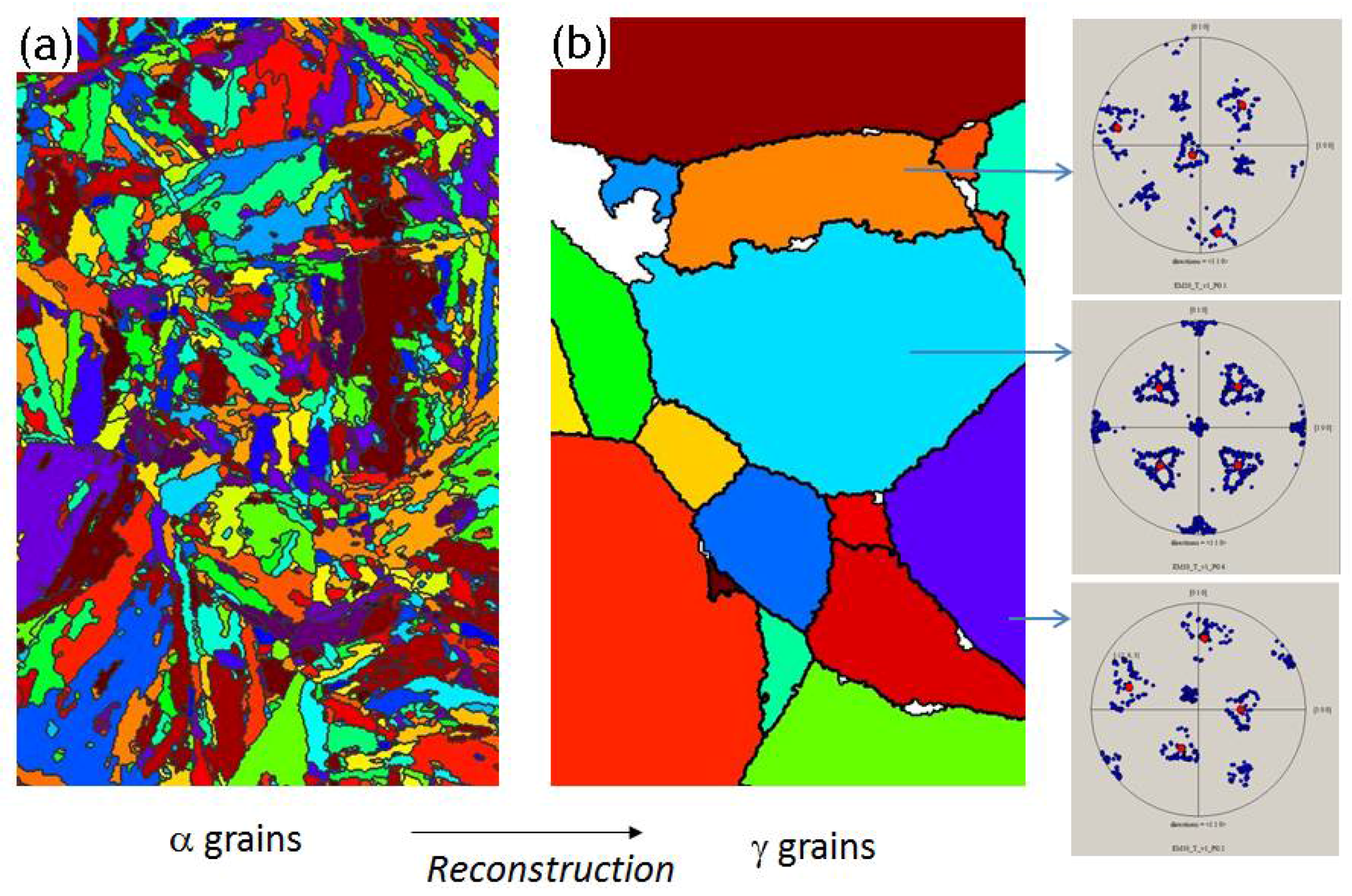
When fully transformed, many steels and titanium or zirconium alloys are only constituted of the daughter phase, without a sufficient amount of retained parent phase to know the sizes and orientations of the prior parent grains that had existed at high temperatures before the transformation. This apparently lost information is, however, crucial to get a better understanding of the fatigue, impact, and corrosion properties, because the prior parent grain boundaries are preferential location sites of impurity segregation. A method to reconstruct the prior parent beta grains in titanium alloys from EBSD maps was proposed by Gey and Humbert [104], but at that time it was based on misorientations between grains and was not applicable to steel, due to the highest number of symmetries and variants. New constraints had to be found to reduce the influence of the tolerance angle. These constraints were found in the algebraic structure of variants. The orientational variants and their misorientations form a groupoid [105], and the theoretical groupoid composition table can be used to automatically reconstruct the parent grains from EBSD data [106,107]. An example of reconstruction is given in Figure 18.
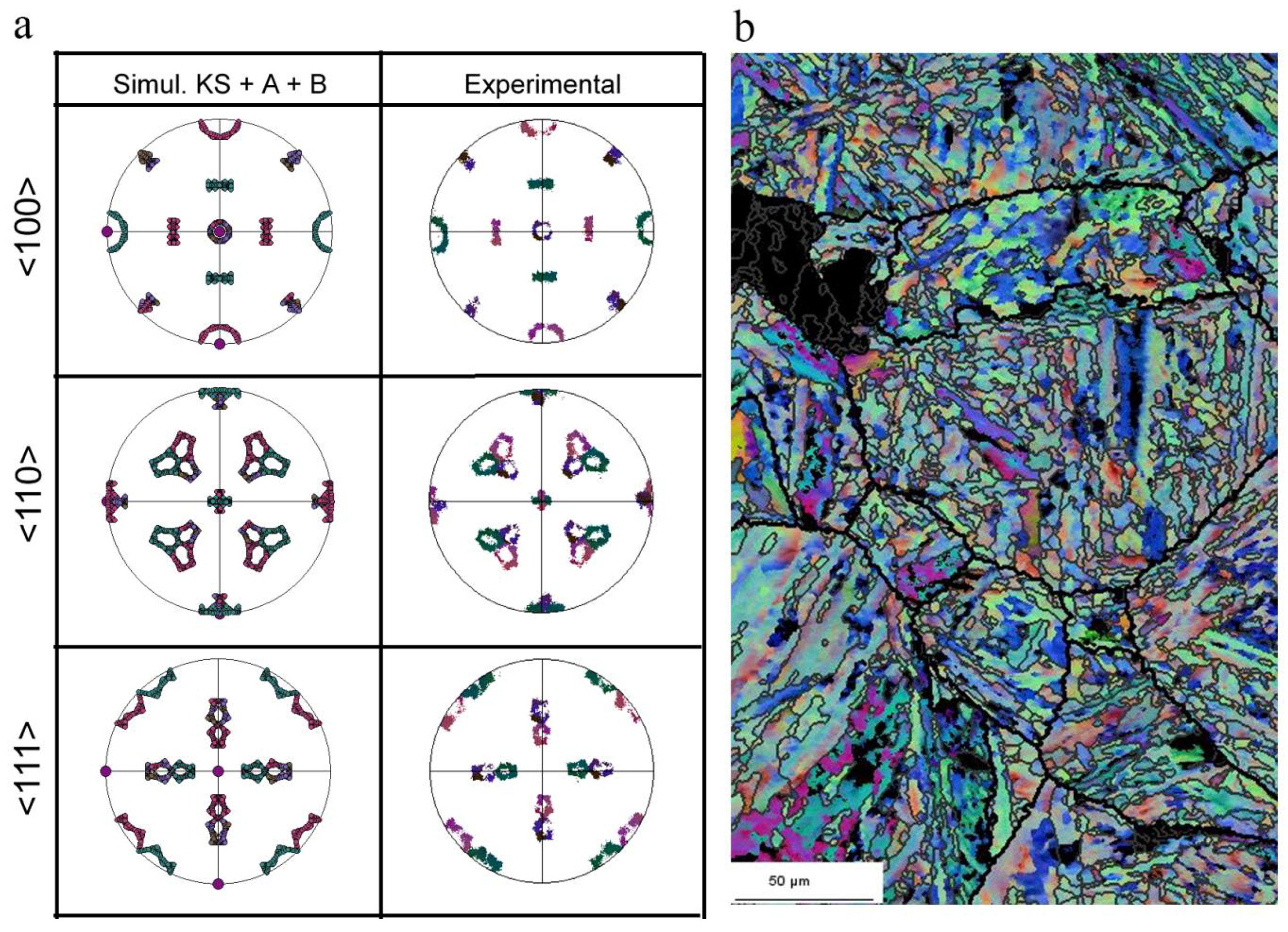
The reconstruction method was applied to many alloys, and was something striking: for low-alloyed steels, continuous features were observed in the pole figures of the martensitic grains contained in the prior parent grains. That was surprising because only a discrete distribution of orientations was expected from the 24 KS variants. As these features were observed in many different steels, and were also reported by X-ray diffraction and EBSD in Fe–Ni meteorites [108,109], we made the hypothesis that they were the plastic trace of the distortion mechanism itself. The features could be simulated phenomenologically by applying two continuous rotations A and B to the 24 KS variants, one around the normal to the common dense plane, and one around the common dense direction, with rotation angles continuously varying in the range [0°, 10°].
7.2. A Two-Step Model Developed to Explain the Continuous Features
What is the physical meaning of these rotations? The PTMC tells nothing about them, and we checked that they were not correlated to the usual plastic deformation modes of the bcc or fcc structure. We found that the rotations A and B could be associated with the fcc-hcp and hcp-bcc transformations, respectively; a two-step model was then established, implying the existence of an intermediate fleeting hcp phase, even in alloys without a retained ε phase [110]. It was later realized that this two-step model has some similarities with the initial KSN model shown in Figure 3, the first shear in the KSN model being replaced by the fcc-hcp step made by sequential and coordinate movements of partial Shockley dislocations, supposed at that time to be originated by a pole mechanism [111]. However, further investigations could not confirm the two-step model. No trace of the intermediate hcp phase could be found in the microstructures of the martensitic steels; and ultrafast in-situ X-ray diffraction experiments in two synchrotrons (ESRF and Soleil) could not put into evidence the hypothetical fleeting hcp phase [112]. In addition, the pole mechanism appeared to us more and more doubtful (see previous sections), and many questions remained unanswered. All these “negative” results prompted us to consider other models for the fcc-bcc transformation.
7.3. One-Step Hard-Sphere Model with Pitsch OR
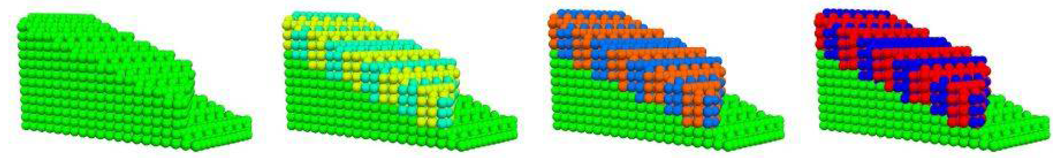
Would it be possible to establish a mechanistic model, as simple as possible, without combining shears and without dislocation in its core—a model in which the atoms would move collectively in one step? The important thing is to start the orientation relationship between the fcc and bcc phases. It was noticed that the KS, NW, and Pitsch ORs were located in the continuous features observed in the EBSD pole figures, and we made the assumption that all these ORs actually result from a unique OR, a “natural” spontaneous OR of the transformation for stress-free samples. What could this “natural” OR be? The Bain OR obtained by lattice stretching maintains the highest number of common symmetries between the parent fcc and the daughter bcc, and thus could be a good candidate if one imagines that all the chemical bonds “break” instantaneously at the same time. However, a criterion that predicts the OR only from symmetry considerations would not agree with experiments, and would probably not be relevant. Indeed, the transformation does not occur instantaneously; we envision it as a wave. The existence of common dense directions or planes obtained for special ORs, as it is the case for the KS OR, is probably favorable to wave propagation, whereas stretch distortions in general do not maintain the parallelism of dense directions. Besides any theoretical considerations, the experimentally determined ORs are more than 10° far away from the Bain OR. Could the Pitsch OR be a good candidate? This OR is less well-known than KS or NW; it was observed by Pitsch in 1959 after cooling a TEM lamella of iron nitrogen alloy [113], which means that it was formed without the surrounding stresses that exist in bulk samples. Maybe Pitsch OR was the missing link to build a theory. The Pitsch OR is at the midway between two low-misoriented KS variants, in the same way that the NW OR is at the midway between the two other low-misoriented KS variants. The simulations of the pole figures with 24 KS variants and the rotations A and B with angles limited to 0–5° are shown in Figure 19a. The distortion matrix associated with the Pitsch distortion was calculated, and the rotations A and B were qualitatively explained by the Pitsch distortion, even if the simulations were based on KS OR and not the Pitsch OR. For the calculations, the lattice parameters of the fcc and bcc phases had to be chosen, and those of hard-sphere packing with a constant atomic radius for the iron atoms were taken as a first approximation. Even if a hard-sphere model is not perfect, because the size of Fe atoms are not exactly the same in the fcc and bcc crystals (4% of difference), it is a good starting point to build an atomistic model. The Pitsch distortion matrix could be diagonalized, and the strains were surprisingly lower than those of Bain—but the basis of diagonalization is not orthonormal [114]. One year later, we developed a method to show in the EBSD maps the regions oriented according to Pitsch, KS and NW ORs with a red, green, and blue (RGB) color coding [115]. It was applied to various steels and confirmed that each bcc martensitic grain exhibits internal gradients between the Pitsch–KS–NW orientations, as shown in Figure 19b. However, the gradient NW/KS/Pitsch/KS/NW, expected by the Pitsch distortion model, could not be clearly identified, which cast doubts on the Pitsch distortion model.
Despite the absence of unambiguous experimental confirmation, we had a feeling that the fundaments of the model (one-step and hard-spheres) were correct. However, could KS, in place of Pitsch, actually be the “natural” OR? The KS OR was also reported in a quenched TEM lamella [116]. The KS OR also gives the best simulations of the continuous features in the pole figures, and is the only OR that allows the parallelism of the dense directions and the parallelism of the dense planes of the fcc and bcc phases at the same time. What if, contrary to what we thought at the beginning, nobody had tried to build a one-step model of transformation based on the KS OR, i.e., a continuous version of the KSN model shown in Figure 3?
7.4. One-Step Hard-Sphere Model with KS OR
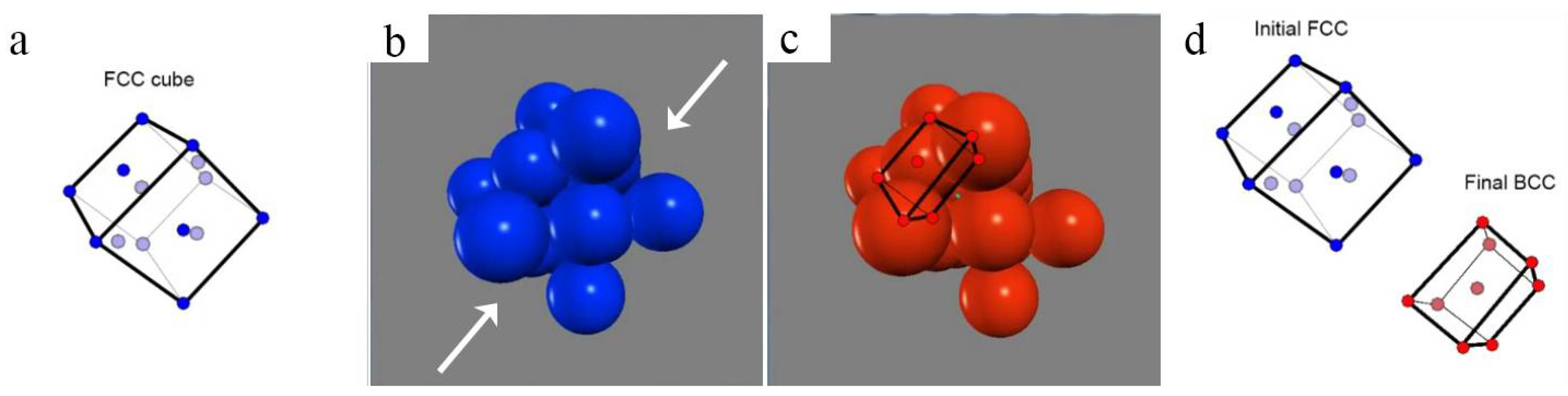
A one-step continuous model of the fcc-bcc lattice distortion leading to a KS OR was built similar to the one made with the Pitsch OR in [114]. This model also uses the hard-sphere assumption to explicitly calculate the trajectories of the atoms during the transformation, i.e., to obtain a continuous atomistic model of the fcc-bcc transformation [117]. The main idea can be briefly explained as follows. During the Bain distortion the fcc lattice is contracted along a <100>γ direction; the two other <100> directions are expanded; when the transformation is complete, half a bcc crystal is formed, as shown in Figure 20.
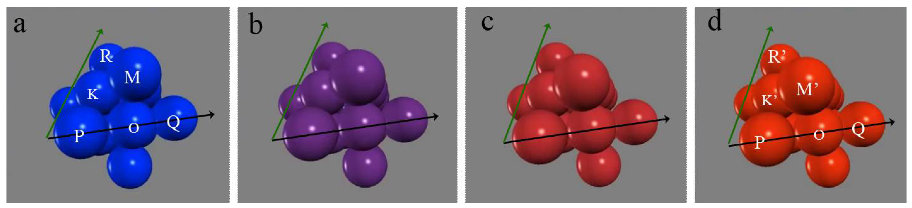
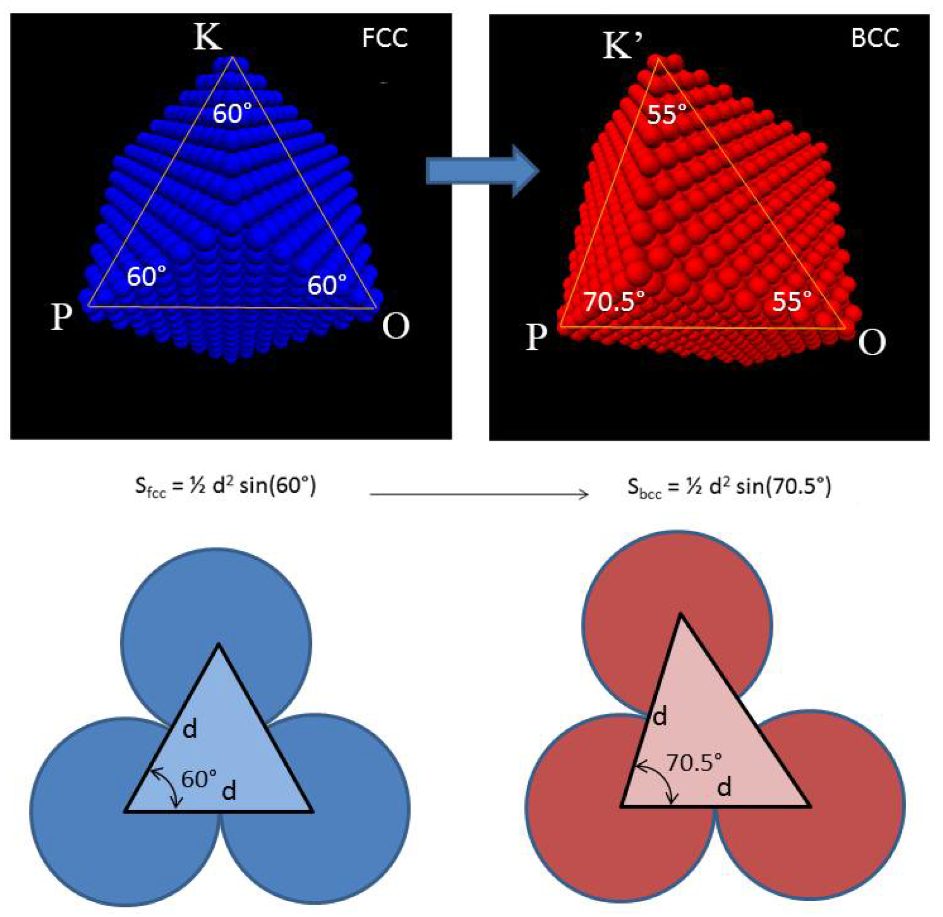
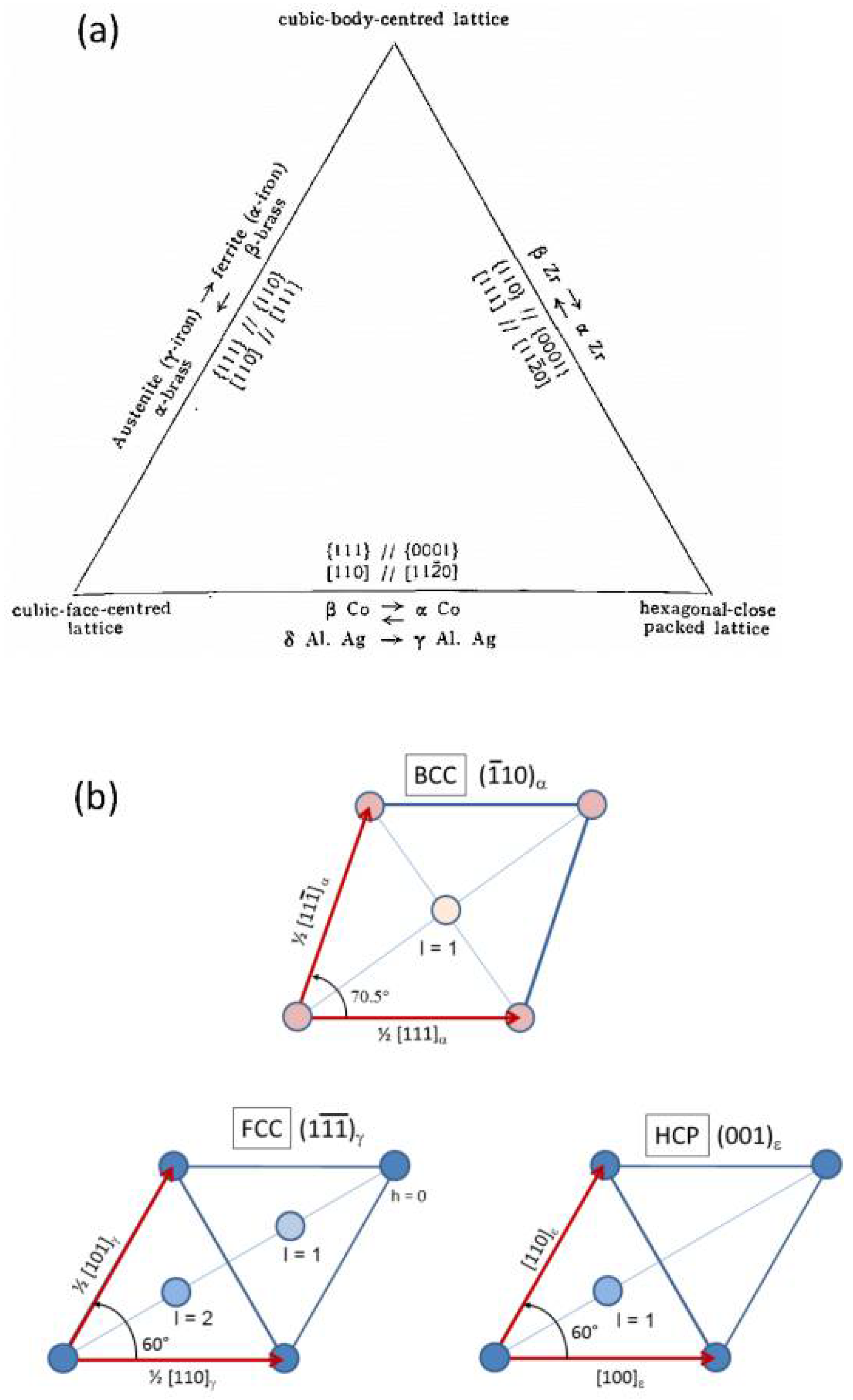
For the distortion that leads to the KS OR, simply called KS distortion, the trajectories of the atoms are slightly different from those obtained with the Bain OR. Let us consider Figure 21. The KS OR implies the parallelisms of a dense plane (POK) = {111}γ//{110}α and a dense direction PO = ½ <110>γ = ½ <111>α. The KS distortion is thus obtained as follows. The atom P is fixed. The angle β made by the dense directions (PO, PK) opens from 60° to 70.5° while maintaining the direction PO invariant; the atoms O and K lose contact, and the atom M in the upper layer, located above O and K, moves (“rolls”) over them to get closer to the atom P. When the transformation is complete, half a bcc crystal is formed (for Bain distortion), but now directly in KS OR.
For the KS OR expressed by (11)γ//(10)α & [110]γ = [111]α, the continuous form of the distortion matrix is
where x = cos(β). It can be checked that this distortion matrix is the identity matrix for the starting state β = 60° (X = 1/2); when the transformation is complete, β = 70.5° (X = 1/3), it becomes:
If one prefers using the equivalent KS OR, defined by (111)γ//(110)α & [10]γ = [11]α, the matrix of complete distortion is obtained by a change of reference frame
Even if the trajectories of the atoms are different, the calculations prove that the KS distortion matrix DKS is linked to the Bain distortion B by a polar decomposition DKS = RB. All the calculations used here are analytical; they result from simple geometrical considerations, and not from density functional theory (DTF) or molecular dynamics (MD). MD simulations help one understand displacive transformations, but one can doubt the capacity of brute force MD to simulate the coordinated “wave-like” displacements of atoms, even if it was proved that the phonon dispersion curves can be obtained by MD simulations [118]. Simulating a “phase transition wave” seems more complex than an acoustic wave, and it is probable that a better understanding of the transformations is required to add new crystallographic constrains to MD. The first MD simulations proposed by different groups in the last decade are going in the right direction [119,120,121,122]. For example, in 2008 Sinclair and Hoagland could simulate by MD the formation of bcc martensite in Pitsch OR, at the intersection of stacking faults [119]. Sandoval et al. showed in 2009 [120] that a pure Bain path would necessitate compressive stresses five times higher than with an NW path (see KSN model described earlier). Wang et al. could reproduce in 2014 the effects of the carbon content and cooling rates on the martensite start (Ms) temperature [121]. It is certain that MD will be an indispensable tool in the future to compare the “realisms” of the different crystallographic models, so efforts will be made in the future to combine the angular distortion with MD simulations.
The PTMC has the habit planes of martensite for output, but as already discussed, it makes post-dictions, not pre-dictions. Can a simple criterion be introduced to explain only the habit planes from the unique value of the distortion matrix? As there is no common plane between the fcc and bcc structures (even if this has never been formally proven), the IPS condition cannot be used. The PTMC made the choice to use it anyway, by combining it with other shears. The other possibility is finding a condition that is less restrictive than IPS. A criterion in which the habit plane is only untilted is physically relevant, because it avoids accumulating defects on long distances. The habit plane should be an eigenvector of the distortion matrix calculated in the reciprocal space, i.e., of the inverse of the transpose of DKS. The two only untilted planes determined with the matrix (15) are (111)γ and ; the latter plane is only at 0.5° away from the expected (225)γ habit plane. The calculation is direct, without any fitting parameter, and without knowing the details of the accommodation mechanisms in this plane. While writing the paper, [117], we realized that Jaswon and Wheeler [32] had already postdicted the (225)γ habit planes by calculating the distortion matrix related to KS OR, and by using an “untilted plane” criterion; therefore, it is true that part of our work [117] is actually an independent rediscovery of Jaswon and Wheeler’s. One should keep in mind, however, that Jaswon and Wheeler’s study is indeed rarely cited, and when it is, it is for the use of the Bain correspondence matrix and for introducing matrix algebra, not for the calculation of the KS distortion or for the “unrotated plane” criterion. As explained previously, Bowles and Barrett discarded Jaswon and Wheeler’s model very early in 1951 [48], that is why it is rarely mentioned in books on the PTMC; for example, it is not cited by Bhadeshia in his excellent and didactic book on martensitic transformations [38]. Bowles, Dunne, and many other metallurgists did not try to come back to Jaswon and Wheeler’s model, despite the huge difficulties they encountered in explaining the (225)γ habit planes, as recalled by Dunne [46]: “In contrast [to Mackenzie] John Bowles retained his intense concentration on martensite crystallography until he retired from the University of New South Wales in 1983. Bowles’ focus, moreover, was predominantly on the seemingly intractable {225}F problem and six of his nine PhD students works on aspects of this problem: Peter McDougall, Allan Morton, Druce Dunne, Don Dautovich, Peter Krauklis and Barry Muddle”. Recently, an anonymous reviewer claimed that the model of the KS distortion proposed in [117] was an “outright copy of Jaswon and Wheeler’s 1948 approach”. This is unfair if one considers the way we followed to come to the result, and if one compares the papers. Experienced scientists like to repeat Satayana’s aphorism “Those who cannot remember the past are condemned to repeat it”, but practically, how is it possible to remember or even know more than 5000 papers devoted to martensitic transformations in steels? More importantly, rediscovering also allows for exploring new directions. Only the matrix of a complete transformation was given by Jaswon and Wheeler, whereas the continuous KS distortion and analytical expression of the paths of the atoms could be calculated in [117].
Now, if one compares the model of [117] with the PTMC, the former gives directly and continuously the correct bcc structure, without adjusting parameters and without choosing additional shears, whereas the latter gives only the final structure and needs other parameters, such as the lattice parameters and a choice of LIS systems. All the steps of the transformation are now given analytically by a unique continuous parameter: the angle β made by the dense directions (PO, PK). This angle is the natural order parameter that is usually so difficult to define for first-order transitions. The distortion matrix has singular properties. Contrary to the Bain and Pitsch distortion matrices, it is not diagonalizable, and it has only two eigenvalues: 1 and 1.088 (which is the volume change due to the hard-sphere assumption). The eigenvector associated with unity is the parallel dense direction PO, and the eigenvector associated with 1.088 is a direction that lies in the untilted dense plane (POK), which means that contrary to an IPS, where the volume changes occurs perpendicularly to the invariant plane, here the volume change occurs inside the untilted (but distorted) plane. We will come back later to this property. This result is new, and implies that martensitic transformations should not be considered as a shear transformation. The notion of angular distortive transformation was thus introduced in order to replace the notion of shear.
With a large step back, the hard-sphere displacive model of fcc-bcc transformation appears as a convergent model of nearly all the models reported in the past. It substitutes a one-step angular distortion for the two shears of the 1930–34 KSN model, or for the two-step fcc-hcp → hcp-bcc model [110]; it is a continuous version of the underestimated 1948 Jaswon and Wheeler model of the KS distortion [32], and it replaces the four matrices of the 1952–53 PTMC models [33,34] by only one matrix. The model uses hard spheres as in the 1969 Bogers and Burgers model [53], but now it opens the correct angle on the correct dense plane. Indeed, in the Bogers and Burgers model shown in Figure 6, it is the angle between the untilted (111) dense plane (noted VQP) and another {111} plane (noted VSP) that was changed. The 60° angle between the dense directions in the plane VQP is not modified, i.e., the plane VQP is fully invariant before the second shear that allows the forming of the bcc structure. In the model shown in Figure 21, the untilted (111) plane is noted POK, and it is the angle between two of the three the dense directions of this plane (PO and PK) that is changed to directly obtain the bcc structure. In our model, there is no need for complementary shears as those proposed by Olson and Cohen in 1972–76 [56,57]. In addition, the important suspected crystallographic similarity with deformation twinning can be detailed and quantified. For example, fcc-bcc martensitic transformation and fcc-fcc deformation twinning can be geometrically represented in Figure 22, and quantitatively compared [123].
They shows that twinning results from a simple atomic displacement on each {111}γ layer, as in the usual representation, but the continuous atomic trajectories do not follow a simple shear strain because the atom M must go over the atoms O and K (and the angle β remains locked at 60°). This trajectory is familiar to any student in metallurgy who has already used ball stacking in ABCABC sequences in practical classes. The fcc-bcc transformation results from the same atomic displacements, except that now the movement of the atom M is combined with an increase of the distance between the atoms O and K (the angle β is unlocked and changes from 60° to 70.5°), which explains why the “jump” h of the atom M (the distance between the atom M and its projection on the POK plane) is lower than for twinning. For fcc-fcc deformation twinning, as the surface of the plane POK is constant, the change of the distance h implies a volume change during the distortion, even if, when twinning is complete, the volume comes back to its initial value. This result is actually expected from a hard-sphere model, because for fcc-fcc twinning the intermediate states are necessarily less dense than fcc (Kepler–Hales theorem). The curve of Figure 22b shows that the distance h also changes during the fcc-bcc distortion. When the distortion is complete, this distance comes back to its initial value, as it does for fcc-fcc twinning, despite the fact the bcc phase has a volume higher than for the fcc phase. The volume change between the initial and final states is completely due to the change of the surface of the plane POK ⟶ POK’ because of the angular distortion in which β = (PO, PK) increases from 60° to 70.5°, as shown in Figure 23.
In addition, it is qualitatively understood that the two components of the KS distortion, one given by the rotation of the direction PK around the normal to the dense plane POK, and the other by the tilt of the plane POM around the direction OK, produce the continuous rotations A and B observed in the pole figures Figure 19a. In this approach, the special arrangements of dislocations are generated by the rotational parts of the distortion: they form the disclinations at the origin of the rotations A and B, retained in the material as plastic traces of the mechanism. We are presently working to quantitatively simulate the continuous special features in the pole figures only from the analytical expressions of the distortion.
Even if, in first approximation, the mechanism of the fcc-bcc transformation can be modelled without knowing the exact nature of the accommodation processes, one can ask whether or not the “untilted plane” condition can be transformed into an IPS condition. The PTMC often changes the lattice distortion RB into an IPS by using an LIS on a (112)α plane, explaining that it corresponds to a mechanical twinning of the bcc phase, and forgetting that bcc metals generally twin only at very low temperatures (far below the usual Ms temperatures). The hypothesis made in [114] is that the “mechanical twins” are in fact KS twin-related variants. We discovered that the “untilted” (225)γ plane could be transformed into an IPS by combining two twin-related KS variants [124] misoriented by 60° around the common dense direction PO = <110>γ//<111>α. A movie of the continuous formation of a (225) martensite composed of two KS variants could be simulated (Figure 24).
These simulations are good agreement with the TEM observations of the midrib structure observed in the center of lenticular martensite products [125,126]. However, one should keep in mind that far from the midrib, martensite is only constituted of one variant, which means that during martensite growth the transformation obeys an angular distortion accommodated by dislocations, and no longer an IPS.
A model of the {557}γ martensite in low-carbon steels was also established [127]. The natural transformation is still the KS distortion for the {225}γ martensite in high-carbon steels, but the average is now made between the two low-misorientated variants that share the same dense plane; these two variants form an assembly called a “block”. The average distortion is exactly the distortion associated with the NW OR, and an eigenvector of the NW distortion matrix expressed in the reciprocal space (i.e., an untilted plane) is the plane, which is only 0.3° far away from the expected (557) plane.
7.5. Habit Plane and Surface Relief
Assume that the habit plane is an invariant shear plane at a mesoscopic scale (made of the martensite product associated with twins, twin-related variants, or periodic arrangements of dislocations) is the classical paradigm of PTMC. We have seen that Bowles and Barrett in 1952 [48] discarded Jaswon and Wheeler’s model of (225) martensite because of this paradigm. Two years later, Bowles and Mackenzie [34] detailed the reasons for which, according to them, the habit plane should be invariant. First, they stated that, “the amount of plastic deformation would be [unreasonable] extensive even for small rotations of the habit plane […] It can therefore be concluded that the habit plane is not rotated” (as also assumed by Jaswon and Wheeler). Then, they stated that “no line in the [habit] plane can be rotated […] A direct test of the accuracy of this conclusion is furnished by the observation that a martensite plate and the neighbouring matrix can kept in focus under a microscope while traversing the whole length of plate.” This sentence is essential because it is used to affirm that the habit plane, in addition to being untilted, is also undistorted, i.e., fully invariant. Unfortunately, the argument is not clear, and we do not understand why compatibility between the martensite and its parent austenite necessarily implies that the interface plane is undistorted. Peet and Bhadeshia [128] could observe, by atomic force microscopy, the surface relief produced by the formation of bainite at 200 °C. The surface, shown in Figure 25a, is interpreted by these authors as the resultant of a homogeneous shear (Figure 25b). It is in agreement with Bowles and Mackenzie; however, such a relief can be explained as well by an angular distortion, as illustrated in Figure 25c,d.
It is probable that, in many cases, mainly for the initial stages and for the midrib formation, the habit plane is rendered invariant by the co-formation of a pair of variants (as in Figure 24); however, that condition does not seem to be necessary for the growth of individual martensite, and cannot be used as a fundamental part of a mechanistic theory of martensitic transformation.
In brief, discarding the assumption of shear permitted the establishment of simple and coherent models of the {225}γ and {557}γ martensite, which is encouraging if one considers the very long history and the high number of publications on this subject. Besides, it was stated from the first quantitative metallographies that the habit planes of martensite are irrational, even if noted with high index rational numbers. Irrational values can now be proposed: according to our model the {225}γ observed in high-carbon steels and the {557}γ habit planes in low-carbon steels are {11γ and {11γ planes, respectively. The former are fully accommodated by coupling the twin-related variants that share the same dense direction, and the latter both by coupling the low-misoriented variants that share the same dense plane and by additional dislocations. The difference between these two modes might come from the difference of Ms temperatures; in the former case, the low Ms temperatures do not allow dislocation plasticity, but promote variant-pairing IPS accommodation, whereas in the latter case, dislocation plasticity allows for conditions that are less restrictive than pure IPS.
8. Generalization of the Angular Distortive Model to Face-Centered Cubic–Body-Centered Cubic–Hexagonal Close-Packed Martensitic Transformations, and to Face-Centered Cubic–Face-Centered Cubic Deformation Twinning
The hard-sphere model allows description with the same formalism the mechanisms of both deformation twinning and martensite transformation. The model permits a natural introduction of an order parameter into the transition; the order parameter is simply the angle of distortion (and not an ill-defined multidimensional strain state). The work done for the fcc-bcc transformation was thus quickly generalized to other displacive transformations between the fcc, bcc, and hcp phases observed in other metal alloys [123]. By noting that fcc = γ, bcc = α, and hcp = ε, as it is usually done for steels, the classical ORs between the three phases are the KS OR for fcc ⟶ bcc, the Burgers OR [29] for bcc ⟶ hcp, and Shoji-Nishiyama (SN) [37] for fcc ⟶ hcp transformations:
These respect the parallelism of the close-packed directions, and form a close set of ORs that is of interest to build a unifying theory, as already noticed by Burgers in 1934 and illustrated in Figure 26a. The three phases projected along the normal to their common dense plane is shown in Figure 26b. The use of angular distortion matrices offers the possibility of treating these transformations similarly in a unique framework, with the same paradigm. The fcc ⟶ hcp and bcc ⟶ hcp transformations involve shuffling, because the parent and daughter phases do not have the same number of atoms in their Bravais cell (the bcc and fcc primitive cells contain one atom, whereas the hcp primitive cell contains two atoms). The distortion matrices and shuffle trajectories (when required for the hcp phase) were analytically determined as functions of an angular parameter that depends on the transformation. The choice of an angular parameter and the details of the calculations are given in [123]. It is important to note that both the lattice distortion and shuffling are the two sides of the same coin; there is no reason to disconnect them.
Some movies showing the atomic displacements were simulated, with some snapshots shown in Figure 27. They illustrate the atomic displacements during the transformation process by using an initial single crystal with a cubic shape. The exact morphology of the martensite product and the details of the accommodation mechanisms were not yet considered in these simulations.
The habit planes are calculated according to the “untilted plane” criterion. For bcc-fcc transformations and for bcc-hcp transformations, they are and , respectively. They are less than 15° away from the habit planes reported in literature. This agreement is thus quite good, if one considers that there is no free parameter at all in the theory. Of course, the interface plane of the martensite in these alloys is more complex, in that a simply untilted plane, along with the dislocations, twins, and twin-related variants that structure the martensite interface are not taken into account by the model for the moment, except for the (225) martensite (Figure 24). In the same spirit, one-step crystallographic models of martensitic transformation using the hard-sphere assumption were proposed recently by Sowa [129]; the main difference with our approach is that the models are based on group-subgroup chains of intermediate structures.
9. Angular Distortive Model for Deformation Twinning in Hexagonal Close-Packed Metals
9.1. Application to Extension Twinning
The cases of deformation twinning in bcc and hcp metals were not investigated in [123], because they are more complex than for fcc-fcc twinning. The investigations on deformation twinning in magnesium were only started three years ago. Among hcp metals, magnesium was chosen because the ratio ≈ 1.625, which is close to the ideal hard-sphere packing value of ≈ 1.633. For extension twinning, the displacements of the Mg atoms were quite easy to determine [130]. A brief explanation is given here. The twin–parent misorientation is a rotation of 86° around the common a-axis. Instead of working directly with this misorientation, it is simpler working on a “prototype” Bain-like stretch twin with a 90° misorientation, and do the first calculations in the orthogonal basis xyz shown in Figure 28a. The lattice stretch results from an exchange between the basal and prismatic planes, as shown in Figure 28b. This exchange can be visualized by considering the XYZ supercell containing four atoms, and is a consequence of a simultaneous rotation of angle η of the three atoms inside the cell. The lattice stretch induces a slight rotation of the plane, called obliquity. The obliquity angle ξ shown in Figure 28c can now be calculated and continuously compensated for, in order to leave the plane untilted during the twinning distortion, such that the final twin–parent misorientation is (86°, a). The analytical equations of trajectories of all the magnesium atoms are established as functions of a unique angular parameter (as for martensitic transformations). It was shown that the habit plane is not fully invariant during the twinning process; it is just untilted, and restored when the distortion is complete. Indeed, the distance OV in this plane is not constant (Figure 28d). In addition, there is a volume change of 3% during the distortion (Figure 28e), as expected from Kepler–Hales’ theorem for a transition between two hcp states. This volume change cannot be totally accommodated elastically, which means that plasticity is required to accommodate the twinning distortion in polycrystalline alloys.
This work conciliates inside a unique model the (90°, a) twins observed in nano-pillars [131] and the (86°, a) usual twins observed in bulk samples. Both twins result from the same atomic displacements and lattice distortion, and differ only by their obliquity. At this step, the model does not imply imagining twinning dislocations, disconnections, or any complex mechanism involving dislocations. Some elastic strains are induced, and some dislocations are emitted by the distortion, and that could be interesting to determine how they can be predicted from the distortion matrix and from the usual slip systems in magnesium, but that is beyond the model in its current form.
As the distortion is not a simple shear, a new criterion had to be introduced to substitute Schmid’s law. It is often reported that twins can form in hcp metals despite low or even negative Schmid factors [132,133,134,135]. This “non-Schmid” behavior is usually explained by invocating that the local stress fields in the grains differ from the applied stresses, but another explanation is worth being considered. The intermediate state, at the maximum volume change, implies the largest strains perpendicularly to the habit plane; therefore, it is conceivable that this state constitutes an energetic gap for the twin formation. Twinning occurs when the work performed by the external stresses accompanying the twin formation is higher than this energetic gap, or is at least positive. The general formula of the work W done during a lattice distortion where D is the distortion matrix and I the identity matrix occurring in a fixed stress field is
Whereas the usual shear model with Schmid’s law predicts the formation of extension twins during uniaxial tensile tests with parent crystals tilted in the range , as shown in Figure 29a, the hard-sphere displacive model associated with the work criterion predicts a range of , as shown in Figure 29b. Experimental studies would be needed to confirm this prediction. It should be noted that for fcc-fcc deformation twinning, the difference between Schmid’s law and the work criterion at maximum volume change is hardly perceptible, as shown by Figure 29d–f (unpublished result); which could explain why non-Schmid behavior of the mechanically twins in fcc metals has never been observed.
9.2. Comparison with the Pure-Shuffle Model
Another model of extension twinning without twinning dislocations exists in literature. In 2009, Li and Ma “observed” the results of MD simulations and proposed an “atomic shuffling dominated mechanism” [136]. In 2013, Wang et al. also noticed in the MD simulations a nucleation step obeying a “pure shuffle mechanism”, the growth being accomplished “via the conventional glide-shuffle mechanism” [137]. These authors also used the expressions “unit cell reconstruction” [138], and “twinning with zero twinning shear” [139], which can make one think that the mechanism is diffusive across short distances. Li and colleagues define shuffling as “inhomogeneous displacements of an ensemble of atoms in the layers immediately adjacent to the TB [twin boundary]” [136], and twinning growth is imagined as a boundary migration where “the TBs can migrate freely and fully consume the parent grains” [139]. This definition can be quite confusing. Shuffling is historically invocated when some atoms in the unit cell do not follow the same trajectories as those located at the nodes of the lattice. As written by Christian et al., “a shuffle only rearranges the atom positions within a unit cell” [140]. For example, as the hcp unit cell contains two atoms, the martensitic transformations between fcc and hcp, or between bcc and hcp, require an additional shuffling of half of the atoms, as shown previously in Figure 26. The shuffling equations are analytically determined for these transformations in [123]. Transformations between a simple phase with a small unit cell, and a complex phase with a large unit cell containing a high number of atoms, imply large and complex shuffles, as it happens in many shape memory alloys—for example, the B2 ⟶ B19’ transformation in NiTi alloys [141].
It is not surprising that shuffling and distortion are correlated in metals, as experimentally found by Wang et al. for the bcc-hcp transformation in titanium [142], because the lattice distortion and the displacement of the atoms in the lattice are intrinsically correlated. Similarly, deformation twinning in hcp crystals imagined as an hcp-hcp transformation involves shuffling. In the example of extension twinning in magnesium, a quarter of the atoms (those at the nodes of the XYZ lattice) follow the trajectories given by the distortion matrix, and three quarters of the atoms shuffle inside their local XYZ cell. Consequently, in its traditional meaning, shuffling cannot exist for itself; if it exists, it is always concomitant with a lattice distortion. In Christian et al.’s words: “shuffles can only be avoided if both structures have primitive unit cells containing only one atom” [140]. This meaning has digressed over time, with the introduction of the concept of “shuffle transformations”. Christian et al. define them as follows: “A pure shuffle transformation requires that some unit cell of one lattice is almost identical with a cell of the other lattice” [140]. Delanay uses a more precise definition: “A shuffle is a coordinated movement of atoms that produces, in itself, no lattice distortive deformations but alters only the symmetry or structure of the crystal; a sphere before the transformation remains the same sphere after the transformation” [143]. He adds later: “Shuffle transformations are not necessarily pure; small distortive deformations may additionally occur. They therefore also include those transformations involving dilatational displacements, in addition to the pure shuffle displacements, provided that they are small enough not to alter significantly the kinetics and morphology of the transformation” [143]. Therefore, a pure shuffle transformation is a transformation that should not significantly change the lattice; this is not the case for extension twinning, and that is why the idea of “pure shuffle” is unclear. It is difficult to imagine that the atoms can move independently of the lattice in which they are contained. This would be possible with a big lattice containing many, largely-spaced atoms of small size, but is completely impossible with a hard-sphere model, in which the atoms are in contact, as proved by the calculations of [130]. When the atoms move, the lattice is distorted, and vice versa. There is no possibility of elastically accommodating atomic displacement in the unit cell while maintaining the unit cell dimension. Liu et al. are more cautious than Li and Zhang in their use of vocabulary; they clearly specify that “UCR [unit cell reconstruction] produces tetragonal deformation instead of simple shear” [138]. It should be interesting to clarify the role of the external stresses in the “pure shuffle” model. Despite the possible confusion raised by the term “shuffle”, we can notice that this model is probably not so different from the hard-sphere model we propose. Indeed, the trajectories of the atoms shown in Figure 3 of [137] and reported in Figure 30a seem to be the same as those shown in Figure 28a. The trajectories reported in Figure 4 of [131], shown in Figure 30b, are different, but the rotation and mirror symmetries between the figures makes an exact comparison difficult. The conclusions reached by both models are also convergent: “the {10–12} twinning plane cannot remain invariant during twinning” and a mechanism “without the need of twinning dislocations” is possible [139]. It is also interesting to note the very good agreement between the DTF calculations made by Ishii et al. [144] and the analytical calculations presented in Section 9.1. For example, the energy landscape given by DFT presents an energy barrier due to shuffling, as if “something internal ‘got stuck’” [144], and this barrier was found at the midway point of the transformation process, as with the maximum volume change calculated analytically (Figure 28e). The DTF results can thus be interpreted by the fact that the atoms in the unit cell get too close to each other (the spheres interpenetrated one another) when a simple shear is applied, i.e., when no dilatation perpendicular to the twin plane is allowed. This type of strain does not let the cell “breath” and reach the volume change required by the intermediate state (+3%). If the analytical approach permits obtaining a qualitative understanding of the mechanism, DFT remains necessary to quantify the energies and compare them with the experiments.
We believe that the coupling between shuffling and lattice distortion observed in the extension twins is a general phenomenon, and we do not think that “[the extension twinning] mechanism distinctively differs from any other twinning modes” [139]. We have shown that deformation twinning can be modelled by a distortive mechanism, in which all atoms can move collectively at the speed of sound, or at lower speeds if time is needed to reorganize the dislocations emitted by the distortion and relax the back-stresses in the surrounding matrix. Therefore, to our point of view, the mechanism of extension twinning in magnesium does not differ from the other deformation twinning modes. All the modes should imply an angular distortion, and many of them (but not all of them) become a simple shear when the distortion is complete.
The advantages of the distortive model of deformation twinning is that it can be combined with mechanical calculations, such as Equation (17) in order to explain why twins are formed and for which orientations they are formed. Contrary to the shuffle model, the distortive model makes macroscopic predictions. On the other hand, it is true that the distortive model does not yet explain the microscopic characteristics at the twin interface, such as the fact that the interface plane is often not straight but made of basal-prismatic segments. Partisans of “pure-shuffle” insist on these features as if they were a specific property of extension twinning, but the existence of a segmented interface is a quite general property of displacive transformations. The formation of terraces and ledges are observed for the deformation twins in the Twin Induced Plasticity (TWIP) steels, and for many diffusive and displacive transformations, as proved by the HRTEM observations made by Ogawa and Kajiwara in martensitic iron alloys [145]. At a mesoscale, the lenticular shape of extension twins in magnesium can also be observed for other deformation twin modes and in other metals and alloys, as in TWIP steels (Figure 31b). Thus, neither the basal-prismatic segments nor the lenticular shape are proof of a pure-shuffle mechanism; they can be formed displacively as well.
In brief, it seems that the “pure-shuffle” and the “distortive” visions could be mixed, because they are not antagonistic. Both approaches have strong arguments [146]; they agree to say that the dislocation twinning and the complexity of the topological model are actually unnecessary to explain the twinning mechanism. In addition, both discard the classical assumption that extension twinning is a simple shear mechanism. However, Li and Ma think that the non-shear character is limited to the {102} twinning mechanism, and that “this should not be deemed as the failure of the classical theory”, whereas we believe that there is nothing special in the mechanism of extension twinning in magnesium, and that all the deformation twinning modes and all the martensitic transformations obey the same crystallographic rules. The angular distortive paradigm proposes a way to get this unification.
9.3. Application of the Distortive Model to Other Twinning Modes
There is another important difference between the pure-shuffle and the distortive approaches. The former relies on MD computer simulations to explore new twinning modes, and extract some hints and rules to build crystallographic models, whereas in the latter, the computer is just used to help the analytical calculations that, at least in theory, could be done by hand. The displacive model is purely geometric; this simplicity is a force to understand and explain the various twinning modes in metals. For example, the hard-sphere displacive model was also recently applied to {101} contraction twinning in hcp metals [147], as shown in Figure 32, leading to similar conclusions, i.e., the volume of the unit cell was not constant and the habit plane was not invariant during the process; it was just untilted and restored when the process was complete, and the distortion matrix then became a simple shear matrix. The result was a shear of amplitude s = 0.358 on the plane (01) along the axis [18, , ], which was not predicted by Bevis and Crocker’s theory. It was recently realized, by writing the shear direction with four indices, i.e., −[, 28, 13, 5], that this shear mode is exactly the same as that given by Serra et al. in their list of three possible {101} twinning systems given in Table 1 of [148], calculated from the translation vectors between the parent and twin crystals (i.e., vectors of the dichromatic structure) [149]. This confirms the validity of the calculations [147], and also proves that an approach different from a disconnection model is possible.
There is no technical obstacle to apply the same approach to other twinning modes in magnesium, or to bcc-bcc twinning modes, and a general theory of deformation twinning compatible with a hard-sphere assumption can be developed in the near future.
It is important to note that the habit plane is not an invariant plane, but just a plane restored from the intermediate state when the transformation is complete. The possibility that the plane is transformed into a new plane different from the initial one is offered by the new paradigm. We recently found, by EBSD, a new and unconventional twin in a magnesium single crystal [150] that is incompatible with simple shear but corresponds exactly to this case. This twin is a cousin of the usual (112) and (112) twins; actually, the three twins derive from the same prototype “Bain” stretch detailed in [151], and differ only by their obliquity correction.
9.4. Comparison with Earlier Atomistic Models of Hexagonal Close-Packed Twinning
In 1980, Dubertret and Le Lann proposed models of twinning in hcp metals [152,153] that were cited by Wang et al. [137] as references for the concept of shuffling. These models were nearly forgotten, despite or because of the huge amount of literature on deformation twinning. They are also based on hard-spheres, but a direct comparison with our models is difficult because the atomic displacements are expressed from tetrahedrons associated with the odd condition where . The main initial idea is the same as that used in the pure-shuffle model, and the c/a ratio was probably chosen to let the atoms move and exchange their positions in the lattice, without changing the lattice dimensions in order to be in a pure-shuffle case. Despite this choice, and the absence of correlation between the atomic displacements and the lattice distortion, Dubertret and Le Lann clearly understood that {102} extension twinning and {101} contraction twinning are obtained by atomic displacement that produces a crystallographic exchange (correspondence) between the basal and a prismatic planes in the former case, and between the basal plane and a {101} plane in the latter case. They called these exchanged planes the “corrugated planes”. Going deeper into historical considerations, it is interesting to note that the initial 1968 Kronberg model [154] on which Dubertret and Le Lann’s works are based also uses a hard-sphere representation of the atoms, and creates a correlation between the atomic trajectories and the lattice distortion, as shown in Figure 33.
10. Future Works and Perspectives
10.1. The Distortion Angle As a Natural Order Parameter
Thermodynamic models of phase transitions are based on a parameter called the “order parameter”. In phase field models (see for example [155,156]), the order parameter is simply the proportion of phases, i.e., a real number between 0 (parent phase) and 1 (daughter phase), with the interface encoded by a real value between 0 and 1. Some models try to find a physical parameter that controls the order parameter, but the choice depends on the type of transition. It is usual to differentiate second-order and first-order phase transitions (note that the meaning of term “order” is different from that of “order parameter”). Second-order transitions imply small atomic displacements, so that the parent and daughter phases are very close. The daughter phase is formed directly from the totality of the parent phase without coexistence of the two phases. First-order transitions imply large displacements of atoms and an important lattice distortion; in addition, the transition is accompanied by a latent heat. The energy required to accommodate the daughter phase inside the parent phase is such that the two phases generally coexist, and an important undercooling is required to reach the complete transformation. The order parameter that defines the daughter phase continuously changes from 0 to 1 in second-order transitions, and is abruptly and discontinuously modified from 0 to a non-null value in first-order transitions. The distinction between second- and first-order transitions is quite arbitrary. All the structural transitions imply an accommodation process in the surrounding matrix, and thus a dissipation of energy. Of course, if the distortion is small, as in the “displacive” transitions (with the physical meaning, i.e., small atomic displacements), the accommodation is mainly elastic, the transition is reversible, and the hysteresis is small; whereas if the transition is “reconstructive” (with the physical meaning, i.e., breaking of the atomic bounds and formation of new ones), the distortion is large and implies plasticity. It is often assumed that the former are second-order and the latter are first-order, but the distinction is more quantitative than qualitative. It is also usual to assume that when a group–subgroup relation exists, the transition is second-order, and when this relation does not exist, the transition is first order; however, one can imagine a cubic-tetragonal distortion with very high distortion amplitudes that would be irreversible (and thus would be of the first order). Mnyukh [157] came to the extreme conclusion that the distinction between the first and second order transitions is artificial, and that all the transitions are first-order, only differing by the amplitude of the discontinuity.
Second-order transitions are generally modelled by the Landau theory [158]. The order parameter is arbitrarily chosen depending on the physical property that is judged of interest; it can be the variation of the local density for liquid-crystal transitions, as in Landau’s paper [158], the atomic displacement or polarization for ferroelectrics, the variation of the probability of site occupancy for order–disorder transitions, etc. The free energy is expressed by a Taylor decomposition into a polynomial form of the order parameter, and the polynomial coefficients depend on the temperature and pressure. The order parameter is the solution of the null derivative of this polynomial; it is zero at high temperature and non-null below the critical transition temperature Tc, and it continuously varies as a function of the temperature (Figure 34 a,b).
The Landau theory [158] is phenomenological because of the ad-hoc choices of the polynomial exponents and coefficients, but it gives an important mathematical framework for the use of symmetries in thermodynamics. Landau stated that the order parameter is a multidimensional parameter, which has as many degrees of freedom as the number of dimensions of the irreducible space chosen for the irreducible representation of the group of the parent phase. This concept is now didactically explained in many modern textbooks. In the example of cubic-tetragonal ferroelectric transitions, one irreducible space is the one-dimensional space z (the direction that will becomes the c-axis of the tetragonal phase), and the other irreducible space is the two-dimensional space (x, y). The use of the group representation’s theory in physics was quite natural, as it was already introduced few years earlier in fundamental physics, mainly by Wigner [159] and Weyl [160]. Group representation was and still is considered to be a major part of group theory; it has acquired important success in materials science, mainly in spectroscopy with the calculations of the Raman frequencies.
The martensitic transformations and deformation twinning are first-order structural transitions. It is agreed that the order parameter is a discontinuous function of temperature (Figure 34c,d). What is the order parameter for these transformations? Defining it is an old and difficult problem. Clapp, for example, wrote:
Different order parameters have been proposed beside the “volume fraction” mentioned by Clapp. For example, Flack [95], and more recently Clayton and Knap [162], proposed to use the shear strain(s). Beside the problem of defining the order parameter, Landau’s theory is based on the idea that the transition is a loss of symmetry, and thus cannot be applied directly to first-order transitions. Indeed, in metallurgy, many transformations are in between very distinct phases without group–subgroup relations, for example fcc-bcc transformations. Some symmetry elements are lost, but others are created. These transitions are also called in physics “reconstructive” (the meaning here is different from that used in metallurgy, where it is synonymous of “diffusive”). An interesting and powerful generalization of Landau’s theory of reconstructive transitions was proposed by Tolédano and Dmitriev [163]. The effective order parameter is a variation of a density function that is a sum of wave functions. The periodic form of this parameter permits one to decompose the free energy as a truncated Fourier series of the order parameter (and no longer a Taylor series). Many examples of applications from crystal to quasicrystals are studied and described in [163]. The density-wave description is an important element of generalization that establishes a first link with the wave propagation mode. However, the systematic use of a latent lattice, relevant for order–disorder transitions, would require more physical justifications for martensitic transformations. Besides, Tolédano and Dmitriev’s book [163] aims at physicists, but it does not use the classical vocabulary and concepts of metallurgy, and it does not respond to some basic questions raised by metallurgists—for example, about orientation relationships and the habit planes.Certainly one of the stumbling blocks in defining a martensitic transformation is that there is no obvious order parameter" associated with it, such as one has with ferromagnetic transformations (magnetic moment), order-disorder (long range order parameter), etc. Of course, one always has the possibility of using the volume fraction transformed as such an order parameter, analogous to the use of the fractional density of superconducting electrons for superconducting transformations, but this is a much more erratic quantity (markedly dependent on sample history) in the case of interest here.[161]
Important work on mutual understanding remains to be done, to build a real bridge between the developments made in physics and those made in metallurgy. The angular-distortive models presented in the previous sections show that a one-dimensional order parameter (simply the angle of distortion) can be chosen for many martensitic transformations and deformation twinning modes. This parameter is physical, controlling both the atomic trajectories and the lattice distortion. It is, however, not yet clear to us how this parameter could enter into the framework of Landau’s theory or into its advanced reconstructive version. Indeed, there is a fundamental difference in the way the symmetries are mathematically treated. Let us explain it with the simple questions: how many variants (domains) and how many types of domain boundaries are created by a phase transition? We were confronted to this problem when we had to find a method to reconstruct the prior parent grains from EBSD data (Figure 18). Instead of using the theory of group representation (based on the action of the group by conjugation), as in Landau’s and Tolédano and Dmitriev’s theories, the action (distortion) was treated by a left multiplication. The distinct orientations of the domains are called orientational variants. For some special parent/daughter orientation relationships, the parent and daughter phases have some symmetry operations in common; these symmetries form a subgroup of the point group of the parent phase, called an intersection group. The orientational variants are the left cosets based on this subgroup. More explicitly, we call Gγ and Gα the point groups of the parent and daughter phases, respectively; there is no need to imagine them as abstract groups that should be decomposed into irreducible representations. A point group here is simply the set of 3 × 3 matrices of symmetries tabulated in the International Tables for Crystallography. Let us also call the coordinate transformation matrix deduced from the orientation relationship. The symmetries of the daughter crystal, expressed in the parent basis, are given by the matrices Gα ()−1. The intersection group is thus Hγ = Gγ ⌒ Gα ()−1. The set Hγ is a subgroup of Gγ. The distinct orientational variants αi are defined by the left cosets Hγ, and their orientations relative to the parent basis are = with . One must understand “”, as a matrix arbitrarily chosen in the coset of matrices . By convention, is the identity matrix. The number of orientational variants Nα is the number of cosets on Hγ; it is the cardinal of Gγ/Hγ, and is given by the Lagrange formula: Nα = ∣Gγ∣/∣Hγ∣. More details are given in [105].
Now, we consider the different distortion matrices at the origin of the orientational variants. A distortional variant is defined by its effect on the initial shape of a crystal. An initial parent crystal of a shape whose symmetries form a group Gγ becomes, after complete distortion, , a daughter crystal whose shape has symmetries given by the matrices Gγ ()−1. The “distortional” intersection group is formed by symmetries that are common to the crystal before and after distortion, i.e., Kγ = Gγ ⌒ Gγ ()−1, with Kγ as a subgroup of Gγ. The distortional variants di are defined by the left cosets Kγ. The number of distortional variants Mα is the number of cosets on Kγ; it is the cardinal of Gγ/Kγ and is given by the Lagrange formula: Mα = ∣Gγ∣/∣Kγ∣. Generally, Kγ is a subgroup of Hγ, which means that the number of distortional variants is higher than the number of orientational variants: Mα ≥ Nα. More details are given in [123].
Let us come back to the orientational variants. The special misorientation between those variants, simply called operators, are defined by the double cosets Hγ\Gγ/Hγ. The number of operators is given by Burnside’s formula. In addition, the algebraic structure of the variants and their operators is a groupoid, and the groupoid composition table (imagined for the purpose) can be used as a crystallographic signature of the phase transition [105]. These ideas are not completely new; important results about coset and double-coset decompositions were already discovered by Janovec [164,165] in ferroelectrics, and the intersection group was found by Kalonji and Cahn for transitions without group–subgroup relation in their theoretical study of grain boundaries [166]. The mathematical notion of a groupoid unifies these notions and allows their generalization. A groupoid structure for the distortional variants, similar to that of the orientational variants, seems conceivable. Since the distortion matrices simply depend on a one-dimensional order parameter (the angle of distortion), these matrices, or their associated angular order parameter, could be used to build an Mα-dimensional space for the polynomial form of the free energy. In a broad way, one would replace the group representation theory used in Landau’s theory by a groupoid theory, based on cosets and double-cosets. One could hope that to find a polynomial form of the free energy whose solutions would constitute a groupoid. We recall that groupoids were initially introduced by Brandt in 1926 [167,168] for quadratic forms. The main idea here would be to find a groupoid on the set of solutions of the polynomial form of the free energy that would be an isomorph to the groupoid of distortional variants. One way to show the isomorphism could be to compare the composition tables of both groupoid structures. The idea is still vague, and such research would require the help of mathematicians.
10.2. Dynamics of Phase Transformation and Accommodation Phenomena
During a martensitic transformation, all the atoms move collectively; however, as previously discussed, this does not mean that all the atoms move together at the same time. Imagining that the transformation propagates in the material as a wave permits escaping Frenkel and Cottrell’s issue about the unrealistic critical stress required for an instantaneous and homogenous shear. It is indeed possible to use the continuous analytical form of the angular distortion matrix of a structural transformation D(β), where β is the distortion angle, to generate the martensite phase continuously but heterogeneously in space and time. One way could be to find an analytical equation for the order parameter β that depends both on the position r and the instant t. For example, let us introduce (i) the position of the parent interface L(t), which moves at a wave velocity c; and (ii) a length of accommodation (LA), without detailing for the moment whether the accommodation is elastic or plastic. An interesting form of the order parameter is given by a linear ramp function
where is the finished distortion angle, i.e., D() is the matrix of complete distortion, is the start distortion angle, i.e., D() = Identity, and L(t) = c.t. The regular letters r and L mean the norm of the vectors r and L. This ramp function is shown in Figure 35.
One can imagine that L(t) is a function of the position vector r; for example, the length of L(t) can be inversely proportional to the amplitude of strain at the position r, such that. , where , and ε is an additional constant added to avoid infinity issues. The model, applied to the 2D hexagon–square distortion presented in Figure 12, allows the simulation of simple dynamic and crystallographic atomistic movies; some snapshots are given in Figure 36. The movie shows a hexagonal lattice of hard-disk atoms constituting a round crystal, which is continuously and heterogeneously distorted to be transformed into a square lattice of hard disks forming an elliptic crystal at completion. The LA was chosen to be equal to the size of the crystal, in order to minimize the change of distance d between the neighboring atoms. Actually, the LA could be arbitrarily chosen such that d does not deviate from the initial interatomic distance (atom diameter) by more than a fixed and low value that agrees with elasticity. In addition, it seems possible to replace the linear ramp by a more complex form (for example, the one indicated by the dashed curve in Figure 35) that could minimize the maximum interatomic distance (di-d) on the set of the atoms i. This approach could be also investigated to check whether or not the existence of parallel dense directions and planes would favor the wave propagation, which could then be used to determine a new criterion to predict the “natural” parent–daughter OR. This also starts establishing a link with the Ginzburg–Landau theory [169], in which the gradient of the order parameter is taken into consideration in the analytical form of the free energy, here with the advantage of including the atoms, the lattices, and many crystallographic tools that are of interest for martensitic transformations (distortion, correspondence, and orientation).
11. Conclusions
The concept of simple shear has been the corner stone of the classical theories of the crystallography of martensitic transformations and deformation twinning for 150 years. The early models of the fcc-bcc transformations proposed by Young, Kurdjumov, Sachs, and Nishiyama, those of the bcc-hcp transformations made by Burgers, the phenomenological theory of martensitic transformations (PTMC) initiated by Greninger and Troiano and developed by Weschler, Read and Liebermann, and Bowles and Mackenzie, and lastly the theory of deformation twinning developed by Bilby, Bevis, and Crockers, among others, are all based on compositions of simple shears, or imply an invariant plane strain (IPS), which is a generalized form of shear that accounts for the volume change induced by the transformation. The mathematical treatment is irreproachable, although complex due to the initial premises. The predictive character of these theories is more limited than what is often claimed, which may explain why the theories have evolved over time by the addition of new shears (double- or triple-shear, double-shear versions of twinning), i.e., by adding new layers of complexity. An important problem of the shear paradigm was raised by Frenkel’s calculations (corrected later by Orowan and Cottrell); it shows that an instantaneous simple shear is impossible under realistic stresses, or without the help of dislocations. Cottrell [54] and Bilby [13], followed by Sleeswyk [69], Venables [73], and Christian [2], among others, thus came to imagine additional mechanisms by which the deformation twins are created by sequential and coordinated movements of partial dislocations, called “twinning dislocations”. Sleeswyk also proposed that the twinning dislocations dissociate into “emissary dislocations”, before moving away from the interface to reduce the stresses [69]. Often, TEM images of partial Shockley dislocations in front of twins or martensite are shown as a proof of the existence of “twinning dislocations”. The concept of a dislocation-mediated mechanism of twinning was generalized to displacive transformations by Hirth, Pond, and co-workers [84]; here, the twinning dislocations were replaced by “disconnections”, specifically designed to model the ledges at the parent–martensite interfaces. In this framework, the mechanism of the martensitic transformation is envisioned as the result of the interface displacement, and the martensite growth depends on the glissile character of the disconnections at the interface. Important questions are not addressed by these models. The pole mechanism and its derivatives do not convincingly explain how the dislocations/disconnections are created, and how they propagate in a sequential and coordinated way at speeds close to the acoustic velocities. In addition, the fundamental question of “how do the atoms move?” remains unsolved.
In order to respond to this question, in the case of transformation between fcc, bcc, and hcp phases in metals, the assumption was made that the atoms move as hard spheres. The concept of simple shear has thus to be replaced by that of angular distortion, because the volume change of the intermediate states is higher than that allowed by simple elasticity. The sole input data is the final orientation relationship between the parent and the twin/martensite daughter phases. There is no other free parameter. A unique one-dimensional angular parameter, specific to each transition, allows the analytical calculation of the trajectories of all the atoms. The lattice distortion and shuffling (when required) appear as both sides of the coin. Obviously, the distortion can be decomposed into infinitesimal combinations of stretches and rotations, or LIS and IPS, as in the PTMC, but this decomposition would be artificial and of low interest. In the framework of this new paradigm, it is not required that all the atoms move instantaneously; martensite may actually be formed as a “lattice distortion wave” that propagates at high velocity and around which an accommodation zone can be spread across large distances, in order to maintain the interatomic distances in the material below the elastic limit. It is conceivable that the accommodation is elastic in the first stages of nucleation and growth, and becomes plastic when the martensite size becomes comparable to the grain size. In this way, contrary to the usual dislocation/disconnection–mediated models, the dislocations are not the cause but appear as a consequence of the lattice distortion. The partial dislocations shown by TEM in front of the mechanical twins may be created and emitted by the twin/martensite itself, and not by hypothetical pole mechanisms. When the lattice transformation is achieved, the angular distortive paradigm allows finding the same results as in shear-based theories in some classical cases, as for the {225} martensite in high-carbon steels, the deformation twins in fcc metals, and the extension twins in hcp metals. The angular distortive paradigm is, however, more general than the shear one; it allows the calculation of the atomic trajectories, and also opens new possibilities. The habit planes can be determined with a criterion that is less restrictive than with the shear paradigm; it is assumed that the habit planes are those untilted by the distortion (they are not necessarily fully invariant). Different accommodation mechanisms are possible: variant pairing, special dislocation arrays that close the rotational gaps (disclinations), etc. In our opinion, these mechanisms can be studied in a second stage; there is no need to imply them directly in the mechanism of transformation, and no need to impose gliding conditions on the interface in order to understand the propagation of a martensitic transformation. Undercooling or external stresses are important to obtain sufficient chemical or mechanical energy, in order to create the elastic or plastic accommodation zone required by the lattice distortion. In athermal martensite, the stress field accumulated around the product phase blocks the transformation. An additional undercooling is thus required to continue to form martensite in these deformed zones. In isothermal martensite, dislocation climbing and recovery phenomena may occur, which reduces the blocking strength in the accommodation zone and allows the transformation to continue with time. Even if quite new, the angular-distortive paradigm is already permitted to obtain significant results in various transformations that are classic in metallurgy. It allows the calculations of the irrational {225} and {557} habit planes in martensitic steels, without any adjustment; it naturally introduces a unique “order parameter” (the distortion angle), and establishes quantitative correlations between deformation twinning and martensitic transformations, also explaining the unconventional twinning modes recently discovered in magnesium. The change of paradigm also allowed us to predict a volume change during the twinning process, and propose a solution to the non-Schmid formation of twins in magnesium. Dedicated experiments are conceivable to test these predictions. Interesting links between thermodynamics and crystallography are now offered, even if mathematical tools different from those currently used in the physics of phase transitions are required.
As the angular-distortive paradigm is only geometric, it can be blamed for its over-simplicity, and the few initial assumptions can be criticized: (a) the hard-sphere hypothesis ignores the electronic structure and real interatomic potential; (b) the “arbitrary” choice of the orientation relationship is based on the assumption of the existence of a “natural” distortion, without clear absolute criterion to define it; (c) the formation of martensite or twins conceived as “phase transformation waves” is not yet physically and mathematically detailed; and (d) the accommodation mechanisms are not yet correlated to the plasticity modes of the parent and daughter phases. Consequently, the approach will evolve in the future by replacing the hard spheres with elastic spheres, by incorporating more fundamental physics with DFT calculations, and with more mechanics for crystalline plasticity simulations. Investigations will be continued to establish a mathematical formalism for the wave propagation and deduce a criterion that defines the “natural” orientation relationship. The features observed in the EBSD pole figures are qualitatively explained as the plastic traces of the lattice distortion (as if the transformation waves were “frozen” by plasticity), and we hope to quantitatively simulate them uniquely with the distortion matrices; this would bring a response to the initial question that triggered this research ten years ago.
Acknowledgments
I would like to show my gratitude to Roland Logé, director of LMTM, and our student Annick Baur for our discussions and common work on martensite. The PX group is also acknowledged for the laboratory funding. The reviewers are also sincerely thanked for their positive and constructive comments.
Conflicts of Interest
The authors declare no conflict of interest.
References
- Cahn, R.W. Twinned crystals. Adv. Phys. 1954, 3, 363–444. [Google Scholar] [CrossRef]
- Christian, J.W.; Mahajan, S. Deformation Twinning. Prog. Mater. Sci. 1995, 39, 1–157. [Google Scholar] [CrossRef]
- Mahajan, S.; Williams, D.F. Deformation Twinning in Metals and Alloys. Int. Metal. Rev. 1973, 18, 43–61. [Google Scholar] [CrossRef]
- Hardouin Duparc, O.B.M. A review of some elements for the history of mechanical twinning centred on its German origins until Otto Mügge’s K1 and K2 invariant plane notation. J. Mater. Sci. 2017, 52, 4182–4196. [Google Scholar] [CrossRef]
- Thomson, W.; Tait, P.G. Treatise on Natural Philosophy; pp. 123–124 in the Second Edition 1879, §§149–150 in the Elements of Natural Philosophy, a Simplified Version of the Treatise; Clarendon Press: Cambridge, UK, 1867; Volume 1, pp. 105–106, 170–171. [Google Scholar]
- Mügge, O. Ueber homogene Deformationen (einfache Schiebungen) an den triklinen Doppelsalzen BaCdCl4.4aq. Neues Jahrbuch Mineralogie Geologie und Palaeontologie Beilage 1889, 6, 274–304. [Google Scholar]
- Haüy, R.J. Traité de Minéralogie 1801. Five Volumes. Available online: http://catalogue.bnf.fr/ark:/12148/cb373669857.public (accessed on 16 April 2018).
- Barlow, W. Probable Nature of the Internal Symmetry of Crystals. Nature 1883, 29, 186–188. [Google Scholar] [CrossRef]
- Bragg, L.; Nye, J.F. A Dynamical Model of a Crystal Structure. Proc. R. Soc. Lond. A 1947, 190, 474–481. [Google Scholar] [CrossRef]
- Hall, E.O. Twinning and Diffusionless Transformations in Metals; Butterworths Scientific Publications: London, UK, 1954. [Google Scholar]
- Kihô, H. The Crystallographic Aspect of the Mechanical Twinning in Metals. J. Phys. Soc. Jpn. 1954, 9, 739–747. [Google Scholar] [CrossRef]
- Jaswon, M.A.; Dove, D.B. The Crystallography of Deformation Twinning. Acta Crystallogr. 1960, 13, 232–240. [Google Scholar] [CrossRef]
- Bilby, B.A.; Crocker, A.G. The Theory of the Crystallography of Deformation Twinning. Proc. R. Soc. Lond. A 1965, 288, 240–255. [Google Scholar] [CrossRef]
- Bevis, M.; Crocker, A.G. Twinning Shears in Lattices. Proc. R. Soc. Lond. A 1968, 304, 123–134. [Google Scholar] [CrossRef]
- Crocker, A.G.; Bevis, M. The Science Technology and Application of Titanium; Jaffee, R., Promisel, N., Eds.; Pergamon Press: Oxford, UK, 1970; pp. 453–458. [Google Scholar]
- Niewczas, M. Lattice correspondence during twinning in hexagonal close-packed crystals. Acta Mater. 2010, 58, 5848–5857. [Google Scholar] [CrossRef]
- Schmid, E.; Boas, W. Kristallplastizität: Mit Besonderer Berücksichtigung der Metalle, 1st ed.; Springer: Berlin, Germany, 1935; ISBN 978-3662342619. [Google Scholar]
- Barrett, C.D.; El Kadiri, H.; Tschopp, M.A. Breakdown of the Schmid law in homogeneous and heterogeneous nucleation events of slip and twinning in magnesium. J. Mech. Phys. Solids 2012, 60, 2084–2099. [Google Scholar] [CrossRef]
- Kumar, M.A.; Beyerlein, I.J.; Tomé, C.N. Effect of local stress fields on twin characteristics in HCP metals. Acta Mater. 2016, 116, 143–154. [Google Scholar] [CrossRef]
- Taylor, G.I. The deformation of crystals of beta-brass. Proc. R. Soc. Lond. A 1928, 118, 1–24. [Google Scholar] [CrossRef]
- Christian, J.W. Some Surprising Features of the Plastic Deformation of Body-Centered Cubic Metals and Alloys. Metall. Trans. A 1983, 14, 1237–1256. [Google Scholar] [CrossRef]
- Gröger, R.; Bailey, A.G.; Vitek, V. Multiscale modeling of plastic deformation of molybdenum and tungsten: I. Atomistic studies of the core structure and glide of ½<111> screw dislocations at 0 K. Acta Mater. 2008, 56, 5401–5411. [Google Scholar] [CrossRef]
- Wayman, C.M. Shear Transformations and Microstructures. Metallography 1975, 8, 105–130. [Google Scholar] [CrossRef]
- Bain, E.C. The nature of martensite. Trans. AIME 1924, 70, 25–35. [Google Scholar]
- Young, J. The Crystal Structure of Meteoric Iron as determined by X-ray Analysis. R. Soc. Proc. Lond. A 1926, 112, 630–642. [Google Scholar] [CrossRef]
- Kurdjumov, G.; Sachs, G. Über den Mechanismus der Stahlhärtung. Z. Phys. 1930, 64, 325–343. [Google Scholar] [CrossRef]
- Wassermann, G. Einfluß der α-γ-Umwandlung eines irreversiblen Nickelstahls auf Kristallorientierung und Zugfestigkeit. Steel Res. Int. 1933, 6, 347–351. [Google Scholar] [CrossRef]
- Nishiyama, Z. X-ray Investigation of the Mechanism of the Transformation from Face-Centred Cubic Lattice to Body-Centred Cubic. Sci. Rep. Tohoku Univ. 1934, 23, 637–668. [Google Scholar]
- Burgers, W.G. On the process of transition of the cubic-body-centered modification into the hexagonal-close-packed modification of zirconium. Physica 1934, 1, 561–586. [Google Scholar] [CrossRef]
- Kelly, A.; Groves, G.W. Crystallography and Crystal Defects, 1st ed.; John Wiley & Sons: London, UK, 1970. [Google Scholar]
- Greninger, A.B.; Troiano, A.R. The Mechanism of Martensite Formation. Metals Trans. 1949, 185, 590–598. [Google Scholar] [CrossRef]
- Jaswon, M.A.; Wheeler, J.A. Atomic displacements in austenite-martensite transformation. Acta Crystallogr. 1948, 1, 216–224. [Google Scholar] [CrossRef]
- Weschler, M.S.; Liebermann, D.S.; Read, T.A. On the theory of the formation of martensite. Trans. AIME 1953, 197, 1503–1515. [Google Scholar]
- Bowles, J.S.; Mackenzie, J.K. The crystallography of martensitic transformations I. Acta Metall. 1954, 2, 129–137. [Google Scholar] [CrossRef]
- Bowles, J.S.; Mackenzie, J.K. The crystallography of martensitic transformations II. Acta Metall. 1954, 2, 138–147. [Google Scholar] [CrossRef]
- Christian, J.W. The Theory of Transformations in Metals and Alloys; Last Version, 2002; Pergamon Press: Oxford, UK, 1965; ISBN 9780080440194. [Google Scholar]
- Nishiyama, Z. Martensite Transformation; Fine, M.E., Meshii, M., Waymann, C.M., Eds.; Materials Science Series, English Edition; Academic Press: New York, NY, USA, 1978. [Google Scholar]
- Bhadeshia, H.K.D.H. Worked Examples in the Geometry of Crystals, 2nd ed.; The Institute of Metals: Brookfield, VT, USA, 1987. [Google Scholar]
- Bhadeshia, H.K.D.H.; Honeycombe, R. Steels: Microstructure and Properties; Butterworth-Heinemann: Oxford, UK, 2006; ISBN 978-0750680844. [Google Scholar]
- Nishiyama, Z.; Shimizu, K. On the sub-bands in a martensite plate. Microscopy 1956, 4, 51. [Google Scholar]
- Shimizu, K. Japanese great pioneer and leader, Zenji Nishiyama, on studies of martensitic transformations. J. Phys. IV 2003, 112, 11–16. [Google Scholar] [CrossRef]
- Machlin, E.S.; Cohen, M. Habit Phenomenon in the Martensite Transformation. Trans. AIME 1951, 191, 1019–1029. [Google Scholar]
- Bowles, J.S.; Dunne, D.P. The role of plastic accommodation in the (225) martensite transformation. Acta Metall. 1969, 17, 677–685. [Google Scholar] [CrossRef]
- Dunne, D.P.; Wayman, C.M. The assessment of the double shear theory as applied to ferrous martensitic transformations. Acta Metall. 1971, 19, 425–438. [Google Scholar] [CrossRef]
- Wayman, C.M. The growth of martensite since E.C. Bain (1924)-Some Milestones. Mater. Sci. Forum 1990, 56, 1–32. [Google Scholar] [CrossRef]
- Dunne, D.P. An historical account of the development of the Bowles-Mackenzie theory of the crystallography of martensitic transformation. In Proceedings of the 12th International Conference on Martensitic Transformations (ICOMAT-08), Santa Fe, NM, USA, 29 June–5 July 2008; Olson, G.B., Lieberman, D.S., Saxena, A., Eds.; John Wiley & Sons, Inc.: New York, NY, USA, 2009; pp. 47–53. [Google Scholar]
- Zhang, M.X.; Kelly, P.M. Crystallographic features of phase transformations in solids. Prog. Mater. Sci. 2009, 54, 1101–1170. [Google Scholar] [CrossRef]
- Bowles, J.S.; Barrett, C.S. Crystallography of Transformations. Prog. Met. Phys. 1952, 31–41. [Google Scholar] [CrossRef]
- Kelly, P.M. Crystallography of Lath Martensite in Steels. Mater. Trans. JIM 1992, 33, 235–242. [Google Scholar] [CrossRef]
- Qi, L.; Khachaturyan, A.G.; Morris, J.W., Jr. The microstructure of dislocated martensitic steel: Theory. Acta Mater. 2014, 76, 23–39. [Google Scholar] [CrossRef]
- Mackenzie, J.K.; Bowles, J.S. The crystallography of martensitic transformation IV Body-centred cubic to orthorhombic transformations. Acta Metall. 1957, 5, 137–149. [Google Scholar] [CrossRef]
- Williams, A.J.; Cahn, R.W.; Barrett, C.S. The crystallography of the β→α transformation in titanium. Acta Metall. 1954, 2, 117–128. [Google Scholar] [CrossRef]
- Bogers, A.J.; Burgers, W.G. Partial dislocations on the {110} planes in the bcc lattice and the transition of the fcc into the bcc lattice. Acta Metall. 1964, 12, 255–261. [Google Scholar] [CrossRef]
- Cottrell, A.H. Dislocations and Plastic Flow in Crystals, 1st ed.; Oxford Clarendon Press: New York, NY, USA, 1953. [Google Scholar]
- Zener, C. Elasticity and Anelasticity of Metals; University Press: Chicago, IL, USA, 1948. [Google Scholar]
- Olson, G.B.; Cohen, M.A. Mechanism for the strain-induced nucleation of martensitic transformations. J. Less Common Met. 1972, 28, 107–118. [Google Scholar] [CrossRef]
- Olson, G.B.; Cohen, M.A. General mechanism of martensitic nucleation: Part II. FCC→BCC and other martensitic transformations. Metall. Mater. Trans. A 1976, 7, 1905–1914. [Google Scholar]
- Le Lann, A.; Dubertret, A. A structural Description of the F.C.C.→B.C.C. Martensitic Transformation in Terms of {011} <11> f.c.c Simulation Double Shear. Phys. Status Solidi 1983, 78, 309–321. [Google Scholar] [CrossRef]
- Frenkel, J. Zur theorie der elastizit. atsgrenze und der festigkeit kristallinischer kцrper. Z. Phys. 1926, 37, 572–609. [Google Scholar] [CrossRef]
- Smallman, R.E.; Bishop, R.J. Modern Physical Metallurgy & Materials Engineering, 6th ed.; Chapter 4 “Defects in Solids”; Butterworth-Heinemann: Oxford, UK, 1999. [Google Scholar]
- Kittel, C. Introduction to Solid State Physics, 8th ed.; Chapter 21 “Dislocations”; Wiley: New York, NY, USA, 2005. [Google Scholar]
- Peierls, R. The Size of a Dislocation. Proc. Phys. Soc. 1940, 52, 34–37. [Google Scholar] [CrossRef]
- Nabarro, F.R.N. Dislocations in a simple cubic lattice. Proc. Phys. Soc. 1947, 59, 256–272. [Google Scholar] [CrossRef]
- Bragg, L.; Lomer, W.M. A dynamical model of a crystal structure II. Proc. R. Soc. Lond. A 1949. [Google Scholar] [CrossRef]
- Hirth, J.P. A Brief History of Dislocation Theory. Metall. Trans. A 1985, 16, 2085–2090. [Google Scholar] [CrossRef]
- Seitz, F.; Read, W.T. Theory of plasticity of solids III. J. Appl. Phys. 1941, 12, 470–486. [Google Scholar] [CrossRef]
- Vladimirskii, K.V. Twinning in calcite. Zh. Eksp. Teor. Fiz. 1947, 17, 530. (In Russian) [Google Scholar]
- Frank, F.C.; van der Merwe, J.H. One dimensional dislocations I. Statistic theory. Proc. R. Soc. Lond. A 1949, 198, 205–216. [Google Scholar] [CrossRef]
- Sleeswyk, A.W. 1/2⟨1 1 1⟩ screw dislocations and the nucleation of {1 1 2}⟨1 1 1⟩ twins in the b.c.c. lattice. Philos. Mag. 1963, 8, 1467–1486. [Google Scholar] [CrossRef]
- Christian, J.W. Twinning and martensitic transformation. J. Phys. Colloq. 1974, 35, C7-65–C7-76. [Google Scholar] [CrossRef]
- Cottrell, A.H.; Bilby, B.A. A mechanism for the growth of deformation twins in crystals. Lond. Edinb. Dublin Philos. Mag. J. Sci. 1951, 42, 573–581. [Google Scholar] [CrossRef]
- Sleeswyk, A.W. Perfect dislocation pole models for twinning in f.c.c and b.c.c lattices. Philos. Mag. 1974, 29, 407–421. [Google Scholar] [CrossRef]
- Venables, J.A. On dislocation pole models for twinning. Philos. Mag. 1974, 30, 1165–1169. [Google Scholar] [CrossRef]
- Mahato, B.; Sahu, T.; Shee, S.K.; Sahu, P.; Sawaguchi, T.; Kömi, J.; Karjalainen, L.P. Simultaneous twinning nucleation mechanisms in an Fe-Mn-Si-Al twinning induced plasticity steel. Acta Mater. 2017, 132, 264–275. [Google Scholar] [CrossRef]
- Thomas, G.; Whelan, M.J. Helical dislocations in quenched aluminium-4% copper alloys. Philos. Mag. 1959, 4, 511–527. [Google Scholar] [CrossRef]
- Venables, J.A. The electron microscopy of deformation twinning. J. Phys. Chem. Solids 1964, 25, 685–692. [Google Scholar] [CrossRef]
- Mahajan, S. Nucleation and growth of deformation twins in Mo-35 at.% Re alloy. Philos. Mag. 1972, 26, 161–171. [Google Scholar] [CrossRef]
- Mahajan, S.; Chin, G.Y. Formation of deformation twins in f.c.c. crystals. Acta Metal. 1973, 21, 1353–1363. [Google Scholar] [CrossRef]
- Zárubová, N.; Ge, Y.; Heczko, O.; Hannula, S.P. In situ TEM study of deformation twinning in Ni-Mn-Ga non-modulated martensite. Acta Mater. 2013, 61, 5290–5299. [Google Scholar] [CrossRef]
- Bergeon, N.; Guenin, G.; Esnouf, C. Microstructural analysis of the stress-induced ε martensite in a Fe-Mn-Si-Cr-Ni shape memory alloy: Part I—Calculated description of the microstructure. Mater. Sci. Eng. A 1998, 242, 77–86. [Google Scholar] [CrossRef]
- Weitz, T.; Karnthaler, H.P. Transformation strains in martensitic phase transitions of Co alloys. Phase Transit. 1999, 67, 695–705. [Google Scholar] [CrossRef]
- Zhao, H.; Song, M.; Ni, S.; Shao, S.; Wang, J.; Liao, X. Atomic-scale understanding of stress-induced phase transformation in cold-rolled Hf. Acta Mater. 2017, 131, 271–279. [Google Scholar] [CrossRef]
- Zhao, H.; Hu, X.; Song, M.; Ni, S. Mechanisms for deformation induced hexagonal close-packed structure to face-centered cubic structure transformation in zirconium. Scr. Mater. 2017, 132, 63–67. [Google Scholar] [CrossRef]
- Hirth, J.P.; Pond, R.C. Steps, Dislocations and disconnections as interface defects relating to structure and phase transformations. Acta Mater. 1996, 44, 4749–4763. [Google Scholar] [CrossRef]
- Pond, R.C.; Ma, X.; Hirth, J.P. Geometrical and physical models of martensitic transformations in ferrous alloys. J. Mater. Sci. 2008, 43, 3881–3888. [Google Scholar] [CrossRef]
- Howe, J.M.; Pond, R.C.; Hirth, J.P. The role of disconnections in phase transformations. Prog. Mater. Sci. 2009, 54, 792–938. [Google Scholar] [CrossRef]
- Pond, R.C.; Hirth, J.P.; Serra, A.; Bacon, D.J. Atomic displacements accompanying deformation twinning: Shear and shuffles. Mater. Res. Lett. 2016. [Google Scholar] [CrossRef]
- Hirth, J.P.; Wang, J.; Tomé, C.N. Disconnections and other defects associated with twin interfaces. Prog. Mater. Sci. 2016, 83, 417–471. [Google Scholar] [CrossRef]
- Capolungo, L.; Beyerlein, I.J. Nucleation and stability of twins in hcp metals. Phys. Rev. B 2008, 78, 024117. [Google Scholar] [CrossRef]
- Wang, J.; Zeng, Z.; Weinberger, C.R.; Zhang, Z.; Zhu, T.; Mao, S.X. In situ atomic-scale observation of twinning dominated deformation in nanoscale body-centred cubic tungsten. Nat. Mater. 2015, 14, 594–600. [Google Scholar] [CrossRef] [PubMed]
- Wilson, K.G. Problems in Physics with Many Scales of Length. Sci. Am. 1979, 158–179. [Google Scholar] [CrossRef]
- Meyers, M.A. On the growth of lenticular martensite. Acta Metall. 1980, 28, 757–770. [Google Scholar] [CrossRef]
- Barsch, G.R.; Krumhansl, J.A. Twin Boundaries in Ferroelastic Media with Interface Dislocations. Phys. Rev. Lett. 1984, 53, 1069–1072. [Google Scholar] [CrossRef]
- Barsch, G.R.; Horovitz, B.; Krumhansl, J.A. Dynamics of Twin Boundaries in Martensites. Phys. Rev. Lett. 1987, 59, 1251–1254. [Google Scholar] [CrossRef] [PubMed]
- Flack, F. Ginzburg-Landau Theory and Solitary Waves in Shape-Memory Alloys. Z. Phys. B Condens. Matter 1984, 54, 159–167. [Google Scholar]
- Kashchenko, M.P.; Chashchina, V.G. Key Role of Transformation Twins in Comparison of Results of Crystal Geometric and Dynamic Analysis for Thin Plate Martensite. Phys. Met. Metallogr. 2013, 114, 821–825. [Google Scholar] [CrossRef]
- Volterra, V. Sur l’équilibre des corps élastiques multiplement connexes. In Annales Scientifiques de l'École Normale Supérieure; Gauthier-Villars: Paris, France, 1907; Volume 24, pp. 401–518. [Google Scholar]
- Romanov, A.E. Mechanics and physics of dislinations in solids. Eur. J. Mech. A Solids 2003, 22, 727–741. [Google Scholar] [CrossRef]
- Kleman, M.; Friedel, J. Disclinations, dislocations, and continuous defects: A reappraisal. Rev. Mod. Phys. 2008, 82, 61–115. [Google Scholar] [CrossRef]
- Klimanek, P.; Klemm, V.; Romanov, A.E.; Seefeldt, M. Disclinations in Plastically Deformed Metallic Materials. Adv. Eng. Mater. 2001, 3, 877–884. [Google Scholar] [CrossRef]
- Müllner, P.; Romanov, A.E. Internal Twinning in deformation twinning. Acta Mater. 2000, 48, 2323–2337. [Google Scholar] [CrossRef]
- Müllner, P.; King, A.H. Deformation of hierarchically twinned martensite. Acta Mater. 2010, 58, 5242–5261. [Google Scholar] [CrossRef]
- Kelly, P.M. Martensite Crystallography—The Apparent Controversy between the Infinitesimal Deformation Approach and the Phenomenological Theory of Martensitic Transformations. Metall. Mater. Trans. A 2003, 34, 1783–1786. [Google Scholar] [CrossRef]
- Gey, N.; Humbert, M. Specific analysis of EBSD data to study the texture inheritance due to the β→α phase transformation. J. Mater. Sci. 2003, 38, 1289–1294. [Google Scholar] [CrossRef]
- Cayron, C. Groupoid of orientational variants. Acta Crystallogr. Sect. Found. Crystallogr. 2006, 62, 21–40. [Google Scholar] [CrossRef] [PubMed]
- Cayron, C.; Artaud, B.; Briottet, L. Reconstruction of parent grains from EBSD data. Mater. Charact. 2006, 57, 386–401. [Google Scholar] [CrossRef]
- Cayron, C. ARPGE: A computer program to automatically reconstruct the parent grains from electron backscatter diffraction data. J. Appl. Crystallogr. 2007, 40, 1183–1188. [Google Scholar] [CrossRef] [PubMed]
- Bunge, H.J.; Weiss, W.; Klein, H.; Wcislak, L.; Garbe, U.; Schneider, J.R. Orientation relationship of Widmannstätten plates in an iron meteorite measured with high-energy synchrotron radiation. J. Appl. Crystallogr. 2003, 36, 137–140. [Google Scholar] [CrossRef]
- Nolze, G.; Geist, V.; Saliwan Neumann, R.; Buchheim, M. Investigation of orientation relationships by EBSD and EDS on the example of the Watson iron meteorite. Cryst. Res. Technol. 2005, 40, 791–804. [Google Scholar] [CrossRef]
- Cayron, C.; Barcelo, F.; de Carlan, Y. The mechanism of the fcc-bcc martensitic transformation revealed by pole figures. Acta Mater. 2010, 58, 1395–1402. [Google Scholar] [CrossRef]
- Cayron, C.; Barcelo, F.; de Carlan, Y. Reply to “Comments on ‘The mechanism of the fcc-bcc martensitic transformation revealed by pole figures’”. Scr. Mater. 2011, 64, 103–106. [Google Scholar] [CrossRef]
- Thiaudière, D.; Hennet, L.; King, A.; de Carlan, Y.; Béchade, J.L.; Cayron, C. Soleil and ESRF ultra-fast in situ X-ray diffraction experiments to track the hcp phases in martensitic steels. Unpublished work. 2012. [Google Scholar]
- Pitsch, W. The Martensite Transformation in Thin Foils of Iron-Nitrogen Alloys. Philos. Mag. 1959, 4, 577–584. [Google Scholar] [CrossRef]
- Cayron, C. One-step model of the face-centred-cubic to body-centred-cubic martensitic transformation. Acta Crystallogr. Sect. Found. Crystallogr. 2013, 69, 498–509. [Google Scholar] [CrossRef]
- Cayron, C. EBSD imaging of orientation relationships and variants groupings in different martensitic alloys and Widmanstätten iron meteorites. Mater. Charact. 2014, 94, 93–110. [Google Scholar] [CrossRef]
- Maki, T.; Wayman, C.M. Transmission electron Microscopy Studies of Thin Fold Martensite in Fe-Ni and Fe-Ni-C alloys. Acta Metall. 1977, 25, 681–693. [Google Scholar] [CrossRef]
- Cayron, C. Continuous atomic displacements and lattice distortion during fcc-bcc martensitic transformation. Acta Mater. 2015, 96, 189–202. [Google Scholar] [CrossRef]
- Kong, L.T. Phonon dispersion measured directly from molecular dynamics simulations. Comput. Phys. Commun. 2011, 182, 2201–2207. [Google Scholar] [CrossRef]
- Sinclair, C.W.; Hoagland, R.G. A molecular dynamics study of the fcc→bcc transformation at fault intersections. Acta Mater. 2008, 56, 4160–4171. [Google Scholar] [CrossRef]
- Sandoval, L.; Hurbassek, H.M. The Bain versus Nishiyama-Wassermann path in the martensitic transformation of Fe. New J. Phys. 2009, 11, 103027. [Google Scholar] [CrossRef]
- Wang, B.; Sak-Saracino, E.; Gunkelmann, N.; Urbassek, H.M. Molecular-dynamics study of the α→γ phase transition in Fe-C. Comput. Mater. Sci. 2014, 82, 399–404. [Google Scholar] [CrossRef]
- Meiser, J.; Urbassek, H.M. Martensitic transformation of pure iron at a grain boundary: Atomistic evidence for a two-step Kurdjumov-Sachs–Pitsch pathway. AIP Adv. 2013, 6, 085017. [Google Scholar] [CrossRef]
- Cayron, C. Angular distortive matrices of phase transitions in the fcc-bcc-hcp system. Acta Mater. 2016, 111, 417–441. [Google Scholar] [CrossRef]
- Baur, A.P.; Cayron, C.; Logé, R.E. {225}γ habit planes in martensitic steels: From the PTMC to a continuous model. Sci. Rep. 2017, 7, 40938. [Google Scholar] [CrossRef] [PubMed]
- Shimizu, K.; Oka, M.; Wayman, C.M. The association of martensite platelets with austenite stacking faults in an Fe-8Cr-1C alloy. Acta Metall. 1970, 18, 1005–1011. [Google Scholar] [CrossRef]
- Shibata, A.; Murakami, T.; Morito, S.; Furuhara, T.; Maki, T. The Origin of Midrib in Lenticular Martensite. Mater. Trans. 2008, 49, 1242–1248. [Google Scholar] [CrossRef]
- Cayron, C.; Baur, A.P.; Logé, R.E. A Crystallographic Model of the {557} Habit Planes in Low-Carbon Martensitic Steels. Available online: https://arxiv.org/abs/1606.04257 (accessed on April 2018).
- Peet, M.J.; Bhadeshia, H.K.D.H. Surface Relief Due to Bainite Transformation at 473K (200 °C). Metall. Mater. Trans. A 2011, 42, 3344–3348. [Google Scholar] [CrossRef]
- Sowa, H. Sphere packing as tool for a description of martensitic transformations. Acta Crystallogr. A Found. Adv. 2017, 73, 39–45. [Google Scholar] [CrossRef] [PubMed]
- Cayron, C. Hard-sphere displacive model of extension twinning in magnesium. Mater. Des. 2017, 119, 361–375. [Google Scholar] [CrossRef]
- Liu, B.-Y.; Wang, J.; Li, B.; Lu, L.; Zhang, X.-Y.; Shan, Z.-W.; Li, J.; Jia, C.-L.; Sun, J.; Ma, E. Twinning-like lattice reorientation without a crystallographic plane. Nat. Commun. 2014, 5, 3297. [Google Scholar] [CrossRef] [PubMed]
- Barnett, M.R.; Keshavarz, Z.; Beer, A.G.; Ma, X. Non-Schmid behavior during secondary twinning in a polycrystalline magnesium alloy. Acta Mater. 2008, 56, 5–15. [Google Scholar] [CrossRef]
- Luo, J.R.; Godfrey, A.; Liu, W.; Liu, Q. Twinning behavior of a strongly basal textured AZ31 Mg alloy during warm rolling. Acta Mater. 2012, 60, 1986–1998. [Google Scholar] [CrossRef]
- Jonas, J.J.; Mu, S.; Al-Samman, T.; Gottstein, G.; Jiang, L.; Martin, E. The role of strain accommodation during the variant selection of primary twins in magnesium. Acta Mater. 2011, 59, 2046–2056. [Google Scholar] [CrossRef]
- Beyerlein, I.J.; Capolungo, L.; Marshall, P.E.; McCabe, R.J.; Tomé, C.N. Statistical analyses of deformation twinning in magnesium. Philos. Mag. 2010, 90, 2161–2190. [Google Scholar] [CrossRef]
- Li, B.; Ma, E. Atomic Shuffling Dominated Mechanism for Deformation Twinning in Magnesium. Phys. Rev. Lett. 2009, 103, 035503. [Google Scholar] [CrossRef] [PubMed]
- Wang, J.; Yadav, S.K.; Hirth, J.P.; Tomé, C.N.; Beyerlein, I.J. Pure-Shuffle Nucleation of Deformation Twins in Hexagonal-Close-Packed Metals. Mater. Res. Lett. 2013, 1, 126–132. [Google Scholar] [CrossRef]
- Liu, B.-Y.; Wan, L.; Wang, J.; Ma, E.; Shan, Z-W. Terrace-like morphology of the boundary created through basal-prismatic transformation in magnesium. Scr. Mater. 2015, 100, 86–89. [Google Scholar] [CrossRef]
- Li, B.; Zhang, X.Y. Twinning with zero shear. Scr. Mater. 2016, 125, 73–79. [Google Scholar] [CrossRef]
- Christian, J.W.; Olson, G.B.; Cohen, M. Classification of Displacive Transformations: What is a Martensitic Transformation? J. Phys. IV 1995, 5, 3–10. [Google Scholar] [CrossRef]
- Chowdhury, P.; Sehitoglu, H. Deformation physics of shape memory alloys—Fundamentals at atomistic frontier. Prog. Mater. Sci. 2017, 88, 49–88. [Google Scholar] [CrossRef]
- Wang, H.L.; Hao, Y.L.; He, S.Y.; Du, K.; Li, T.; Obbard, E.G.; Hudspeth, J.; Wang, J.G.; Wang, Y.D.; Wang, Y.; et al. Tracing the coupled atomic shear and shuffle for a cubic to a hexagonal crystal transition. Scr. Mater. 2017, 133, 70–74. [Google Scholar] [CrossRef]
- Delaey, L. Diffusionless Transformations. In Phase Transformations in Materials; Kostorz, G., Ed.; Wiley-VCH Verlag GmbH & Co. KGaA: Weinheim, Germany, 2001. [Google Scholar] [CrossRef]
- Ishii, A.; Li, J.; Ogata, S. Shuffling-controlled versus strain-controlled deformation twinning: The case for HCP Mg twin nucleation. Int. J. Plast. 2016, 82, 32–43. [Google Scholar] [CrossRef]
- Ogawa, K.; Kajiwara, S. High-resolution electron microscopy study of ledge structures and transition lattices at the austenite-martensite interface in Fe-based alloys. Philos. Mag. 2004, 84, 2919–2947. [Google Scholar] [CrossRef]
- Tu, J.; Zhang, S. On the {102} twinning growth mechanism in hexagonal close-packed metals. Mater. Des. 2016, 96, 143–149. [Google Scholar] [CrossRef]
- Cayron, C. Hard-sphere displacive model of deformation twinning in hexagonal close-packed metals. Revisiting the case of the (56°, a) contraction twins in magnesium. Acta Crystallogr. A Found. Adv. 2017, 73, 346–356. [Google Scholar] [CrossRef] [PubMed]
- Serra, A.; Pond, R.C.; Bacon, D.J. Computer Simulation of the Structure and Mobility of Twinning Dislocations in H.C.P. Metals. Acta Metall. Mater. 1991, 39, 1469–1480. [Google Scholar] [CrossRef]
- Serra, A.; Pond, R.C.; Bacon, D.J. The Crystallography and Core Structure of Twinning Dislocations in H.C.P. Metals. Acta Metall. Mater. 1988, 36, 3183–3203. [Google Scholar] [CrossRef]
- Cayron, C.; Logé, R.E. Unconventional Twinning Modes in Magnesium. Available online: https://arxiv.org/abs/1707.00490 (accessed on April 2018).
- Cayron, C. A one-step mechanism for new twinning modes in magnesium and titanium alloys modelled by the obliquity correction of a (58°, a + 2b) prototype stretch twin. Acta Crystallogr. A Found. Adv. 2018, 74, 44–53. [Google Scholar] [CrossRef] [PubMed]
- Le Lann, A.; Dubertret, A. A Development of Kronberg’s Model for {102} Twins in H.C.P. Metals. Phys. Status Solidi A 1979, 51, 497–507. [Google Scholar]
- Dubertret, A.; Le Lann, A. Development of a New Model for Atom Movement in Twinning. Phys. Status Solidi A 1980, 60, 145–151. [Google Scholar] [CrossRef]
- Kronberg, M.L. A structural mechanism for the twinning process on {102} in hexagonal close packed metals. Acta Metall. 1968, 16, 29–34. [Google Scholar] [CrossRef]
- Qin, R.S.; Bhadeshia, H.K. Phase field method. Mater. Sci. Technol. 2010, 26, 803–811. [Google Scholar] [CrossRef]
- Levitas, V.I. Thermodynamically consistent phase field approach to phase transformations with interface stresses. Acta Mater. 2013, 61, 4305–4319. [Google Scholar] [CrossRef]
- Mnyukhm, Y. Second-Order Phase Transitions, L. Landau and His Successors. Am. J. Condens. Matter Phys. 2013, 3, 25–30. [Google Scholar]
- Landau, L. On the theory of phase transitions. Zh. Eksp. Teor. Fiz. 1937, 7, 19–32. [Google Scholar] [CrossRef]
- Wigner, E. Gruppentheorie und Ihre Anwendung auf die Quantenmechanik der Atomspektren; Springer Fachmedien Wiesbaden GmbH: Wiesbaden, Germany, 1931. [Google Scholar]
- Weyl, H. Gruppentheorie Und Quantenmechanik; S. Hirzel: Leipzig, Germany, 1931. [Google Scholar]
- Clapp, P.C. How would we Recognize a Martensitic Transformation if it Bumper us on a Dark and Austy Night? J. Phys. IV 1995, 5, 11–19. [Google Scholar]
- Clayton, J.D.; Knap, J. A phase field model of deformation twinning: Nonlinear theory and numerical simulations. Phys. D Nonlinear Phenom. 2011, 240, 841–858. [Google Scholar] [CrossRef]
- Tolédano, J.C.; Dmitriev, V. Reconstructive Phase Transitions in Crystals and Quasicrystals; World Scientific: Singapore, 1996. [Google Scholar]
- Janovec, V. Group analysis of domains and domain pairs. Czechoslov. J. Phys. B. 1972, 22, 975–994. [Google Scholar] [CrossRef]
- Janovec, V.; Dvorakova, E. The coset and double coset decomposition of the 32 crystallographic point groups. Acta Crystallogr. A Found. Adv. 1989, 45, 801–802. [Google Scholar] [CrossRef]
- Kalonji, G.; Cahn, J.W. Symmetry constraints on the orientation dependence of interfacial properties: The group of the Wulff plot. J. Phys. 1982, 43, 25–31. [Google Scholar] [CrossRef]
- Brandt, W. Über eine Verallgemeinerung des Gruppenbegriffes. Math. Ann. 1926, 96, 360–366. [Google Scholar] [CrossRef]
- Brown, R. From groups to groupoids: A brief survey. Bull. Lond. Math. Soc. 1987, 19, 113–134. [Google Scholar] [CrossRef]
- Ginzburg, V.L.; Landau, L.D. On the theory of superconductivity. Zh. Eksp. Teor. Fiz. 1950, 20, 1064–1082. [Google Scholar]
Figure 1.
Crystal and deformation twinning. (a) Crystal imagined as a stacking of bricks called “molecules intégrantes”, as published in 1801 by Haüy [7], and nowadays called a “unit cell” or “motif”; (b) The way to envision deformation twinning at the end of the 19th century was probably as follows: twinning can be obtained by bricks gliding on themselves in such a way that the lattice is restored after the glide. The basis vectors are represented by the red arrows, they are modified by the shear, but the newly formed red twinned lattice is equivalent to the initial one by a reflection or by a 180° rotation.

Figure 2.
Deformation twinning. (a) Lattice deformation and associated (K1, η1, K2, η2) crystallographic parameters, represented by Hall in 1954. Reprinted from [10] with permission from Elsevier. There is no evolution of the fundamental concept in comparison with Mügge’s work published in 1889; (b) complex deformation twinning in titanium, involving supercells and shuffles, according to Crocker and Bevis in 1970. Reprinted from [15] with permission from Elsevier.

Figure 3.
Kurdjumov-Sachs-Nishiyama (KSN) model of face-centered cubic (fcc)–body-centered cubic (bcc) phase transformation proposed by Kurdjumov and Sachs (1930) and Nishiyama (1934). Reprinted from [28] with permission from Elsevier.
Figure 3.
Kurdjumov-Sachs-Nishiyama (KSN) model of face-centered cubic (fcc)–body-centered cubic (bcc) phase transformation proposed by Kurdjumov and Sachs (1930) and Nishiyama (1934). Reprinted from [28] with permission from Elsevier.
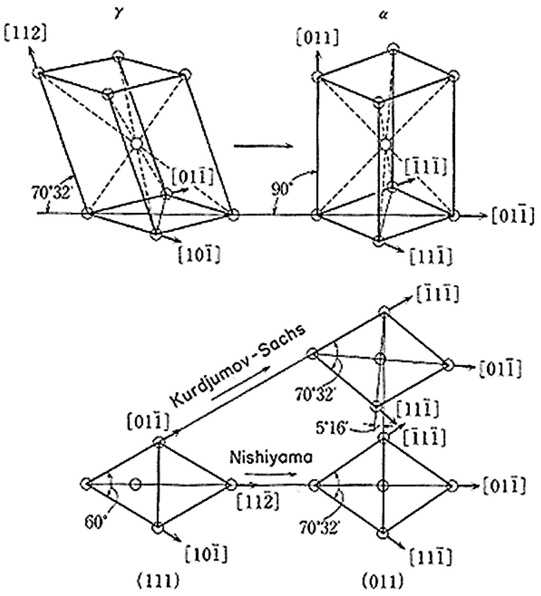
Figure 4.
Burgers’ model of bcc-hexagonal close-packed (hcp) transformation. Reprinted from [29] with permission from Elsevier. The two simultaneous shears are marked by the red ellipses.
Figure 4.
Burgers’ model of bcc-hexagonal close-packed (hcp) transformation. Reprinted from [29] with permission from Elsevier. The two simultaneous shears are marked by the red ellipses.

Figure 5.
The use of shears in the phenomenological theory of martensitic transformations (PTMC). (a) Schematic view of an invariant plane strain (IPS), with the shear value s and the dilatation part δ perpendicularly to the shear plane; (b) combination of the IPS P1 (also called shape strain) with a simple shear P2 that generates the correct and well-oriented lattice RB. The simple shear P2 is compensated by a lattice invariant shear to get the correct shape P1. Reprinted from [39] with permission from Elsevier.
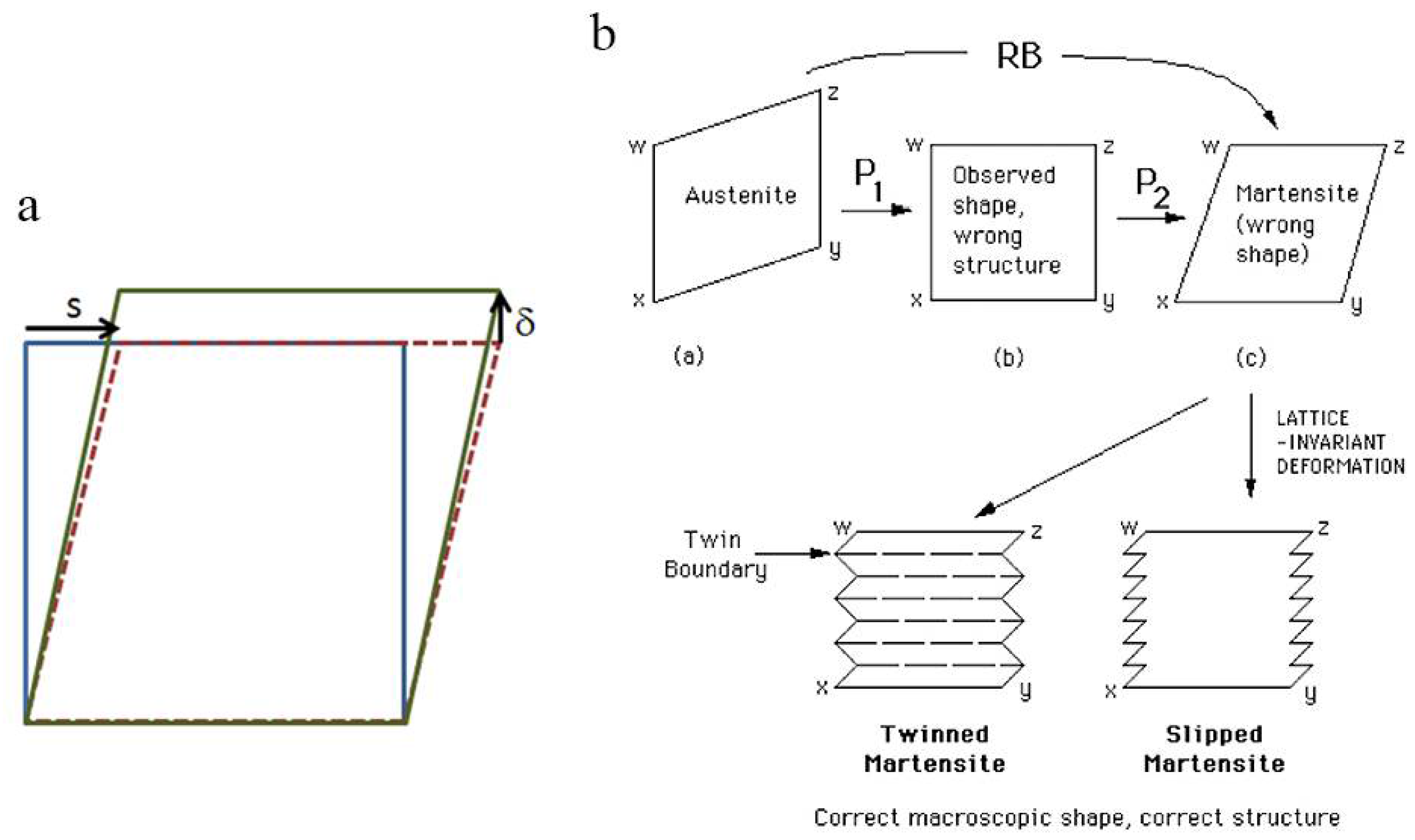
Figure 6.
Hard-sphere model proposed by Bogers and Burgers for the fcc-bcc transformation and fcc-fcc deformation twinning. The initial fcc structure (a) becomes, after distortion, a new twinned fcc structure (c). The bcc structure is at the midway between the two structures (b); however, additional shears are required to place the atoms at their correct positions. Reprinted from [53] with permission from Elsevier.
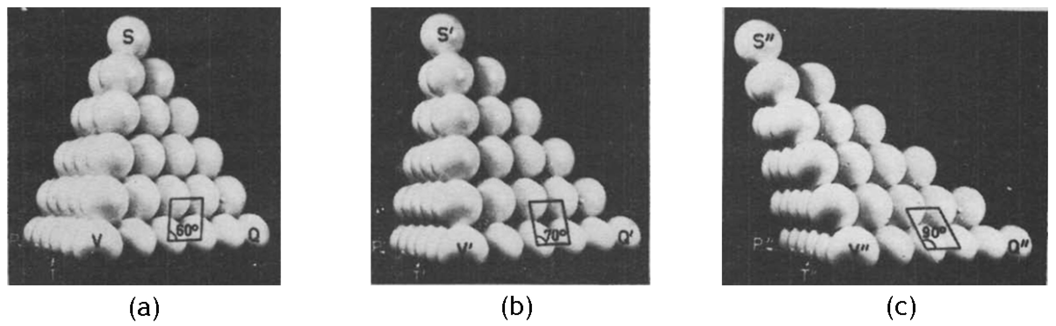
Figure 7.
Olson and Cohen’s refinement of Bogers and Burgers’ model. The α martensite is formed at the intersection of the two planar faults T/2 and T/3. Reprinted from [56] with permission from Elsevier.
Figure 7.
Olson and Cohen’s refinement of Bogers and Burgers’ model. The α martensite is formed at the intersection of the two planar faults T/2 and T/3. Reprinted from [56] with permission from Elsevier.

Figure 8.
Periodic functions τ with different slopes μ at the points τ = 0. (a) Sinusoidal function, μ = 1; (b) soft function, μ = 0; (c) infinitely rigid function, μ = ∞.
Figure 8.
Periodic functions τ with different slopes μ at the points τ = 0. (a) Sinusoidal function, μ = 1; (b) soft function, μ = 0; (c) infinitely rigid function, μ = ∞.

Figure 9.
Schematic two-dimensional (2D) representation of a collective displacement of atoms during deformation twinning, according to (a) simple shear (with internal friction) or (b) angular distortion (in a free crystal).
Figure 9.
Schematic two-dimensional (2D) representation of a collective displacement of atoms during deformation twinning, according to (a) simple shear (with internal friction) or (b) angular distortion (in a free crystal).
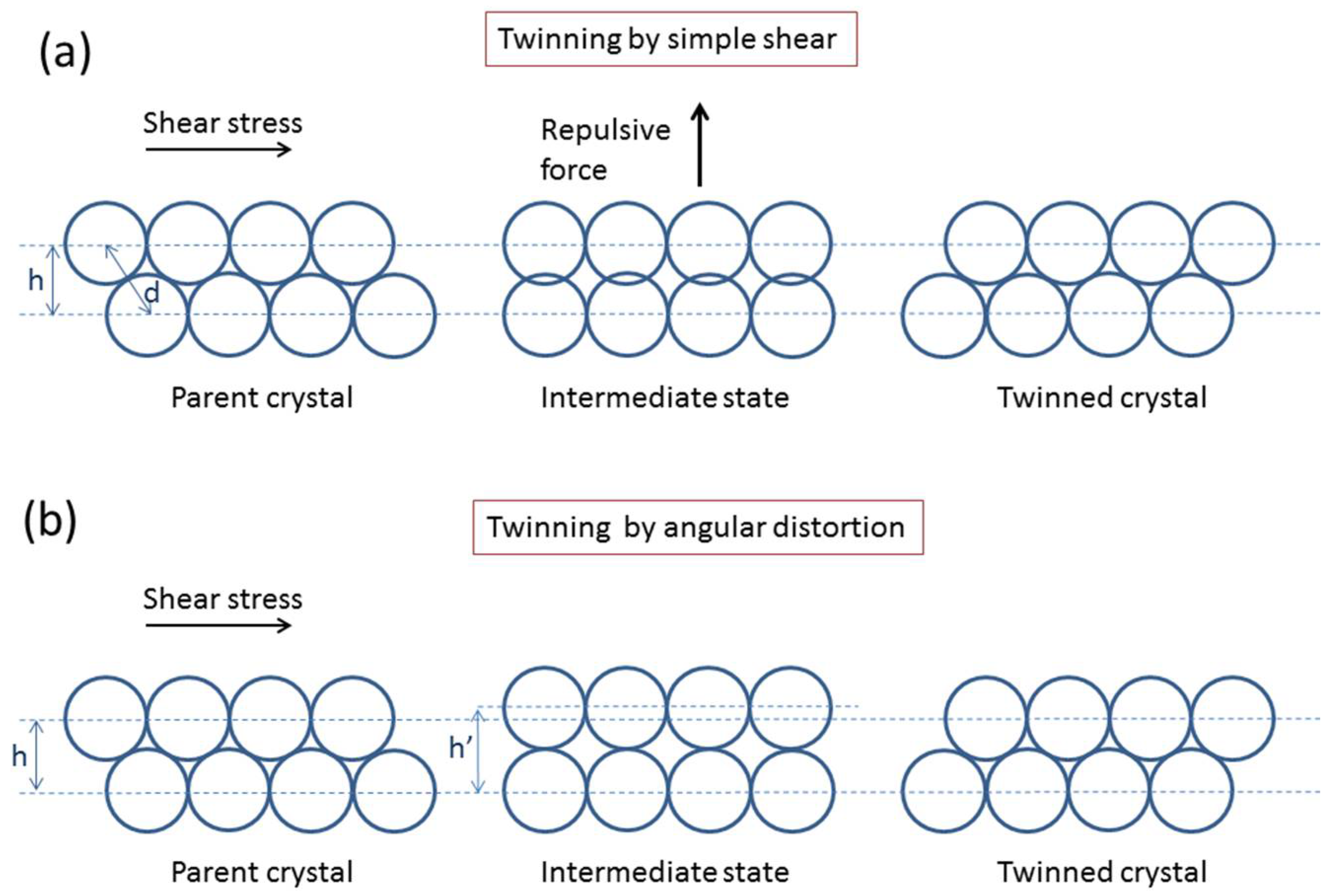
Figure 10.
Schematic representation of twinning dislocations and pole mechanism. (a) An early model made by Frank and Read explains the dislocation “multiplication” in a crystal, from Cottrell’s book [54]; (b) this model was used by Cottrell to explain how dislocations can build twins; (c) Scheme of the pole mechanism proposed by Venables, adapted from [73].
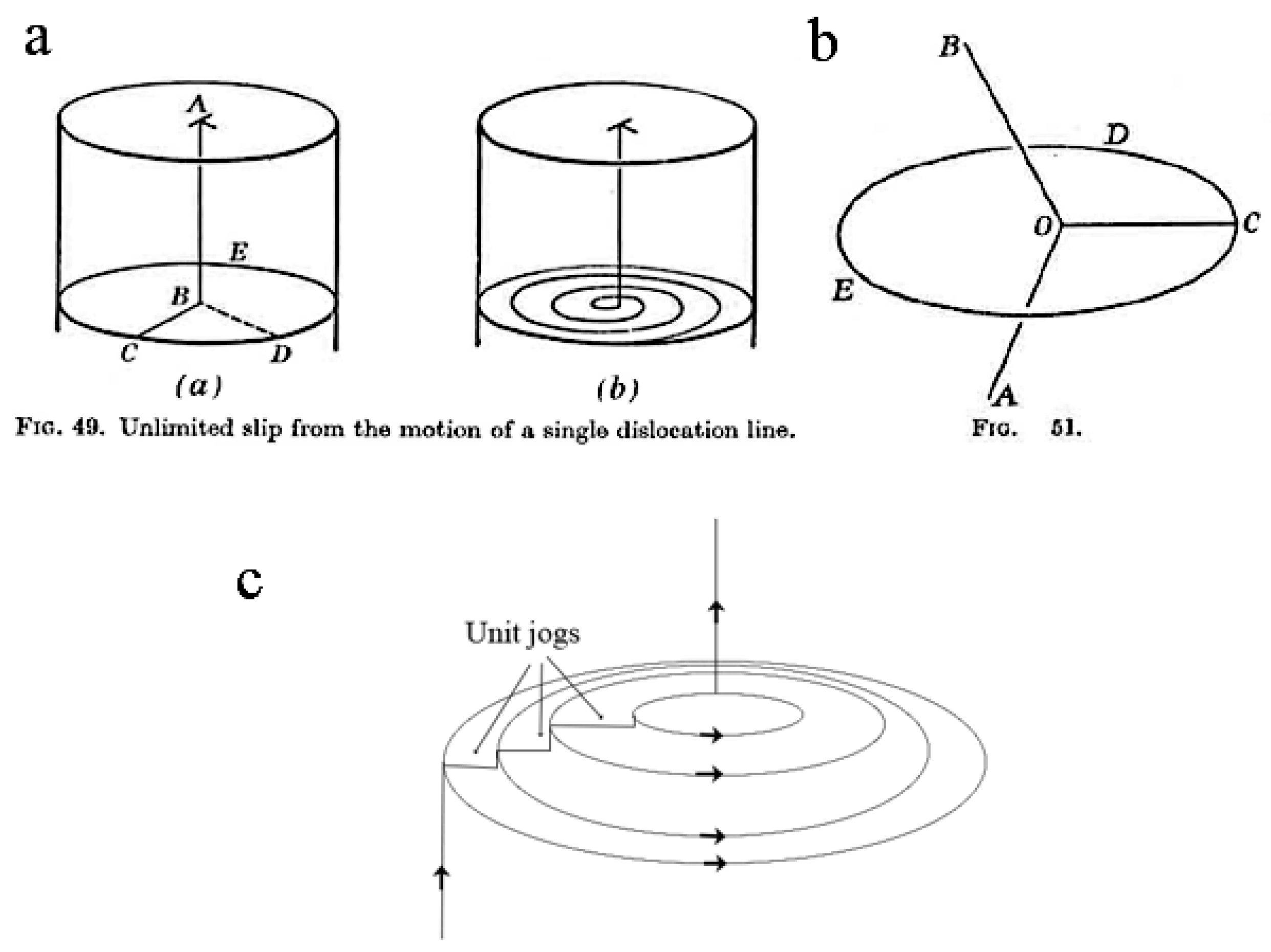
Figure 11.
TEM image of dislocation pileups in front of micro-twins presented as “twinning dislocations”, (a) in an Fe–Mn–Si–Al Transformation Induced Plasticity (TRIP) steel, from [74]; and (b) in a tetragonal Ni–Mn–Ga alloy. Reprinted from [79] with permission from Elsevier.

Figure 12.
Schematic representation of a 2D hexagonal ⟶ square displacive transformation, viewed as a “transformation wave”. The square phase is stabilized by a chemical reduction of energy or by mechanical work. (a) Initial hexagonal phase; (b) the atoms in a small area at the center (initially filled in blue) move collectively to form the square martensite phase (in red). An accommodation zone (in orange) is created between the parent hexagonal and the martensite square phases. The accommodation takes here the form of a progressive 60° ⟶ 90° rotation; (c) the transformation wave propagates at a high velocity, and continues forming the martensite phase; the previous accommodation zone becomes martensite, and a new accommodation zone is formed in front of the wave.

Figure 13.
Elastic and plastic accommodation zone around the martensite product in a parent grain of a polycrystalline material. (a) During the transitory stages of the martensite propagation, the parent/martensite incompatibilities can be spread to be elastically accommodated, and martensite can be formed as an acoustic wave; (b) when the martensite size becomes comparable to the grain size, the incompatibilities must be plastically accommodated.
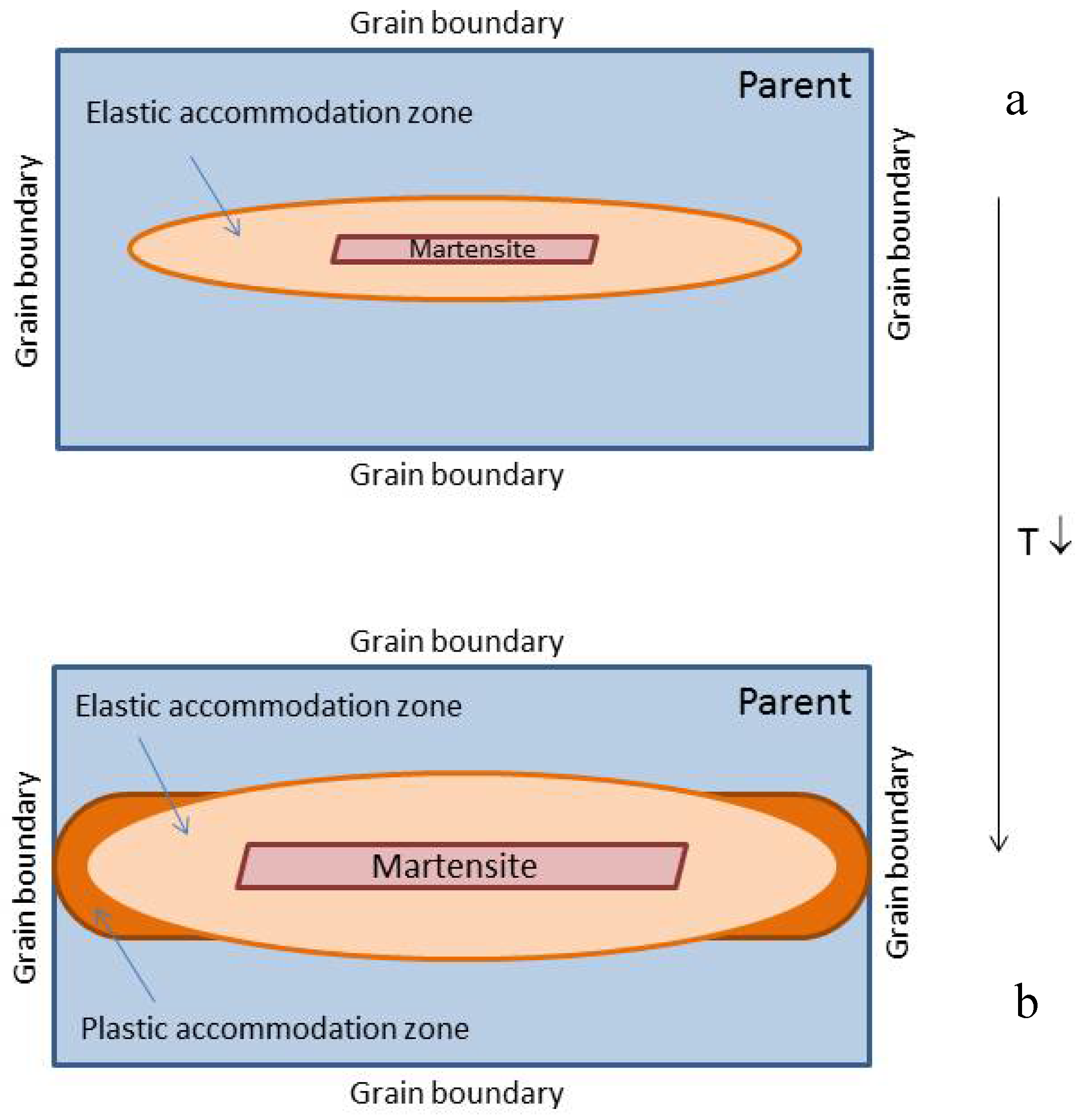
Figure 14.
Angular distortive model, (a) with hard-spheres; (b) with elastic-hard spheres.

Figure 15.
Volterra cut for a negative wedge disclination, where material is inserted (a–c), and alternative Volterra cut for a positive wedge disclination, where material is removed (d–f). Figure and caption reprinted from Müllner and King [102] with permission from Elsevier.
Figure 15.
Volterra cut for a negative wedge disclination, where material is inserted (a–c), and alternative Volterra cut for a positive wedge disclination, where material is removed (d–f). Figure and caption reprinted from Müllner and King [102] with permission from Elsevier.

Figure 16.
Hexagonal–square transformation with PTMC.
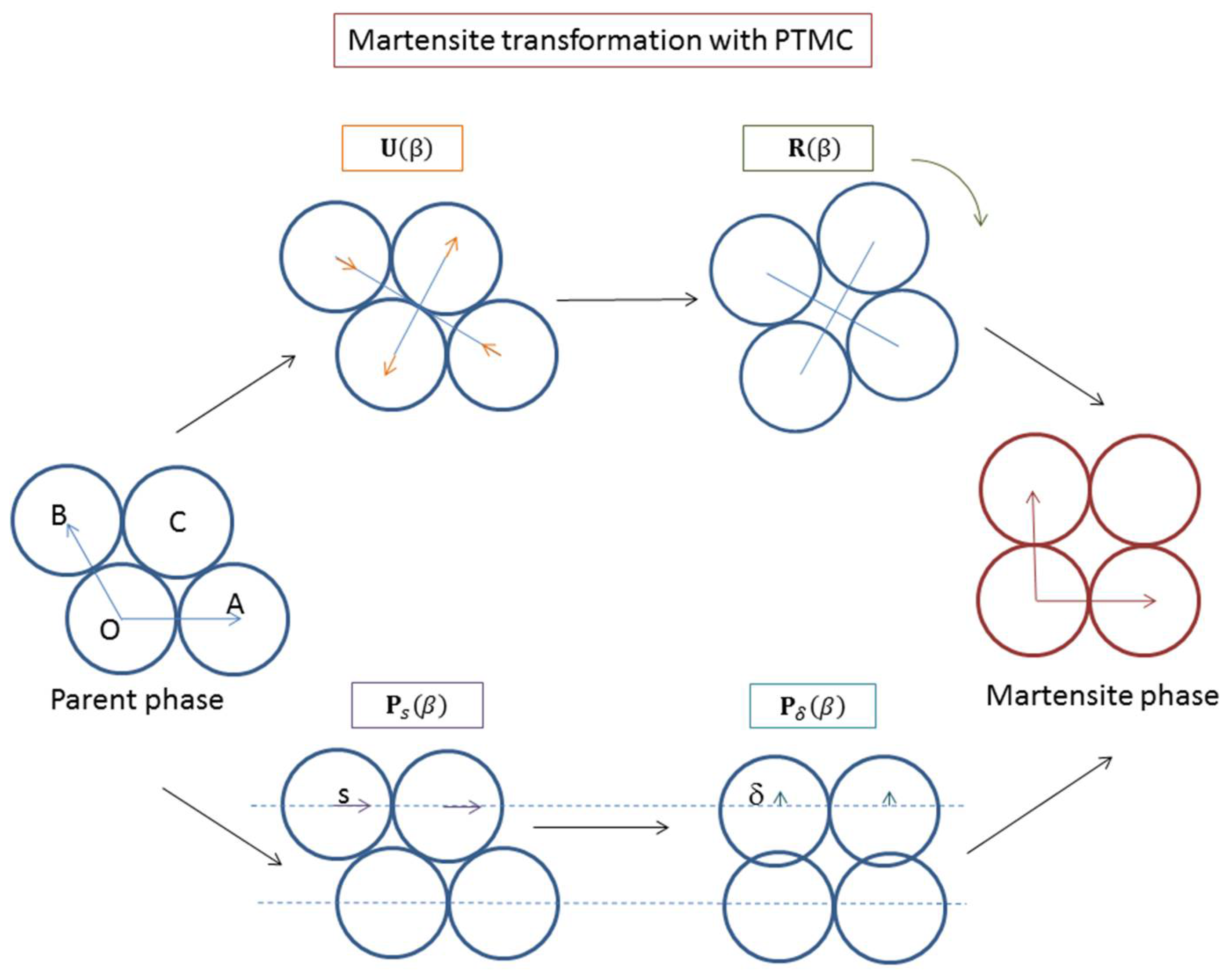
Figure 17.
Hexagonal–square transformation with angular distortion.

Figure 18.
Reconstruction of the parent grains from EBSD maps. (a) Initial EBSD map of fully martensitic Fe–0.1C-9Cr–1Mo–0.4Si steel; (b) prior parent austenitic grains, reconstructed with the software ARPGE. The orientations of the austenitic grains and those of the martensitic grains they contain are plotted in the pole figures, with the calculated <111>γ directions in red and the experimental <110>α directions in blue.

Figure 19.
Continuous gradients of orientations inside bcc martensitic grains. (a) Simulations of the pole figures made with 24 KS variants and two rotations A and B, with angular range 0–5° (left column), compared to the experiments (right column), from [114]; (b) RGB coloring of the Pitsch, KS, and NW ORs inside the martensitic grains of the EMT10 steel shown in 0. Reprinted from [115] with permission from Elsevier.

Figure 20.
Bain distortion with hard-spheres. (a) Initial fcc lattice; (b) same crystal with hard spheres. The direction of the contraction axis along a <100> direction is marked by the white arrows. (c) Final distorted crystal, which is half a bcc crystal cut on a (110) plane; (d) Initial fcc crystal and final bcc crystal after Bain distortion. Movie at http://lmtm.epfl.ch/research.

Figure 21.
KS distortion explained with hard-spheres. The continuity is given by a unique parameter, the angle, β = (PO, PK) that changes from 60° (bcc) to 70.5° (fcc). Movie at http://lmtm.epfl.ch/research.
Figure 21.
KS distortion explained with hard-spheres. The continuity is given by a unique parameter, the angle, β = (PO, PK) that changes from 60° (bcc) to 70.5° (fcc). Movie at http://lmtm.epfl.ch/research.

Figure 22.
Hard-sphere model of (a) fcc-fcc deformation twinning and (b) fcc-bcc martensitic transformation. The distance h is the distance between the planes, initially POK = (111)γ. This distance changes during the transformation process. Both fcc-fcc twinning and fcc-bcc martensitic transformations are modelled as functions of a unique angle of distortion, noted η and β, respectively. In both transformations, the dense plane POK and the dense direction PO remain untilted. Reprinted from [123] with permission from Elsevier.
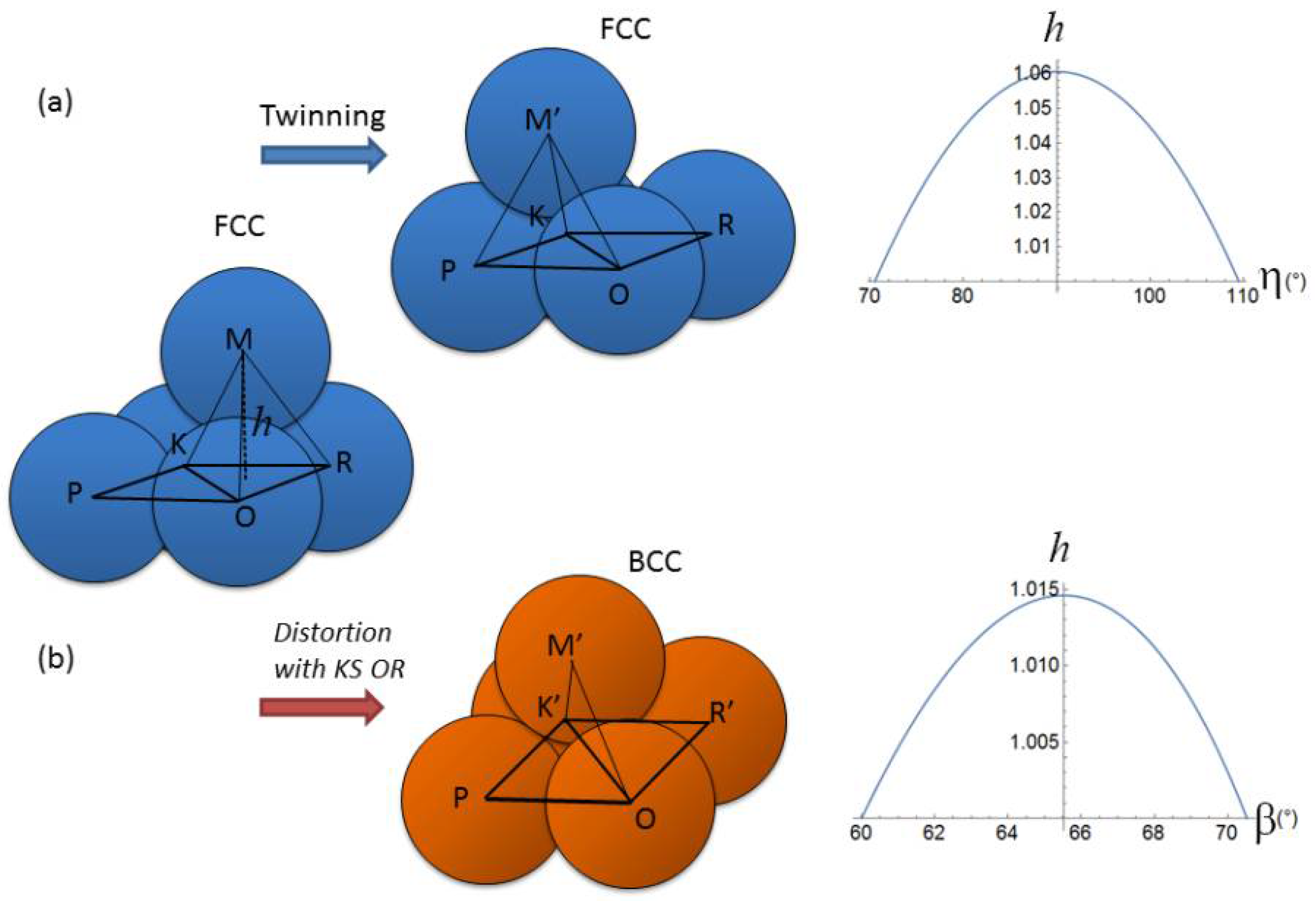
Figure 23.
Representation of the fcc-bcc distortion with the KS OR. The volume change is entirely due to the angular distortion in the plane POK ⟶ POK’, for which β = (PO, PK) increases for 60° to 70.5°.
Figure 23.
Representation of the fcc-bcc distortion with the KS OR. The volume change is entirely due to the angular distortion in the plane POK ⟶ POK’, for which β = (PO, PK) increases for 60° to 70.5°.

Figure 24.
Continuous distortion model of the fcc-bcc transformation on a (225) habit plane. This plane, which is only untilted during the formation of one variant, becomes an IPS when two twin-related KS variants are formed together. The atoms of the fcc crystal are in green, and those of the two final twin-related bcc variants are in red and blue. Movie available at https://www.nature.com/article-assets/npg/srep/2017/170120/srep40938/extref/srep40938-s1.avi. From [124].

Figure 25.
Interpretation of the surface relief formed by an fcc-bcc transformation. (a) Image made by atomic force microscopy of bainite plates, and (b) their interpretation by a shear mechanism. Reprinted from [128] with permission from Springer Nature. (c,d) Alternative explanation with an angular distortive mechanism. Surface (c) before transformation, and (d) after transformation; the tent-shape is compatible with an intra-planar distortion of the habit plane (without rotation).
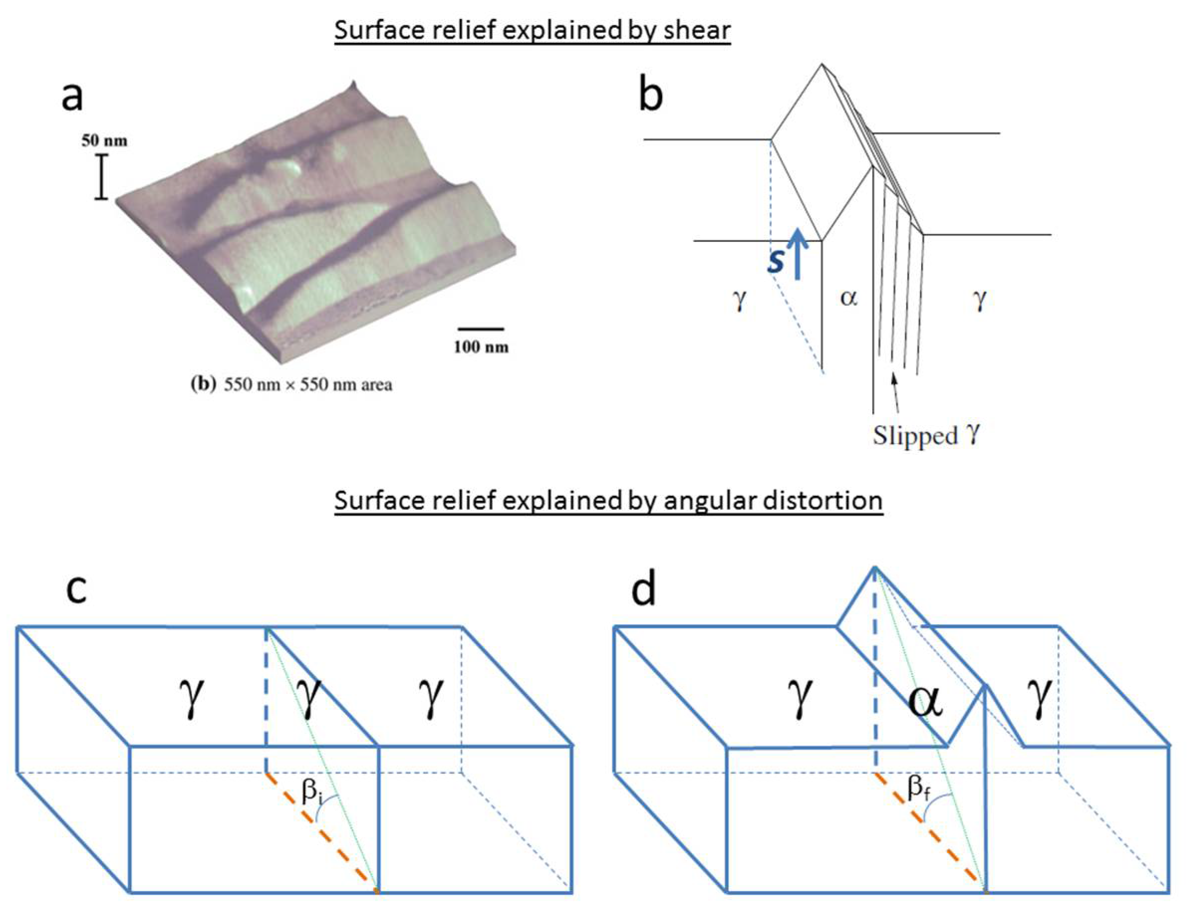
Figure 26.
Phase transformations in the fcc-hcp-bcc system. (a) As represented by Burgers in 1934 [29]; (b) planar representation of the fcc, bcc, and hcp structures. The positions l = 1 and l = 2 represent the level of the atoms in their stacking, perpendicular to the dense planes (11)γ//(10)α//(001)ε. Reprinted from [123] with permission from Elsevier.

Figure 27.
Snapshots of 3D simulation movies of (a) an fcc ⟶ bcc martensitic transformation. (b) fcc ⟶ fcc mechanical twinning. (c) fcc ⟶ hcp martensitic transformation, with, in blue, the initial parent fcc cube with its {100}γ facets; in red, the resulting transformed daughter crystals; and in yellow, the intermediate states stopped at midway (half of the maximum distortion angle). The black arrow represents the invariant line PO, and the white arrow the direction PK (also invariant for the fcc ⟶ hcp and fcc ⟶ fcc transformations). Reprinted from [123] with permission from Elsevier.
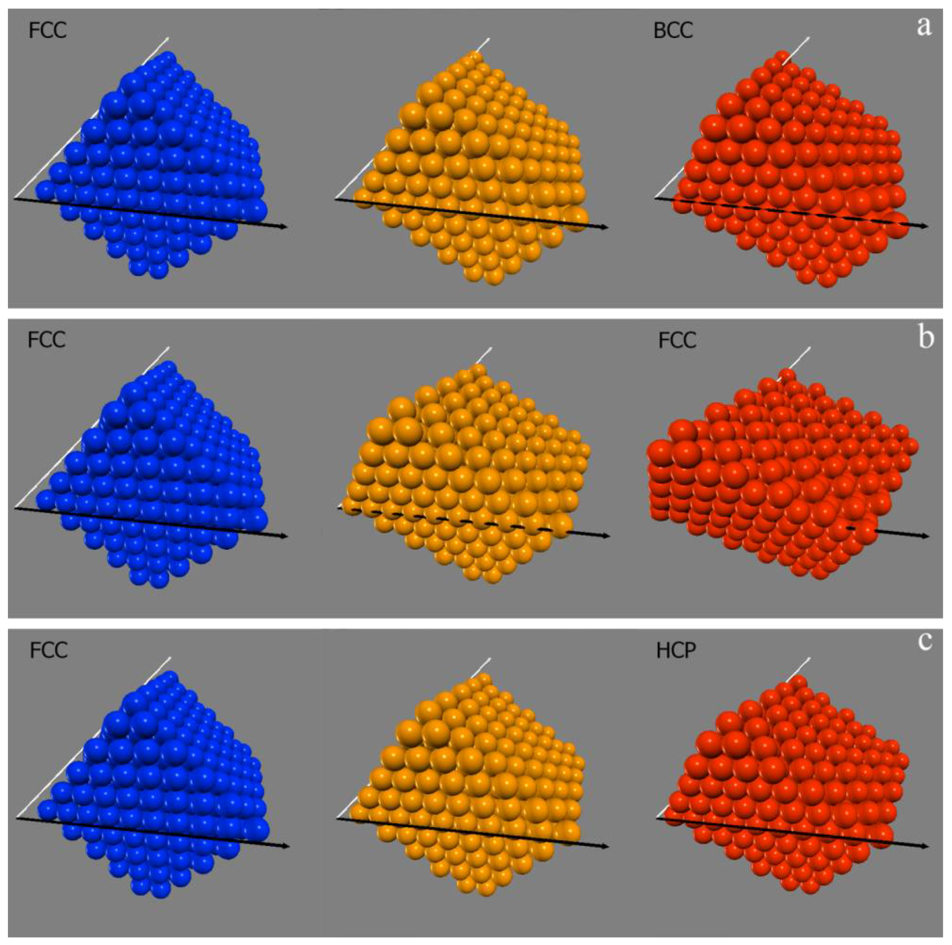
Figure 28.
Hard-sphere displacive model of extension twinning in magnesium. (a) Unit cell with labels O, X, M, N, Z, and T given to the magnesium atoms. (b) Schematic view of the atomic displacements associated with a stretch distortion; (c) obliquity ξ of the {012} plane that should be compensated for; (d) evolution of the distance OV belonging to the {012} plane; and (e) change of the unit volume during the distortion process, as functions of κ, the cosine of the angular parameter η. Adapted from [130].

Figure 29.
Interaction work during a tensile stress along the z-axis of a parent crystal, tilted by an angle Φ around the x-axis and rotated by an angle θ around the n-axis (normal to the twinning plane), with (a–c) for extension twinning in hcp metals, and the x-axis being the [100] axis. (d–f) For fcc-fcc deformation twinning, the x-axis is the [10] axis. (a,d) Interaction work Wf calculated with the complete distortion (simple shear) matrix. Wf is proportional to the usual Schmid factor. (b,e) Interaction work Wi calculated with the intermediate distortion matrix corresponding to the maximum volume change. (c,f) Schematic view of the orientation of the parent crystal. The distortion matrix of extension twinning in hcp metal is given in [130]. The distortion matrix for fcc-fcc deformation twinning is given in [123].
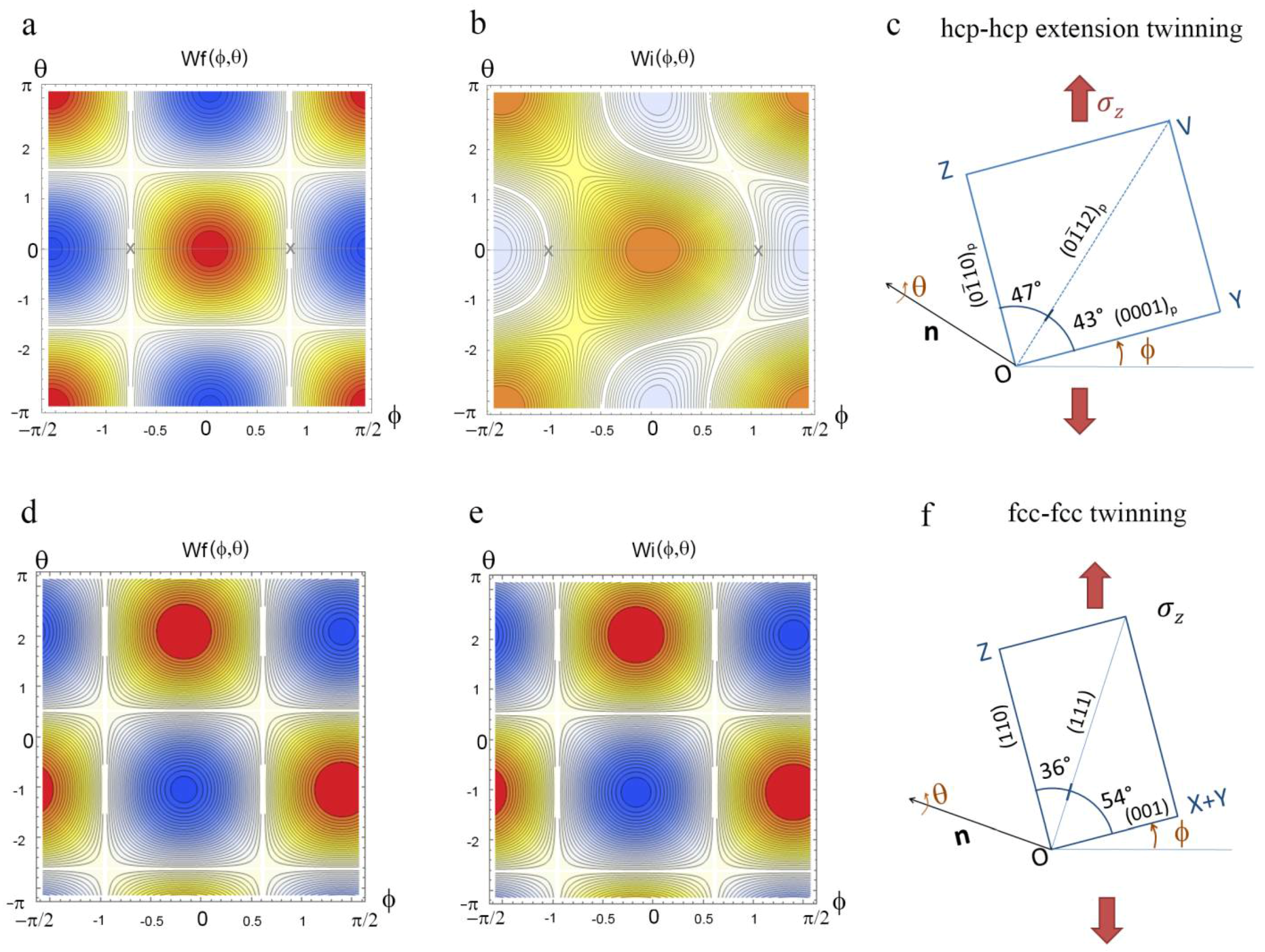
Figure 30.
Shuffle models of extension twinning in hcp metals proposed by (a) Wang et al., and by (b) Liu et al. Reprinted from [137] and from [131], respectively, with permission from Nature Publishing Group.

Figure 31.
EBSD maps of lenticular deformation twins, (a) formed in recrystallized pure (hcp) magnesium; and (b) in a (fcc) TWIP steel (kindly given by K. Zhu, ArcelorMittal). The twin boundaries are marked in red; they are identified by the misorientations (87° ± 5°, [001]hex) and (60° ± 5°, <111>fcc) in (a,b), respectively.
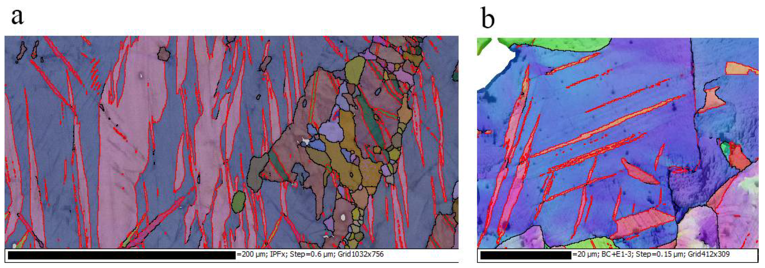
Figure 32.
Snapshots of three states during the formation of a (56°, a) contraction twin on the (011) plane in magnesium, simulated with the displacive hard-sphere model. (a) Initial hcp crystal; (b) intermediate state at midway; (c) newly formed hcp crystal. This figure is made to help understand the crystallographic exchange between the basal plane and the (011) plane. Reprinted from [147] with permission from the International Union of Crystallography.
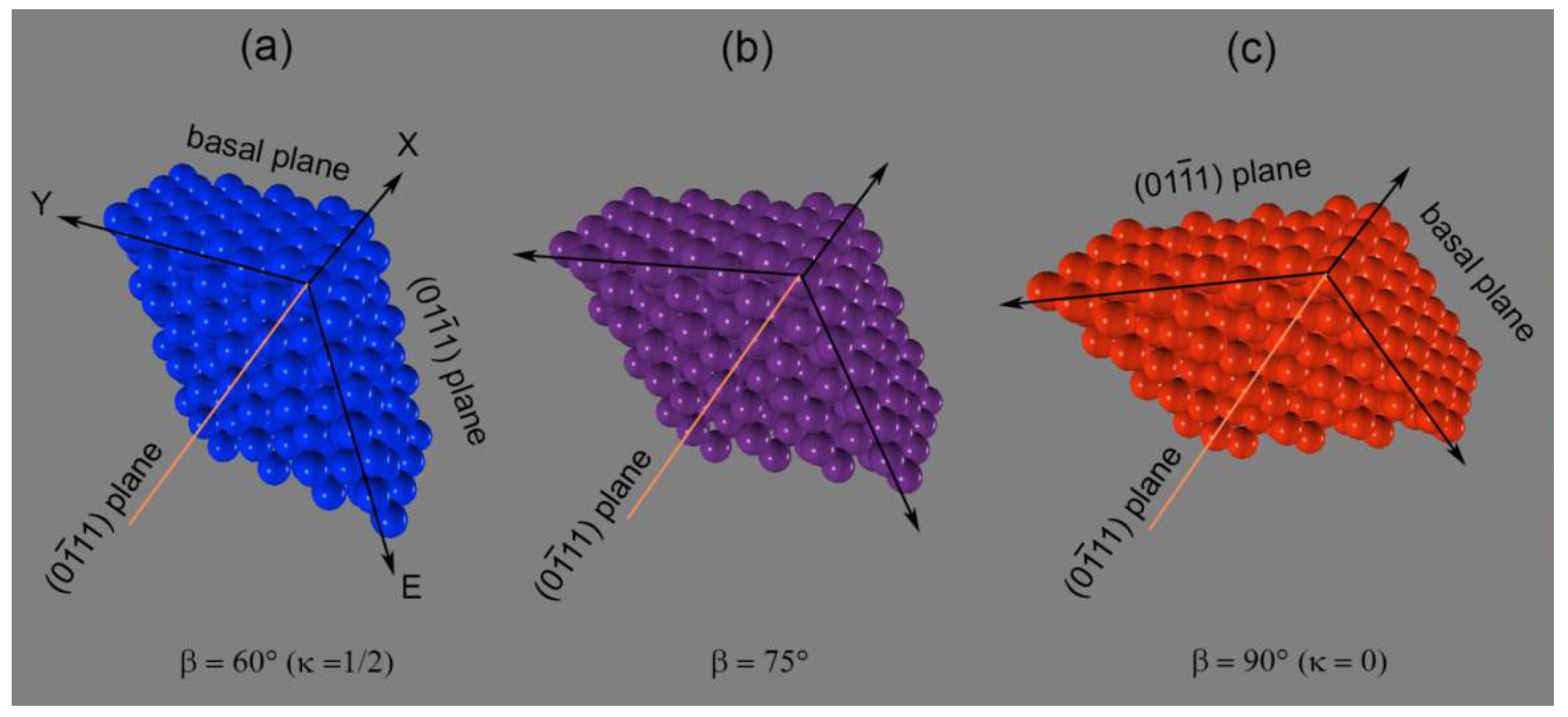
Figure 33.
Kronberg’s model of extension twinning in hcp metals. (a) Initial crystal with the “hard-sphere” atoms projected along the [010]hex direction, (b) corresponding lattice, (c) lattice distortion during twinning, and (d) lattice distortion and atomic displacements during twinning. Reprinted from [154] with permission from Elsevier.

Figure 34.
The free energy F function of the order parameter ξ and temperature T, and the order parameter function of the temperature T, in the case of (a,b) second order transitions, or of (c,d) first order transitions.
Figure 34.
The free energy F function of the order parameter ξ and temperature T, and the order parameter function of the temperature T, in the case of (a,b) second order transitions, or of (c,d) first order transitions.
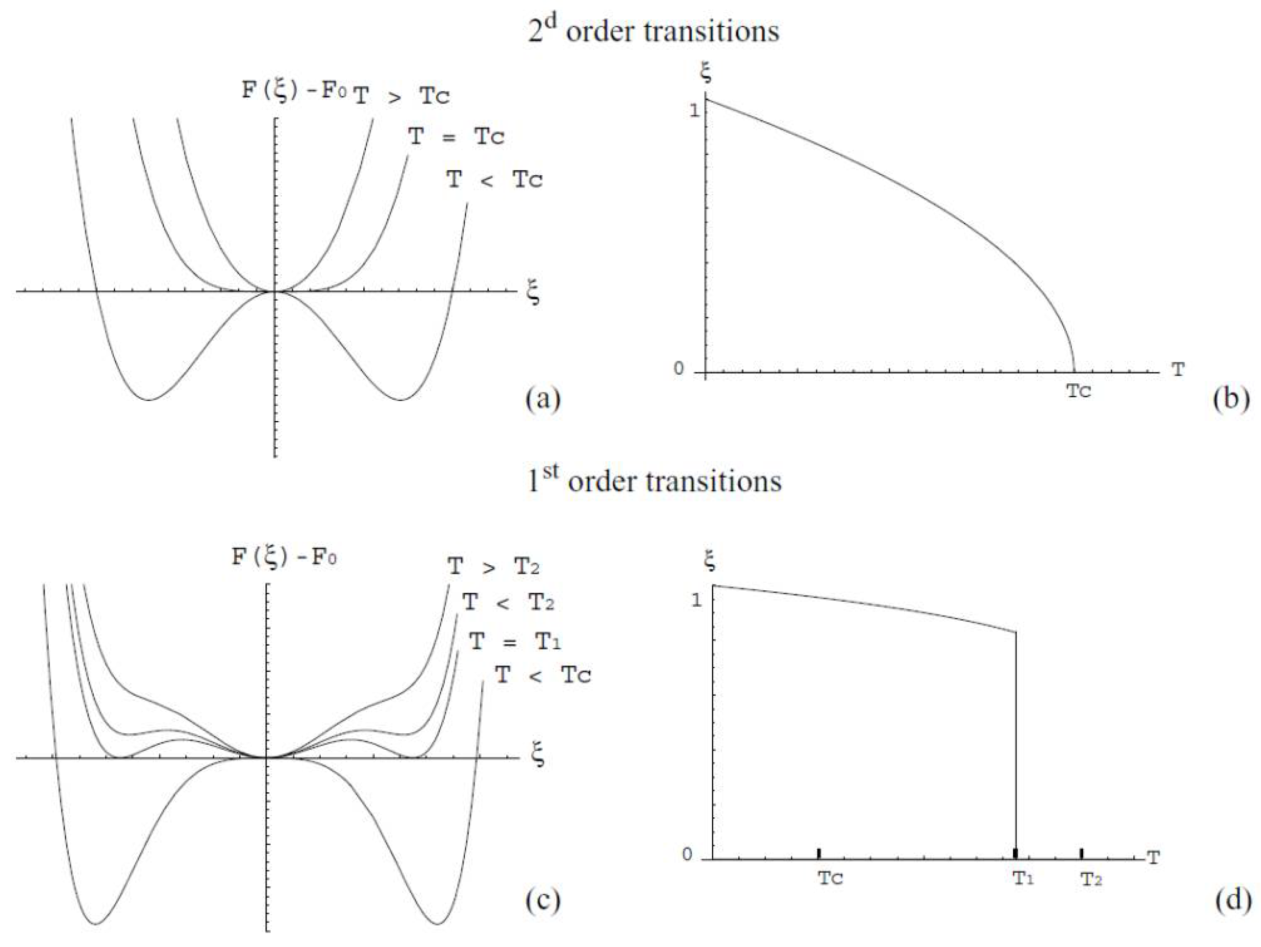
Figure 35.
Ramp function for the angular parameter β of the lattice distortion transformation D(β).

Figure 36.
Quasi-elastic lattice distortion during the (hexagonal ⟶ square) transformation of a free crystal. (a) Initial parent hexagonal phase, (b,c) intermediate states of the formation of the daughter square lattice inside the parent hexagonal lattice (the retained parent hexagonal phase can be identified close to the surface), and (d) daughter square phase after complete transformation. The initial circular shape of the crystal became elliptic after transformation. There is no “twinning dislocation” involved in the mechanism.
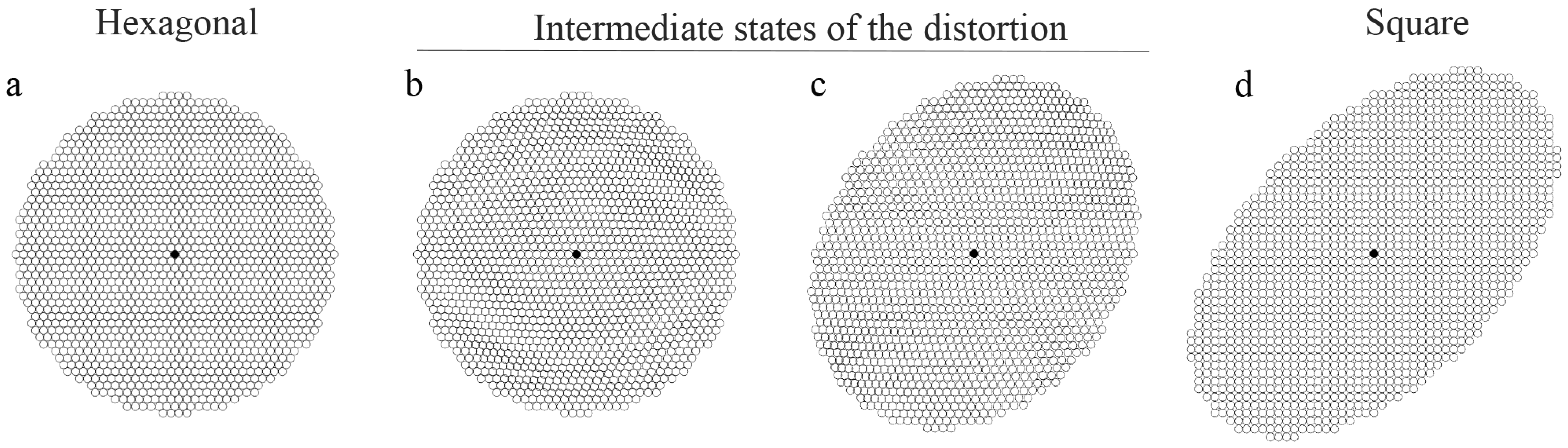
© 2018 by the author. Licensee MDPI, Basel, Switzerland. This article is an open access article distributed under the terms and conditions of the Creative Commons Attribution (CC BY) license (http://creativecommons.org/licenses/by/4.0/).
Share and Cite
MDPI and ACS Style
Cayron, C. Shifting the Shear Paradigm in the Crystallographic Models of Displacive Transformations in Metals and Alloys. Crystals 2018, 8, 181. https://doi.org/10.3390/cryst8040181
AMA Style
Cayron C. Shifting the Shear Paradigm in the Crystallographic Models of Displacive Transformations in Metals and Alloys. Crystals. 2018; 8(4):181. https://doi.org/10.3390/cryst8040181
Chicago/Turabian StyleCayron, Cyril. 2018. "Shifting the Shear Paradigm in the Crystallographic Models of Displacive Transformations in Metals and Alloys" Crystals 8, no. 4: 181. https://doi.org/10.3390/cryst8040181
Note that from the first issue of 2016, this journal uses article numbers instead of page numbers. See further details here.