Systematics of the Third Row Transition Metal Melting: The HCP Metals Rhenium and Osmium

Abstract

The melting curves of rhenium and osmium to megabar pressures are obtained from an extensive suite of ab initio quantum molecular dynamics (QMD) simulations using the Z method. In addition, for Re, we combine QMD simulations with total free energy calculations to obtain its phase diagram. Our results indicate that Re, which generally assumes a hexagonal close-packed (hcp) structure, melts from a face-centered cubic (fcc) structure in the pressure range 20–240 GPa. We conclude that the recent DAC data on Re to 50 GPa in fact encompass both the true melting curve and the low-slope hcp-fcc phase boundary above a triple point at (20 GPa, 4240 K). A linear fit to the Re diamond anvil cell (DAC) data then results in a slope that is 2.3 times smaller than that of the actual melting curve. The phase diagram of Re is topologically equivalent to that of Pt calculated by us earlier on. Regularities in the melting curves of Re, Os, and five other 3rd-row transition metals (Ta, W, Ir, Pt, Au) form the 3rd-row transition metal melting systematics. We demonstrate how this systematics can be used to estimate the currently unknown melting curve of the eighth 3rd-row transition metal Hf.

1. Introduction

Uncertainty in experimental stress conditions is an important source of error in measurements of phase equilibria and physical properties at deep Earth pressures. This error is evident in the range of reported pressures for key mantle phase transitions such as the perovskite–post-perovskite boundary in MgSiO${}_3$. Accurate pressures are also necessary for measurements of the equation of state and compressibility of different materials. Differences of up to 15% have been observed among equation of state measurements for materials such as MgSiO${}_3$ post-perovskite and iron largely due to pressure scale differences at Mbar pressure. Advances in high-pressure techniques require standards which are applicable at multi-Mbar pressures.

An ideal pressure standard is inert and compressible, with a simple crystal structure and strong X-ray diffraction pattern. Ideally, it should have no phase transitions over the experimental pressure range. In reality, it may have phase transitions, but its phase diagram should be relatively simple, with all the solid phases being described by simple and well-defined equations of state. Both gold and platinum have been in focus of high-pressure research for several decades as primary equation of state standards. Supposedly large pressure and temperature stability ranges of the face-centered cubic (fcc) phases of the third row transition metals Au and Pt and their large isothermal compressibility make them very attractive materials to be used as pressure markers above 1 Mbar. However, the newly discovered structural transformation in gold [1] severely limits the applicability of the Au standard. Likewise, the structures instability in Pt at high pressure $\left(P\right)$ and temperature $\left(T\right)$ [2] limits the applicability of the Pt standard to low T.

Another consideration in pressure calibrant choice is overlap of diffraction peaks of the standard with those of the sample. For Au and Pt (as well as, e.g., another potential pressure marker MgO) that have fcc structure, their diffraction peak positions are similar at Mbar conditions. In this respect, another pair of the third row transition metals, namely, Re and Os, that have hexagonal close-packed (hcp) structure, may offer potential to be a useful alternative to fcc standards. At present, the phase diagrams of either Re or Os are virtually unknown. We address the issue of their phase diagrams (specifically, their melting curves) in this paper. We calculate the melting curves of Re to 3.5 Mbar and of Os to 5 Mbar using ab initio quantum molecular dynamics (QMD) simulations.

In what is now following, we summarize the existing information on both Re and Os that can be found in the literature.

1.1. Rhenium

The equation of state (EOS) of solid Re has been extensively studied to P as high as 640 GPa [3], and there are isothermal compression data at Ts up to 3000 K [4]. Comparison of the $T=0$ free energies of candidate crystal structures for Re shows that hexagonal close-packed (hcp) is the most stable structure up to at least a compression of two; face-centered cubic (fcc), the closest structure to hcp, is 4 to 12 mRy/atom (55–165 meV/atom) higher in energy [5]. The $T=0$ fcc-hcp free energy difference is a quasi-linear function of P up to ∼1000 GPa: $\Delta F_{\mathrm{fcc}-\mathrm{hcp}}\left(P\right)\approx 55+0.11P$ meV/atom. Unless a free energy difference becomes sufficiently large (typically $\stackrel{>}{\sim }0.1$ eV/atom, which corresponds to P∼ 400 GPa for Re), it can be overcome by the entropy term at finite T, hence we expect fcc-Re to become energetically competitive with hcp-Re with increasing T over some limited range of P.

In 2012, Yang, Kandikar, and Boehler (YKB) carried out DAC measurements of the melting temperature of Re to 50 GPa [6]. Their melting curve is quasi-linear with a slope of 17 K/GPa, which is 2.3 times smaller than the slope (40 K/GPa) of the melting curve measured by Vereshchagin and Fateeva (VF) in 1975 using electrical heating in a belt apparatus to 8 GPa [7]. Other, theoretical, values for this slope are 58 K/GPa [8] and 29.2 K/GPa [9,10]. If 17 K/GPa were the correct value of the initial slope of its melting curve, Re would be unique among the transition metals of the third period since the melting curves of the other metals in this group that have been reliably determined either experimentally or theoretically, or both, have initial slopes in the range 40–55 K/GPa: ∼55 for Au [11,12,13], ∼50 for Ir [14], ∼45 for Ta [15] and W [16], and ∼40 for Pt [2]. Below we show that it is the VF melting curve that is correct, and with which our ab initio QMD simulations are in excellent agreement, rather than the recent YKB DAC curve which in fact includes part of the Re s-s (specifically, hcp-fcc) phase boundary.

1.2. Osmium

Comparison of the $T=0$ free energies of candidate crystal structures for Os shows that hexagonal close-packed (hcp) is the most stable structure up to at least a compression of two; face-centered cubic, the closest structure to hcp, is ∼10 mRy/atom (∼0.14 eV/atom) higher in energy [17]. The very recent experimental study [18] reveals that Os retains its hcp structure upon compression to ∼800 GPa. Hence, we assume that in the pressure range considered in this work Os is a single-phase (hcp) material.

The equation of state (EOS) of solid osmium has been extensively studied [19]. The very recent experimental data go up to a pressure of 700 GPa [18], and there are isothermal compression data at temperatures up to 3000 K [20], but its melting curve, $T_m\left(\rho \right)$ or $T_m\left(P\right)$, has never been measured. A theoretical melting curve of Os to 800 GPa [17] has been constructed on the basis of first-principles calculations of the Grüneisen parameter, $\gamma \left(\rho \right)$, and the use of the Lindemann formula for the melting temperature as a function of density, i.e., $d\ln T_m\left(\rho \right)/d\ln \rho =2[\gamma \left(\rho \right)-1/3].$ With this theoretical melting curve converted into the P-T coordinates, using the corresponding EOS, melting on the Hugoniot is predicted to occur at ∼450 GPa and ∼9200 K [17]. Most recently, Kulyamina et al. [21] analyzed all of the isobaric-heating data on Os available in the literature and extracted the initial slope of the Os melting curve: $d{T}_m\left(P\right)/dP=40.4$ K/GPa. We note that their determination is based on the Clausius-Clapeyron relation $d{T}_m/dP=\Delta V_m/\Delta S_m,$ but since neither the volume change at melt, $\Delta V_m,$ nor the melting entropy, $\Delta S_m,$ are known from experiment, their values can only be estimated. Other, theoretical, values for this slope are 65 K/GPa [8] and 53.4 K/GPa [9,10].

2. Z Method Calculations

In the present work we determine the melting curves of rhenium to ∼350 GPa and osmium to ∼500 GPa using the Z method which we describe in what follows.

The Z method was developed to calculate melting curves using first-principles based software, specifically VASP (Vienna Ab initio Simulation Package); it was introduced and used for the first time in our paper on the ab initio melting curve of Mo [22]. The method has since been applied to the study of a large number of melting curves of different materials [23,24,25], and comparisons with experimental data on Pb [26], Ta [15], Fe [27], and Pt [28] at European Synchrotron Radiation Facility (ESRF) show good agreement. If a material has more than one thermodynamically stable crystal structure, the Z method yields the solid-liquid equilibrium boundaries of those structures. The phase having the highest solid-liquid equilibrium temperature over some pressure range is the most stable, thus the physical melting curve, including triple points, is the envelope of the solid-liquid equilibrium boundaries. We note that until recently, VASP could only be run for $NVE$ or $NVT$ ensembles, but with the release of the latest version, VASP5.3, we now have the option of running $NPT,$ hence the so-called 2-phase simulations are now an alternative to the Z method.

Figure 1 shows a typical Z isochore, there comprised of the three green segments AC-CD-DE. It can be approximately mapped out by performing a sequence of QMD runs at progressively higher temperatures and pressures, typically 6–8 points, starting in the solid (segment AB), progressing to the superheated (SH) solid (segment BC), and finally to the liquid (segment DE). If the total energy in a QMD run in the superheated solid is such that the equilibrium temperature $T<T_C$, the final state is on segment AC, but if $T>T_C$ the system melts and the final state is a point $(P_l,T_l)$ on segment DE above the melting curve (dark blue); a further increase in the initial system energy moves the final state up segment DE. Ideally, the QMD runs in the superheated solid would differ by only small temperature increments so that the upper vertex C would be precisely determined, and then a run starting from C would take the system to the point D on the melting curve, but generally this cannot be achieved in practice. The standard implementation of the Z method involves bounding the vertex D from below by the highest calculated state $(P_s,T_s)$ on solid segment AB, and from above by the lowest state $(P_l,T_l)$ on liquid segment DE. Then the melting point can be approximated as $(P_m,T_m)\approx$ $((P_s+P_l)/2,(T_s+T_l)/2)$. The true melting point must be close to $(P_m,T_m)$ because the actual melting curve crosses the box formed by $P_m\pm (P_l-P_s)/2$ and $T_m\pm (T_l-T_s)/2$.

3. QMD Simulations of the EOS and the Melting Curve of Os

Our Z method calculations are carried out using the QMD code VASP, which is based on density functional theory (DFT). We use the generalized gradient approximation (GGA) with the Perdew-Burke-Ernzerhof (PBE) exchange-correlation functional. We model Os using the electron core-valence representation [${}^{48}$Cd $4f^{14}]5p^{6}5d^{6}6s^2$, i.e., we assign the 14 outermost electrons of Os to the valence. The valence electrons are represented with a plane-wave basis set with a cutoff energy of 400 eV, while the core electrons are represented by projector augmented-wave (PAW) pseudopotentials.

3.1. T = 0 Isotherm

We first calculated the $T=0$ isotherm of Os. This was done by optimizing the value of $c/a$, i.e., determining the $c/a$ that minimizes the energy, at a fixed volume of a hexagonal supercell, and extracting the corresponding value of P. We used a $8\times 8\times 5$ (640-atom) supercell with a single $\mathsf{\Gamma }$-point. With such a large supercell, energy convergence to $\stackrel{<}{\sim }$2.5 meV/atom is achieved, which was verified by performing short runs with $2\times 2\times 2,$ $3\times 3\times 3$, and $4\times 4\times 4$ k-point meshes and comparing their output with that of the 640-atom run with a single $\mathsf{\Gamma }$-point. This introduces additional uncertainty of ∼30 K for the numerical values of the corresponding $T_m$ which is small compared to the uncertainties of the Z method itself (75 K or 125 K, see below).

In the ab initio approach, the density of osmium at $(P,T)=(0,0)$ is 22.17 g/cc, whereas the experimental value is 22.66 g/cc [29]. Specifically, VASP predicts the lattice constants of the hexagonal unit cell to be (upon optimizing its $c/a$ ratio) $a=2.7319$ Å and $c=4.3134$ Å ($c/a=1.5789$), which corresponds to 22.17 g/cc. The experimental values are [30] $a=2.7315$ Å $c=4.3148$ Å ($c/a=1.5797$), and $\rho =22.661$ g/cc. Alternatively, with VASP, the experimental $(P,T)=(0,0)$ density of 22.66 g/cc corresponds to $(P,T)=(9.4$ GPa, $0)$. This 2.2% density mismatch, or 9.4 GPa pressure mismatch, is due to the specifc implementation of DFT, namely PBE, in our VASP simulations. In order to directly compare our QMD results to experiment, we will apply the 2.2% density correction (9.4 GPa pressure correction) to all VASP results in the $\rho$-T (P-T) plane. Specifically, we will multiply VASP densities by 1.022, or subtract 9.4 GPa from VASP pressures, whichever is relevant.

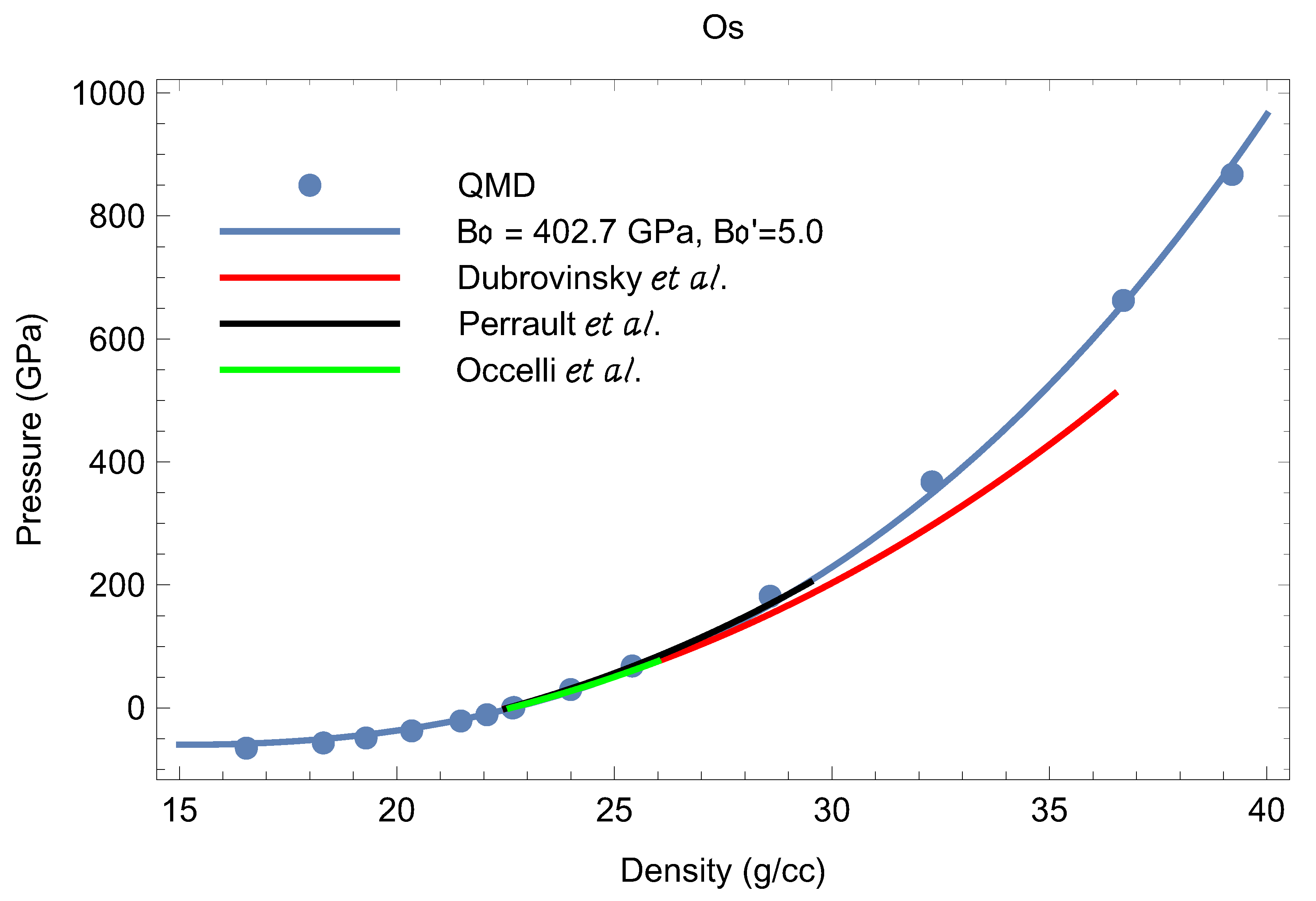
Our results on the $T=0$ isotherm, as well as the value of $c/a$ as a function of $P,$ are shown in Figure 2 and Figure 3, respectively. We note that each of the papers that discuss Os EOS data [18,19,20,31,32,33,34] uses the third-order Birch-Murnaghan (BM3) EOS

$$P\left(\rho \right)=\frac{3}{2}{B}_0\left({\left(\frac{\rho }{{\rho }_0}\right)}^{7/3}-{\left(\frac{\rho }{{\rho }_0}\right)}^{5/3}\right)\left[1+\frac{3}{4}(B_0^{\prime }-4)\left({\left(\frac{\rho }{{\rho }_0}\right)}^{2/3}-1\right)\right],$$

(1)

where $B_0$ and $B_0^{\prime }$ are the values of the bulk modulus and its pressure derivative at the reference point $\rho ={\rho }_0.$ Since the $P=0$ values of the density of Os at $T=0$ and 300 K differ by ∼0.3% (22.66 vs. 22.59 g/cc [29]), and $T=300$ K introduces a negligibly small thermal pressure correction, the $T=0$ and $T=300$ K isotherms can be described by the same values of $B_0$ and $B_0^{\prime }$. Consequently, we can compare room-temperature isotherm data to our zero-temperature isotherm as determined from QMD. A comparison is shown in Figure 2. It is seen that BM3 with $B_0^{\prime }=5$ fits both the experimental and QMD data up to ∼200 GPa as well as the QMD data at higher $P.$ Our best fit to the QMD data in the whole pressure range gives $B_0=415.0$ GPa and $B_0^{\prime }=4.87.$

3.2. $c/a$ Ratio as a Function of P

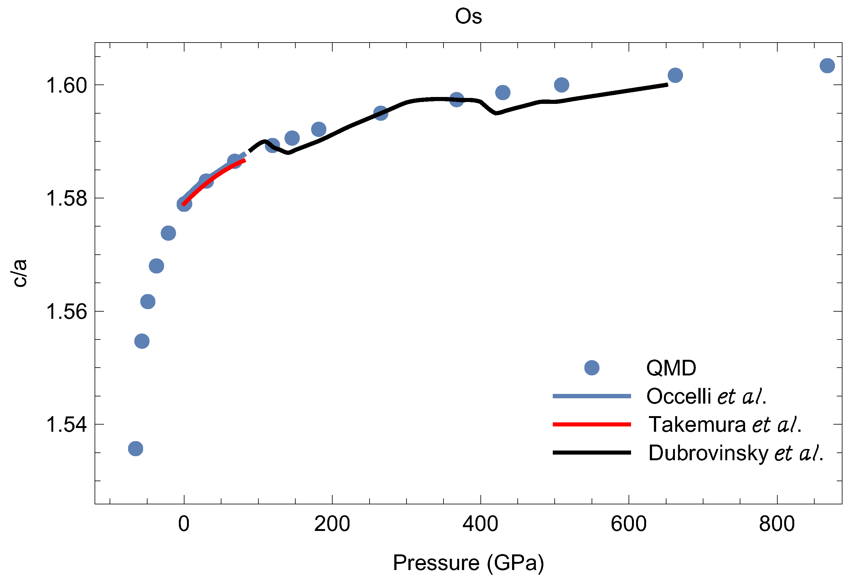
Based on their experimental results on $c/a$ as a function of $P,$ Occelli et al. [31] suggested the existence of an isostructural phase transition in Os at about 25 GPa associated with an anomaly in the compressibility. This anomaly was in turn associated with a discontinuity in the first pressure derivative of the $c/a$ ratio which may arise from the collapse of the “small hole-ellipsoid” [31] in the Fermi surface near the L point. Subsequent experimental studies did not confirm this $c/a$ anomaly [19,32,35]. However, the very recent experiments by Dubrovinsky et al. [18] reveal two different anomalies, around 150 and 400 GPa, each of which represents a small, ∼0.2%, reduction in the $c/a$ value (Figure 3). As discussed in [18], the first of these two anomalies may be the signature of a topological change in the Fermi surface for valence electrons, while the second might be related to an electronic transition associated with pressure-induced interactions between core electrons. No such $c/a$ anomalies are seen in our ab initio study (Figure 3). As noted in [18], in the case of Os, direct comparison between theory and experiment is not legitimate, because the calculations are carried out at $T=0$ whereas the experimental data are taken at room temperature. Moreover, for hcp metals, direct comparison between theory and experiment is generally nontrivial: in hcp metals the effect of the electronic transitions on the $c/a$ ratio should become visible at finite T due to the anisotropy of the thermal expansion of the hcp lattice. In any event, for these two anomalies, reductions in the $c/a$ value are so small that each of the corresponding pressures (related to the volume derivative of the total energy as a function of $c/a$ at fixed volume) only changes by a few tens of GPa. Therefore, even if they are real, these anomalies do not influence the room-T isotherm of Os that does not take them into account; consequently, they do not influence comparison of our cold EOS to this room-T isotherm. Finally, we note that the most recent expeimental EOS of Os [34] does not confirm the occurence of either of the two anomalies of Ref. [18].

3.3. Melting Curve

In contrast to previous melting curve calculations based on the Z method, here the method was utilized as closely as possible to the original concept, but at the expense of an extensive suite of QMD simulations. We calculated eight melting points. At a given density we performed a sequence of very long runs, each up to 25,000 time steps or 25 ps, with initial temperatures separated by relatively small increments: 150 K for the first three points on the Os melting curve and 250 K for the remaining five points. We performed 10 such runs for each of the first three points, and 14 runs for each of the remaining five points for a total of 100 runs and ∼2 million time steps. In the course of these extensive computer simulations, our strategy for detecting the melting point was as follows. The conversion of the initially ordered solid state into a disordered liquid during a QMD run was detected in one of three ways: (i) visual observation of atomic motion in the computational cell (vibrations around equilibrium sites in a solid vs. diffusion between the sites in a liquid); (ii) a drop in the value of the equilibrium T and the corresponding jump in the value of the equilibrium P; (iii) change in the radial distribution function (a long sequence of well-pronounced peaks in a solid vs. a few peaks in a liquid). If the system did not melt during the 25 ps of running time, we started the next run with an initial T higher by 150–250 K than the previous one, etc. The first run in which the system melts during the 25 ps of running time was assumed to correspond to the upper vertex C; during this run the complete melting process corresponding to the C→D transition in Figure 1 is usually observed. We refer to such a run as the melting run. With an even higher initial T, the system melts at an earlier time than in the melting run, and the duration of the melting process shortens; both the time when melting begins and the duration of the process decrease with increasing T, and for a sufficiently high initial T the system melts immediately. Examples of the QMD melting simulations using the Z method are shown in Figure 4, Figure 5, Figure 6 and Figure 7.

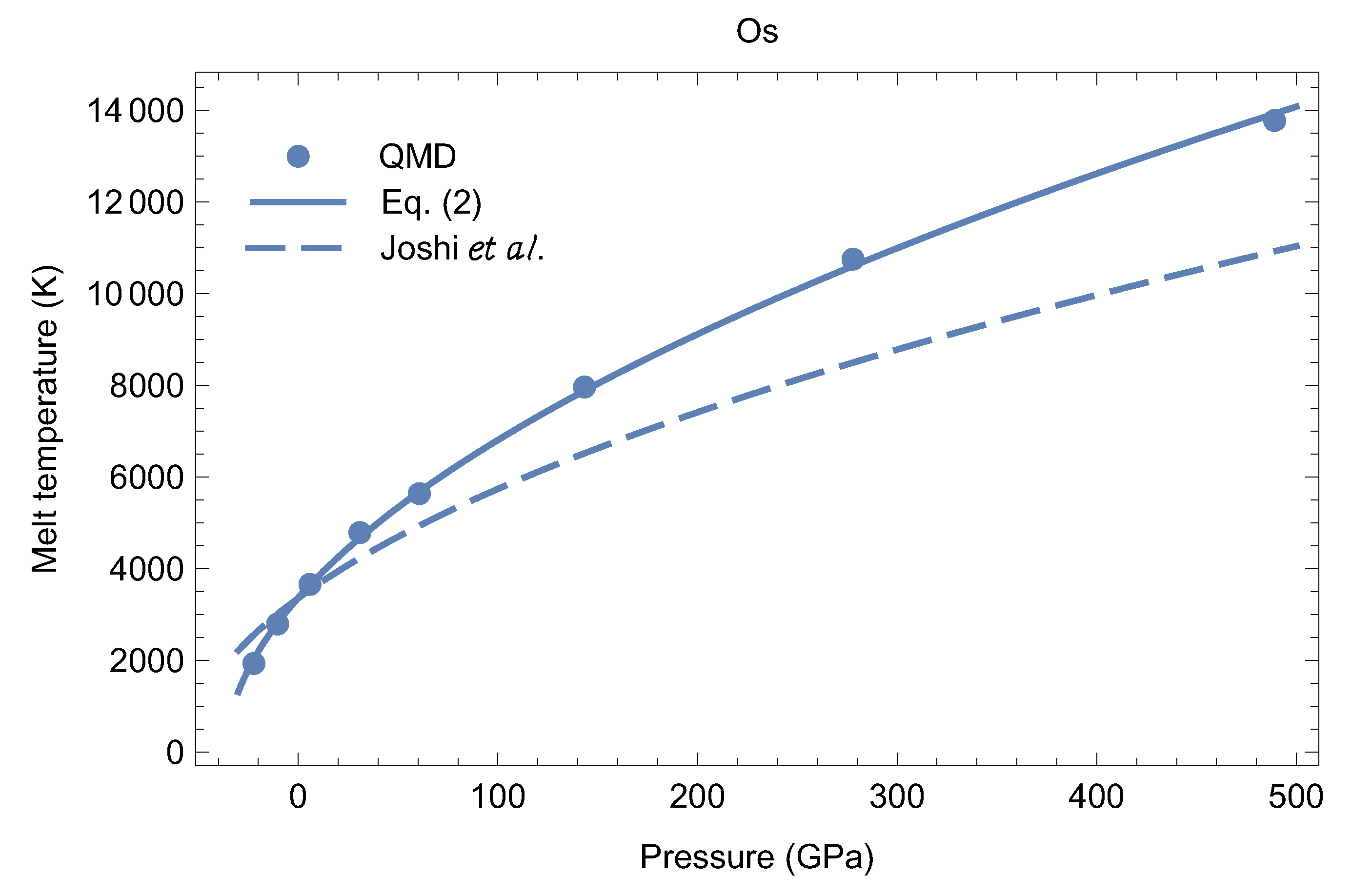
An analytic expression for the melting curve of Os in the P-T plane can be constructed as the best fit of the Simon form, $T_m\left(P\right)=T_m\left(0\right){(1+P/a)}^b,$ to all eight QMD points with $T_m\left(0\right)=3370$ K. The result is (T in K, P in GPa)

$$T_m\left(P\right)=3370{\left(1+\frac{P}{36.1}\right)}^{0.53}.$$

(2)

The melting curve (2) is shown in Figure 8 along with the eight QMD melting points and the theoretical melting curve of Ref. [17]. The (only) reason for a difference between our melting curve and the one from [17] is most likely the calculation of the Grüneisen $\gamma \left(\rho \right),$ which the latter is based on, not being accurate enough. For (2), $d{T}_m\left(P\right)/dP=49.5$ K/GPa at $P=0,$ in good agreement with the values from [8,9,10,21].

4. Uncertainties in the Values of $T_m$ and $P_m$

We now estimate the uncertainties in the melting temperature and pressure for the computational procedure outlined above.

First of all, changes in P are typically much smaller than that in $T.$ For instance, as seen in Figure 4, Figure 5, Figure 6 and Figure 7, which typify T and P changes during simulated melting, the pressure changes by less than 10% while $\Delta$T∼ 20–25%. We estimate the errors in P to range from a few GPa at low pressures to ∼10 GPa at the highest pressure considered; such errors do not exceed the size of the points in Figure 8. As a reasonable approximation, we can ignore errors in P.

The error in the melting temperature is due to the uncertainty in the maximum temperature for which the Os remains a superheated solid, i.e., the temperature at vertex C in Figure 1. Assume that the melting occurs from a superheated solid state C${}^{{}^{\prime }}$ which lies on the continuation of segment BC in Figure 1 beyond point C; the temperature at C is $T_{SH}$ and that at C${}^{{}^{\prime }}$ is $T_{SH}+\Delta T_{SH}$. Melting from C takes the system to point D at temperature $T_m$, while melting from C${}^{{}^{\prime }}$ leaves the system in a liquid state D${}^{{}^{\prime }}$ on segment DE at temperature $T_m+\Delta T_m$. Following [36], we now consider energy balance for the virtual transitions B→C and B→D${}_{liq}$. The energy increase for B→C is $C_{VS}\left(T_{SH}-T_m^{\left(B\right)}\right)$, where $C_{VS}$ is the solid heat capacity at constant volume and $T_m^{\left(B\right)}$ is the melting temperature at B. The transition B→D${}_{liq}$ can be decomposed into B→D${}_{sol}$ with energy change $C_{VS}\left(T_m-T_m^{\left(B\right)}\right)$, and then melting at D with an energy increase of $T_m\Delta S_m$, where $\Delta S_m$ is the entropy of melting; thus the total energy change for B→D${}_{liq}$ is $C_{VS}\left(T_m-T_m^{\left(B\right)}\right)+T_m\Delta S_m$. Since points C and D${}_{liq}$ have the same energy, we can equate the energy changes for B→C and B→D${}_{liq}$ ($T_m^{\left(B\right)}$ drops out):

$$C_{VS}\left(T_{SH}-T_m\right)=T_m\Delta S_m.$$

(3)

Similarly, for B→C${}^{{}^{\prime }}$ and B→D${}^{{}^{\prime }}$ we have

$$C_{VS}\left(T_{SH}+\Delta T_{SH}-T_m\right)=T_m\Delta S_m+C_{VL}\Delta T_m.$$

(4)

Here $C_{VL}$ is the liquid heat capacity at constant volume. It then follows from (1) and (2) that

$$\Delta T_m=\frac{C_{VS}}{C_{VL}}\Delta T_{SH}.$$

(5)

In the vicinity of the melting point the solid and liquid heat capacities are known to be approximately equal [37,38], hence

$$\Delta T_m\approx \Delta T_{SH}.$$

(6)

We have the simple result that the error in $T_m$ is approximately equal to the difference in the temperatures for the first run during which melting occurs and the true melting run.

The temperature difference between two solid states on segment AC in Figure 1 is about half of the difference of the initial temperatures in the QMD runs. This is so because during a QMD run the initial thermal energy, which is the total system energy, is divided almost equally into potential and kinetic energies, and the latter is the thermal energy of the final state. Therefore, $\Delta T_{SH}$ cannot exceed one half of the difference of the initial temperatures for the first run during which the system melts and the last run during which the system remains superheated. For the present Os calculations, this implies a maximum error of ∼75 K for the first three points on the ab initio melting curve and ∼125 K for the remaining five points. All these errors are less than the size of the corresponding symbols in Figure 8.

5. QMD Simulations of the EOS and the Phase Diagram of Re

We now determine the phase diagram of Re to ∼350 GPa using the Z methodology, which is described in detail in [2,14]. In addition to the Z method described above it consists in the so-called inverse Z method, that is, the solidification of a liquid into a crystalline structure. The inverse Z method allows one to find solid-solid transition boundaries, by solidifying liquid into different solid structures on both sides of the boundary and thereby bracketing its location on the P-T plane.

Our Z methodology calculations were carried out using VASP. We again used the GGA approximation with the PBE exchange-correlation functional. We modeled Re using the electron core-valence representation [${}^{48}$Cd $4f^{14}]5p^{6}5d^{5}6s^2$, i.e., we assigned the 13 outermost electrons of Re to the valence. The valence electrons were represented with a plane-wave basis set with a cutoff energy of 400 eV, while the core electrons were represented by PAW pseudopotentials.

5.1. T = 0 Isotherm

We first calculated the $T=0$ isotherm of Re. Just like for Os, this was done by optimizing the value of $c/a$, i.e., determining the $c/a$ that minimizes the energy at a fixed volume of a hexagonal supercell, and extracting the corresponding value of P. We used a $7\times 7\times 6$ (588-atom) supercell with a single $\mathsf{\Gamma }$-point. With such a large supercell, energy convergence to $\stackrel{<}{\sim }$4.5 meV/atom is achieved, which was verified by performing short runs with $2\times 2\times 2,$ $3\times 3\times 3$, and $4\times 4\times 4$ k-point meshes and comparing their output with that of the 588-atom run with a single $\mathsf{\Gamma }$-point. This introduces additional uncertainty of ∼50 K for the numerical values of $T_m$ which is small compared to uncertainites of the Z method itself (250 K for Re, see below).

In the ab initio approach, the density of Re at $(P,T)=(0,0)$ is 20.686 g/cc, whereas the experimental value is 21.12 g/cc [4]. Alternatively, with VASP, the experimental $(P,T)=(0,0)$ density of 21.12 g/cc corresponds to $(P,T)=(8.2$ GPa, $0)$. Just like for Os, this 2.1% density mismatch, or 8.2 GPa pressure mismatch, is due to the PBE implementation of DFT in our VASP simulations. In order to directly compare our QMD results to experiment, we will apply the 2.1% density correction (8.2 GPa pressure correction) to all VASP results in the $\rho$-T (P-T) plane. Specifically, we will multiply VASP densities by 1.021, or subtract 8.2 GPa from VASP pressures, whichever is relevant.

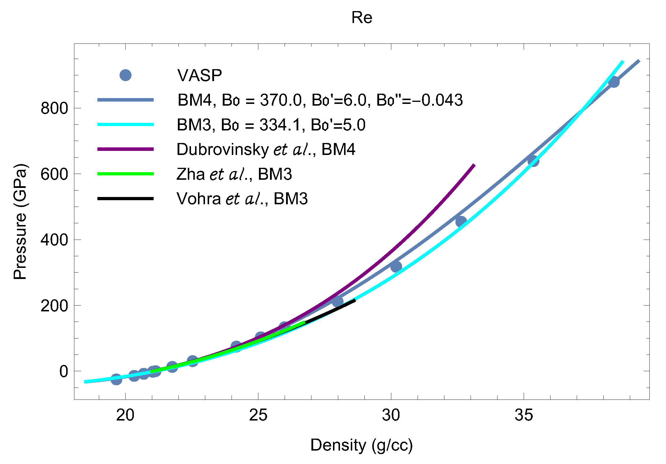
Since the $P=0$ values of the density of Re at $T=0$ and 300 K differ by ∼0.5% (21.12 g/cc vs. 21.02 g/cc [4]), and there is a negligibly small thermal pressure correction at $T=300$ K, the $T=0$ isotherm is a very good approximation to the $T=300$ K isotherm. In Figure 9 we compare room-T isotherm data to our $T=0$ isotherm as determined from QMD; the experimental data are from [3,4,39,40,41]. It is seen that all of the available data and the QMD points are in excellent agreement up to $\rho$∼26 g/cc (P∼150 GPa) beyond which the different sources of data begin to depart from one another. We note that our QMD results are very accurately represented by a fourth-order Birch-Murnaghan EOS (BM4)

$$\begin{array}{c}P\left(\rho \right)=\frac{3}{2}{B}_0\left({\left(\frac{\rho }{{\rho }_0}\right)}^{7/3}-{\left(\frac{\rho }{{\rho }_0}\right)}^{5/3}\right)\left[1+\frac{3}{4}(B_0^{\prime }-4)\left({\left(\frac{\rho }{{\rho }_0}\right)}^{2/3}-1\right)\right.\\ \left.+\frac{3}{8}\left(\frac{143}{9}+(B_0^{\prime }-7)B_0^{\prime }+B_0{B}_0^{″}\right){\left({\left(\frac{\rho }{{\rho }_0}\right)}^{2/3}-1\right)}^2\right],\end{array}$$

(7)

where $B_0,$ $B_0^{\prime }$ and $B_0^{″}$ are the values of the bulk modulus and its first and second pressure derivatives at the reference point $\rho ={\rho }_0$. For practical purposes BM3 (1) can be used as well if $B_0^{\prime }$ is changed from 6 to 5 (see Figure 9).

5.2. c/a Ratio as a Function of P

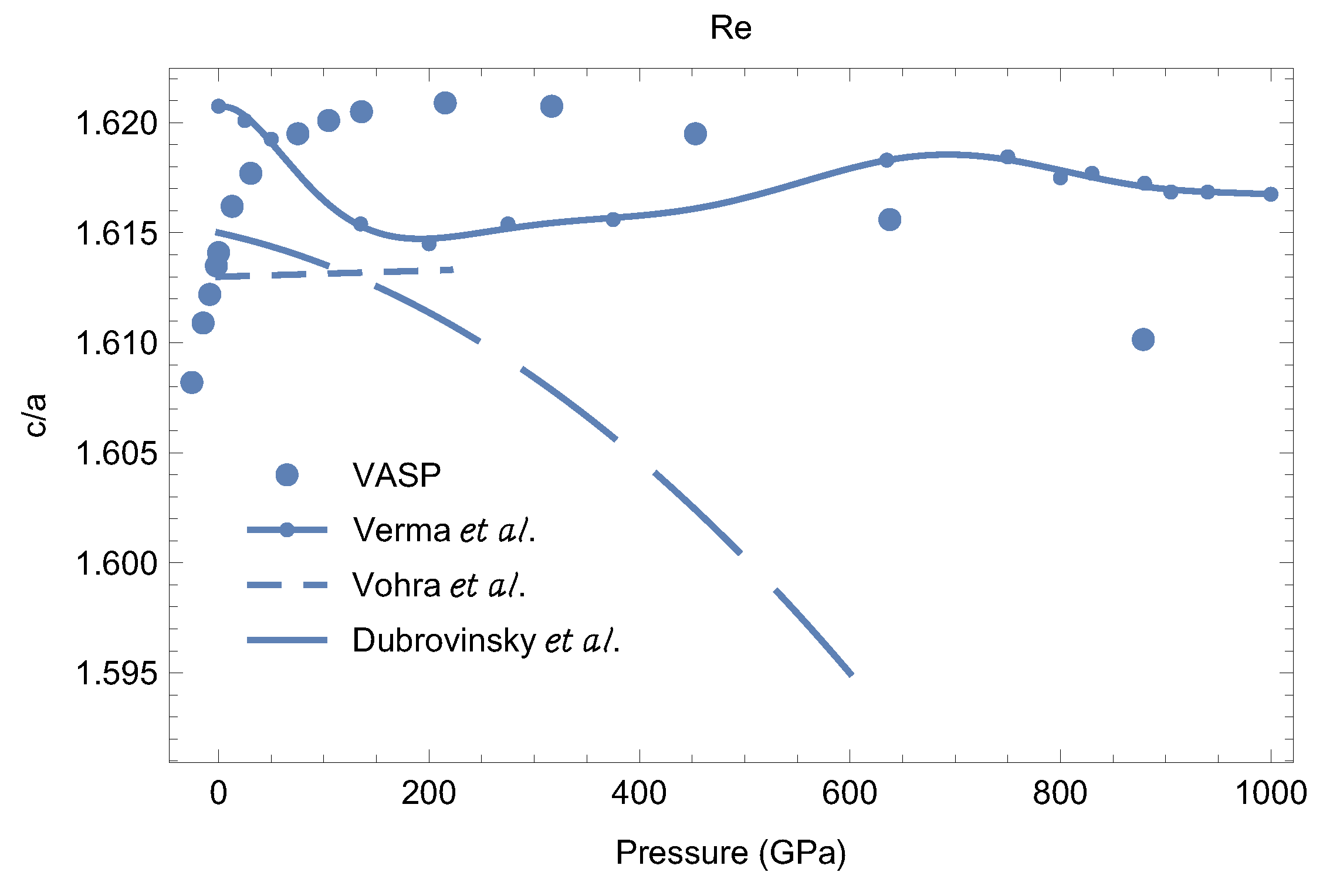
Our results for $c/a$ as a function of P are shown in Figure 10. We find that our theoretical $c/a$ lies in the range $1.615\pm 0.006$ for $P\in [0,900$ GPa] (so that its variation is less than 1%), consistent with experimental data [3,39]. Other theoretical data from [5] have $c/a$ lie in the narrower range of $1.6175\pm 0.003$ (Figure 10) but exhibit quite irregular behavior as a function of $P.$ Our $c/a$ exhibits a P-dependence consistent with that from [3]. Although our calculations demonstrate that hcp-Re remains the most thermodynamically stable solid phase up to at least 900 GPa, in agreement with [5] (a somewhat more detailed discussion will follow), the decreasing $c/a$ may signal its dynamic instability, and the corresponding s-s phase transition, at higher $P.$

5.3. Melting Curve

We then calculated the melting curves of both hcp- and fcc-Re. For fcc-Re, we also used a 588-atom supercell in a hexagonal setting: 3 atoms per unit cell with ABC stacking (the hcp counterpart has 2 atoms per unit cell with AB stacking); the supercell dimension was $7\times 7\times 4.$ By using supercells with the same number of atoms we could make direct comparisons of the hcp and fcc free energies.

We simulated 11 melting points: 6 for hcp-Re and 5 for fcc-Re. At a given density we performed a sequence of long runs, each of 7500–10,500 time steps or 7.5–10.5 ps, with initial temperatures separated by increments of 500 K. We performed 10 QMD runs for each of the 11 melting points; our simulations covered a range of initial T of 4500 K in each case. We carried out a total of 110 runs which, with an average of ∼9000 time steps per run, amounted to a total of ∼1 million time steps for our melting simulations.

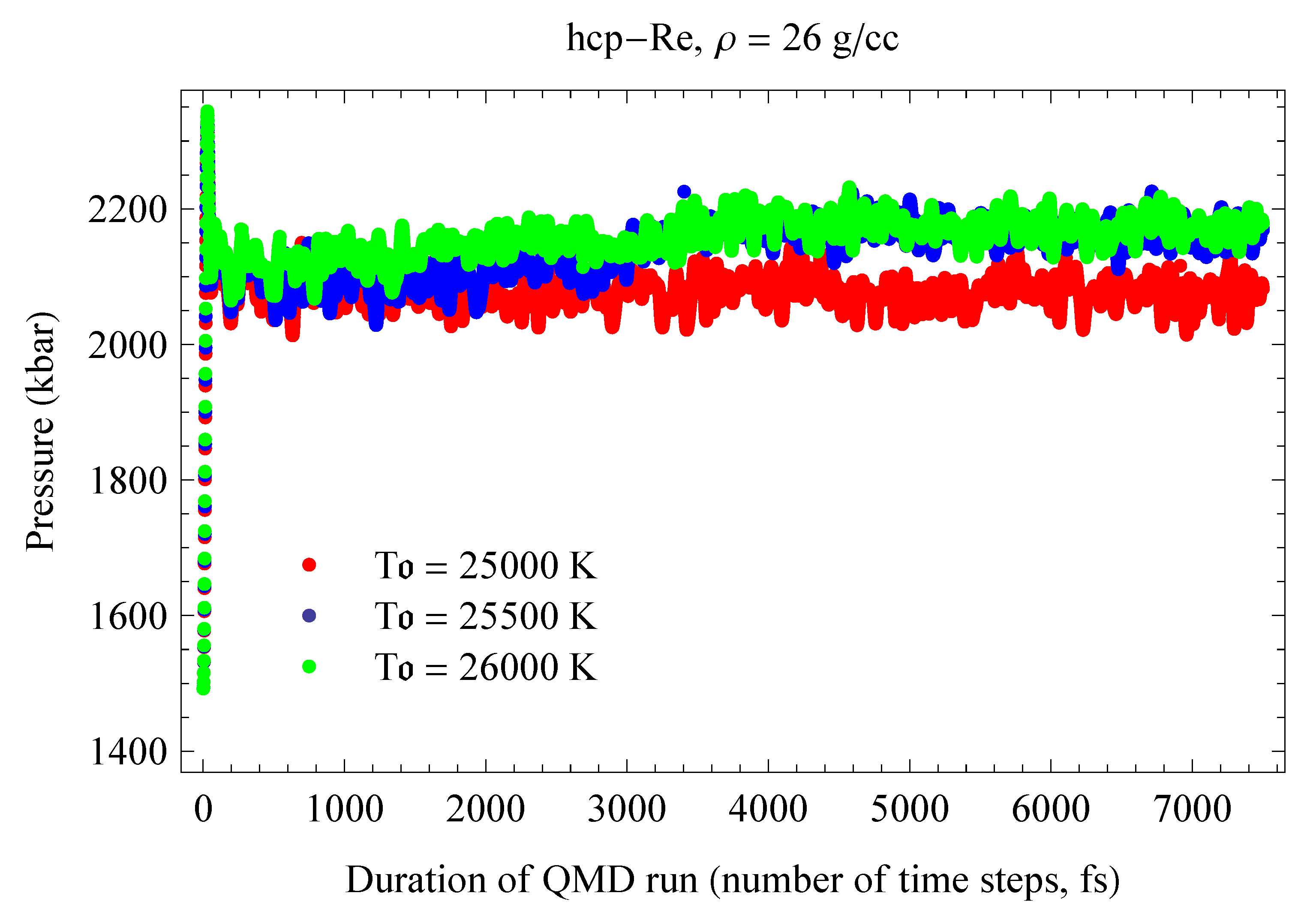
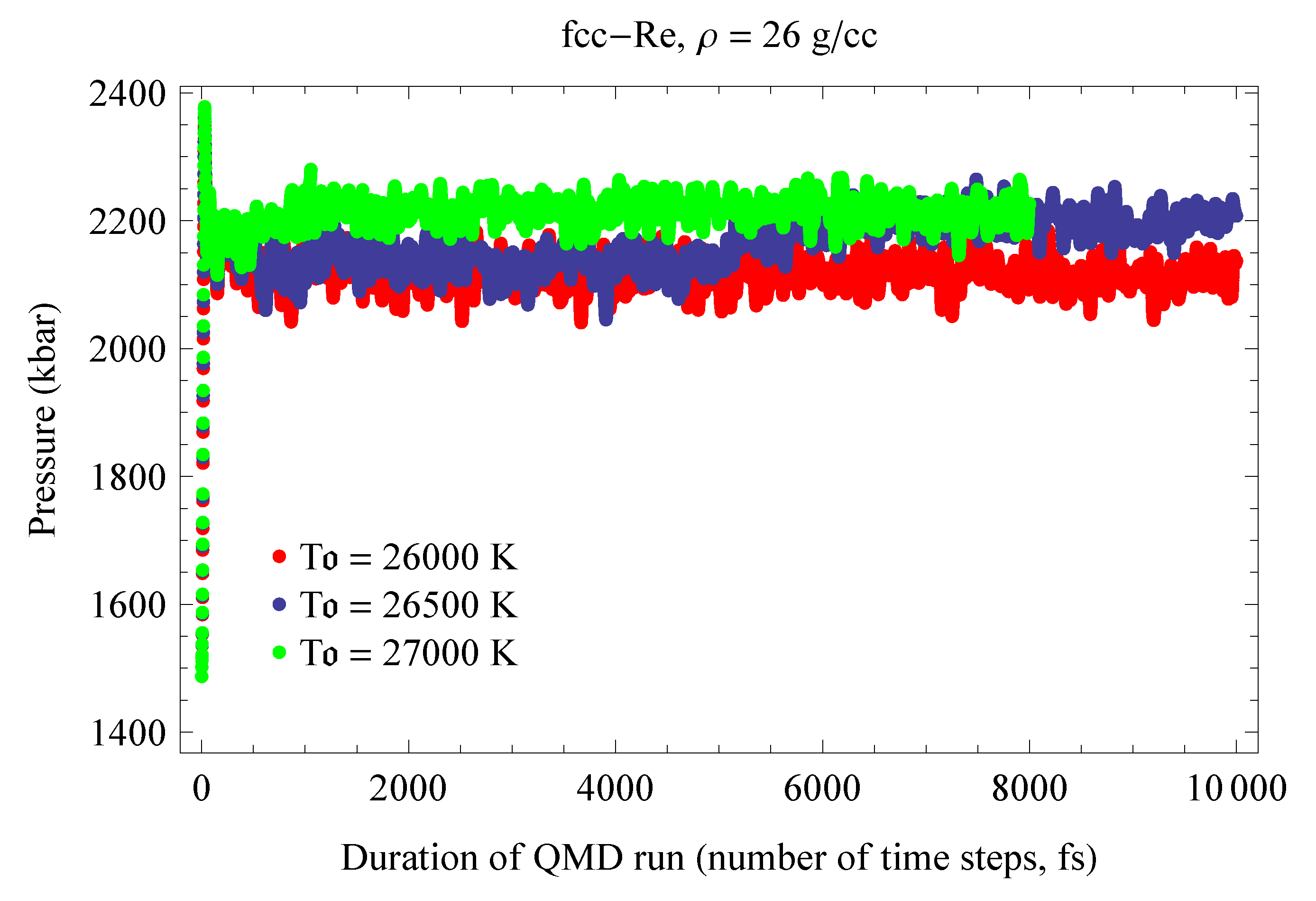
Figure 4 and Figure 5 illustrate the T- and P-evolution of hcp-Re runs with initial temperatures of 25,500, 26,000 and 26,500 K; these runs correspond to the ab initio hcp-Re melting point at ∼209 GPa shown in Figure 11 as an open blue circle. Similarly, Figure 9 and Figure 10 illustrate the T- and P-evolution of the fcc-Re runs that correspond to its ∼212 GPa ab initio melting point shown in Figure 11 as an open green circle.

The 11 melting points of Re are shown in Figure 11. We note that their T error bars are half of the T increment, i.e., $\pm 250$ K, basically the size of the points in Figure 11; the P error bars are very small which we ignore, just like for Os. The melting curve of hcp-Re, as the best fit to the corresponding 6 QMD points, is given by ($T_m$ in K, P in GPa)

$$T_m^{\mathrm{hcp}}\left(P\right)=3460{\left(1+P/58.5\right)}^{0.69},$$

(8)

for which the initial slope is 40.8 K/GPa, in excellent agreement with the VF melting curve obtained by electrical heating [7]. The melting curve of fcc-Re, as the best fit to the corresponding 5 QMD points, is

$$T_m^{\mathrm{fcc}}\left(P\right)=2466{\left(1+P/7.6\right)}^{0.42}.$$

(9)

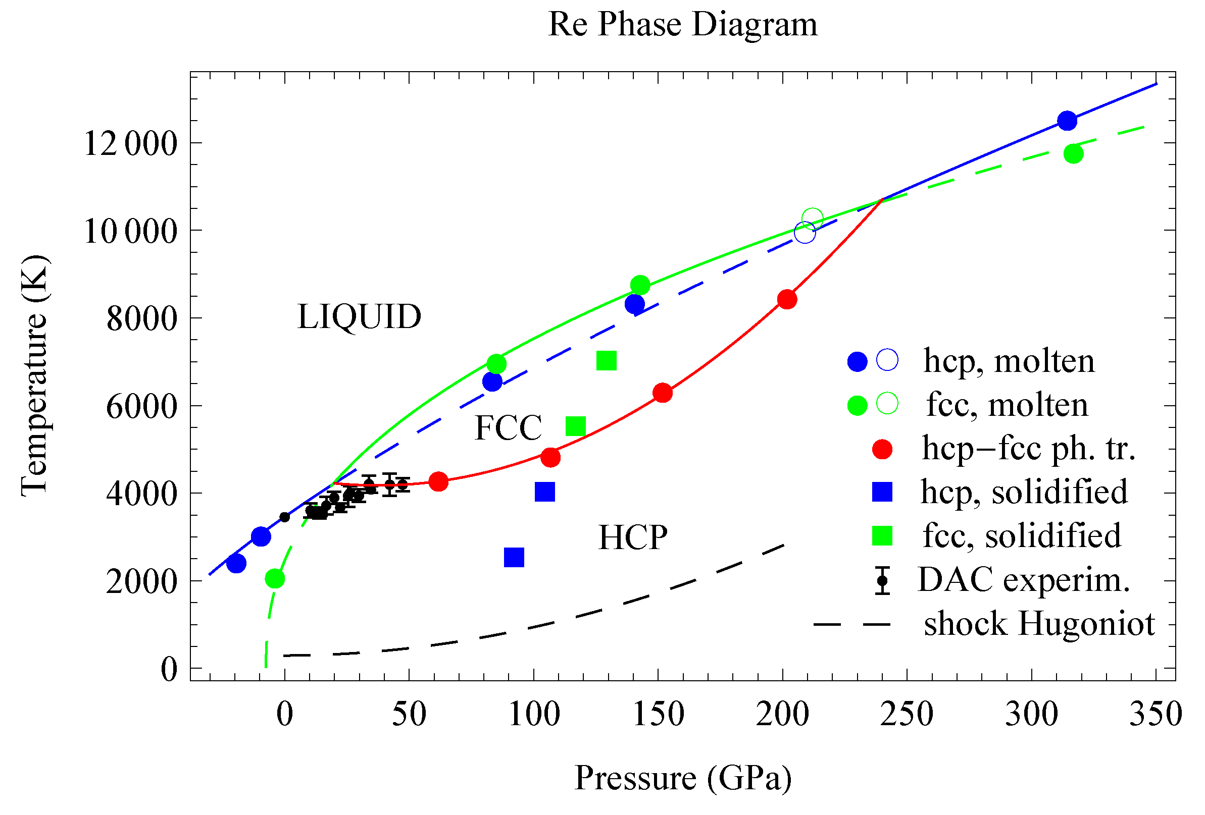
The two melting curves cross each other at (20 GPa, 4240 K) and (240 GPa, 10,650 K), therefore Re melts from fcc over the pressure range 20–240 GPa. In order to determine the exact locaton of the hcp-fcc phase boundary, we carried out full free energy calculations on the two solid structures.

5.4. Full Free Energy Calculations on hcp-Re and fcc-Re

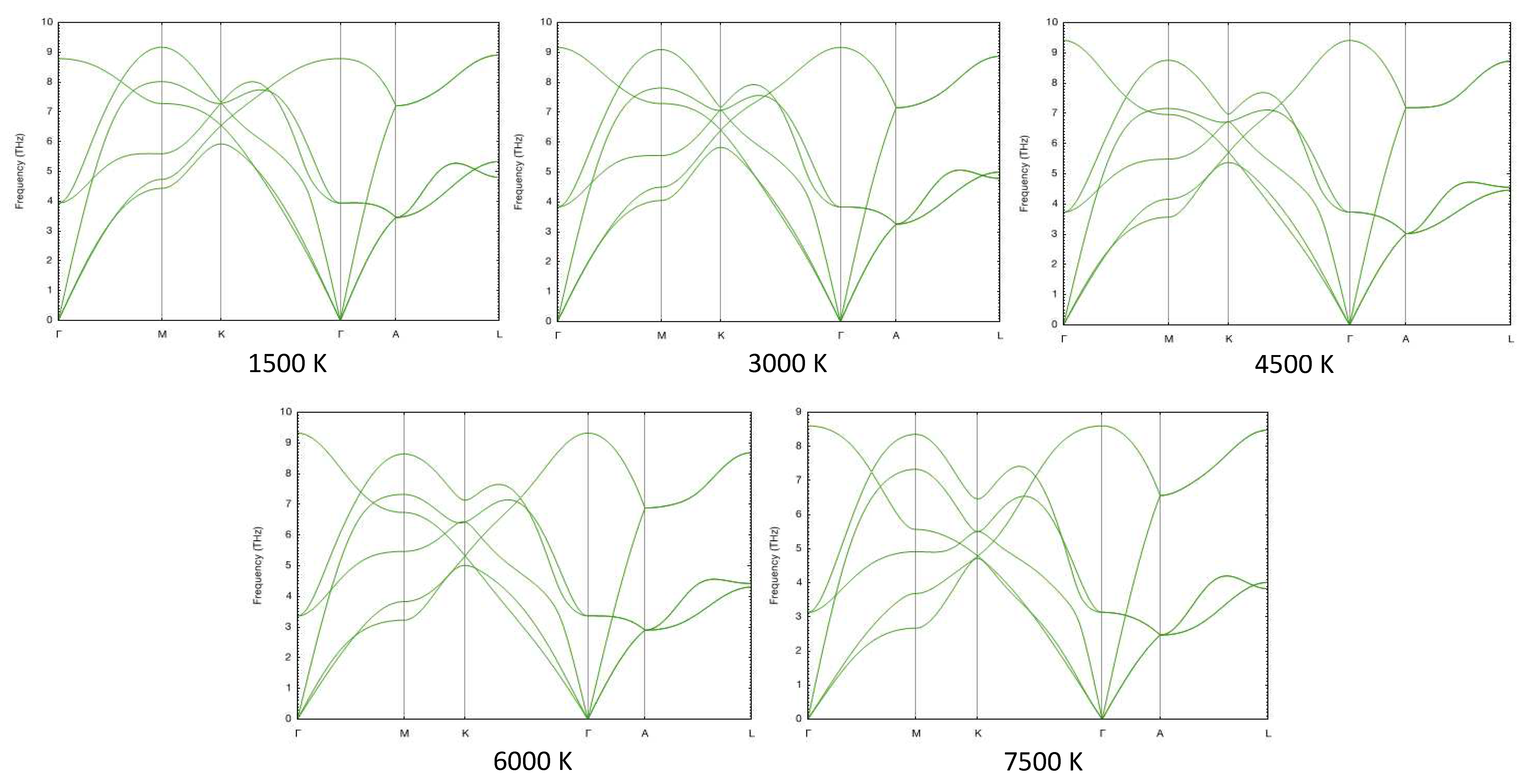
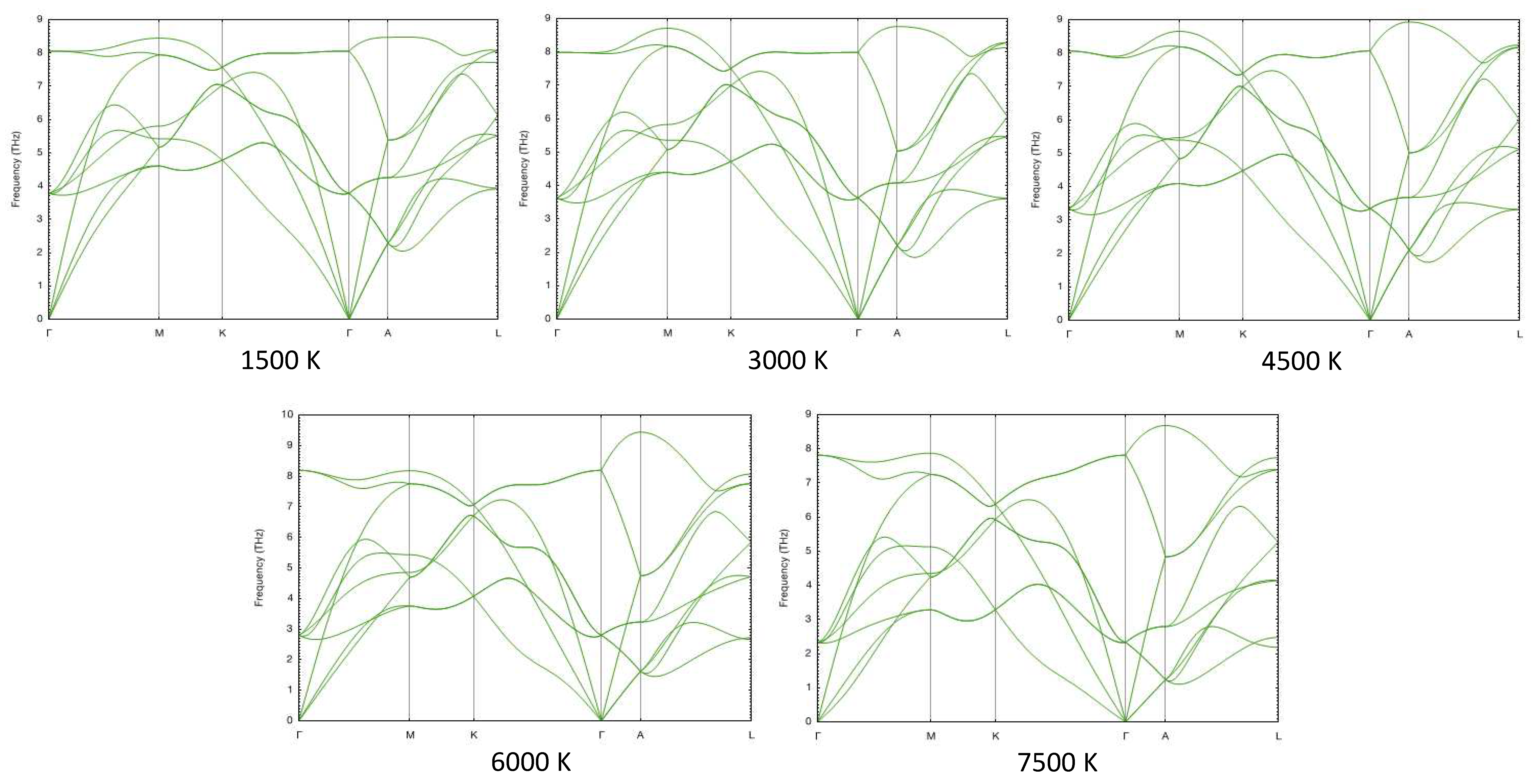
In Figure 12 and Figure 13 we show the phonon spectra of hcp- and fcc-Re, respectively, at one fixed density, namely, 25.1 g/cc (P∼ 115 GPa), at five different temperatures calculated using the temperature-dependent effective potential (TDEP) method [42,43], which takes into account anharmonic lattice vibrations. It is seen that fcc-Re is dynamically stable (no imaginary phonon branches) at all temperatures, and the T-dependence of its phonon spectra is weak. Similar calculations show that fcc-Re is dynamically stable in the whole range of densities considered in this work.

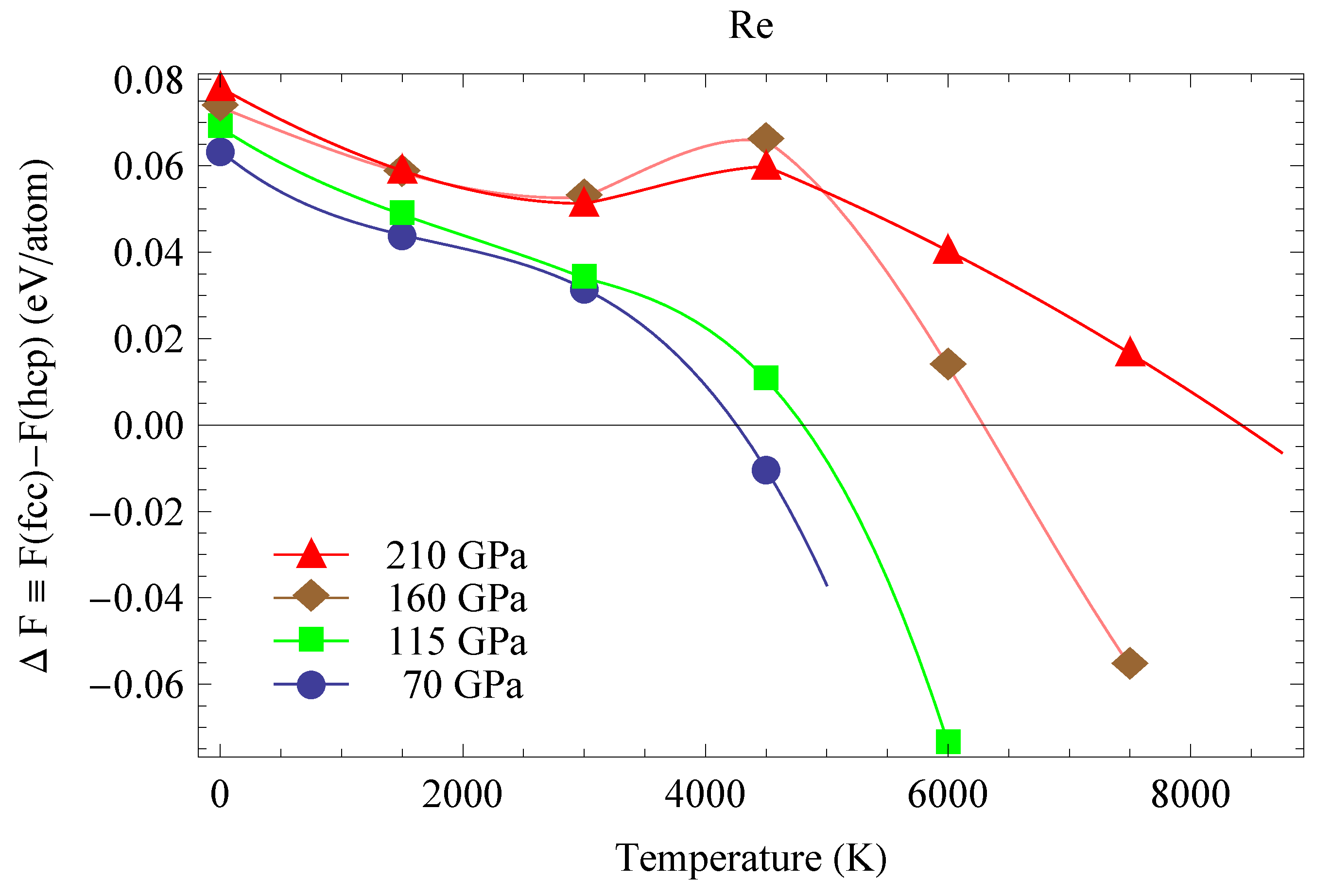
We calculated the full free energies of both fcc-Re and hcp-Re using TDEP. The differences between the full free energies of fcc- and hcp-Re as functions of T at four pressures are shown in Figure 14. The $T=0$ differences between the enthalpies of fcc- and hcp-Re are in excellent agreement with previous calculations (on both hcp-fcc and hcp-bcc free energy differences) [5]; they are the starting points of the four curves in Figure 14. There are four hcp-fcc transition points ($\Delta F=0$). The best fit to these four transition points is $T\left(P\right)=4415-11.9P+0.158P^2$ ($T_m$ in K, P in GPa); this fit is plotted in Figure 11 as a red curve. It crosses the hcp and fcc melting curves at the $(P,T)$ points (20, 4240) and (240, 10,650), which are hcp-fcc-liquid triple points.

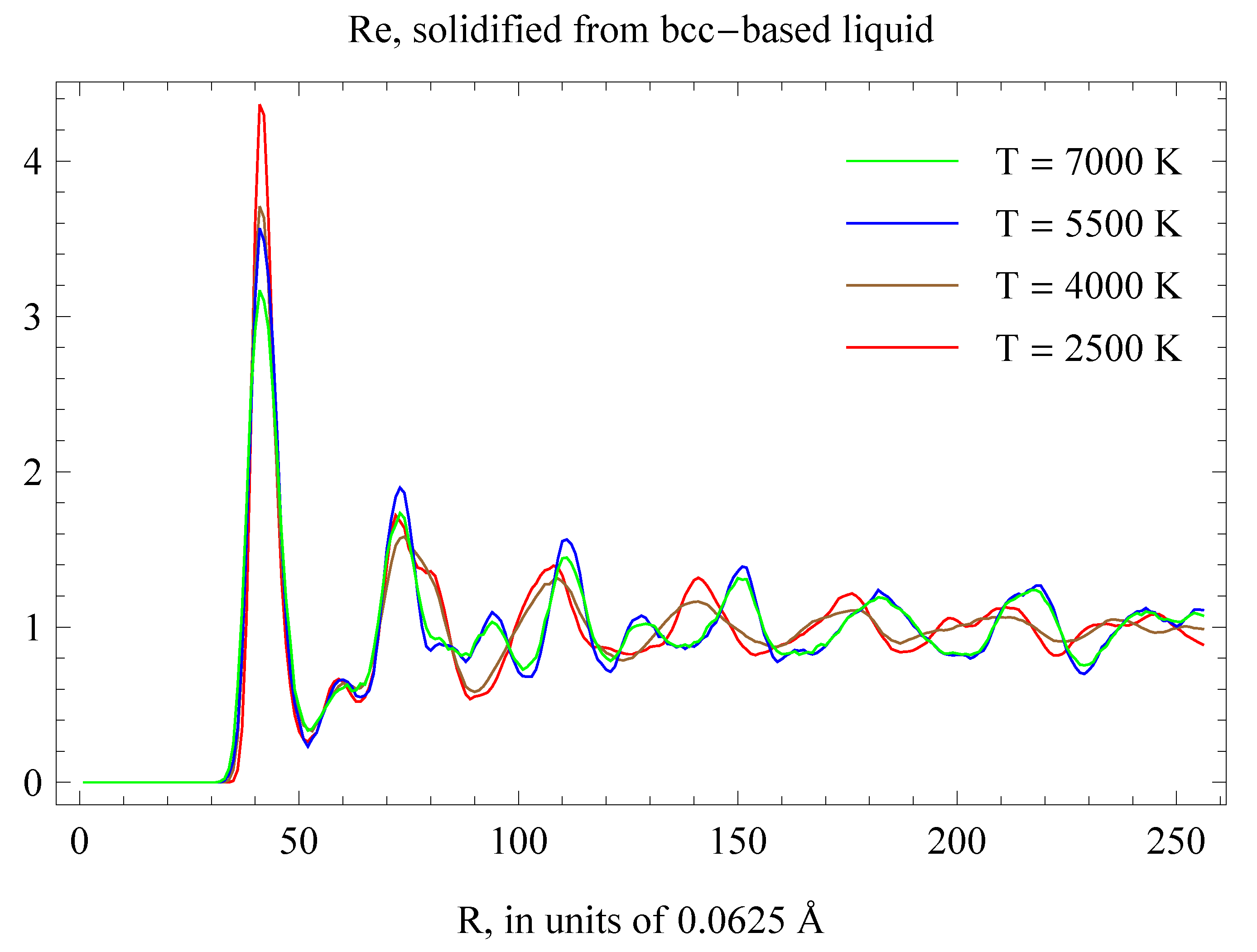
In order to validate the location of the hcp-fcc s-s phase boundary we also carried out a set of four independent inverse Z runs [2] to solidify liquid Re into hcp below the boundary and fcc above it. We used a computational cell of 686 atoms prepared by melting a $7\times 7\times 7$ solid body-centered cubic (bcc) supercell which would eliminate any bias towards solidification into either hcp or fcc. We carried out $NVT$ simulations using the Nosé-Hoover thermostat with a timestep of 1 fs. Complete solidification typically required from 15 to 25 ps, or 15,000–25,000 timesteps. The inverse Z runs indicate that Re does solidify into hcp below the red curve in Figure 11, while above this curve it solidifies into fcc. The radial distribution functions (RDFs) of the final solid states are noisy; upon fast quenching of the four structures to low $T,$ where RDFs are more discriminating, we clearly observed both hcp and fcc; see Figure 15.

Figure 11 also shows the Re principal Hugoniot [44], $T\left(P\right)=293+0.08P^{1.955}$, which crosses the melting curve at (525 GPa, 16,920 K); this is our prediction for the Re melting point in a SW experiment.

5.5. Topological Equivalence of the Phase Diagrams of Re and Pt

We note the topological equivalence of the phase diagrams of Re calculated in this work and that of Pt from our earlier study [2]. In both cases there is a second solid phase—fcc for Re and random hcp (rhcp) for Pt—along the melting curve over a limited range of pressures. The P intervals for the second phase are similar: 20–240 GPa for Re and 35–300 GPa for Pt. The $T=0$ free energy differences between the high-$PT$ and ambient structures grow with P in a similar way: $55+0.11P$ meV/atom for Re and $60+0.07P$ meV/atom for Pt (Supplementary Materials of Ref. [1]). At the corresponding transition points the $T=0$ free energy differences are nearly equal: 57.2 meV/atom for Re vs. 62.5 meV/atom for Pt at the lower-P transition points, and 81.4 meV/atom for Re vs. 81.0 meV/atom for Pt at the upper-P points. Both DAC melting curves are also similar: in both cases the slope of the DAC melting curve is 2.3 times smaller than the actual one (in K/GPa): 17 [6] vs. 40 [7] for Re, and 19.3 [45] vs. 43.8 [2] for Pt. Our results suggest that the DAC melting curve in Figure 11 can be split into two different segments, just like the one for Pt [2]. The first, which lies between the origin and the triple point, is consistent with the ab initio melting curve after taking the DAC error bars into account, and the second segment is above the triple point on the hcp-fcc s-s phase boundary. Fitting a single linear form to these two segments results in a much lower Clapeyron slope for the DAC melting curve, which is apparently the case for both Re and Pt.

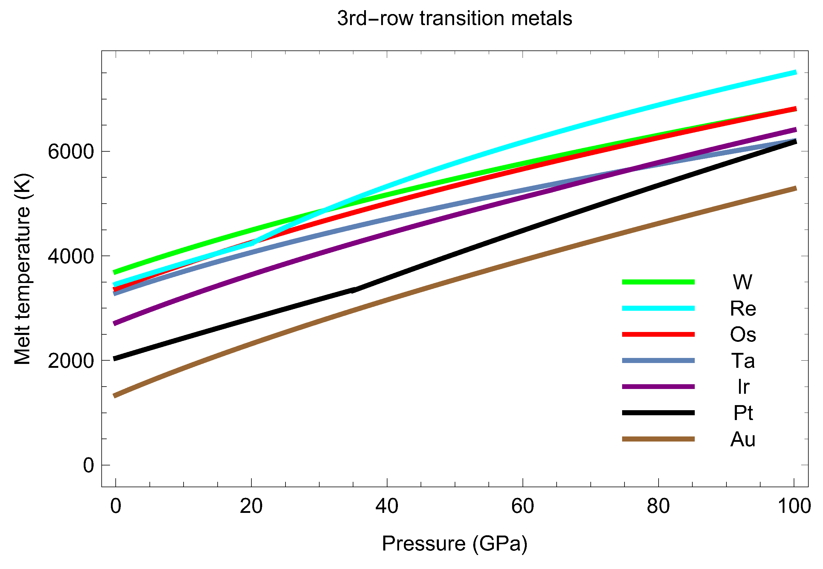
6. 3rd-Row Transition Metal Melting Systematics

Of all the 3rd-row transition metals, only the melting curve of Hf has never been measured or calculated yet. In addition to the melting curves of Re and Os calculated in this work, in Figure 16 we also plot the melting curves of Ta [15,23], W [16], Ir [14], Pt [2,25,28], and Au [11,12,13]. As seen in Figure 16, all the seven 3rd-row transition metal melting curves have low curvature and comparable slopes, roughly 45 K/GPa. These regularities form the 3rd-row transition metal melting systematics. The initial slopes of the seven melting curves can be grouped accoring to (i) crystal structure, (ii) relative location in the periodic table (PT), and (iii) topological equivalence of the phase diagrams (for Re and Pt). More specifically, these initial slopes are (in K/GPa): ∼55 for Au, ∼50 for Os and Ir (PT neighbors that have very similar mechanical and bulk properties, mass density in particular; although their ambient crystal structures are different, fcc iridium transforms into hexagonal structure at high-$PT$ [14]), ∼45 for W and Ta (PT neighbors, both bcc), and ∼40 for Re and Pt (that have topologically equivalent phase diagrams albeit different ambient crystal structures). Even the numerical values of the parameters $(a,b)$ in the Simon form of the melting curve, $T_m=T_m\left(0\right){(1+P/a)}^b,$ can be grouped accordingly: $(36.1,0.53)$ for Os and $(31.2,0.59)$ for Ir, and $(35.1,0.47)$ for Ta and $(41.8,0.5)$ for W. The exception is the pair Re and Pt for which the corresponding sets are somewhat different: $(58.5,0.69)$ for Re and $(44.3,0.85)$ for Pt. We now demonstrate how this melting systematics combined with the $P=0$ value of the melting temperature can be used to estimate the currently unknown melting curve of the 8th 3rd-row transition metal Hf.

Hf Melting Curve Estimate

At ambient P Hf is a hcp metal; on increasing T it undergoes a hcp-bcc structural transformation at ∼2000 K and then melts (from bcc) at 2506 K [46]. To estimate the numerical values of the parameters $(a,b)$ in the Simon form of its melting curve, $T_m=T_m\left(0\right){(1+P/a)}^b,$ we refer to its 3rd-row bcc counterparts Ta and W for which the corresponding values are given above. Since the values of b are close to each other, and all three are PT neighbors with $Z=$72, 73, and 74, the value of b for Hf should be close to those for Ta and W. If there is any Z dependence of $b,$ perhaps it may be approximated by a linear function over a short Z interval (72–74) to yield $b\left(72\right)\approx 0.44.$ We therefore assume that for Hf $b=0.47\pm 0.03,$ which seems to encompass all the possibilities. As regards $a,$ a linear extrapolation of the corresponding Ta and W values would give 28.4 for Hf, but $a=35.1\pm 6.7$ (to cover all possible values from 28.4 to tungsten’s 41.8) will produce a large uncertainty in the corresponding values of $T_m.$ We assume that a for Hf is not larger than that for Ta (35.1) but its error is essentially smaller than 6.7$(=(41.8-28.4)/2);$ speficially, we choose $a=32.5\pm 2.5.$ Thus, our estimate for the melting curve of Hf is

$$T_m\left(P\right)=2506{\left(1+\frac{P}{32.5\pm 2.5}\right)}^{0.47\pm 0.03}.$$

(10)

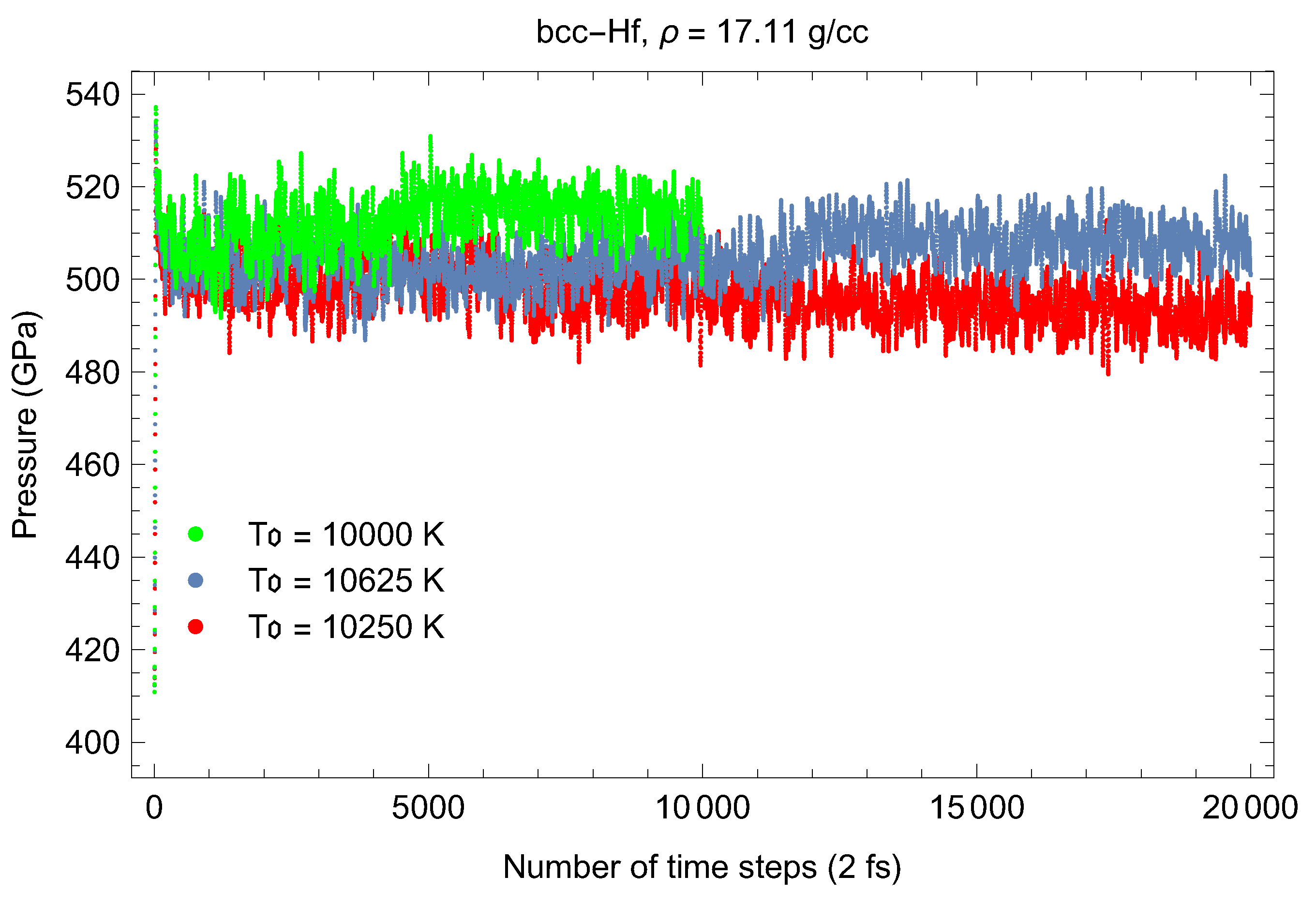
In order to test this estimate, we carried out the calculation of two melting points of Hf using the Z method implemented with VASP. We ran bcc-Hf cells of 432 atoms $(6\times 6\times 6),$ having lattice constants of 3.26 Å and 2.65 Å, or densities of 17.11 g/cc and 31.85 g/cc, which correspond to ∼50 and 500 GPa, respectively, with a single $\mathsf{\Gamma }$ point. We chose a timestep of 2 fs and an initial T increment of 375 K (so that the $T_m$ error is roughly $\pm 200$ K) in each case. Figure 17 and Figure 18 show the time evolution of T and P in the sets of runs that include the melting run, in one of these cases, namely, $\rho =17.11$ g/cc. Our simulated $(P,T)$ melting points are (T in K, P in GPa) $(51,3940)$ and $(497,9465).$ The corresponding values of T from (10) are $3905\pm 140$ and $9303\pm 840,$ in excellent agreement with our VASP results. Thus, our estimate (10) is at least a very good approximation for the actual melting curve of Hf over a wide range of $P,$ 0–500 GPa. A more consistent calculation of the melting curve of Hf, which requires simulating additional number of its melting points, goes far beyond the scope of this work; it will be undertaken in one of our future research projects.

7. Concluding Remarks

We have calculated the melting curve of Os using the Z method based on first-principles QMD implemented with VASP. We have also calculated the phase diagram of Re to 350 GPa including the melting temperatures of both hcp-Re and fcc-Re. We have run a total of about 2 million time steps in our QMD simulations on Os, and over 1 million time steps in those on Re; however, the high accuracy of the results and their importance to the field of phase diagram studies justifies the computational cost. Our calculated melting curve of hcp-Re is in excellent agreement with the low-pressure experimental data of VF [7]. Free energy calculations using TDEP and inverse Z simulations yield the same hcp-fcc phase boundary. We have shown that the recent DAC data of YKB [6] in fact map out the hcp-fcc s-s phase boundary. The phase diagram of Re is topologically equivalent to that of Pt. The two DAC melting curves are also similar: in both cases the slope of the DAC melting curve is 2.3 times smaller than the correct one because of fitting a single linear form to its two segments; the first is along the melting curve between the origin and the triple point, and the second is above the triple point along the s-s phase boundary. Our findings suggest that the DAC melting curve may be erroneous in some other cases. In fact, the older low-slope DAC melting curve may map out either the corresponding s-s phase boundary, similar to the cases of Re and Pt, or a solid texture transition line, similar to the case of Mo for which such a texture transition was discovered in the most recent experimental study [47]. The resolution of this issue calls for additional study, both experimental and theoretical. Regularities in the melting curves of Re, Os, and five other 3rd-row transition metals form the 3rd-row transition metal melting systematics. We have demonstrated how this systematics can be used to estimate the currently unknown melting curve of the eighth 3rd-row transition metal Hf.

References

- Dubrovinsky, L.; Dubrovinskaya, N.; Crichton, W.A.; Mikhaylushkin, A.S.; Simak, S.I.; Abrikosov, I.A.; de Almeida, J.S.; Ahuja, R.; Luo, W.; Johansson, B. Noblest of all metals is structurally unstable at high pressure. Phys. Rev. Lett. 2007, 98, 045503. [Google Scholar] [CrossRef] [PubMed]
- Burakovsky, L.; Chen, S.P.; Preston, D.L.; Sheppard, D.G. Z methodology for phase diagram studies: Platinum and tantalum as examples. J. Phys. Conf. Ser. 2014, 500, 162001. [Google Scholar] [CrossRef]
- Dubrovinsky, L.; Dubrovinskaia, N.; Prakapenka, V.B.; Abakumov, A.M. Implementation of micro-ball nanodiamond anvils for high-pressure studies above 6 Mbar. Nat. Commun. 2012, 3, 1163. [Google Scholar] [CrossRef] [PubMed] [Green Version]
- Zha, C.-S.; Bassett, W.A.; Shim, S.-H. Rhenium, an in situ pressure calibrant for internally heated diamond anvil cells. Rev. Sci. Instrum. 2004, 75, 2409–2418. [Google Scholar] [CrossRef]
- Verma, A.K.; Ravindran, P.; Rao, R.S.; Godwal, B.K.; Jeanloz, R. On the stability of rhenium up to 1 TPa pressure against transition to the bcc structure. Bull. Mater. Sci. 2003, 26, 183–187. [Google Scholar] [CrossRef]
- Yang, L.; Karandikar, A.; Boehler, R. Flash heating in the diamond cell: Melting curve of rhenium. Rev. Sci. Instrum. 2012, 83, 063905. [Google Scholar] [CrossRef] [PubMed]
- Vereshchagin, L.F.; Fateeva, N.S. Melting curve of rhenium up to 80 kbar. JETP Lett. 1975, 22, 106. [Google Scholar]
- Regel’, A.R.; Glazov, V.M. Periodicheskiy zakon i fizicheskie svoistva elektronnykh rasplavov. In The Periodic Law and Physical Properties of Electronic Melts; Nauka: Moscow, Russia, 1978. [Google Scholar]
- Gorecki, T. Vacancies and melting curves of metals at high pressure. Zeitschrift für Metallkunde 1977, 68, 231–236. [Google Scholar]
- Gorecki, T. Vacancies and a generalised melting curve of metals. High Temp. High Press. 1979, 11, 683–692. [Google Scholar]
- Decker, D.L.; Vanfleet, H.B. Melting and high-temperature electrical resistance of gold under pressure. Phys. Rev. 1965, 138, A129. [Google Scholar] [CrossRef]
- Tsuchiya, T. First-principles prediction of the P-V-T equation of state of gold and the 660-km discontinuity in Earth’s mantle. J. Geophys. Res. 2003, 108, 2462. [Google Scholar] [CrossRef]
- Pippinger, T.; Dubrovinsky, L.; Glazyrin, K.; Miletich, R.; Dubrovinskaya, N. Detection of melting by in-situ observation of spherical-drop formation in laser-heated diamond-anvil cells. Física de la Tierra 2011, 23, 2011. [Google Scholar]
- Burakovsky, L.; Burakovsky, N.; Cawkwell, M.J.; Preston, D.L.; Errandonea, D.; Simak, S.I. Ab initio phase diagram of iridium. Phys. Rev. B 2016, 94, 094112. [Google Scholar] [CrossRef]
- Dewaele, A.; Mezouar, M.; Guignot, N.; Loubeyre, P. High melting points of tantalum in a laser-heated diamond anvil cell. Phys. Rev. Lett. 2010, 104, 255701. [Google Scholar] [CrossRef] [PubMed]
- Baty, S.R.; Burakovsky, L.; Preston, D.L. Ab initio melting curve of tungsten and W93 alloy. 2018; in preparation. [Google Scholar]
- Joshi, K.D.; Gupta, S.C.; Banerjee, S. Shock Hugoniot of osmium up to 800 GPa from first principles calculations. J. Phys. Condens. Matter 2009, 21, 415402. [Google Scholar] [CrossRef] [PubMed]
- Dubrovinsky, L.; Dubrovinskaya, N.; Bykova, E.; Bykov, M.; Prakapenka, V.; Prescher, C.; Glazyrin, K.; Liermann, H.-P.; Hanfland, M.; Ekholm, M.; et al. The most incompressible metal osmium at static pressures above 750 gigapascals. Nature 2015, 525, 226. [Google Scholar] [CrossRef] [PubMed]
- Godwal, B.K.; Yan, J.; Clark, S.M.; Jeanloz, R. High-pressure behavior of osmium: An analog for iron in Earth’s core. J. Appl. Phys. 2012, 111, 112608. [Google Scholar] [CrossRef]
- Armentrout, M.M.; Kavner, A. Incompressibility of osmium metal at ultrahigh pressures and temperatures. J. Appl. Phys. 2010, 107, 093528. [Google Scholar] [CrossRef]
- Kulyamina, E.Y.; Zitserman, V.Y.; Fokin, L.R. Osmium: Melting curve and matching of high temperature data. High Temp. 2015, 53, 151–154. [Google Scholar] [CrossRef]
- Belonoshko, A.B.; Burakovsky, L.; Chen, S.P.; Johansson, B.; Mikhaylushkin, A.S.; Preston, D.L.; Simak, S.I.; Swift, D.C. Molybdenum at high pressure and temperature: Melting from another solid phase. Phys. Rev. Lett. 2008, 100, 135701. [Google Scholar] [CrossRef] [PubMed]
- Burakovsky, L.; Chen, S.P.; Preston, D.L.; Belonoshko, A.B.; Rosengren, A.; Mikhaylushkin, A.S.; Simak, S.I.; Moriarty, J.A. High-pressure–high-temperature polymorphism in Ta: Resolving an ongoing experimental controversy. Phys. Rev. Lett. 2010, 104, 255702. [Google Scholar] [CrossRef] [PubMed]
- Belonoshko, A.B.; Rosengren, A.; Burakovsky, L.; Preston, D.L.; Johansson, B. Melting of Fe and Fe0.9375Si0.0625 at Earth’s core pressures studied using ab initio molecular dynamics. Phys. Rev. B 2009, 79, 220102. [Google Scholar] [CrossRef]
- Belonoshko, A.B.; Rosengren, A. High-pressure melting curve of platinum from ab initio Z method. Phys. Rev. B 2012, 85, 174104. [Google Scholar] [CrossRef]
- Dewaele, A.; Mezouar, M.; Guignot, N.; Loubeyre, P. Melting of lead under high pressure studied using second-scale time-resolved x-ray diffraction. Phys. Rev. B 2007, 76, 144106. [Google Scholar] [CrossRef]
- Anzellini, S.; Dewaele, A.; Mezouar, M.; Loubeyre, P.; Morard, G. Melting of iron at Earth’s inner core boundary based on fast x-ray diffraction. Science 2013, 340, 464–466. [Google Scholar] [CrossRef] [PubMed]
- Errandonea, D. High-pressure melting curves of the transition metals Cu, Ni, Pd, and Pt. Phys. Rev. B 2013, 87, 054108. [Google Scholar] [CrossRef]
- Arblaster, J.W. Is osmium always the densest metal? A comparison of the densities of iridium and osmium. Johns. Matthey Technol. Rev. 2014, 58, 137–141. [Google Scholar] [CrossRef]
- Arblaster, J.W. Crystallographic properties of osmium. Platin. Metals Rev. 2013, 57, 177–185. [Google Scholar] [CrossRef]
- Occelli, F.; Farber, D.L.; Badro, J.; Aracne, C.M.; Teter, D.M.; Hanfland, M.; Canny, B.; Couzinet, B. Experimental evidence for a high-pressure isostructural phase transition in osmium. Phys. Rev. Lett. 2004, 93, 095502. [Google Scholar] [CrossRef] [PubMed] [Green Version]
- Takemura, K.; Arai, M.; Kobayashi, K.; Sasaki, T. Bulk modulus of Os by experiments and first-principles calculations. In Proceedings of the 20th AIRAPT—43th EHPRG, Karlsruhe, Germany, 27 June 27–1 July 2005; Available online: http://bibliothek.fzk.de/zb/verlagspublikationen/AIRAPT_EHPRG2005/Posters/P139.pdf (accessed on 10 December 2017).
- Kenichi, T. Bulk modulus of osmium: High-pressure powder x-ray diffraction experiments under quasihydrostatic conditions. Phys. Rev. B 2004, 70, 012101. [Google Scholar] [CrossRef]
- Perreault, C.S.; Velisavljevic, N.; Vohra, Y.K. High-pressure structural parameters and equation of state of osmium to 207 GPa. Cogent Phys. 2017, 4, 1376899. [Google Scholar] [CrossRef]
- Sahu, B.R.; Kleimann, L. Osmium is not harder than diamond. Phys. Rev. B 2005, 72, 113106. [Google Scholar] [CrossRef]
- Belonoshko, A.B.; Skorodumova, N.V.; Rosengren, A.; Johansson, B. Melting and critical superheating. Phys. Rev. B 2006, 73, 012201. [Google Scholar] [CrossRef]
- Grover, R. Liquid metal equation of state based on scaling. J. Chem. Phys. 1971, 55, 3435. [Google Scholar] [CrossRef]
- Grover, R. Metallic high pressure equation of state derived from experimental data. In High Pressure Science and Technology, Proceedings of the 6th AIRAPT Conference, Boulder, CO, USA, 25–29 July 1977; Plenum Press: New York, NY, USA, 1979; Volume 1, p. 33, In this paper it is suggested that, for CVL at a given density, CVL = is a good average representation of all the available experimental data and computer simulations on liquid metals, including those for the OCP. Hence, at T = Tm, CVL = . Since CVS ≅ 3R, CVL ≅ CVS ≈ CVS. [Google Scholar]
- Vohra, Y.K.; Duclos, S.J.; Ruoff, A.L. High-pressure x-ray diffraction studies on rhenium up to 216 GPa (2.16 Mbar). Phys. Rev. B 1987, 36, 9790. [Google Scholar] [CrossRef]
- Anzellini, S.; Dewaele, A.; Occelli, F.; Loubeyre, P.; Mezouar, M. Equation of state of rhenium and application for ultra high pressure calibration. J. Appl. Phys. 2014, 115, 043511. [Google Scholar] [CrossRef]
- Jeanloz, R.; Godwal, B.K.; Meade, C. Static strength and equation of state of rhenium at ultra-high pressures. Nature 1991, 349, 687. [Google Scholar] [CrossRef]
- Hellman, O.; Abrikosov, I.A.; Simak, S.I. Lattice dynamics of anharmonic solids from first principles. Phys. Rev. B 2011, 84, 180301. [Google Scholar] [CrossRef]
- Hellman, O.; Steneteg, P.; Abrikosov, I.A.; Simak, S.I. Temperature dependent effective potential method for accurate free energy calculations of solids. Phys. Rev. B 2013, 87, 104111. [Google Scholar] [CrossRef]
- Kinslow, R. (Ed.) High-Velocity Impact Phenomena; Academic Press: New York, NY, USA; London, UK, 1970; p. 544. [Google Scholar]
- Kavner, A.; Jeanloz, R. High-pressure melting curve of platinum. J. Appl. Phys. 1998, 83, 7553–7559. [Google Scholar] [CrossRef]
- Ostanin, S.A.; Trubitsin, V.Y. Calculation of the P-T phase diagram of hafnium. Comput. Mater. Sci. 2000, 17, 174. [Google Scholar] [CrossRef]
- Hrubiak, R.; Meng, Y.; Shen, G. Microstructures define melting of molybdenum at high pressures. Nat. Commun. 2017, 8, 14562. [Google Scholar] [CrossRef] [PubMed] [Green Version]
Figure 1.
Typical isochore used in the Z methodology. Different segments of the isochore correspond to solid (AB), superheated solid (BC), liquid (DE), and supercooled liquid (DF) states. Melting corresponds to segment CD. Isochoric and isothermal solidification processes correspond to segments FB and GH, respectively, and are used in the so-called inverse Z method [2].
Figure 2.
The T = 0 Os EOS from VASP compared to the experimental 300 K 3rd-order Birch-Murnagan (BM3) EOSs from different literature sources [18,31,34]. The pressure ranges of the experimental EOSs are those in which they were measured.
Figure 3.
The ratio as a function of P: QMD vs. the available experimental data from different literature sources [18,31,32].
Figure 4.
Time evolution of T for hcp-Re in three QMD runs with initial temperatures (s) separated by 500 K. The middle run is the melting run, during which T decreases from ∼12,000 K for the superheated state to ∼10,000 K for the liquid at the corresponding melting point.
Figure 5.
The same as in Figure 4 for the time evolution of P. During melting P increases from ∼210 GPa for the superheated state to ∼217 GPa for the liquid at the corresponding melting point.
Figure 6.
The same as in Figure 4 for fcc-Re.
Figure 7.
Figure 8.
The melting curve of Os: VASP results (bullets) and the corresponding Simon equation, Equation (2), vs. the theoretical model of Joshi et al. [17].
Figure 9.
The T = 0 Re EOS from VASP compared to the experimental 300 K EOSs from different literature sources [3,4,39]. The pressure ranges of the experimental EOSs are those in which they were measured.
Figure 10.
The ratio as a function of P: VASP vs. the available experimental data from different literature sources [3,5,39].
Figure 11.
The phase diagram of Re based on the theoretical results of this work vs. the experimental DAC data of Ref. [6].
Figure 12.
Phonon spectra of hcp-Re as functions of T at a fixed density of 25.1 g/cc.
Figure 13.
Phonon spectra of fcc-Re as functions of T at a fixed density of 25.1 g/cc.
Figure 14.
The hcp-Re–fcc-Re full free energy differences as functions of T at four pressures.
Figure 15.
RDFs of the final states in the inverse Z simulations described in the text.
Figure 16.
The melting systematics of the 3rd-row transition metals based on the available experimental and/or theoretical data.
Figure 17.
Time evolution of T for bcc-Hf with a density of 17.11 g/cc in three QMD runs with initial s separated by 375 K.
Figure 18.
The same as in Figure 17 for the time evolution of
© 2018 by the authors. Licensee MDPI, Basel, Switzerland. This article is an open access article distributed under the terms and conditions of the Creative Commons Attribution (CC BY) license (http://creativecommons.org/licenses/by/4.0/).
Share and Cite
MDPI and ACS Style
Burakovsky, L.; Burakovsky, N.; Preston, D.; Simak, S. Systematics of the Third Row Transition Metal Melting: The HCP Metals Rhenium and Osmium. Crystals 2018, 8, 243. https://doi.org/10.3390/cryst8060243
AMA Style
Burakovsky L, Burakovsky N, Preston D, Simak S. Systematics of the Third Row Transition Metal Melting: The HCP Metals Rhenium and Osmium. Crystals. 2018; 8(6):243. https://doi.org/10.3390/cryst8060243
Chicago/Turabian StyleBurakovsky, Leonid, Naftali Burakovsky, Dean Preston, and Sergei Simak. 2018. "Systematics of the Third Row Transition Metal Melting: The HCP Metals Rhenium and Osmium" Crystals 8, no. 6: 243. https://doi.org/10.3390/cryst8060243
Note that from the first issue of 2016, this journal uses article numbers instead of page numbers. See further details here.