Neutron RTOF Stress Diffractometer FSD at the IBR-2 Pulsed Reactor


Frank Laboratory of Neutron Physics, Joint Institute for Nuclear Research, Joliot-Curie Str. 6, 141980 Dubna, Russia
Crystals 2018, 8(8), 318; https://doi.org/10.3390/cryst8080318
Submission received: 18 July 2018
/
Revised: 4 August 2018
/
Accepted: 6 August 2018
/
Published: 9 August 2018
(This article belongs to the Special Issue Neutron Diffractometers for Single Crystals and Powders)
Abstract
:The diffraction of thermal neutrons is a powerful tool for investigations of residual stresses in various structural materials and bulk industrial products due to the non-destructive character of the method and high penetration depth of neutrons. Therefore, for conducting experiments in this research field, the neutron Fourier stress diffractometer FSD has been constructed at the IBR-2 pulsed reactor in FLNP JINR (Dubna, Russia). Using a special correlation technique at the long-pulse neutron source, a high resolution level of the instrument has been achieved (Δd/d ≈ 2 ÷ 4 × 10⁻³) over a wide range of interplanar spacing dhkl at a relatively short flight distance between the chopper and sample position (L = 5.55 m). The FSD design satisfies the requirements of a high luminosity, high resolution, and specific sample environment. In this paper, the current status of the FSD diffractometer is reported and examples of performed experiments are given.
1. Introduction
To investigate internal stresses in materials, various non-destructive methods, including X-ray diffraction, ultrasonic scanning, and a variety of magnetic methods (based on the measurement of magnetic induction, penetrability, anisotropy, Barkhausen effect, and magnetoacoustic effects), have been used for many years. All of them, however, are of limited application. For example, X-ray scattering and magnetic methods can be only used to investigate stresses near surfaces due to their low penetration depth. Besides, the application of magnetic methods is restricted to ferromagnetic materials. In addition, magnetic and ultrasonic methods are greatly influenced by the texture in a sample. The method of mechanical stress investigations by neutron diffraction appeared about 35 years ago. Since then, it has been widely used because of a number of advantages. In contrast to traditional methods, neutrons can non-destructively penetrate into the material to a depth of up to 2–3 cm in steel and up to 5 cm in aluminum. For multiphase materials (composites, reinforced materials, ceramics, and alloys), neutrons give separate information about each phase. Internal stresses in materials cause deformation of the crystalline lattice, leading to Bragg peak shifts in the diffraction spectrum. Therefore, neutron diffraction can be used for non-destructive stress evaluation, as well as for the calibration of other non-destructive techniques.
For these reasons, experiments for residual stress studies started to occupy a noticeable position in the research programs of leading neutron centers. To conduct such experiments, specialized neutron diffractometers were developed at both steady state reactors (e.g., ILL (Grenoble, France), Chalk River (Ontario, Canada), and HZB (Berlin, Germany)) and pulsed neutron sources (e.g., Los Alamos (Santa Fe, New Mexico, USA), ISIS (Didcot, UK), and J-PARC (Ibaraki, Japan)). The strain caused by internal stresses is of the order 10–3 ÷ 10–5 and requires a quite high resolution of the diffractometer, i.e., Δd/d ≈ 0.2 ÷ 0.3%. A feature of the neutron experiment for internal stress study is the scanning of the investigated region in a bulk sample by means of a small scattering (gauge) volume, which requires a high luminosity of the diffractometer.
The original idea of using the Fourier chopper for neutron beam intensity modulation in diffraction experiments was suggested in 1969 [1,2], which was later realized in neutron experiments with a single crystal [3,4]. These attempts were rather unsuccessful due to the insufficient accuracy and stability of the chopper rotation. In 1975, a new correlation method for detecting scattered neutrons, reverse time-of-flight (RTOF), was proposed [5] and successfully realized on the first RTOF Fourier diffractometer ASTACUS [6] at the FiR-1 250 kW TRIGA-reactor in the VTT Technical Research Centre (Espoo, Finland). This achievement stimulated the construction of two more Fourier diffractometers at steady state reactors: mini-SFINKS for structural investigations in PNPI (Gatchina, Russia) [7] and FSS for residual stress studies in GKSS (Geesthacht, Germany) [8,9].
In 1994, the RTOF method was successfully applied on a long-pulse neutron source, the IBR-2 pulsed reactor in FLNP JINR [10], where a high resolution Fourier diffractometer HRFD for structural studies of polycrystalline materials was designed and constructed [11,12]. Soon afterwards, the first stress experiments by the RTOF diffraction method were performed on an HRFD diffractometer [13,14,15,16]. It was shown that the RTOF technique is a unique method possessing a sufficient resolution and luminosity for the precise determination of residual strain from relative shifts of the diffraction peak, as well as for the reliable detection of peak broadening with subsequent microstrain calculation. This work experience made it possible to construct a specialized neutron stress diffractometer, the FSD (Fourier Stress Diffractometer), optimized for residual stress studies [17]. During the last years, a great number of experiments have been performed on the IBR-2 reactor in order to approve the method and to define the potential application domain.
2. Residual Stress Measurements by Neutron Diffraction
The diffraction of thermal neutrons is one of the most informative methods when solving actual problems in the field of engineering and materials science, and it has a number of significant advantages compared to other techniques. The main advantages of the method are deep scanning of the material under study (up to 2 cm for steel) due to the high penetration power of the neutrons, the non-destructive character of the method, the good spatial resolution (up to 1 mm in any dimension), the determination of stress distributions for each component of the multiphase material separately (composites, ceramics, alloys, etc.), and the possibility to study materials’ microstructure and defects (microstrain, crystallite size, dislocation density, etc.). In combination with the TOF (time-of-flight) technique at pulsed neutron sources, this method allows researchers to record complete diffraction patterns in a wide range of interplanar spacing at a fixed scattering angle and to analyze polycrystalline materials with complex structures. In addition, with TOF neutron diffraction, it is possible to determine lattice strains along different [hkl] directions simultaneously, i.e., to investigate the mechanical anisotropy of crystalline materials on a microscopic scale.
The neutron diffraction method is very similar to the X-ray technique. However, in contrast to the characteristic X-ray radiation, the energy spectrum of thermal neutrons has a continuous (Maxwellian distribution) character. The velocities of thermal neutrons are rather small and this gives the opportunity to analyze the energy of neutrons using their flight time during experiments at a pulsed neutron source. Depending on the neutron wavelength, the peak position on the TOF scale is defined by the condition
where C = 2mn/h, mn is the neutron mass, h is Planck’s constant, L is the total flight distance from a neutron source to the detector, v is the neutron velocity, λ is the neutron wavelength, dhkl is the interplanar spacing, and θ is the Bragg angle.
Internal stresses existing in a material cause corresponding lattice strains, which, in turn, result in shifts of Bragg peaks in the diffraction spectrum. This yields direct information on changes in interplanar spacing in a gauge volume, which can be easily transformed into data on internal stresses, using known elastic constants (Young’s modulus) of a material. The principle of the determination of the lattice strain is based on Bragg’s law:
2dhkl sin θ = λ,
On a two-axis constant wavelength diffractometer at a neutron source with continuous flux, the strain is determined by the change in the scattering angle:
When using the TOF method at a pulsed source, the lattice strain is determined by the relative change in the neutron time-of-flight Δt/t:
where dhkl is the measured interplanar spacing and is the same interplanar spacing in a stress-free material, and t is the neutron time-of-flight.
The components of the residual stress tensor can be determined from the measured residual strain according to Hooke’s law:
where ii = X, Y, Z; σii and εii are components of the stress and strain tensors, respectively; E is Young’s modulus; and ν is Poisson’s ratio.
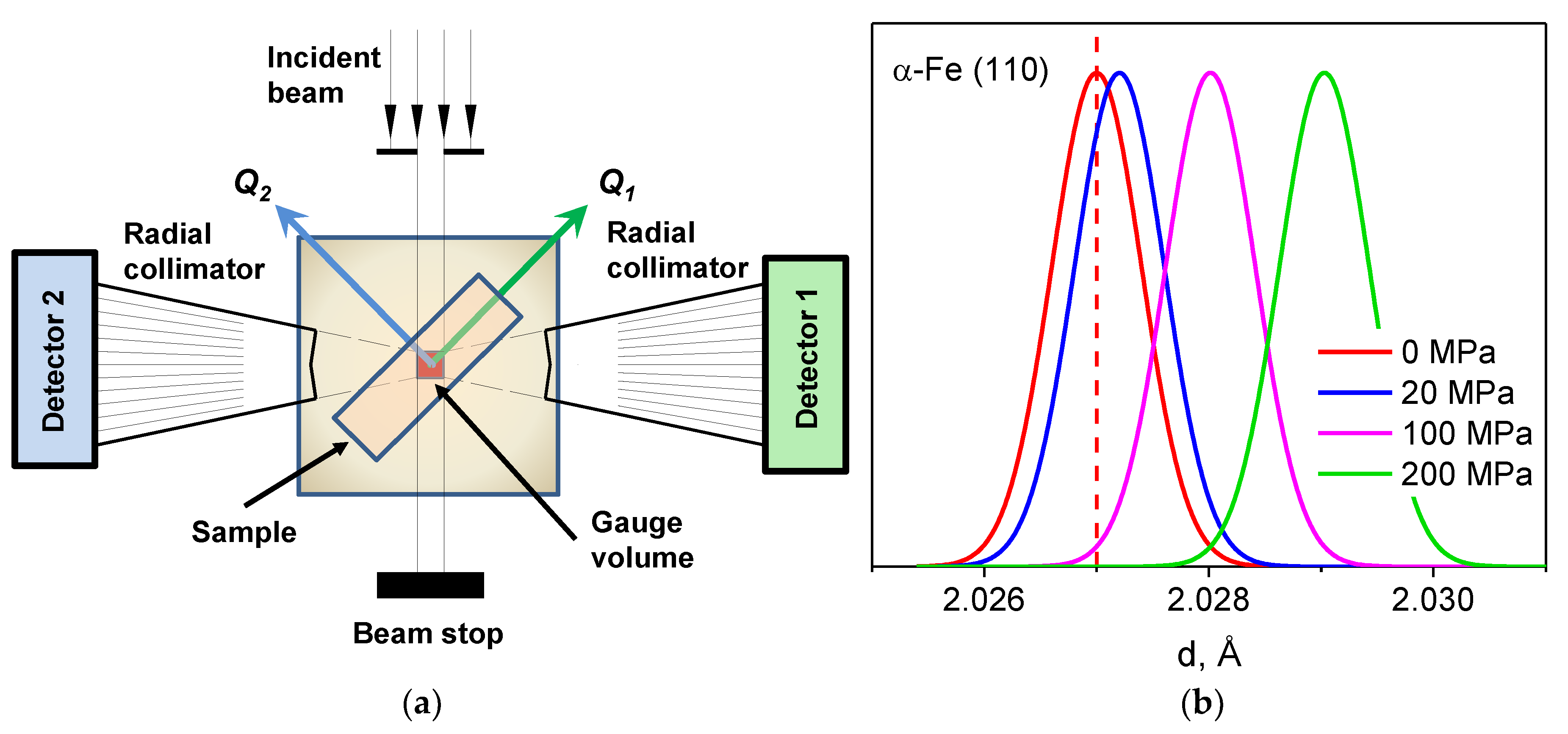
The essence of the diffraction method for studying stresses is rather simple and, in a conventional layout of the experiment, consists of incident and scattered neutron beam shaping using diaphragms and/or radial collimators and the definition of a small gauge volume in the bulk of the specimen (Figure 1) [18]. The incident beam is usually formed using diaphragms with typical sizes from 1–2 mm to several cm, depending on the purpose of the experiment. To define a gauge volume of an optimum shape in the studied specimen, at the scattered beam, radial collimators with many (about several tens) vertical slits formed by Mylar films with gadolinium oxide coating are often used. A radial collimator is placed at a quite large fixed distance (usually 150 ÷ 450 mm) from the specimen and provides a good spatial resolution of the level of 1–2 mm along the incident neutron beam direction. The lattice strain is measured in the direction parallel to the neutron scattering vector Q. The sample region under study is scanned using the gauge volume by moving the sample in the required directions. In this case, relative shifts of diffraction peaks from the positions defined by unit cell parameters of an unstrained material are measured.
Based on known values of the Young’s modulus, the required interplanar spacing measurement accuracy can be estimated, so that the σ determination error does not exceed, e.g., 20 MPa, which is, as a rule, quite sufficient for engineering calculations. For aluminum, E ≈ 70 GPa, hence, it is sufficient to measure Δa/a0 with an accuracy of 3 × 10⁻⁴; for steel, E ≈ 200 GPa, and the accuracy should be better than 1 × 10⁻⁴. These requirements appreciably exceed the capability of conventional neutron diffractometers with a typical resolution level of ~1–2%. Thus, for residual stresses studies, a diffractometer with an order of magnitude better resolution is needed. Existing practice has shown that a required accuracy can be achieved for diffractometers with monochromatic neutron beams, operating at stationary reactors, and for TOF diffractometers operating at pulsed neutron sources [19]. Without going into the details of experiments in these two cases, it should be noted that a main advantage of a constant wavelength instrument is a higher luminosity and, hence, the possibility of sample scanning with a good spatial resolution. In the case of a TOF instrument, a fixed and most optimal 90° experimental geometry is easily implemented and, in contrast to the former case, several diffraction peaks are simultaneously measured, which allows the analysis of strain anisotropy.
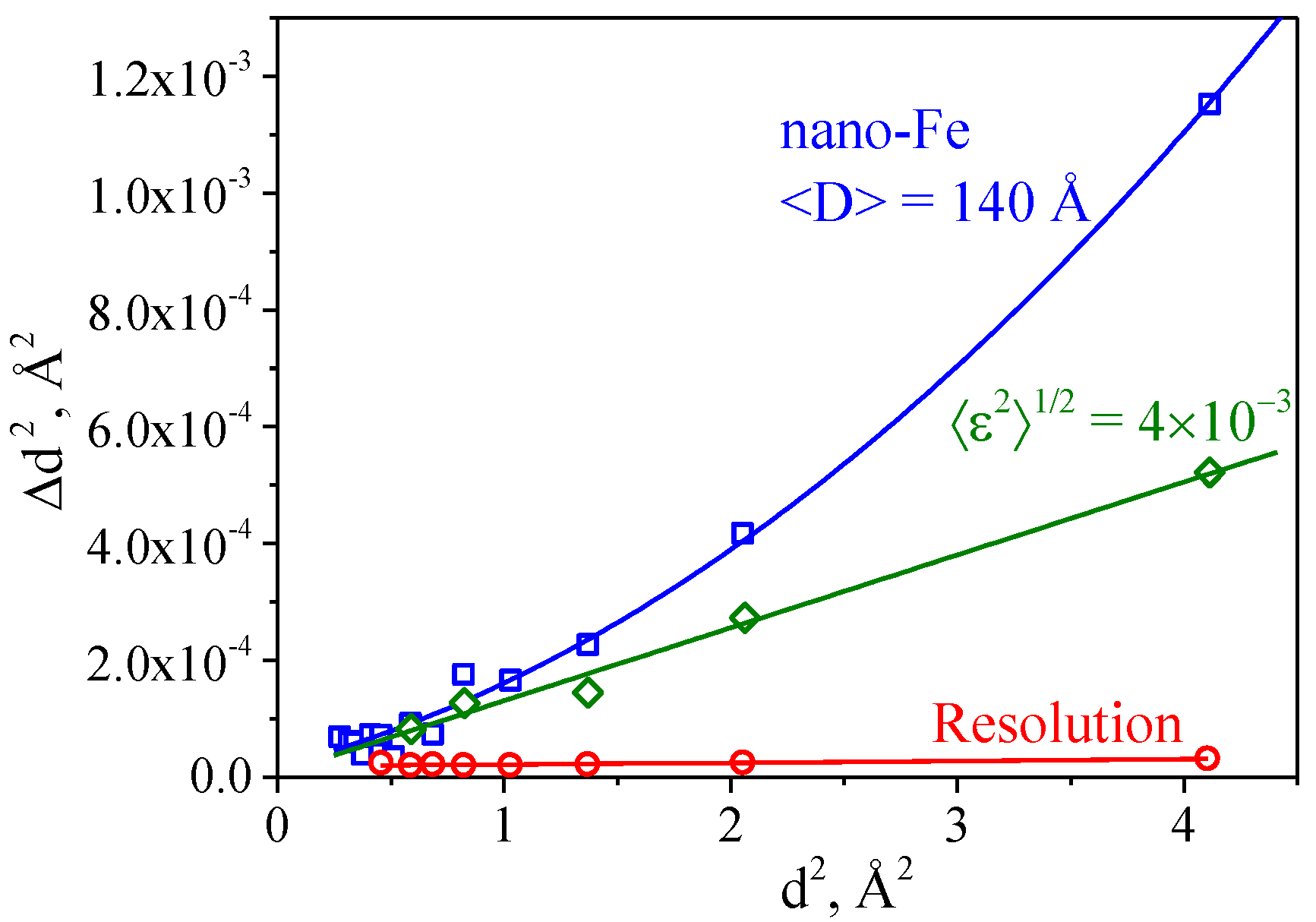
An important possibility for microstructure investigation is an analysis of the width and shape of a diffraction peak, which can provide data on crystal lattice microstrain and crystallite size [20]. TOF diffractometers at pulsed sources have a good potential for materials’ microstructure characterization due to the simplicity of the functional relationship between the instrument resolution R(d) and the interplanar spacing dhkl, which is almost independent of dhkl within a fairly wide range. In addition, TOF instruments exhibit a rather wide range of interplanar spacing and, consequently, possess a large number of simultaneously observed diffraction peaks with the almost similar contribution of the resolution function to their widths. This enables one to estimate lattice microstrain and the size of coherently scattering domains (crystallites) from diffraction peak widths in a rather simple way [21,22] (Figure 2):
where W is the peak width, C1 and C2 are the constants defining the diffractometer resolution function and known from measurements with a reference sample, C3 = 〈ε2〉 = (Δa/a)2 is the unit cell parameter dispersion (microstrain), and C4 ~ 1/〈D〉2 is the constant related to the crystallite size.
W2 = C1 + C2 d2 + C3 d2 + C4 d4,
The resolution of the neutron TOF diffractometer in a first approximation is defined by three terms,
where Δt0 is the neutron pulse width, t = CLsinθdhkl is the total time-of-flight (μs), and L is the neutron source–detector distance (m). The first term is the time-of-flight uncertainty, the second term includes all geometrical uncertainties associated with scattering at various angles, and the third term is the uncertainty in the flight path length. The resolution will improve as the Bragg angle approaches 90°, as the pulse width decreases, and as the flight distance increases. For neutron sources with a short pulse, the thermal neutron pulse width can be decreased to ~20 μs/Å; as the flight path length increases to 100 m, the resolution can be improved to 0.001 and, if required, to 0.0005.
R = Δd/d = [(Δt0/t)2 + (Δθ/tanθ)2 + (ΔL/L)2]1/2,
For neutron sources with long pulses, e.g., the IBR-2 pulsed reactor, such a way to achieve a high resolution is a priori unacceptable; the only practical way is to use the RTOF method in combination with a Fourier chopper [10], which provides a higher luminosity of experiments in comparison with other correlation techniques. In the RTOF method [23], the spectrum acquisition is performed with continuous variation of the rotation frequency of the Fourier chopper from zero to a certain maximal value Ωmax. The modulation frequency of the neutron beam ω is defined by the rotational speed of the Fourier chopper Ω and by the number of slits transparent for thermal neutrons NS in the rotor disk: ω = ΩNS. In this case, the time component of the resolution function is defined by the resolution function of the Fourier chopper RC, which depends on a particular frequency distribution g(ω) and can be written as
where ωmax = ΩmaxNS is the maximum frequency of neutron beam intensity modulation. With a reasonable choice of g(ω), the effective neutron pulse width is defined by the maximum modulation frequency: ∆t0 ≈ 1/ωmax. For standard FSD parameters NS = 1024, Ωmax = 6000 rpm, and ωmax = 102.4 kHz, the effective neutron pulse width is reduced to ∆t0 ≈ 10 μs. This means that even at a chopper–detector flight distance of ~6.6 m and scattering angle of 2θ = 90°, the contribution of the time component to the resolution function can be ∆t0/t ≈ 2 × 10⁻³ at d = 2 Å [24].
When using thin detectors, the term ΔL/L in Equation (7) becomes negligible, and the geometrical contribution can be optimized based on the desirable relation between resolution and intensity. A typical solution is the choice of focusing geometry in the arrangement of detector elements, with parameters providing a geometrical contribution equal to the time contribution to the complete resolution function. To increase the luminosity of the TOF diffractometer and decrease the background level, the primary neutron beam is formed using a curved mirror neutron guide. In this case, the neutron spectrum is cut off from the side of short wavelengths due to the neutron guide curvature radius chosen from the condition of the absence of line-of-sight of the neutron moderator. A calculation shows that, at a total flight path length from the source to the sample of ~20 m and a horizontal cross section of the neutron guide of ≤1 cm, the curvature radius can be sufficiently large to pass neutrons up to λ ≈ 1 Å. In this case, the number of simultaneously observed diffraction peaks, even for materials with small unit cell sizes (steel, aluminum), is about ten, which is sufficient to analyze strain/stress anisotropy. Furthermore, a sample place should be specially organized on the stress diffractometer, i.e., the possibility of installing large and heavy equipment (goniometers, loading machines, etc.).
3. FSD Diffractometer at the IBR-2 Pulsed Reactor
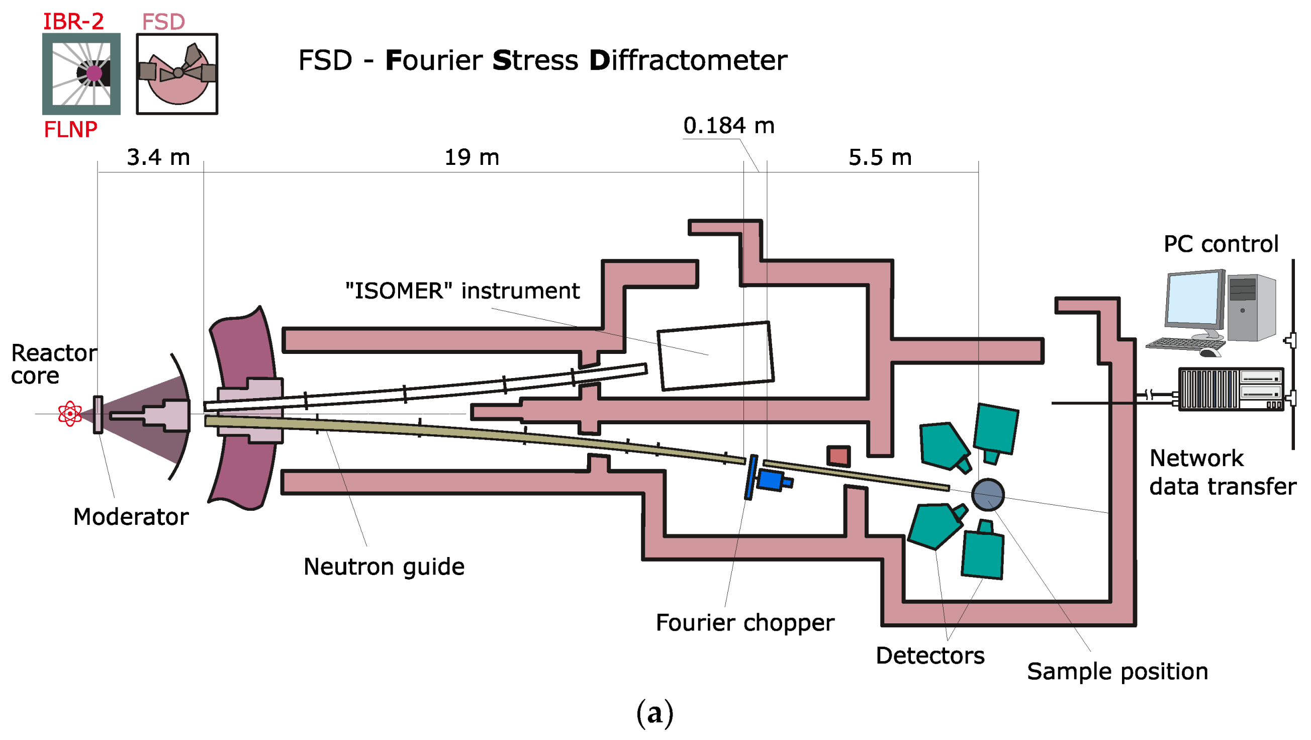
The basic functional units of the FSD diffractometer are the neutron source IBR-2 reactor with comb-like water moderator-generating thermal neutron pulses of ~340 μs with a frequency of 5 Hz; the curved mirror neutron guide eliminating fast neutrons and γ-rays from the neutron beam; the fast Fourier chopper providing neutron beam intensity modulation; the straight mirror neutron guide shaping the thermal neutron beam on the sample; the detector system consisting of detectors at scattering angles of ±90° and a backscattering detector; a heavy-load capacity goniometer, a diaphragm setting primary beam divergence, and radial collimators defining a gauge volume in the sample; and data acquisition electronics including an RTOF analyzer (Figure 3) [25]. The FSD diffractometer automation system [26] allows local or remote control of the experiment.
Mirror neutron guide. The neutron beam on the sample is formed by the mirror neutron guide made of high-quality borated (14% boron) K8 glass that is 19 mm thick with a Ni coating (m = 1). The neutron guide consists of two parts: one is 19 m long and bent with a curvature radius of R = 2864.8 m; the other is straight and 5.01 m long. The neutron guide is cone-shaped in the vertical plane with cross sections of 10 × 155 mm2 at the curved part input, 10 × 91.8 mm2 at the curved part output and at the straight part input, and 10 × 75 mm2 at the straight part output. At the Fourier chopper removed from the beam, the total thermal neutron flux at the sample position is 1.8 × 10⁶ neutron/cm2⋅sec; it decreases to 3.7 × 10⁵ neutron/cm2⋅sec due to a finite transmittance of the Fourier chopper.
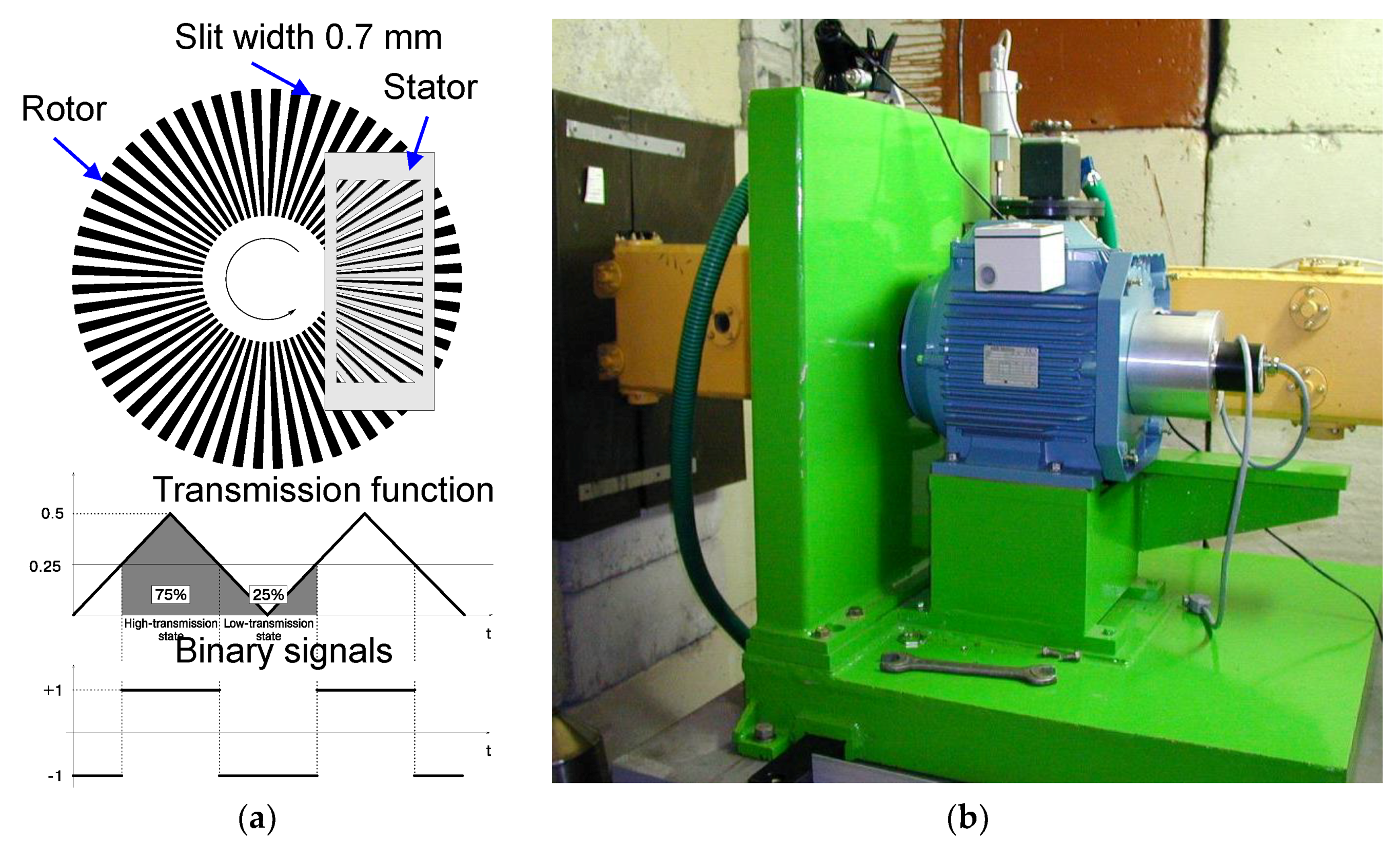
Fourier chopper. The Fourier chopper consists of a rotor disk that is 540 mm in diameter, installed on the motor axis, and a stator plate fixed on the stage (Figure 4a). The disk and plate are made of high-strength aluminum alloy. At the disk periphery, on the radius of 229 mm, there are 1024 radial slits 60 mm long and 0.7026 mm wide, filled with a Gd2O3 layer of a 0.8 mm thickness. Similar slits are made on the stator plate. The chopper is rotated by an M2AA 132SB-2 asynchronous bipolar motor (ABB Motors, Karlstad, Sweden) with a power of 7.5 kW. An incremental optical encoder TEKEL TK560 (Italsensor s.r.l., Pinerolo, Italy) with 1024 native pulses per revolution is fixed on the motor axis for measuring the disk velocity and for generating a pickup signal coming to the RTOF analyzer (Figure 4b). The motor is supplied by a VECTOR VBE750 control drive (Control Techniques, Telford, UK) with a built-in microcomputer, which receives information about the disk velocity and acceleration.
Detector system. In developing the detector system for the stress diffractometer, two mutually exclusive requirements should be satisfied: the solid angle of the detector system should be large enough to acquire statistics from a small sample volume for a reasonable exposition time; and the contribution of the detector system to the geometrical component of the resolution function should not exceed the time component to retain the high resolution of the instrument. There are two well-known versions of such a type of detector used on TOF diffractometers: position-sensitive systems and detectors with geometrical TOF focusing during diffraction [27]. However, the need to use the correlation principle of data recording in Fourier diffractometry almost excludes the possibility of using the position detector in this method. On the contrary, as for TOF focusing, it is successfully used on all operating Fourier diffractometers. A disadvantage of this method is a significant disproportion of the effective solid angle of the detector with its actual geometrical sizes. Progress in the development of relatively low-cost correlation electronics based on digital signal processors made it possible to propose a new principle of the development of the FSD detector system, namely, the multi-element detector with combined electronic and geometrical focusing [28]. The schematic representation of such a detector, called the ASTRA, is shown in Figure 5. Each detector element is a counter based on an ZnS(Ag) scintillation screen with a sensitive layer thickness of 0.42 mm and several hundred square centimeters in area. The scintillation screen consists of a powder mixture of 6LiF crystals (nuclear active additive) and ZnS(Ag) (scintillator) fixed in a Plexiglas optical matrix. The screen flexibility allows an approximation of the TOF focusing surface by conical surface segments with the required accuracy. Such an approximation method excludes dead areas on the sensitive layer and increases the quality of geometrical focusing. The detector efficiency is mostly defined by the 6Li concentration in the screen and is ~60%.
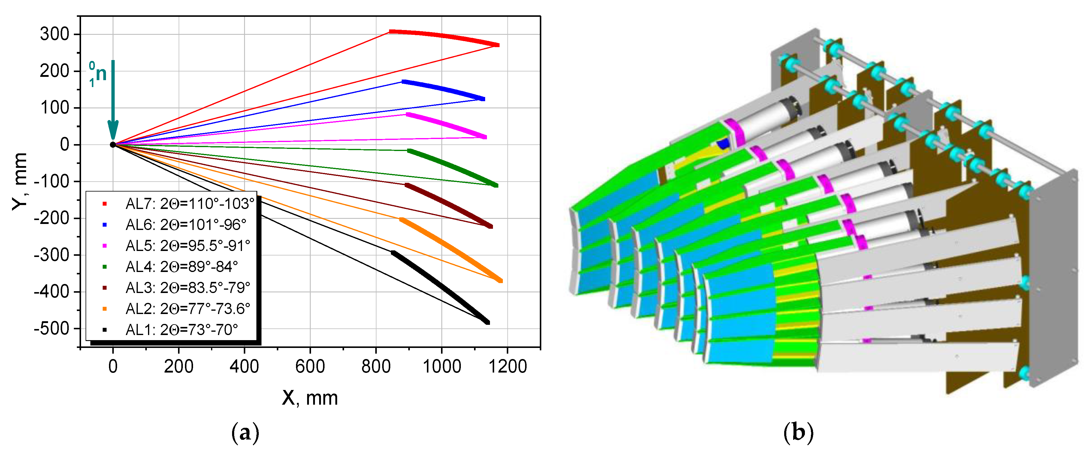
In the final version (Figure 6a), the FSD detector system consists of one backscattering detector (BS) at the scattering angle 2θ = 140° and two ASTRA detectors at the scattering angle 2θ = ± 90°. The BS detector is assembled from 16 6Li-based elements, which are spatially arranged according to the TOF focusing condition (Figure 6b). Each ASTRA detector includes seven independent TOF focused ZnS(Ag) elements, i.e., with independent outputs of electronic signals of elements [29]. The combined use of electronic and TOF focusing of the scattered neutron beam allows researchers to increase the solid angle up to ~0.16 sr for each ASTRA detector. This sharply increases the instrument luminosity while retaining the high resolution level in the interplanar spacing dhkl. Currently, eight elements (among 14 planned) of ASTRA 90°-detectors are installed on the FSD. The application of the RTOF method makes it possible to obtain high-resolution (Δd/d ≈ 0.2 ÷ 0.4%) diffraction spectra with the fairly short flight distance (~6.6 m) between the Fourier chopper and neutron detectors [30].
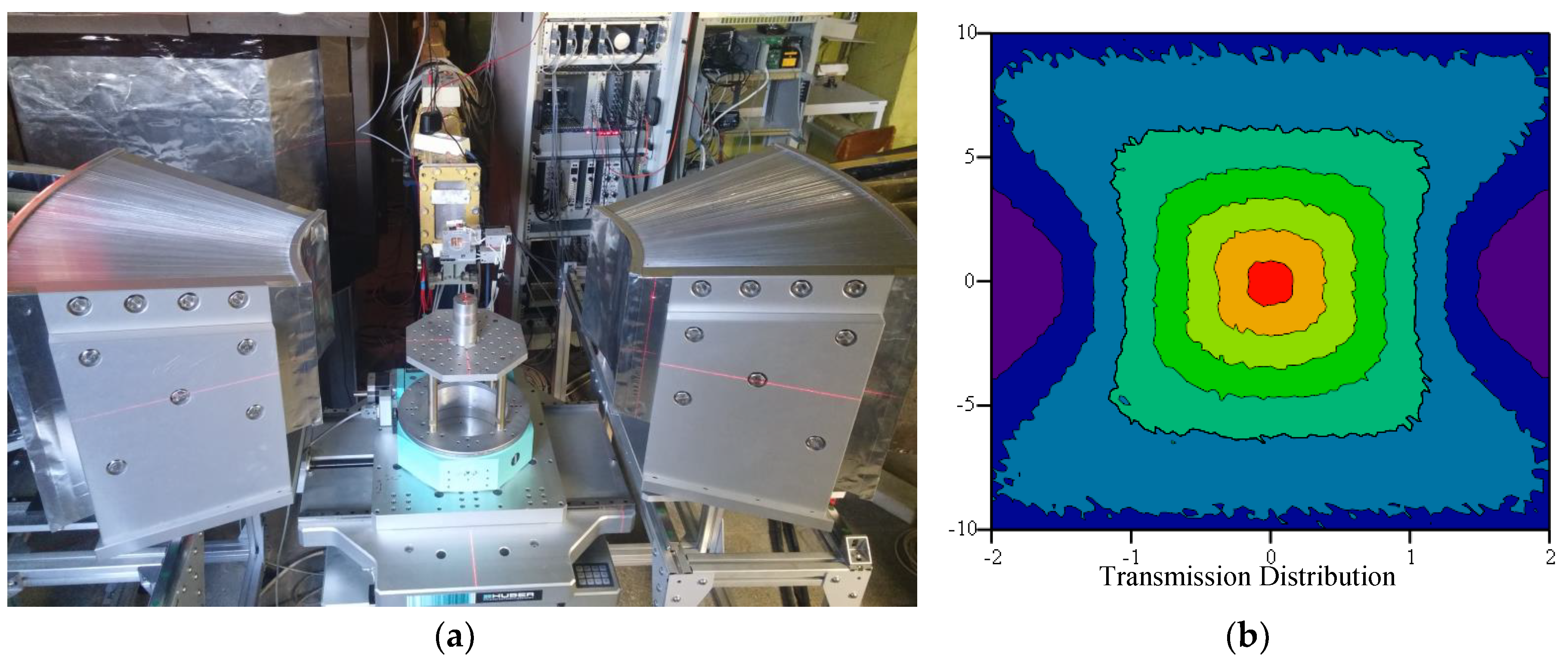
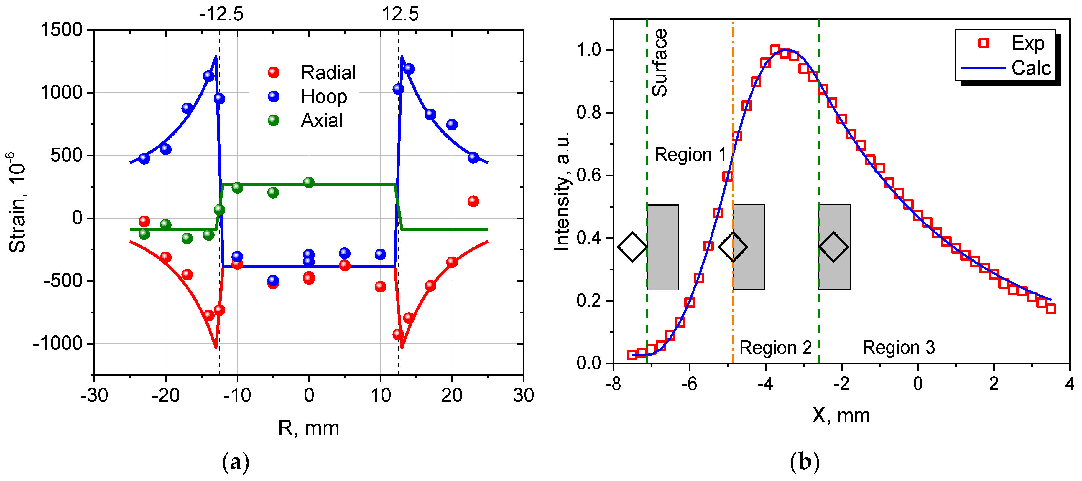
Gauge volume definition with radial collimator. To form the incident neutron beam, a diaphragm with precision step motors and variable aperture (0–30 mm for width and 0–80 mm for height) is installed on the neutron guide exit of FSD. The experimentally estimated horizontal and vertical divergences of the incident beam are 0.001 and 0.002 radians, correspondingly. The scattered neutron beams are formed using two new multi-slit radial collimators with a wide acceptance angle of ±20° (Figure 7). This allows a definition of the gauge volume in the studied sample. The performed experiments showed that the radial collimators provide a spatial resolution of ~1.8 mm with an improved neutron transmission capacity and precisely form the required gauge volume within the studied sample. Performed test measurements with the VAMAS [31] shrink-fit ring and plug standard round robin sample with known residual stress profiles confirmed the high sensitivity of the FSD instrument to strain gradients and the high accuracy of the measured strain values (Figure 8a).
Using neutron scanning, the gauge volume position can be easily determined with respect to the sample surface; then, its position in the sample bulk can also be accurately positioned in further strain measurements. The neutron scanning method involves measuring the dependence of the diffraction peak intensity on the gauge volume center position. The sample is sequentially displaced so that the gauge volume is gradually immersed into the sample (Figure 8b). The initial point in the plot corresponds to the gauge volume position outside the sample; in this case, the diffraction peak intensity is zero (there is no diffraction from the sample material). Then, the gauge volume gradually enters the sample, hence, the diffraction peak intensity, which is proportional to the scattering material volume, begins to increase. The point of the maximum in the plot approximately corresponds to the position at which the gauge volume is completely immersed into the sample. During further motion to the sample depth, the scattering material volume remains unchanged; however, the intensity begins to decrease slowly due to neutron absorption according to the exponential law
where μ is the material attenuation coefficient and D is the total neutron path in the sample. Thus, neutron scanning allows the determination of the gauge volume in the sample with a high enough accuracy (~0.1 mm).
List-mode DAQ system. Recently, a new unified MPD (Multi Point Detector) DAQ unit intended for data registration from individual neutron detector elements was elaborated in FLNP JINR [32]. The electronic part of the MPD unit is based on five ALTERA FPGAs and it is implemented on a modular principle. The elaborated MPD unit allows the connection of up to 240 detector elements. On the FSD diffractometer, the MPD-32 DAQ unit with 32 input detector signals is installed for routine operation. Due to the peculiarities of the RTOF method, four main types of events are registered by MPD-32 on FSD: detector events, reactor pulses, and rising and falling fronts of Fourier chopper pickup signals. The MPD-32 unit can operate simultaneously in two modes: histogram-mode of TOF-spectra accumulation and list-mode of raw data transfer [33]. In histogram-mode, the TOF spectrum (low-resolution spectrum) is accumulated in internal memory (64 Mb) of the MPD unit with a programmable fixed number of channels and channel widths, and can be visualized on screen online. In list-mode, raw data events are recorded as a list of 32-bit words with a total maximum data flow rate of 8 × 10⁶ events/sec. and maximum sampling frequency of 62.5 MHz, which corresponds to a discretization time of 16 ns. Thus, in this case, the absolute time of each event (timestamp) is defined with a high precision and is written as raw data on a computer HDD. The elaborated LM-algorithm provides a fast a posteriori reconstruction of high-resolution neutron diffraction spectra (RTOF spectra) from raw data in a wide dhkl range with flexibly configurable parameters of the TOF-scale., i.e., number of channels in the spectrum, channel width, spectrum and strobe pulse delays, flight paths relation coefficient, etc. If necessary, this procedure can be performed repeatedly without additional measurements. Moreover, the LM algorithm includes some auxiliary opportunities for spectra correction (chopper phase shift correction, detector signal filtering, precise electronic focusing of individual detector elements into the single TOF scale, real frequency window reconstruction, etc.).
The main idea of the RTOF method is to examine the registration probability (high or low) for detected neutrons [5]. This is realized by the reverse analysis of “open” and “closed” states of the neutron source and Fourier chopper for each detector event. Registering neutrons with continuous beam modulation according to the particular law (frequency window g(ω)), it is possible to obtain the TOF distribution of elastically scattered neutrons. In simplified form, the unity is added to the analyzer memory cell if both the neutron source and the chopper are in the “open” state.
The neutron intensity measured by RTOF method at a pulsed neutron source can be described as [10]:
where RС is the resolution function of the Fourier chopper (see Equation (8)), RS is the function describing the neutron pulse from the source, σ is the coherent scattering cross section of the sample, B is the conventional background, and c ≈ 1 is a constant.
The width of the RS function is about WS ≈ 340 μs for the IBR-2 reactor, while the width of RС is defined by the maximal modulation frequency ωmax of the Fourier chopper and it is about ∆t0 ≈ 10 μs for the FSD diffractometer. Thus, the first term in Equation (10) is a narrow peak with a width of 10 μs, and the second one is the broad peak-like distribution with a width of 340 μs, which is called the correlation background.
The + or − sign before the first term in Equation (10) corresponds to correlation patterns I+(t) (“positive”) and I−(t) (“negative”) accumulated with non-inverted and inverted pickup signals of the Fourier chopper, correspondingly (Figure 9). The non-inverted binary pickup signal is 1 for the high transmission (“open”) state of the Fourier chopper and 0 for the low-transmission (“closed”) state, whereas the inverted pickup signal is 1 for the low-transmission state and 0 for the high-transmission state. The high-resolution diffraction RTOF spectrum is calculated as a difference of “positive” and “negative” patterns: H(t) = I+(t) – I–(t). The high-resolution spectrum H(t) contains narrow diffraction Bragg peaks with widths corresponding to the diffractometer resolution function for a certain interplanar spacing dhkl. The high-resolution peak position in the TOF-scale is defined as (cf. Equation (1)):
where LRTOF is the flight path between the Fourier chopper and detector.
Electronic focusing of detector elements. Usually, during stress scanning experiments, the radial collimators are used in front of the 90°-detectors for small gauge volume selection in the depth of the sample. Therefore, the intensity factor is a very important parameter and the whole detector solid angle should be used in such experiments. For the summation of the spectra from the individual elements of ASTRA ±90°-detectors, the electronic focusing method is used. This method implies the use of scale coefficients for each detector element and measuring RTOF spectra with individual channel widths τi,
where Li, L0 are the flight paths (i.e. distance between the Fourier chopper and neutron detector); θi, θ0 are the scattering angles; and τi, τ0 are the RTOF channel widths for the i-th and basic detectors, respectively.
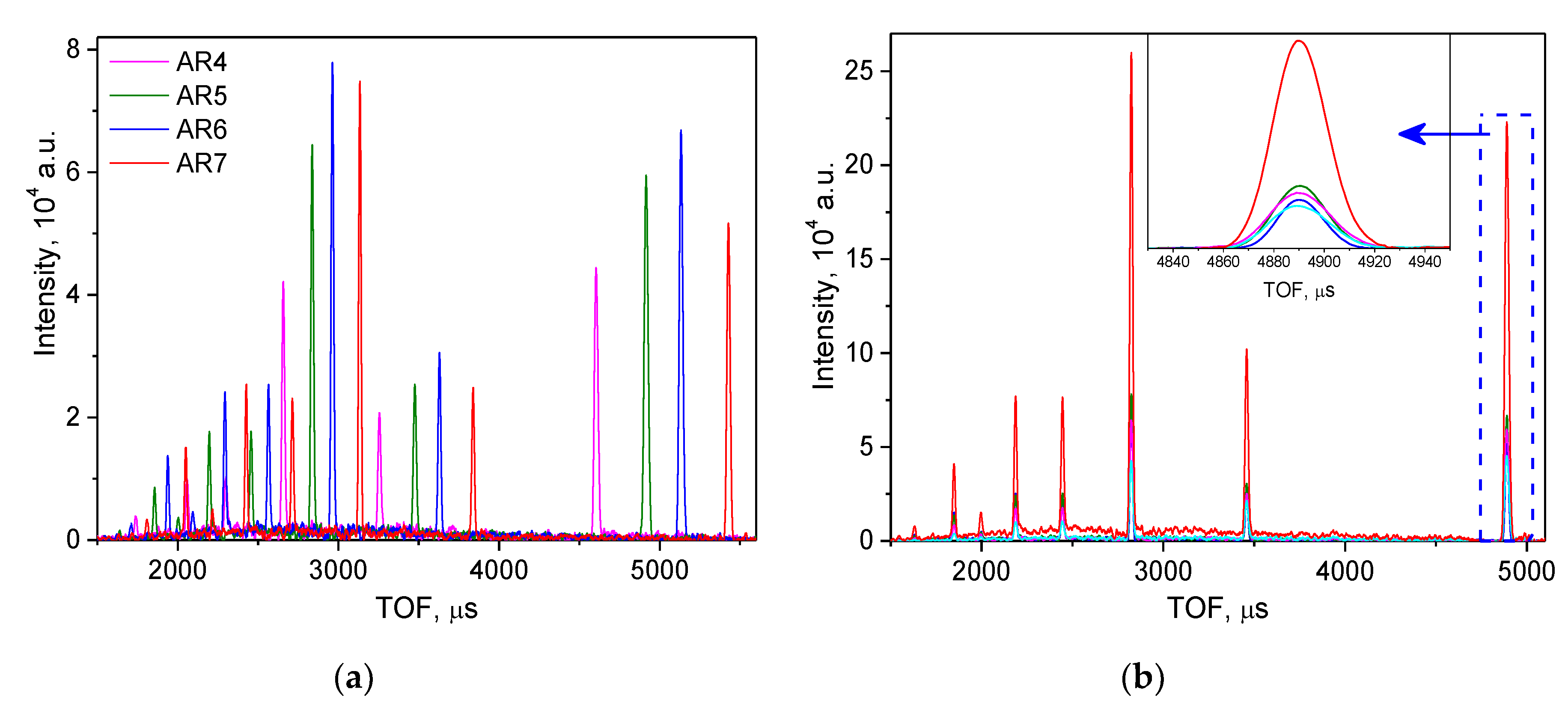
Usually, τi are real (noninteger) numbers and RTOF spectra with such channel width values are readily reconstructed from raw list-mode data with the required accuracy. Therefore, all spectra are reduced to a unified TOF scale corresponding to the basic detector with parameters L0, θ0, and τ0, and can be summed channel by channel. The final diffraction spectrum is characterized by a multiple increase in the intensity at the same resolution level as for the spectra from individual detector elements (Figure 10). Thus, the luminosity of the experiment on FSD is increased by a factor of four using electronic focusing for all elements of ASTRA ±90°-detectors. A similar approach was used for additional fine tuning of individual elements of the BS detector with geometrical TOF focusing, which allowed the detector resolution to improve by ~5%.
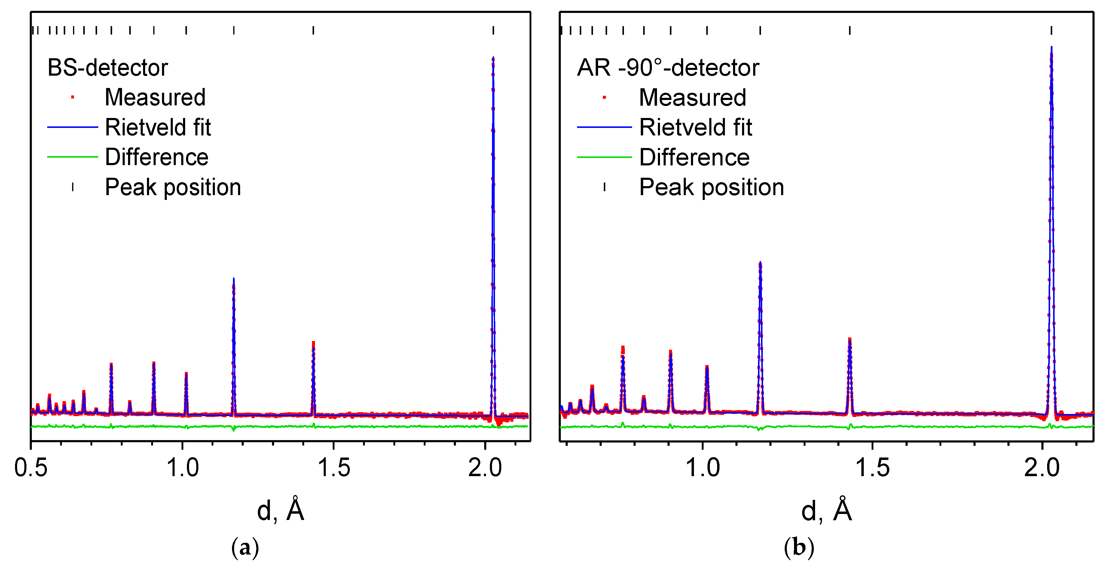
FSD diffractometer performance. To study the main characteristics of the FSD diffractometer, a number of test experiments were performed to estimate the instrument resolution, sensitivity to the spatial distribution of strains, and the possibility of studying typical structural materials under external loads. The spectral distribution of the incident neutron beam intensity on the FSD allows efficient operation at λ ≥ 1 Å. This makes it possible to measure diffraction spectra in the ranges dhkl = 0.63 ÷ 6.7 Å at 2θ = 90° and dhkl = 0.51 ÷ 5.4 Å at 2θ = 140°, which is an optimum range for most structural materials used in industry. The typical high-resolution diffraction spectra measured on the α-Fe reference powder sample at a maximum rotation speed of the Fourier chopper Ωmax = 6000 rpm are shown in (Figure 11).
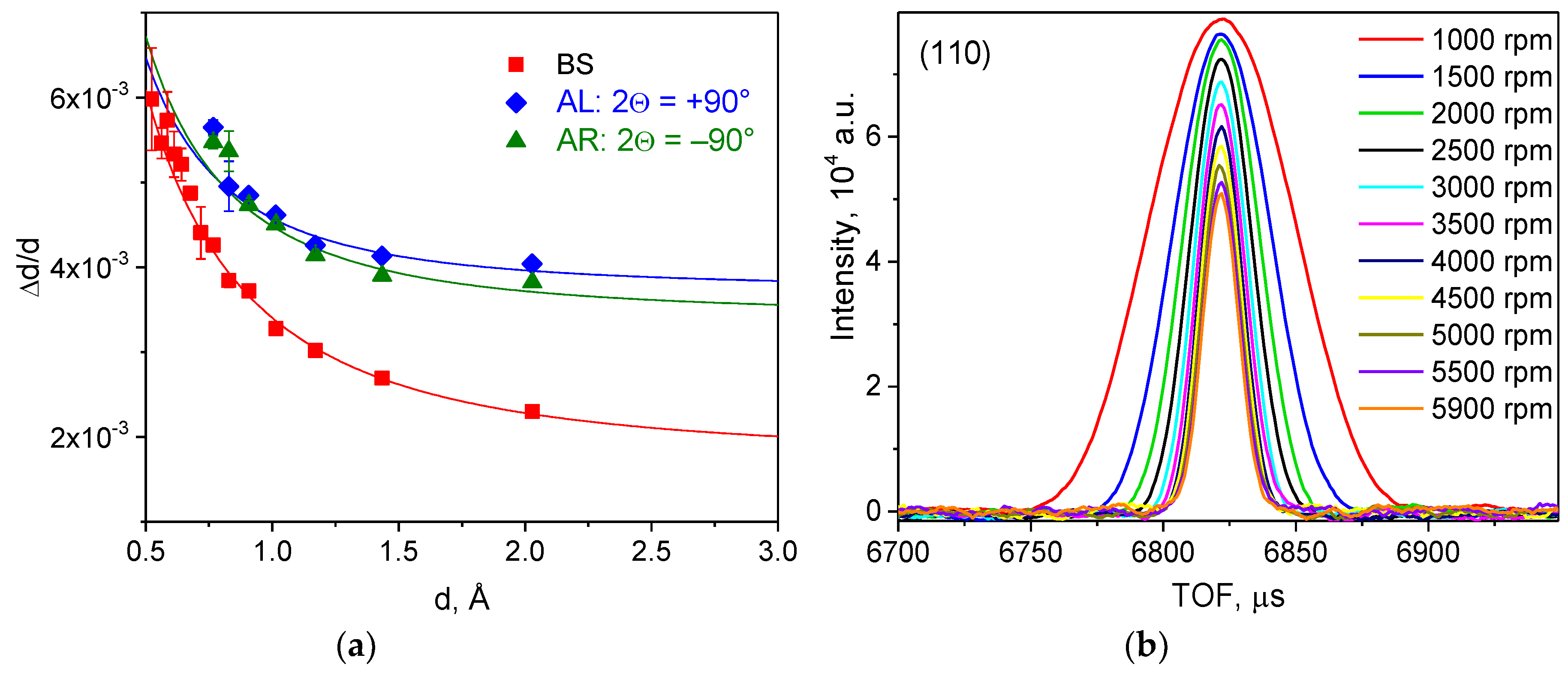
An analysis of the diffractometer resolution function showed that FSD detectors indeed have a necessary resolution level in the interplanar spacing: Δd/d ≈ 2.3 ×⋅10–3 for the backscattering detector BS and Δd/d ≈ 4 × 10⁻³ for both ASTRA ±90°-detectors at d = 2 Å and at a maximum rotation speed of the Fourier chopper Ωmax = 6000 rpm (Figure 12a). Furthermore, the dependence of the shape of an individual diffraction peak on the maximum speed of the Fourier chopper and resolution function for all detectors were investigated (Figure 12b). According to expectations, the effective neutron pulse width decreases as 1/ωmax, reaching a minimum of ~10 μs. Thus, the diffractometer parameters can be optimized, taking into account the required accuracy of peak position determination and scheduled beamtime. Main parameters of the FSD diffractometer are given in Table 1.
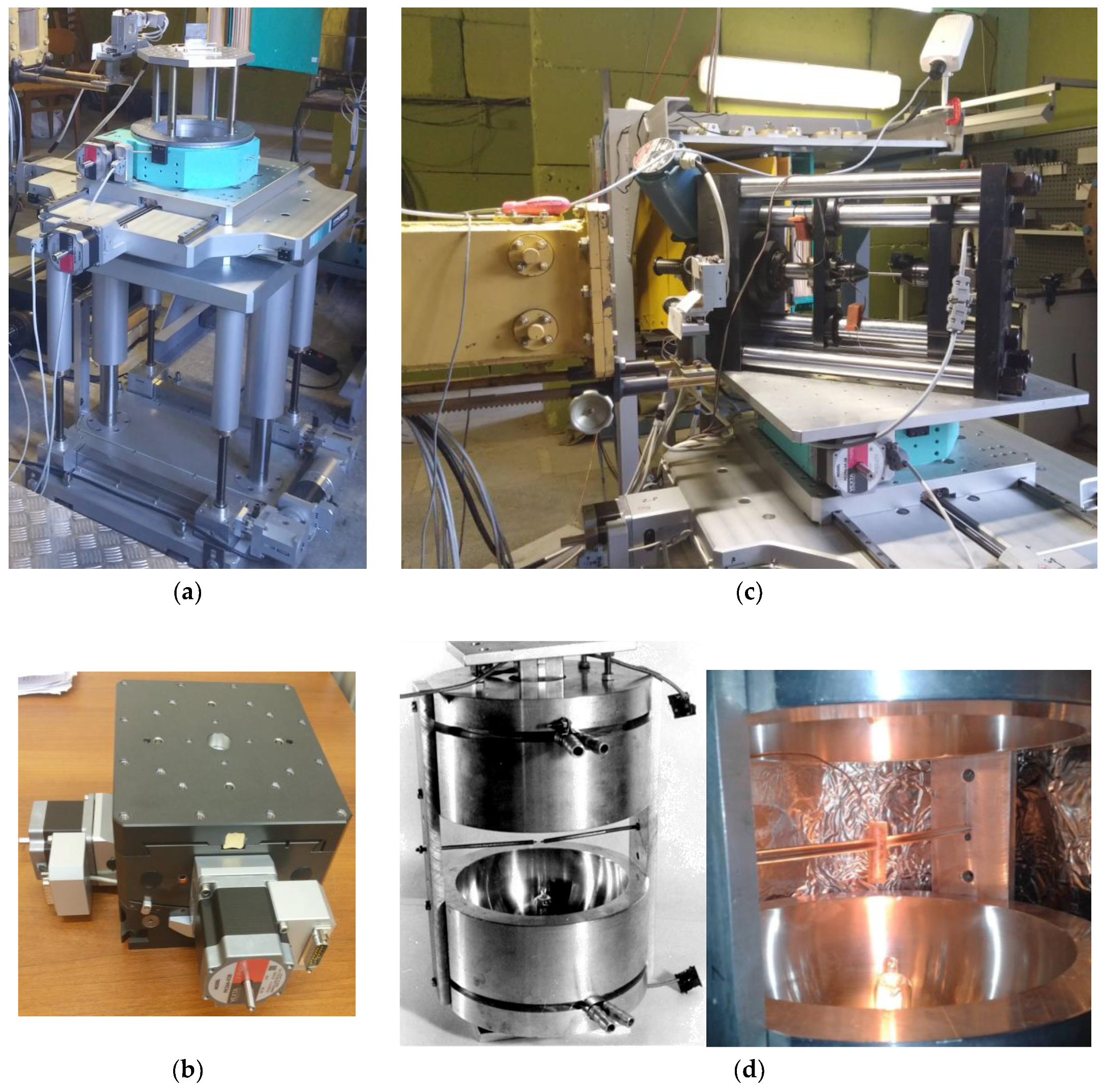
Sample environment. Available supplementary equipment integrated into the experiment control system makes it possible to provide various conditions (load, temperature, etc.) at the sample. For precise sample positioning, a four-axis (X, Y, Z, Ω) HUBER goniometer with the maximal carrying capacity of 300 kg is used (Figure 13a). It can be equipped with an additional goniometer head with ±15°-tilt (Figure 13b). To study the behavior of structural materials under an external load in situ in a neutron beam, an LM-29 uniaxial mechanical-type loading machine is used; it provides any required combination of external load and temperature, which considerably extends the range of possible experiments on the diffractometer. The device provides a tensile/compressive load at the sample of up to 29 kN. There is also the possibility to heat metallic samples by an electric current up to 800 °С (with temperature control). The main advantage of this loading machine is the almost slack-free load transfer to the sample (Figure 13c). For neutron diffraction experiments at elevated temperatures (up to 1000 °С) with small samples of typical dimensions of ~1 cm, the MF2000 water-cooled mirror furnace is used (Figure 13d). The furnace consists of two polished aluminum reflectors and two halogen lamps with temperature stabilization by the Lakeshore controller.
4. Experimental Results
A significant place in applied researches on the FSD diffractometer belongs to experiments for residual stress investigations in structural materials and industrial products after various technological operations. Another research area is the in situ study of the behavior of structural materials (composites, steels, alloys, ceramics, etc.) under various conditions (external load, temperature). Below, several examples of typical experiments performed on FSD are given.
4.1. Welding Residual Stresses
The neutron diffraction data are often used for a comparison with the results of calculations by the finite element method (FEM), for the consequent development of theoretical models for an adequate description of various technological processes and the correct estimation of the stress level over an entire product. For example, in [34], the residual stress distribution in a multi-pass butt-welded joint of the low alloyed steel S355J2+N was investigated. For the welding experiments, the Gas Metal Arc Welding (GMAW) method was used for the first welding pass and the Submerged Arc Welding (SAW) method was used for the second and third welding passes. The dimensions of the welded specimen were the following: 500 mm length, 300 mm width, and 20 mm thickness. The initial sample temperature as well the interpass temperature were always equal to room temperature.
For neutron diffraction experiments on FSD, a special specimen was cut from the entire multi-pass welded joint (Figure 14a). The neutron measurements were performed at the middle of the sample’s thickness, with a gauge volume of the size of 5 × 2 × 20 mm3 for Y- and Z-components and of the size of 5 × 2 × 5 mm3 for the X-component. The measured diffraction spectra were processed using full profile analysis based on the Rietveld method [35]. The average residual strain was determined as ε = (a − a0)/a0, where a is the lattice parameter for the studied specimen with residual stresses and a0 is the lattice parameter for stress-free reference material. The residual stress components were determined from the obtained strain values according to Equation (5). In the investigated specimen, the distribution of the residual stress tensor components over scan coordinate X alternate in sign and vary within wide limits (Figure 14b). The maximum of the residual stress distribution agrees rather well with the position of the weld seam. As would be expected, the residual stresses decrease sharply with distance from the weld seam region.
In addition to the neutron diffraction experiments, numerical calculations were performed by FEM. The developed model of the multi-pass welding process makes it possible to calculate the residual stress distributions depending on the welding process parameters for the most widespread structural materials. A comparison of the neutron data and the results of calculations carried out by the finite element method showed their good agreement, which demonstrates that the developed theoretical model of the welding process is reliable. This information can be used as a base for the development of specific technological recommendations to obtain the desired level and profile of residual stresses.
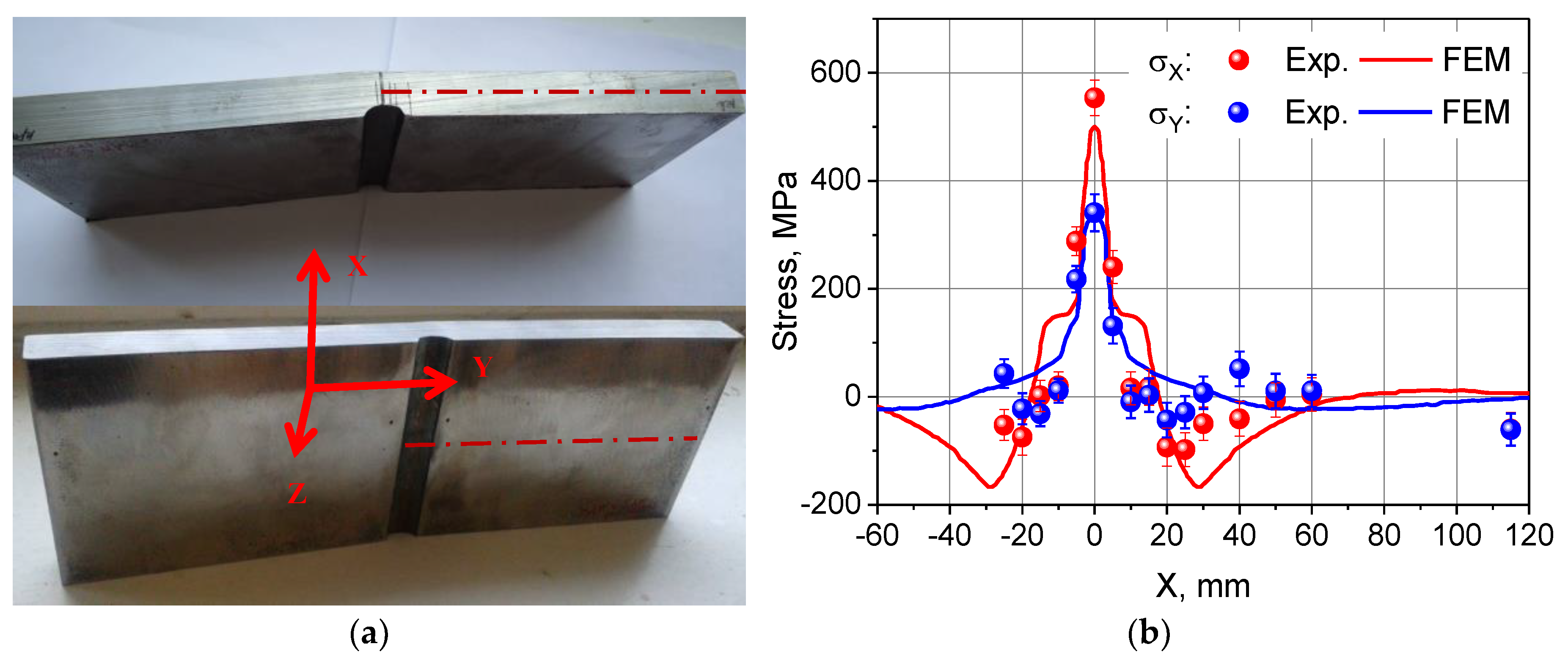
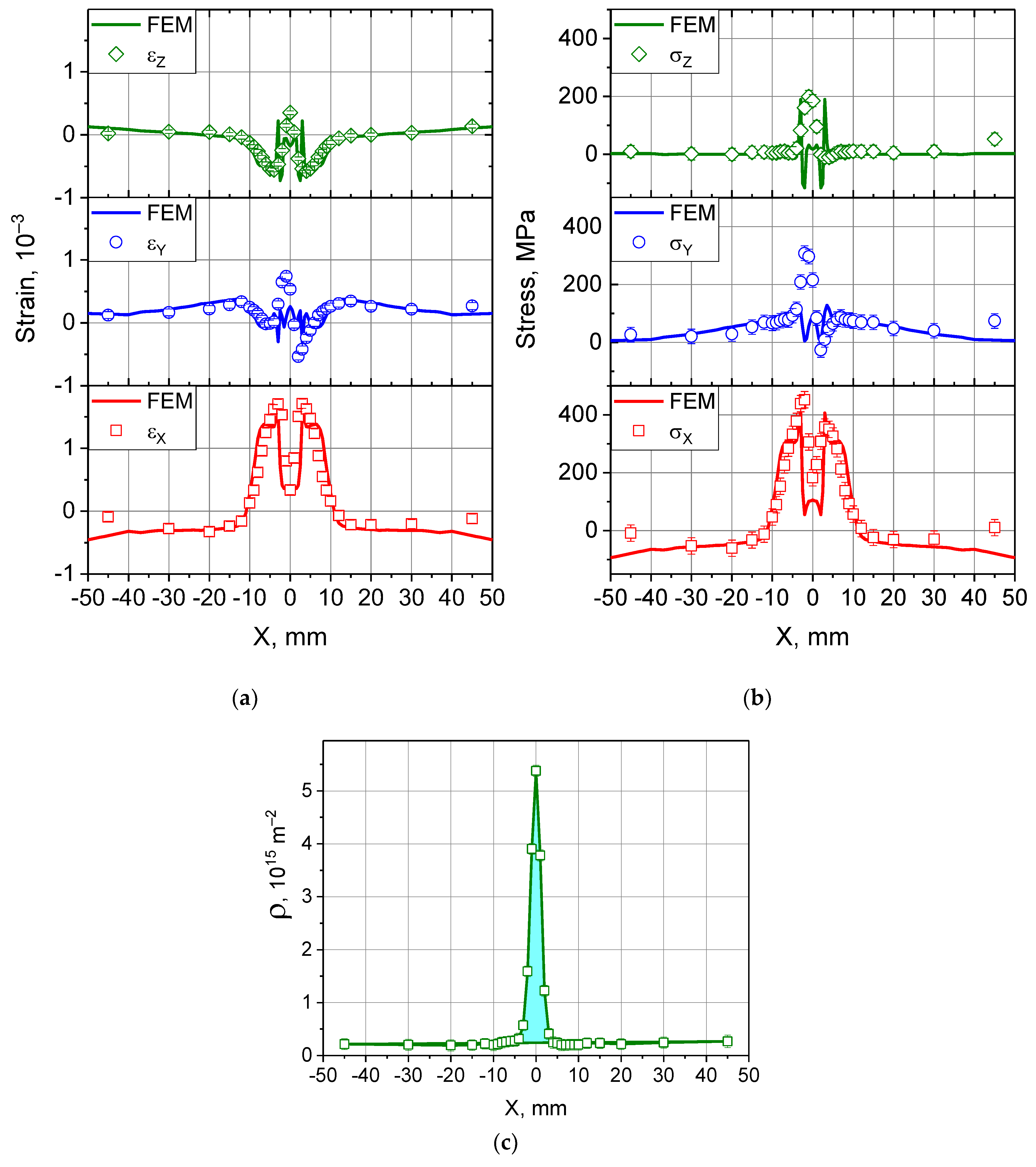
In similar research work [36], the residual stresses and microstrains in a thin C45 low-alloyed steel plate welded by a laser beam were investigated. The sample with dimensions of 100 × 100 × 2.5 mm3 was mounted on three points and welded by a solid-state laser beam using a six-axis robotic arm. The residual stress distribution in this laser beam welded (LBW) joint was investigated on an FSD diffractometer with a 2 × 2 × 10 mm3 gauge volume. The strain scanning was performed across the welding direction along a path on the middle of the length (Y = 50 mm) and in the middle plane (Z = 1.25 mm) of the specimen. The neutron diffraction results show a good agreement with FEM calculations for longitudinal and normal stress components (Figure 15).
The longitudinal residual stress exhibits two characteristic peaks at distances ±3 mm from the weld center, which corresponds to the boundaries of the heat-affected zones (HAZ). In the HAZ area (0 mm < X < 3 mm), a significant decrease of the longitudinal stress due to the martensite microstructure formation is observed. For the transverse residual stress component, the results can also be considered quite satisfactory. Nevertheless, the experimental data demonstrate a small but noticeable asymmetry, which can be explained by rapid non-equilibrium cooling after welding under conditions of rigid fixation of the sample.
In the welded joint and HAZ regions, significant diffraction peak broadening is often observed due to the change in the material microstructure. Usually, these effects are caused by crystallite size changes due to martensitic transformations and by the increase in the residual lattice microstrain, which directly characterizes the dislocation density in a material. From the broadening of diffraction peak widths, the level of residual microstrain was evaluated for the studied sample. It was found that the microstrain distribution exhibits a sharp gradient at the weld seam position (X = 0 mm) with a maximal level of ~4.8 × 10⁻³, which falls down to ~1 × 10⁻³ for regions outside the HAZ area. The estimated dislocation density varies from ~2 × 10¹⁴ m−2 for the base material to the maximal value of ~5.4 × 10¹⁵ m−2 at the weld seam center (Figure 15c).
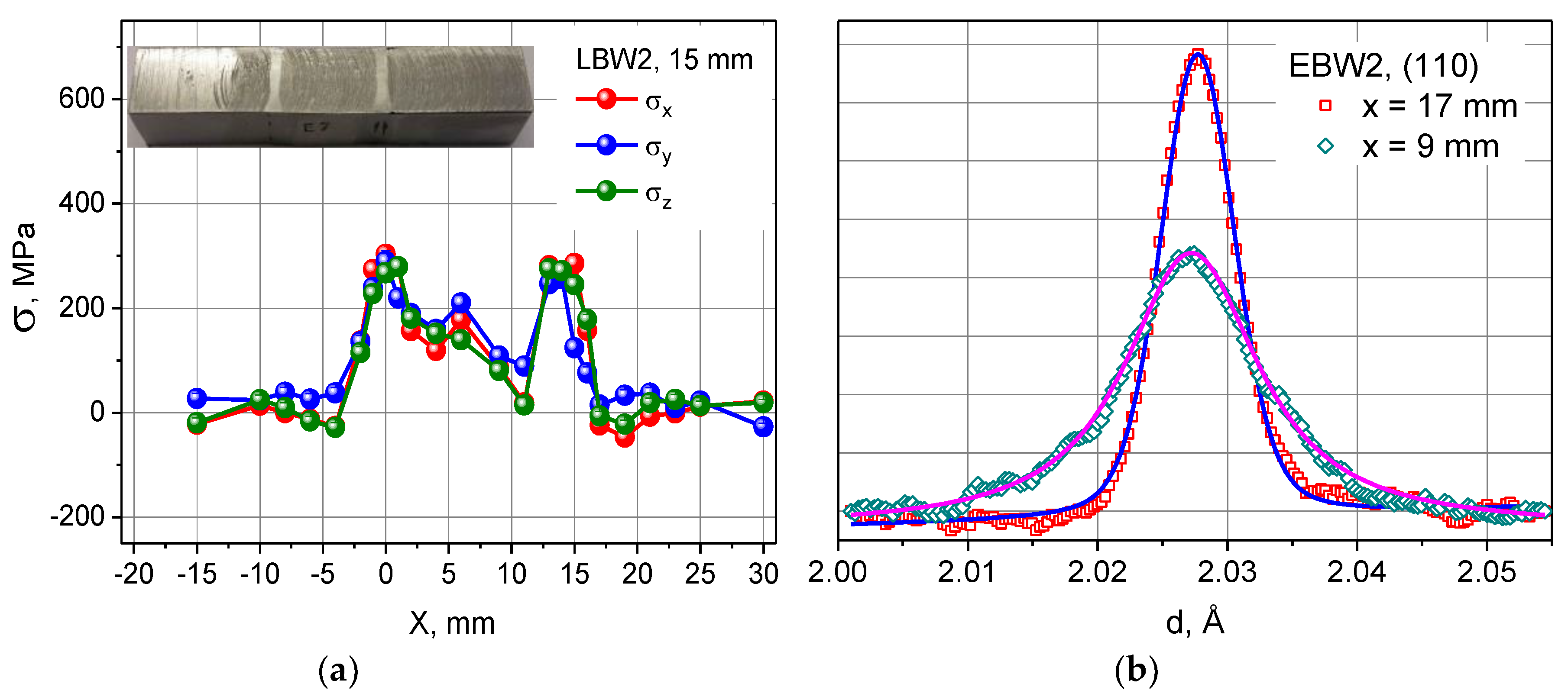
Changes in the reactor pressure vessel (RPV) material properties due to neutron irradiation are monitored by means of surveillance specimen programs, which are used for the realistic evaluation of RPV lifetime. Due to the limited number of surveillance specimens, their proper reconstitution procedure after Charpy impact tests is of great importance. In order to evaluate the feasibility of various reconstitution methods, the residual stress distribution and microstrain level in test Charpy specimens welded by the most common techniques (electron beam welding—EBW, laser beam welding—LBW, arc stud welding—ASW) were analyzed on FSD [37,38]. Welding techniques are based on the use of highly localized energy sources to fuse or soften the material at the weld joint. Due to the concentrated heat input and temperature gradients, significant residual stresses and distortions occur after the welding process [39] The level of residual stress depends to a large extent on the parameters of the welding procedure. The measured residual stress distribution exhibited alternating sign characters for all studied Charpy specimens (Figure 16a). Both EBW specimens demonstrated the lowest level of the residual stress varying from −85 MPa to 172 MPa for EBW1 and from −91 MPa to 308 MPa for EBW2, correspondingly. Two other specimens exhibited significantly higher stress levels: from −175 MPa to 570 MPa for LBW and from −204 MPa to 678 MPa for the ASW sample.
The pronounced peak broadening effect was observed at the centers of the welded joints due to the change in the material microstructure during the welding process (Figure 16b). For further analysis, the individual diffraction peaks were fitted by the Voigt function using the least-squares method. It is noteworthy that in the regions remote from the weld seam zone, the main contribution to the total peak width gives the Gaussian component of the peak. On the contrary, in the weld centers and HAZ regions, the predominant contribution is defined by the Lorentzian component, which points to a significant influence of the small sizes of crystallites on the peak broadening effect.
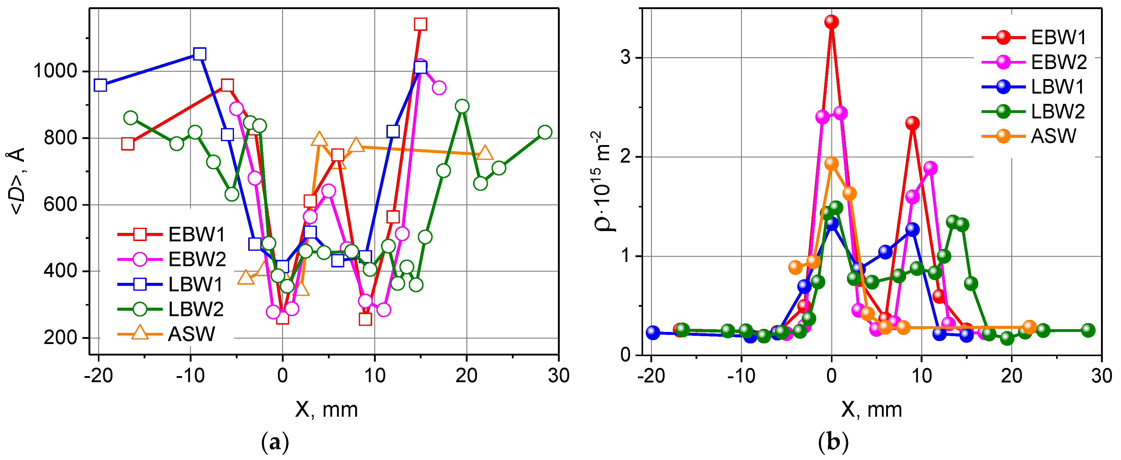
The volume-weighted crystallite size was estimated from (110) and (220) line profiles analysis according to the Warren-Averbach method [40] (Figure 17a). The effect of a small crystallite size, causing Lorentzian-type peak broadening, is clearly seen at the weld seam centers at X = 0 and X = 9 mm (X = 14 mm for LBW2 specimen). Using modified Williamson-Hall type dependencies Δd2(d2) [41,42], the anisotropic peak broadening was analyzed and the microstrain level and dislocation density were estimated for all studied samples. Similarly to microstrain, the distribution of the dislocation density exhibits quite high values at weld seams centers, reaching a maximal level of 2.9 × 10¹⁵ m−2 for EBW1, 2.1 × 10¹⁵ m−2 for EBW2, 1.2 × 10¹⁵ m−2 for LBW, and 1.7 × 10¹⁵ m−2 for ASW specimens, correspondingly. In regions away from weld seams it decreases sharply down to ~2 × 10¹⁴ m−2 (Figure 17b).
4.2. Mechanical Properties of Structural Materials
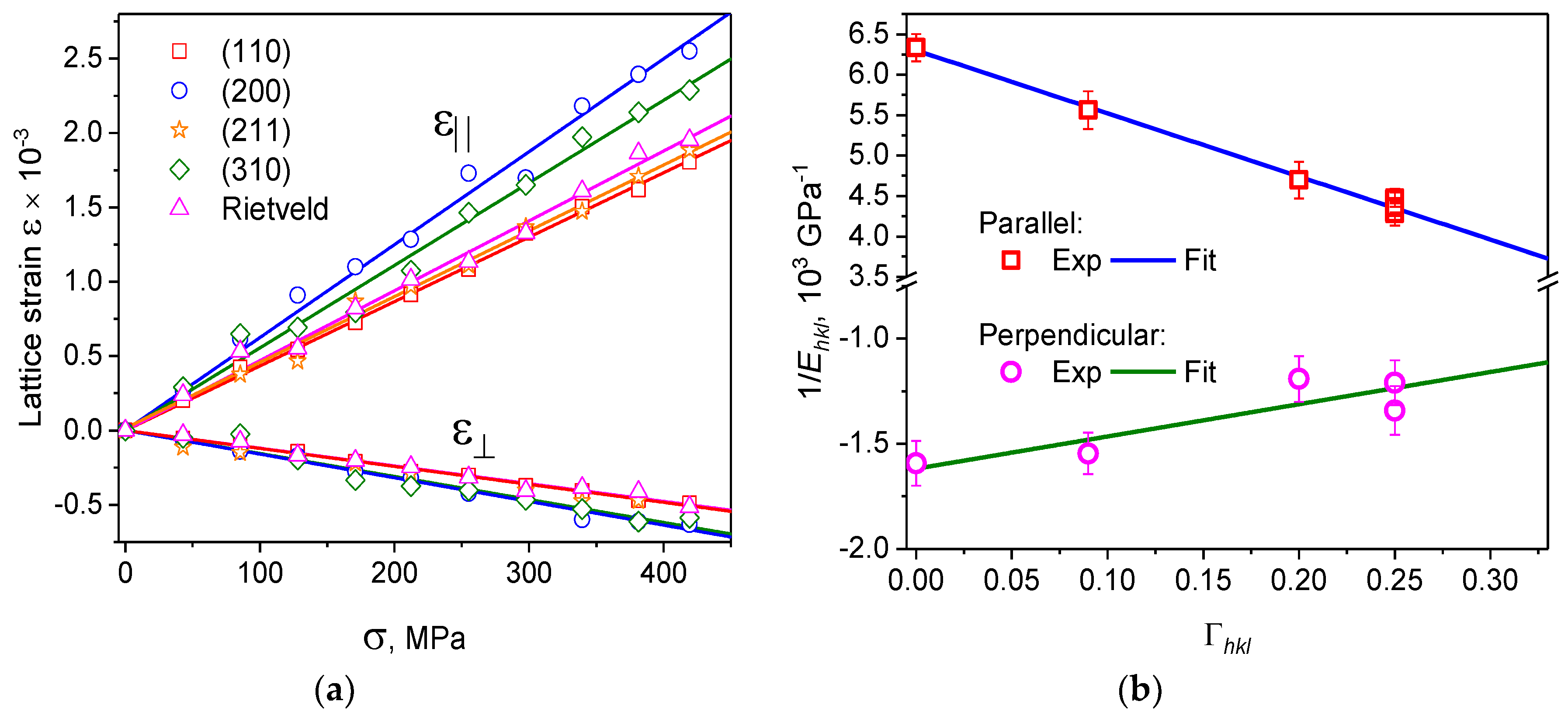
One more application of the TOF neutron diffraction is the in situ study of the behavior of promising materials (composites, gradient materials, steels, alloys, ceramics, etc.) under various conditions (external load, temperature). Typically, the interaction of several phases in a material and their joint effect on the elastic properties and residual stresses are studied. The results of investigations are important for designing new materials with the required physical, chemical, and mechanical properties. As a rule, in such experiments, a sample of investigated material undergoes uniaxial tension or compression in a special loading device directly in a neutron beam. Using detectors at scattering angles of 2θ = ± 90°, diffraction spectra at specified values of applied load are registered. Thus, two independent strain components are measured at two different orientations of the sample: in the direction of the external load, parallel and perpendicular to the neutron scattering vector Q. Using the TOF method, the strains of all observed reflections hkl are determined from the relative shifts of the diffraction peaks. Usually, in the elastic strain regions, a linear dependence of the lattice strain on the applied load is observed [19,20]. At the same time, the lattice strain exhibits an anisotropic character: εhkl ~ Γhkl, where h, k, and l are the Miller indices, and Γhkl = (h2k2 + h2l2 + k2l2)/(h2 + k2 + l2)2 is the orientation (anisotropy) factor (Figure 18a). In the elastic strain range, one can determine from the linear dependences εhkl(σ) the inverse values of Young’s modulus for each crystallographic plane (hkl), which are also linear functions of the orientation factor Γhkl (Figure 18b). The obtained dependences can be used to estimate the elastic stiffness constants C11, C12, and C44 of the material in terms of the chosen elasticity model (Reuss, Hill, Kröner) and calculate Young’s modulus and the Poisson’s ratio for any crystallographic direction [hkl].
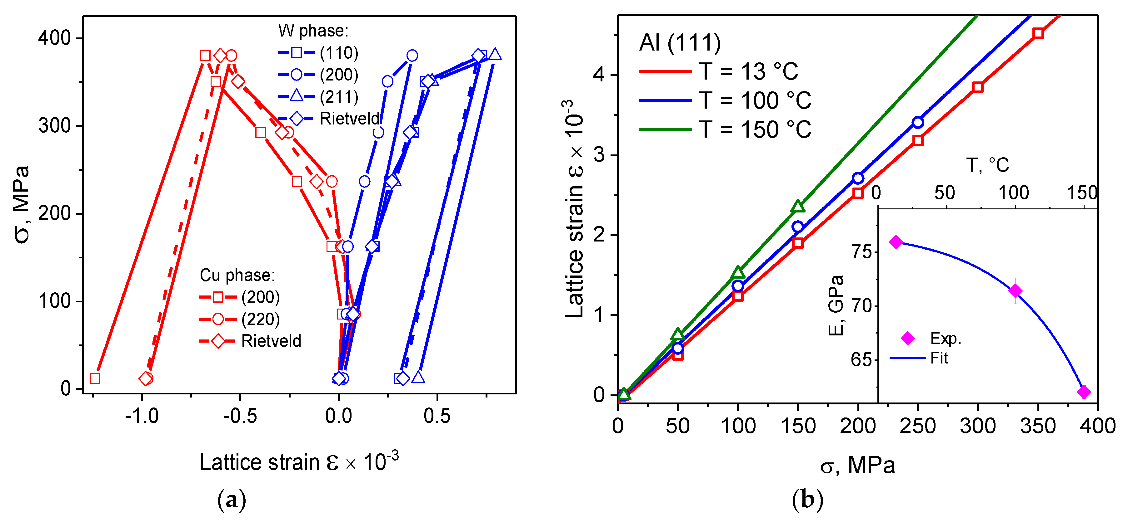
An obvious advantage of neutron time-of-flight diffraction is the wide range of the interplanar spacing with the possibility to observe a set of diffraction peaks simultaneously. This makes it possible to study polycrystalline materials with a rather complex structure, including multiphase materials, in a fixed geometry under various external conditions. In earlier studies [43,44] of W/Cu-graded composite materials, it was shown that the samples prepared by the powder sintering method demonstrate a relatively low level of residual stresses. However, they have a greater brittleness compared with samples prepared by the infiltration method, which limits the prospects of their application. The samples prepared by the infiltration method have a higher level of stresses between phases and better mechanical characteristics. The determining role in the residual stress distribution is played by cooling conditions after fabrication, while the gradient profile proves to be a secondary factor. In continuation of these studies, the redistribution of the load at uniaxial compression between the “hard” and “soft” phases and the anisotropy of the crystal lattice strain in the homogeneous (with no gradient) composite material W/Cu prepared by the infiltration method were investigated (Figure 19a) [19]. Analysis of the diffraction reflection intensities showed that the copper phase demonstrates a moderate texture, whereas in the tungsten phase, a texture is practically absent. From the results of experiments, it was established that in the tungsten phase up to ~350 MPa, the strain is elastic, while in the copper phase, plastic deformation starts from ~85 MPa Thus, the redistribution of the main load occurs into the plastically deformed copper phase upon the slight growth of strains in tungsten.
Eхtended possibilities for studying the thermal and mechanical properties of materials arise when neutron diffraction experiments are performed in situ with a combination of external load and high temperature [19]. Thus, for widespread D16 aluminum alloy, degradation of the elastic properties of the material was studied at various temperatures (Figure 19b). The precision of determining the lattice strain on the FSD diffractometer turned out to be high enough, which made it possible to reliably observe the difference between ε(σ) curves at different temperatures and estimate the changes in the elastic properties of the material as a function of temperature. The results of experiments revealed that in the temperature range 13–150 °C, the modulus of elasticity of the material steadily decreases from 76 to 62 GPa. A similar temperature dependence was also observed for the ultimate strength of the material.
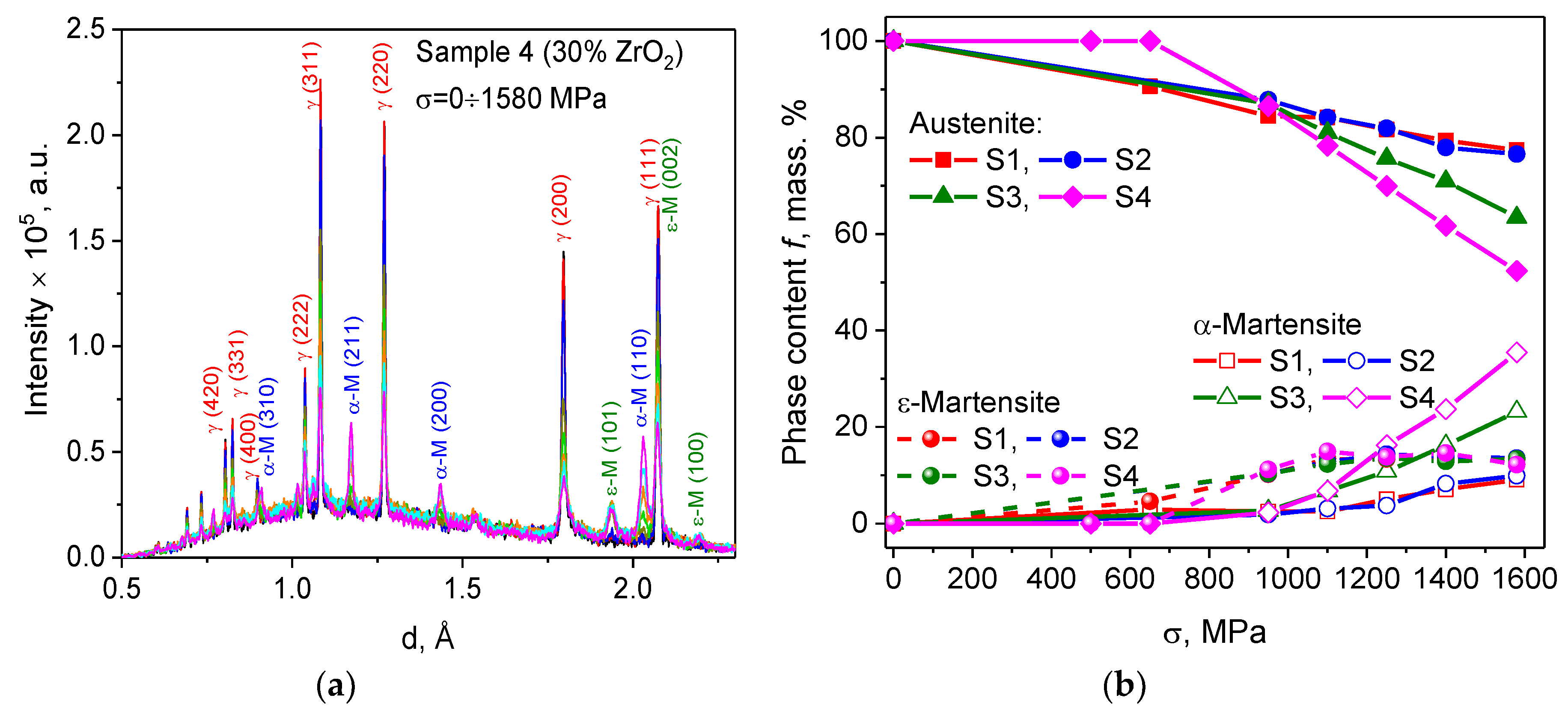
In recent experiments [45] on FSD, the main parameters of the microstructure of TRIP composites with an austenitic matrix and a ZrO2 zirconium-dioxide reinforcing phase subjected to plastic deformation of different degrees were investigated. Two series of samples of the TRIP composite with an austenitic matrix and a strengthening phase of zirconium dioxide ZrO2, partly stabilized by magnesium (Mg-PSZ, series 1) and by yttrium dioxide (Y-PSZ, series 2), were prepared by the powder metallurgy method using hot pressing. In each series, the content of the ZrO2 ceramic phase was 0, 10, 20, 30, and 100 wt % and the samples were designated, respectively, as S1, S2, S3, S4, and S5. The samples of series 1 underwent plastic deformation in ex situ experiments by means of uniaxial compression at different loads: σ = 0, 500, 650, 800, 950, 1100, 1250, 1400, and 1580 MPa. After each deformation cycle, the load was removed and the diffraction spectra of the deformed sample were measured. The samples of series 2 were investigated in in situ experiments, during which they were subjected to uniaxial tension/compression up to destruction in loading machine LM-29 directly in the neutron beam.
In the plasticity region at a load above 650 MPa, the formation of two martensitic phases was observed in the austenitic matrix of series 1 samples: the cubic α’-martensite (space group ) and the hexagonal ε-martensite (space group P63/mmc) (Figure 20a). The phase distribution by Rietveld analysis is shown in Figure 20b. In the ceramic sample S5 of pure zirconium dioxide (100% ZrO2), two phases were observed: cubic (f ≈ 55%) and tetragonal (f ≈ 45%). The ratio between the phases was practically unchanged with an increasing degree of plastic deformation. In addition, in the plasticity region, a considerable anisotropic broadening of the diffraction peak was observed. The anisotropy of peak broadening is due to the elastic fields of dislocations in the material and, correspondingly, a variation in the dislocation contrast factor at the neutron or X-ray scattering [42]. Thus, the estimated dislocation densities for the austenitic matrix demonstrate similar dependences for all samples. The maximum values of dislocation density lie in the range (12 ÷ 20) × 1014 m−2, depending on the zirconium dioxide content in the composite.
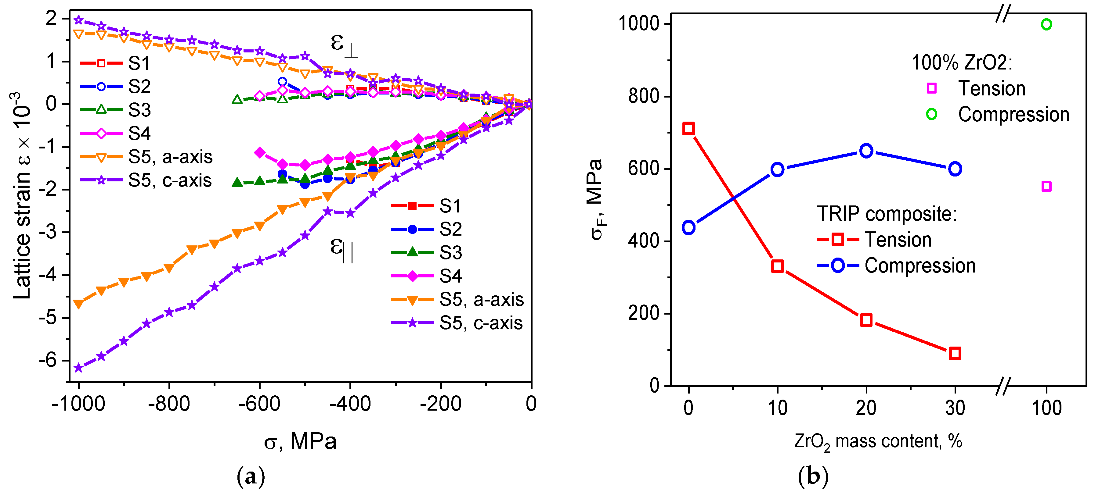
Strain-stress curves were measured during in situ neutron experiments with series 2 samples (Figure 21a). The Young’s modulus and the Poisson ratio determined from the linear dependences ε(σ) in the elastic region demonstrate a strong dependence on the zirconium dioxide content and a considerable difference in their values for compression and tension. The similar dependence on the zirconium dioxide content was also observed for the ultimate strength of the material (Figure 21b). Probably, the main factor explaining such behavior of the material is the formation of microcracks at the interphase boundaries during the deformation process. Further, the small stress jumps, observed on the strain-stress curves, are additional evidence in favor of this hypothesis.
The behavior of the austenitic matrix in the plastic deformation region is similar to that observed in the series 1 with nearly the same level of dislocation density in the material. The martensitic phase formation in sample S1 (pure austenitic matrix) started from loads of 350 MPa and higher, while no martensitic phase formation was observed for samples S2–S4. Apparently, the reason for such a behavior is load redistribution between the austenitic phases and ZrO2 ceramics and the formation of microcracks at the interphase boundaries, due to which the load level in the austenitic matrix did not attain values sufficient for phase transformations.
5. Conclusions
Accumulated work experience has shown that the correlation RTOF diffractometry at a long-pulse neutron source possesses many advantages and, therefore, can be considered as a suitable tool for residual stress investigations in bulk samples and for the precise characterization of the microstructure of modern structural materials. The achieved high resolution level at a relatively short flight path allows investigating important parameters of materials’ microstructure, such as lattice strain, microstrain, and size of crystallites. At present, the regular experiments for residual stress and microstrain studies in bulk industrial components and in new advanced materials are successfully performed on the FSD diffractometer.
Further development of the FSD diffractometer will include an upgrade and expansion of the detector system: 14 new TOF focused ZnS(Ag) elements will be installed in the near future on both (right and left) banks of 90°-detectors, which will increase the scattering angle range by up to 40° for each detector. The spectral distribution of the incident neutron beam will be optimized by installing a new supermirror-coated neutron guide. Another important task is the replacement of the Fourier chopper. Currently, a new Fourier chopper is being developed that operates in a vacuum and has improved dynamic characteristics. This device is a rotor-stator system with real cut-away radial slits and 10B absorbing layers. As the source of the pickup signal, it is supposed to use a laser beam passing through the chopper slits. Such design of the new chopper provides more precise PID control, no phase error (shift of pickup signal phase with respect to the neutron signal), no absorption and scattering from the chopper disc material, less vibration, and gamma background. Thus, all these developments can significantly enhance the quality of the diffraction spectrum, i.e., reduce the background, increase the intensity of the spectrum, and improve the profile and symmetry of the diffraction peak.
Funding
At the initial stage of FSD construction, the work was financed within FLNP JINR Topical Research Plan. The development of FSD was partially supported within the JINR–BMBF (Germany), JINR-Romania, JINR-Poland cooperation projects as well as within projects of the Russian Foundation for Basic Research (grants No. 14-42-03585_r_center_a and 15-08-06418_a.)
Acknowledgments
The author is grateful to A.M. Balagurov, V.V. Zhuravlev, P. Petrov and S.V. Guk for useful discussions. The author is in debt to I.V. Papushkin for experimental assistance.
Conflicts of Interest
The author declares no conflict of interest.
References
- Colwell, J.F.; Lehinan, S.R.; Miller, P.H., Jr.; Whittemore, W.L. Fourier analysis of thermal neutron time-of-flight data: A high efficiency neutron chopping system, I. Nucl. Instrum. Methods 1969, 76, 135–149. [Google Scholar] [CrossRef]
- Colwell, J.F.; Lehinan, S.R.; Miller, P.H., Jr.; Whittemore, W.L. Fourier analysis of thermal neutron time-of-flight data: A high efficiency neutron chopping system, II. Nucl. Instrum. Methods 1970, 77, 29–39. [Google Scholar] [CrossRef]
- Nunes, A.C.; Nathans, R.; Schoenborn, B.P. A neutron Fourier chopper for single crystal reflectivity measurements: Some general design considerations. Acta Cryst. 1971, 27, 284–291. [Google Scholar] [CrossRef]
- Nunes, A.C. The neutron Fourier chopper in protein crystallography. J. Appl. Crystallogr. 1975, 8, 20–28. [Google Scholar] [CrossRef] [Green Version]
- Pöyry, H.; Hiismäki, P.; Virjo, A. Principles of reverse neutron time-of-flight spectrometry with Fourier chopper applications. Nucl. Instrum. Methods 1975, 126, 421–433. [Google Scholar] [CrossRef]
- Tiitta, A.; Hiismäki, P. ASTACUS, a time focussing neutron diffractometer based on the reverse Fourier principle. Nucl. Instrum. Methods 1979, 163, 427–436. [Google Scholar] [CrossRef]
- Antson, O.K.; Bulkin, A.; Hiismäki, P.; Korotkova, T.; Kudryashev, A.; Kukkonen, H.; Muratov, V.; Pöyry, H.; Schebetov, A.; Tiita, A. High-resolution Fourier TOF powder diffraction: I. Performance of the “mini-sfinks” facility. Phys. B Conden. Matter 1989, 156, 567–570. [Google Scholar] [CrossRef]
- Schröder, J.; Kudryashev, V.A.; Keuter, J.M.; Priesmeyer, H.G.; Larsen, J.; Tiitta, A. FSS-a novel RTOF-diffractometer optimized for residual stress investigations. J. Neutron Res. 1994, 2, 129–141. [Google Scholar] [CrossRef]
- Priesmeyer, H.G.; Larsen, J.; Meggers, K. Neutron diffraction for non-destructive strain/stress measurements in industrial devices. J. Neutron Res. 1994, 2, 31–52. [Google Scholar] [CrossRef]
- Hiismäki, P.; Pöyry, H.; Tiitta, A. Exploitation of the Fourier chopper in neutron diffractometry at pulsed sources. J. Appl. Crystallogr. 1988, 21, 349–354. [Google Scholar] [CrossRef] [Green Version]
- Balagurov, A.M. Scientific Reviews: High-resolution fourier diffraction at the ibr-2 reactor. Neutron News 2005, 16, 8–12. [Google Scholar] [CrossRef]
- Balagurov, A.M.; Bobrikov, I.A.; Bokuchava, G.D.; Zhuravlev, V.V.; Simkin, V.G. Correlation Fourier diffractometry: 20 years of experience at the ibr-2 reactor. Phys. Part. Nuclei 2015, 46, 249–276. [Google Scholar] [CrossRef]
- Balagurov, A.M.; Bokuchava, G.D.; Schreiber, J.; Taran, Y.V. Equipment for residual stress measurements with the high resolution Fourier diffractometer: Present status and prospects. Mater. Sci. Forum 1996, 228, 265–268. [Google Scholar] [CrossRef]
- Aksenov, V.L.; Balagurov, A.M.; Bokuchava, G.D.; Schreiber, J.; Taran, Y.V. Estimation of residual stress in cold rolled iron-disks using magnetic and ultrasonic methods and neutron diffraction technique. MRS Proc. 1995, 376, 415–421. [Google Scholar] [CrossRef]
- Balagurov, A.M.; Bokuchava, G.D.; Schreiber, J.; Taran, Y.V. Neutron diffraction investigations of stresses in austenitic steel. Phys. B 1997, 234, 967–968. [Google Scholar] [CrossRef]
- Kockelmann, H.; Bokuchava, G.D.; Schreiber, J.; Taran, Y.V. Measurements of residual stresses in a shape welded steel tube by neutron and X-ray diffraction. Textures Microstruct. 1999, 33, 231–242. [Google Scholar] [CrossRef]
- Bokuchava, G.D.; Aksenov, V.L.; Balagurov, A.M.; Zhuravlev, V.V.; Kuzmin, E.S.; Bulkin, A.P.; Kudryashev, V.A.; Trounov, V.A. Neutron Fourier diffractometer FSD for internal stress analysis: First results. Appl. Phys. A 2002, 74 (Suppl. 1), 86–88. [Google Scholar] [CrossRef]
- Allen, A.J.; Hutchings, M.T.; Windsor, C.G.; Andreani, C. Neutron diffraction methods for the study of residual stress fields. Adv. Phys. 1985, 34, 445–473. [Google Scholar] [CrossRef]
- Bokuchava, G.D.; Papushkin, I.V. Neutron time-of-flight stress diffractometry. J. Surf. Investig. X-Ray Synchrotron Neutron Tech. 2018, 12, 97–102. [Google Scholar] [CrossRef]
- Bokuchava, G.D. Materials microstructure characterization using high resolution time-of-flight neutron diffraction. Rom. J. Phys. 2016, 61, 903–925. [Google Scholar]
- Bokuchava, G.D.; Papushkin, I.V.; Bobrovskii, V.I.; Kataeva, N.V. Evolution in the dislocation structure of austenitic 16Cr–15Ni–3Mo–1Ti steel depending on the degree of cold plastic deformation. J. Surf. Investig. X-Ray Synchrotron Neutron Tech. 2015, 9, 44–52. [Google Scholar] [CrossRef]
- Balagurov, A.M.; Bobrikov, I.A.; Bokuchava, G.D.; Vasin, R.N.; Gusev, A.I.; Kurlov, A.S.; Leoni, M. High-resolution neutron diffraction study of microstructural changes in nanocrystalline ball-milled niobium carbide NbC0.93. Mater. Charact. 2015, 109, 173–180. [Google Scholar] [CrossRef]
- Hiismäki, P. Modulation Spectrometry of Neutrons with Diffractometry Applications; World Scientific: Singapore, 1997. [Google Scholar]
- Balagurov, A.M.; Bokuchava, G.D.; Kuzmin, E.S.; Tamonov, A.V.; Zhuk, V.V. Neutron RTOF diffractometer FSD for residual stress investigation. Z. Kristallog Suppl. Issue 2016, 23, 217–222. [Google Scholar]
- Bokuchava, G.D.; Balagurov, A.M.; Sumin, V.V.; Papushkin, I.V. Neutron Fourier diffractometer FSD for residual stress studies in materials and industrial components. J. Surf. Investig. X-Ray Synchrotron Neutron Tech. 2010, 4, 879–890. [Google Scholar] [CrossRef]
- Bogdzel, A.A.; Bokuchava, G.D.; Butenko, V.A.; Drozdov, V.A.; Zhuravlev, V.V.; Kuzmin, E.S.; Levchanovskii, F.V.; Pole, A.V.; Prikhodko, V.I.; Sirotin, A.P. system for automation of experiments on neutron Fourier diffractometer FSD. In Proceedings of the XIX International Symposium “Nuclear Electronics & Computing” (NEC'2003), Varna, Bulgaria, 15–20 September 2003. [Google Scholar]
- Carpenter, J.M. Extended detectors in neutron time-of-flight diffraction experiments. Nucl. Instrum. Methods 1967, 47, 179–180. [Google Scholar] [CrossRef]
- Kudryashev, V.A.; Trounov, V.A.; Mouratov, V.G. Improvement of Fourier method and Fourier diffractometer for internal residual strain measurements. Phys. B 1997, 234, 1138–1140. [Google Scholar] [CrossRef]
- Kuzmin, E.S.; Balagurov, A.M.; Bokuchava, G.D.; Zhuk, V.V.; Kudryashev, V.A. Detector for the FSD Fourier diffractometer based on ZnS (Ag)/6LiF scintillation screen and wavelength shifting fiber readout. J. Neutron Res. 2002, 10, 31–41. [Google Scholar] [CrossRef]
- Bokuchava, G.D.; Papushkin, I.V.; Tamonov, A.V.; Kruglov, A.A. Residual stress measurements by neutron diffraction at the IBR-2 pulsed reactor. Rom. J. Phys. 2016, 61, 491–505. [Google Scholar]
- Webster, G.A. Neutron Diffraction Measurements of Residual Stress in A Shrink-Fit Ring and Plug; National Physical Laboratory: Middlesex, UK, 2000. [Google Scholar]
- Murashkevich, S.M.; Levchanovskiy, F.V. A data acquisition system for neutron spectrometry: The new approach and the implementation. In Proceedings of the XXIV International Symposium. “Nuclear Electronics & Computing” (NEC’2013), Varna, Bulgaria, 9–16 September 2013. [Google Scholar]
- Mouratov, V.G.; Pirogov, A.M. Multidetector RTOF analyzer. Phys. B 1997, 234, 1099–1101. [Google Scholar] [CrossRef]
- Genchev, G.; Doynov, N.; Ossenbrink, R.; Michailov, V.; Bokuchava, G.; Petrov, P. Residual stresses formation in multi-pass weldment: A numerical and experimental study. J. Constr. Steel Res. 2017, 138, 633–641. [Google Scholar] [CrossRef]
- Rietveld, H.M. A profile refinement method for nuclear and magnetic structures. J. Appl. Crystallogr. 1969, 2, 65–71. [Google Scholar] [CrossRef] [Green Version]
- Petrov, P.I.; Bokuchava, G.D.; Papushkin, I.V.; Genchev, G.; Doynov, N.; Michailov, V.G.; Ormanova, M.A. Neutron diffraction studies of laser welding residual stresses. Proc. SPIE 2017. [Google Scholar] [CrossRef]
- Bokuchava, G.; Papushkin, I.; Petrov, P. Residual Stress Study by Neutron Diffraction in the Charpy Specimens Reconstructed by Various Welding Methods. C. R. Acad. Bulg. Sci. 2014, 67, 763–768. [Google Scholar]
- Bokuchava, G.D.; Petrov, P.; Papushkin, I.V. Application of Neutron Stress Diffractometry for Studies of Residual Stresses and Microstrains in Reactor Pressure Vessel Surveillance Specimens Reconstituted by Beam Welding Methods. J. Surf. Investig. X-Ray Synchrotron Neutron Tech. 2016, 10, 1143–1153. [Google Scholar] [CrossRef]
- Radaj, D. Heat Effects of Welding. Temperature Field, Residual Stress, Distortion; Springer: Berlin, Germany, 1992. [Google Scholar]
- Warren, B.E.; Averbach, B.L. The Effect of Cold-Work Distortion on X-Ray Patterns. J. Appl. Crystallogr. 1950, 21, 595–599. [Google Scholar] [CrossRef]
- Ungár, T.; Tichy, G. The Effect of Dislocation Contrast on X-Ray Line Profiles in Untextured Polycrystals. Phys. Status Solidi A 1999, 171, 425–434. [Google Scholar] [CrossRef]
- Ungár, T.; Dragomir, I.; Révész, Á.; Borbély, A. The contrast factors of dislocations in cubic crystals: The dislocation model of strain anisotropy in practice. J. Appl. Crystallogr. 1999, 32, 992–1002. [Google Scholar] [CrossRef]
- Bokuchava, G.D.; Schreiber, J.; Shamsutdinov, N.; Stalder, M. Residual stress studies in graded W/Cu materials by neutron diffraction method. Phys. B 2000, 276, 884–885. [Google Scholar] [CrossRef]
- Bokuchava, G.D.; Schreiber, J.; Shamsutdinov, N.; Stalder, M. Residual stress states of graded CuW materials. Mater. Sci. Forum 1999, 308, 1018–1023. [Google Scholar] [CrossRef]
- Bokuchava, G.D.; Gorshkova, Y.E.; Papushkin, I.V.; Guk, S.; Kawalla, R. Investigation of plastically deformed TRIP composites by neutron diffraction and small angle neutron scattering methods. J. Surf. Investig. X-ray Synchrotron Neutron Tech. 2018, 12, 227–232. [Google Scholar] [CrossRef]
Figure 1.
(a) Experimental layout for residual stress scanning in a bulk object. Incident and scattered neutron beams are restricted by a diaphragm and radial collimators shaping a gauge volume within the specimen; (b) Visualization of diffraction peak (110) shift at stress values of 20, 100, and 200 MPa observed at the diffractometer with a resolution level of R = Δd/d ≈ 0.001 (ferritic steel, E ≈ 200 GPa).

Figure 2.
Typical dependences of Δd2(d2) demonstrating contributions to the diffraction peak width due to isotropic microstrain ε (straight line) and crystallite size 〈D〉 (parabolic dependence).
Figure 2.
Typical dependences of Δd2(d2) demonstrating contributions to the diffraction peak width due to isotropic microstrain ε (straight line) and crystallite size 〈D〉 (parabolic dependence).

Figure 3.
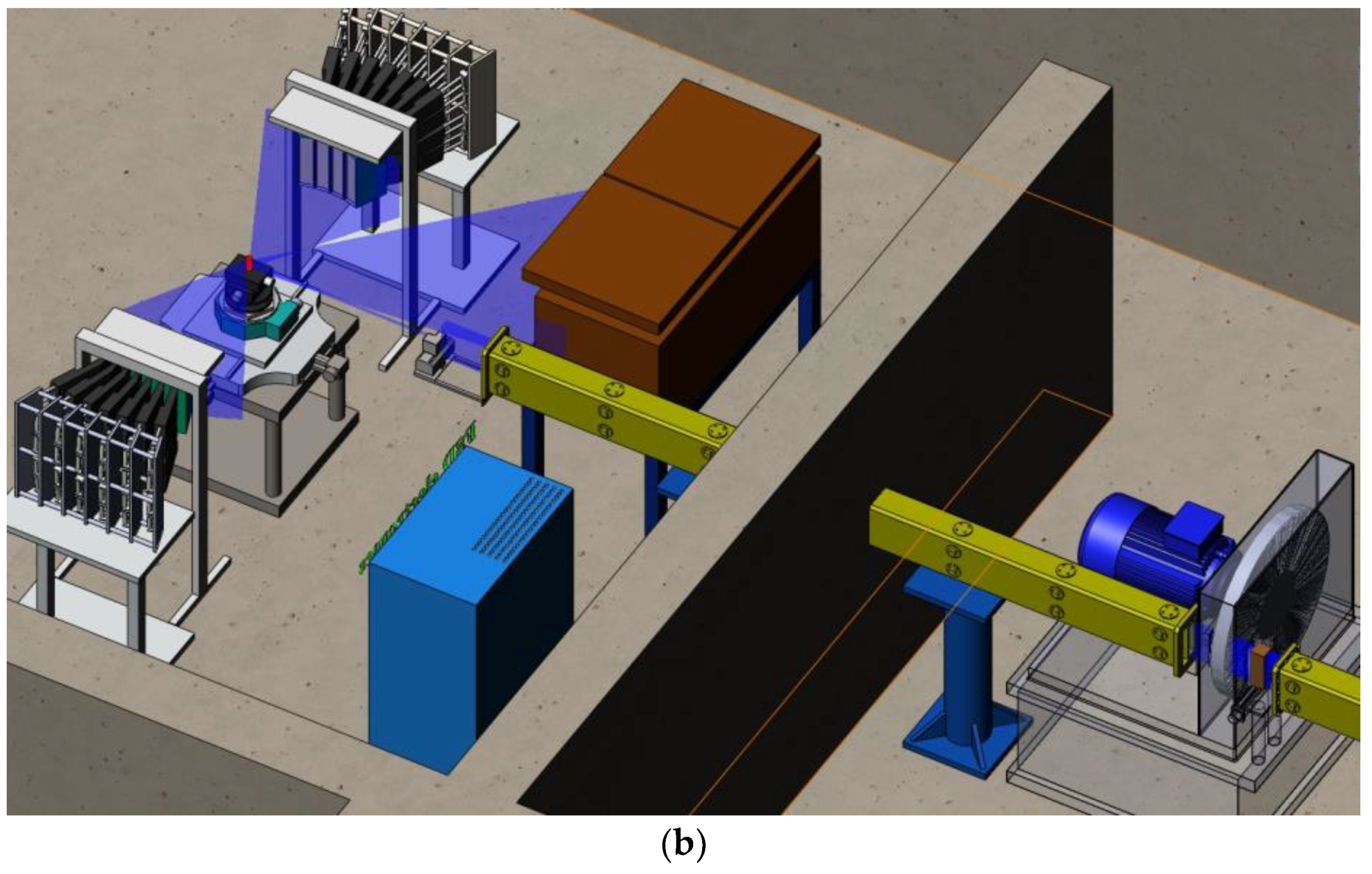
(a) Layout of the FSD diffractometer (Fourier Stress Diffractometer) at the IBR-2 pulsed reactor (FLNP JINR, Dubna); (b) 3D model of the FSD diffractometer. The basic functional units of the FSD are the long mirror neutron guide with variable diaphragms, the fast Fourier chopper, the detector system consisting of ±90°-detectors with radial collimators and a backscattering detector, the HUBER goniometer at the sample position, and auxiliary equipment (furnaces, loading machines, etc.), adapted from [25], with permission from © 2010 Springer.
Figure 3.
(a) Layout of the FSD diffractometer (Fourier Stress Diffractometer) at the IBR-2 pulsed reactor (FLNP JINR, Dubna); (b) 3D model of the FSD diffractometer. The basic functional units of the FSD are the long mirror neutron guide with variable diaphragms, the fast Fourier chopper, the detector system consisting of ±90°-detectors with radial collimators and a backscattering detector, the HUBER goniometer at the sample position, and auxiliary equipment (furnaces, loading machines, etc.), adapted from [25], with permission from © 2010 Springer.


Figure 4.
(a) Design of the Fourier chopper, consisting of a rotating rotor disk and a stationary stator. Outer circumference of the rotor disk is a system of interleaving slits transparent and opaque for thermal neutrons. The diagram below shows a saw tooth function of transmission of such a chopper system and its approximating sequence of positive and negative binary (pickup) signals; (b) Photo of the Fourier chopper installed on FSD.

Figure 5.
(a) Arrangement of sensitive ZnS(Ag) scintillator layers of the multi-element ASTRA 90°-detector in the horizontal scattering plane; (b) 3D model of the ASTRA 90°-detector, adapted from [25], with permission from © 2010 Springer.
Figure 5.
(a) Arrangement of sensitive ZnS(Ag) scintillator layers of the multi-element ASTRA 90°-detector in the horizontal scattering plane; (b) 3D model of the ASTRA 90°-detector, adapted from [25], with permission from © 2010 Springer.

Figure 6.
(a) Detector system of the FSD diffractometer, adapted from [25], with permission from © 2010 Springer; (b) Time-focused backscattering detector BS (shielding is removed).
Figure 6.
(a) Detector system of the FSD diffractometer, adapted from [25], with permission from © 2010 Springer; (b) Time-focused backscattering detector BS (shielding is removed).

Figure 7.
(a) Sample place at the FSD diffractometer. Huber goniometer, the diaphragm at the incident beam, and two radial collimators at the scattered beams are visible, adapted from [19], with permission from © 2018 Springer; (b) Calculated transmission map for the new wide-aperture radial collimator.

Figure 8.
(a) Residual lattice strain measured in VAMAS shrink-fit ring and plug sample (set #1); (b) Sample surface scan using a radial collimator: diffraction peak intensity vs. gauge volume position in the material depth, adapted from [25], with permission from © 2010 Springer.
Figure 8.
(a) Residual lattice strain measured in VAMAS shrink-fit ring and plug sample (set #1); (b) Sample surface scan using a radial collimator: diffraction peak intensity vs. gauge volume position in the material depth, adapted from [25], with permission from © 2010 Springer.

Figure 9.
(a) RTOF neutron diffraction spectra measured from a standard α-Fe powder sample with the maximal Fourier chopper speed Ωmax = 4000 rpm. At the bottom, “positive” I+(t) and “negative” I–(t) correlation spectra are shown. The upper pattern is the high-resolution diffraction RTOF spectrum calculated as a difference of “positive” and “negative” patterns: H(t) = I+(t) − I–(t); (b) Diffraction peak (211) region in the same RTOF spectra.

Figure 10.
(a) Diffraction spectra from individual elements of the ASTRA detector; (b) Diffraction spectra from individual elements of the ASTRA detector, reduced to a unified TOF scale and the final total spectrum.
Figure 10.
(a) Diffraction spectra from individual elements of the ASTRA detector; (b) Diffraction spectra from individual elements of the ASTRA detector, reduced to a unified TOF scale and the final total spectrum.

Figure 11.
Neutron diffraction patterns measured from the α-Fe standard sample using BS (a) and 90°-detector ASTRA; (b) at the maximal Fourier chopper speed Ωmax = 6000 rpm. The measured data points, full profile calculated by the Rietveld method, and the difference curve are shown, adapted from [25], with permission from © 2010 Springer.

Figure 12.
(a) FSD resolution function measured at maximal Fourier chopper speed Ωmax = 6000 rpm for backscattering detector BS (2θ = 140°) and both ASTRA detectors (2θ = ± 90°). (b) Diffraction peak shape dependence vs. maximal Fourier chopper speed Vmax, adapted from [25], with permission from © 2010 Springer.

Figure 13.
(a) Four-axis HUBER goniometer for precise sample positioning (max. load 300 kg); (b) Additional goniometer head with ±15°-tilt; (c) Uniaxial mechanical loading machine LM-29 (Fmax = 29 kN, Tmax = 800 °C) installed on the HUBER goniometer during the experiment; (d) Water-cooled mirror furnace (P = 1 kW, Tmax = 1000 °C). A sample with a thermocouple heated during the experiment is shown.

Figure 14.
(a) Multi-pass butt-welded (GMAW+SAW) specimen (300 × 100 × 20 mm3). (b) Longitudinal σX and transverse σY stress distribution in a multi-pass butt-welded joint measured by neutron diffraction and calculated by FEM, adapted from [34], with permission from © 2017 Elsevier.
Figure 14.
(a) Multi-pass butt-welded (GMAW+SAW) specimen (300 × 100 × 20 mm3). (b) Longitudinal σX and transverse σY stress distribution in a multi-pass butt-welded joint measured by neutron diffraction and calculated by FEM, adapted from [34], with permission from © 2017 Elsevier.

Figure 15.
Residual strain (a) and stress (b) measured by neutron diffraction and FEM calculations for thin steel plate sample with a laser beam welded (LBW) joint. (c) Dislocation density distribution estimated from diffraction peak broadening in the LBW sample, adapted from [36], with permission from © 2017 SPIE.

Figure 16.
(a) Residual stress distribution in the test Charpy specimen (LBW2) reconstituted by the laser beam welding technique. Inset: LBW2 Charpy specimen (10 × 10 × 55 mm3) with two weld seams at X = 0 and X = 14 mm, adapted from [38], with permission from © 2016 Springer. (b) Diffraction peak (110) profile fitted with a Voigt function at the weld seam center (X = 9 mm) and in the base material (X = 17 mm).

Figure 17.
(a) Crystallite sizes 〈D〉 vs. scan coordinate X for all studied Charpy specimens. (b) Dislocation density distributions vs. scan coordinate X, adapted from [38], with permission from © 2016 Springer.
Figure 17.
(a) Crystallite sizes 〈D〉 vs. scan coordinate X for all studied Charpy specimens. (b) Dislocation density distributions vs. scan coordinate X, adapted from [38], with permission from © 2016 Springer.

Figure 18.
(a) Longitudinal and transverse lattice strain of ferrite steel vs. applied load for different crystal planes. (b) Inverse values of longitudinal and transverse Young’s moduli vs. anisotropy (orientation) factor Гhkl, adapted from [19], with permission from © 2018 Springer.
Figure 18.
(a) Longitudinal and transverse lattice strain of ferrite steel vs. applied load for different crystal planes. (b) Inverse values of longitudinal and transverse Young’s moduli vs. anisotropy (orientation) factor Гhkl, adapted from [19], with permission from © 2018 Springer.

Figure 19.
(a) Transverse lattice strain for different planes (hkl) of copper and tungsten phases in the W/Cu composite vs. external load. (b) Lattice strain for the (111) plane in the aluminium alloy vs. applied load measured at different temperatures: 13, 100, and 150 °С. Inset: temperature dependence of the elasticity modulus for the aluminium alloy: symbols designate experimental values, with the solid line corresponding to the least square fit E = E0 − B∙T∙exp(−T0/T), adapted from [19], with permission from © 2018 Springer.

Figure 20.
(a) The evolution of the diffraction pattern of TRIP-composite as a function of plastic deformation (sample S4, σ = 0 ÷ 1580 MPa). The Miller indices of the main peaks of austenitic and α’- and ε-martensitic phases are indicated; (b) Mass content of the observed phases vs. plastic deformation degree for all investigated samples, adapted from [45], with permission from © 2018 Springer.

Figure 21.
(a) Longitudinal and transverse lattice strain determined from the relative change in the lattice parameter for the austenitic matrix of the TRIP-composite for samples S1-S4 and for the ceramic sample S5 (100% ZrO2). (b) The ultimate stress of the TRIP composite vs. ZrO2 content, adapted from [45], with permission from © 2018 Springer.


Table 1.
Main parameters of the FSD diffractometer.
| Curved Neutron Guide: | Mirror with Ni Coating |
| length | 19 m |
| curvature radius | 2864.8 m |
| Straight neutron guide: | Mirror with Ni Coating |
| length | 5.01 m |
| Neutron beam size at the sample position (variable) | (0 ÷ 10) × (0 ÷ 75) mm |
| Moderator–sample distance | 28.14 m |
| Chopper–sample distance | 5.55 m |
| Fourier chopper (Disk): | High-strength Al Alloy |
| outer diameter | 540 mm |
| single slit width | 0.7 mm |
| number of slits | 1024 |
| maximum speed of rotation | 6000 rpm |
| maximum frequency of neutron beam modulation | 102.4 kHz |
| Thermal Neutron Pulse Width: | Water Moderator |
| in the low-resolution mode (TOF) | 340 µs |
| in the high-resolution mode (RTOF) | 9.8 µs |
| Neutron flux at the sample position: | |
| without Fourier chopper | 1.8 × 10⁶ neutron/cm2⋅sec |
| with Fourier chopper | 3.7 × 10⁵ neutron/cm2⋅sec |
| Wavelength range | 0.9 ÷ 8 Å |
| Detectors: | |
| 2θ = 140° (backscattering) | 6Li, with geometrical TOF focusing |
| 2θ = ± 90° | ZnS(Ag), with combined electronic and geometrical TOF focusing |
| Detector resolution Δd/d (at d = 2 Å): | |
| 2θ = 140° (backscattering) | 2.3 × 10⁻³ |
| 2θ = ± 90° | 4.0 × 10⁻³ |
| dhkl range: | |
| 2θ = 140° (backscattering) | 0.51 ÷ 5.39 Å |
| 2θ = ± 90° | 0.63 ÷ 6.71 Å |
© 2018 by the author. Licensee MDPI, Basel, Switzerland. This article is an open access article distributed under the terms and conditions of the Creative Commons Attribution (CC BY) license (http://creativecommons.org/licenses/by/4.0/).
Share and Cite
MDPI and ACS Style
Bokuchava, G. Neutron RTOF Stress Diffractometer FSD at the IBR-2 Pulsed Reactor. Crystals 2018, 8, 318. https://doi.org/10.3390/cryst8080318
AMA Style
Bokuchava G. Neutron RTOF Stress Diffractometer FSD at the IBR-2 Pulsed Reactor. Crystals. 2018; 8(8):318. https://doi.org/10.3390/cryst8080318
Chicago/Turabian StyleBokuchava, Gizo. 2018. "Neutron RTOF Stress Diffractometer FSD at the IBR-2 Pulsed Reactor" Crystals 8, no. 8: 318. https://doi.org/10.3390/cryst8080318
Note that from the first issue of 2016, this journal uses article numbers instead of page numbers. See further details here.