Polymer-Optical-Fiber Lasers and Amplifiers Doped with Organic Dyes


Abstract
: Polymer optical fibers (POFs) doped with organic dyes can be used to make efficient lasers and amplifiers due to the high gains achievable in short distances. This paper analyzes the peculiarities of light amplification in POFs through some experimental data and a computational model capable of carrying out both power and spectral analyses. We investigate the emission spectral shifts and widths and on the optimum signal wavelength and pump power as functions of the fiber length, the fiber numerical aperture and the radial distribution of the dopant. Analyses for both step-index and graded-index POFs have been done.1. Introduction
Polymer optical fibers (POFs), due to their flexibility and ease of use, have very interesting characteristics for short-haul communication links, as well as for other applications in fields such as optical sensing, illumination and passive optical devices [1]. In addition, they constitute a promising research field as active devices, in combination with organic dopants (either organic dyes or organic semiconductors). The aim is to achieve efficient fiber lasers and amplifiers, and even optical-gain switches [2-6], in short fiber distances. High-gain amplifiers have been reported in distances shorter than 1 m, due to the high emission and absorption cross sections of organic dopants. The probability of light interacting with a molecule of dopant is quantified by the cross section for the relevant type of interaction, for example, absorption or emission. The cross section depends on the wavelength of the light. The total probability of interaction also depends on the concentration of dopant molecules per unit volume. For example, in the case of the dye rhodamine B (RB), the cross sections are about 10,000 times greater than that of Er in glass fibers. Optical amplification in dye-doped POFs was reported for the first time in 1993, for the case of a graded-index (GI) fiber doped with RB [7]. More recently, a preform technique was presented and used to fabricate RB-doped step-index (SI) POFs [6]. The optical feedback for the gain medium in active POFs is usually provided by the cylindrical surface of the optical fiber, which acts as a cavity.
As is well-known, POFs are more suitable than glass fibers for using organic dopants, because of their lower manufacturing temperature as compared to that of glass fibers. Besides, POFs are preferable over other solid hosts because of the higher density of light present in fiber cores, which increases the probability of stimulated emissions. The maximum gain usually takes place near the peak wavelength of the emission cross section [8]. For example, by doping SI or GI POFs with RB and pumping them optically, it is possible to achieve amplification in the visible region. The total gain depends mainly on the dopant concentration, on the fiber characteristics and on the energy of the pump pulses. High gains can be achieved in both SI and GI active POFs, although with some peculiarities that will be reviewed in this paper. The type of POF chosen will also depend on the rest of the optical link used to connect the emitter and the receiver. The main advantage of passive GI POFs is that their bandwidth is typically 2 orders of magnitude larger than that of SI POFs, but they are not so cheap [9].
Organic semiconductors usually yield lower gains than dyes, but they have other interesting properties. For example, whereas dye-doped fiber lasers and amplifiers have to be pumped optically, organic semiconductors open the possibility of electrical pumping in the future, since they are capable of charge transport [10]. In the case of POFs doped with conjugated organic semiconductors, such as the commonly-studied poly(9,9-dioctylfluorene) (PFO), ultrafast-switching capabilities have been observed [5,11]. Specifically, by impinging a second laser pulse at the correct wavelength, the stimulated emission can be annihilated, with almost instantaneous recovery. However, the gains reported so far with PFO and some other fluorine oligomers have been much smaller than those achieved with organic dyes. This is because organic dyes have higher optical cross sections, which allow higher gains, and also because they can usually be dissolved in higher concentrations in poly(methyl-methacrylate) (PMMA), which is the typical material of the core [12]. As will be shown in this paper, the length of a POF-based amplifier can be shortened by dissolving the dopant in high concentrations. By using dyes, large gains can be achieved in very sort fiber distances. For example, experimental gains reported for dye-doped POF amplifiers (POFAs) are 27 dB for a 50-cm RB-doped POF [7] or 18 dB for an 8-cm rhodamine 6G-doped POF [13]. Either longitudinal or lateral optical pumping can be employed [2].
In this paper, we analyze POFs that are pumped longitudinally with short light pulses of several energies. The dye chosen for the analysis is RB. Apart from its particularly large cross sections, it has high photochemical stability, which is important in practice to withstand multiple excitation cycles with a pulsed pump laser [14,15]. Moreover, the photostability achieved with RB-doped POFs is greater than that accomplished with most dyes [16,17]. If high-energy photons are used (as in the proximity of the ultraviolet region), photo bleaching can occur [14], which can limit the maximum energy of the pump pulses for some dyes. This is not the case of RB, which is suitable to obtain high gains in the wavelengths of low attenuation in POFs, from the final part of the green color to the beginning of the red.
The paper is organized as follows. The model describing amplification in active SI and GI fibers is explained and discussed in Section 2. The first issue investigated in Section 3 is the spectral shift of the emission with traveled distance in active POFs, which can be employed for making tunable fiber lasers and amplifiers [18]. As will be shown, when the emission and absorption cross sections overlap significantly, the absorption of the fiber can have a strong influence on the output spectrum, which can present a shift either towards longer or towards shorter wavelengths (i.e., “red shift” or “blue shift” respectively) [8]. This paper clarifies to what extent it is possible to tune the spectral emission of active POFs by changing the fiber length. We also study the influence of the pump power on the output spectrum, with and without signal. In the latter case the light emission process is called Amplified Spontaneous Emission (ASE) [19]. The analysis of the ASE provides information about the wavelengths at which high power is achieved in a POF laser. One of the main novelties of our work is that the spectral study has been made computationally for the first time, as far as we know. After the spectral study, we analyze the influence of the distribution of the dopant concentration and the effect of the numerical aperture in doped GI POFs. Specifically, we pay special attention to the radial distributions of the light power density and of the dopant concentration in the fiber core. The emission features of SI POFs and GI POFs are compared, which allows us to reach conclusions about the influence of the type of fiber. Section 3.2 shows results without input signal (i.e., POF lasers) and Section 3.3 results with signal (i.e., POFAs). All these computational analyses can be very useful at the early design stages of POF lasers and amplifiers.
2. Model
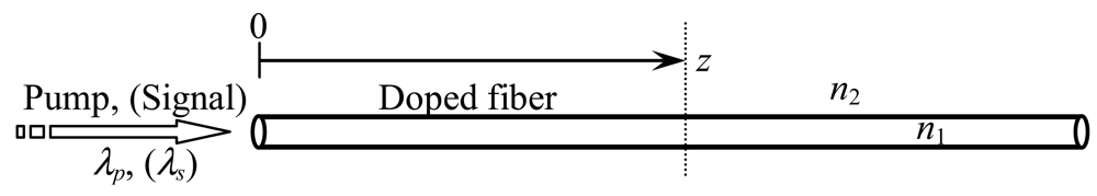
We will start with a brief description of the most important optical transitions that occur in the dopants embedded in the fiber core. As shown in Figure 1, organic dyes have two main electronic energy states, S0 and S1, with many energy vibrational levels within each one of them [20]. Due to the fact that transitions between vibrational levels in each electronic energy state are very rapid and nonradiative, photon emissions are well described as taking place from the ground level of state S1 to one of the vibrational levels of state S0, while photon absorptions are well described as taking place from the ground energy level of state S0 to one of the vibrational levels of state S1. In consequence, the optical properties in the doped fiber are usually analyzed by means of time-dependent rate equations between two main energy levels (from E2 to E1 in Figure 1 for emitted photons) [12].
It is important to note that in our analyses, the independent variables are not only the time t and the position z along the fiber symmetry axis [12], but also the wavelength λ. This allows us to carry out computational simulations of spectral phenomena, such as emission spectral shifts and changes in emission spectral width. To introduce this dependence, we make use of the λ-dependent absorption and emission cross sections σa(λ) and σe(λ) of the dopant, and we divide the range of wavelengths of interest into discrete subintervals centered at wavelengths λk.
We consider that the doped POF is pumped longitudinally at z = 0, with the z axis oriented in the direction of the fiber symmetry axis (see Figure 2). The pump wavelength is λp and the input signal is centered at the wavelength λs.
We assume that the pump laser illuminates the whole cross section of the doped fiber, which, in turn, emits light at random directions. A fraction β of such emissions can propagate towards the output fiber end in guided directions and, therefore, contribute to stimulated emissions along the fiber. β can be calculated from the solid angle corresponding to the maximum inclination with respect to the z axis of guided light rays. For an SI fiber whose core refractive index is n1 and whose cladding refractive index is n2, we can estimate the value of β, which is constant, as the quotient between the solid angle in guided directions and in all directions. In the case of GI fibers, we can first calculate the value of β at the fiber axis (β0) in the same way, as follows:
Additionally, if the dopant concentration and the light density distributions vary with r, which only happens in the case of GI fibers, we have to take the overlapping between both distributions into account. More detailed explanations about this can be found in Appendix. In a typical GI fiber, light is more concentrated towards the fiber symmetry axis, where the dopant concentration is also higher than average. In consequence, stimulated emissions are favored and this effect will be taken into account by means of an overlapping factor γ that will be greater than 1 and which will be explained later. In SI fibers, γ = 1, because the dopant concentration is constant (or also because the light power density is uniform in each fiber cross section).
The complete physical system is described by a set of three partial differential equations with initial and boundary conditions. The unknown functions to be determined are P(t,z,λ) (light power as a function of time, position and wavelength) and N2 (electronic population in the excited level E2). We also take into account the trivial relationship N1 = N−N2 between N2 and the population N1 in level E1, where N is the dopant concentration. The following differential equation governs the evolution of the pump power Pp:
The first right-hand term in Equation (2) represents the absorption of the pump. The product σa(λp) N1 is the absorption coefficient αp of the material at λp. There is an initial increase of N2 due to the pump that reduces N1 and, therefore, it also reduces the absorption coefficient α=N1 σa. The last term in Equation (2) represents the propagation of the pump.
The variation of N2 with time, for each wavelength subinterval centered at λk, is governed by:
The first right-hand term in Equation (3) represents the spontaneous decay, where τ is the spontaneous lifetime of the dopant in PMMA. The second term accounts for the stimulated decay, where σe(λk) is the stimulated emission cross section at λk. Both terms are associated, respectively, with spontaneous and stimulated emissions of photons. The last two terms are associated, respectively, with the absorption of photons of Pp (excitation by the pump) and of P (reabsorption). Reabsorption (the last term) is usually much smaller than excitation by the pump, because P is usually orders of magnitude smaller than Pp and because σa(λp) is larger than σa(λk). Acore is the cross section of the fiber core and h is Planck's constant.
The equation to calculate the evolution of P, for each subinterval centered at λk, is:
The first right-hand term in Equation (4) accounts for the emissions stimulated by incoming photons. The second term represents the attenuation due to material absorption. The third term represents the propagation of the power inside the fiber with speed vz. The last term accounts for the spontaneous emissions, where σspe(λk) is the spontaneous emission cross section at λk, in the sense of determining the probability distribution of the wavelengths of spontaneously emitted photons. More specifically, aspe(λk) is the probability for a spontaneous emission to take place at the wavelength subinterval around λk. Above threshold, the last term in Equation (4), corresponding to spontaneous emissions, tends to be much smaller than the term corresponding to stimulated emissions. However, the former is necessary to simulate the appearance of the first photons in a fiber laser. Note that we have neglected the possible occurrence of absorption of the pump power by excited molecules. The reason is that this phenomenon, which could be important for other applications [21], can be neglected for our type of analysis to a first approach [12]. Besides, in our model we do not include possible nonlinear-absorption effects that could occur at very high power densities, such as the absorption of more than one photon simultaneously or via a multistep process, or the decrease in absorption due to optical saturation or optical bleaching. Such effects would require changing the equations described above. Finally, our model does not take into account modal dispersion in the active POF. However, this approach is reasonable, since the fiber lengths we will work with are very short (no longer than 1 m and even much shorter in some cases).
The aforementioned equations serve for both SI and GI fibers. However, there are two main differences in the values of β and γ in both cases. On the one hand, the overlapping factor γ, which is used in any term in which either P or Pp appears multiplied by N1 or N2, is only different from 1 in GI fibers. On the other hand, an average value of β should be calculated only in GI fibers, so as to take into account that the numerical aperture NA varies with r. In the case of an SI fiber, the numerical aperture is constant along r, so the average value of β in the fiber cross section is simply β0 as in Equation (1). In the case of a GI fiber, the values of β and γ can be calculated in the way shown in Appendix. The results are summarized in Table 1. Depending on the application, GI POFs or SI POFs can be employed, with some differences in gain above threshold of one over another: GI POFs have higher overlapping factors and lower average values of NA. Specifically, in GI POFs there is a decrease in the numerical aperture when r increases, which is a disadvantage over SI POFs regarding the total emitted power, because it implies smaller guided angles of rays and, therefore, fewer guided rays that yield amplification. On the other hand, the dye concentration in GI POFs is maximum at r = 0, where the light density in a GI fiber is also maximum, so γ > 1. This is an advantage of GI over SI fibers. We will show that the greater γ is, the higher the gain of the GI POF tends to be, which is an advantage over SI POFs, for which γ = 1.
The governing differential equations are solved for the following initial conditions: P and N2 are 0 everywhere at t = 0. For the spectral analyses, the powers plotted in the results will represent the time-integrated ones, i.e., . Note that the output power calculated computationally in this uni-dimensional model stands for the total power in a 3-dimensional real fiber with modes.
As for the boundary conditions at z = 0, a Gaussian pulse of pump power is launched, and, in the case of amplifiers, a Gaussian pulse of signal power is added to it, their maxima taking place at the same instant.
The numerical approach used to solve the governing equations relies on finite differences. Specifically, we have developed ad-hoc finite-difference algorithms in which all three variables z, t and λ, have been discretized. The discretization of the spatial and temporal variables is uniform, i.e., with constant finite step sizes δt and δz. For example, for a distance of 7 cm and a pulse width of 5 ns, δz is on the order of 600 ×10−9 m, δt is on the order of 0.2 × 10⁻⁹ s, and roughly 8,000 spatial nodes with at least 200 temporal steps are used. For smaller pulse widths, δt is reduced. The judicious choice of these parameters is critical in order to achieve numerical convergence within the desired precision. The number of discrete wavelength subintervals is not so critical for convergence, and it is has been on the order of 50 in most of our simulations.
As for the implementation of the numerical scheme described, a few programming details follow. A matrix N2(i,j) is allocated to contain the discrete values of N2, where index i determines t by ti =(i − 1)δt and index j determines z by zj = (j − 1) δz. Similarly, a 3D matrix P(i,j,k) is allocated in order to contain the light power distribution, where indices i,j are as before, and index k determines λk in a similar way [8]. Finally, each term of the governing equations is estimated by means of finite differences for each discrete wavelength. The finite-difference formulae are centered whenever possible, so as to achieve a higher order of precision. Both matrices P(i,j,k) and N2(i,j) are filled column by column, with columns representing values of z and rows representing values of t. A full column is calculated before going on to the next one.
3. Results and discussion
3.1. Emission Spectral Shifts and Widths along the Fiber Length in SI POF Lasers
To start with, let us consider the following parameters for a first analysis of the spectral behavior of RB-doped and PFO-doped SI POFs. A Gaussian pulse of pump power is longitudinally launched into the fiber at z =0. Its temporal FWHM is taken to be 6 ns in the case of RB-doped fibers, which coincides with the experimental conditions taken for the comparisons. A FWHM of 0.1 ns is taken in the case of PFO-doped fibers, which is comparable to the corresponding lifetime. The respective spontaneous lifetimes (τ in the governing equations) are about 2.85 ns for RB and 0.3 ns for PFO [22,23]. We have seen, both computationally and experimentally, that an increase in the pulse width does not have a significant influence on the qualitative spectral behavior of the active fiber. The only requirement is that the value of the peak power should be reduced to keep the amount of pump energy constant.
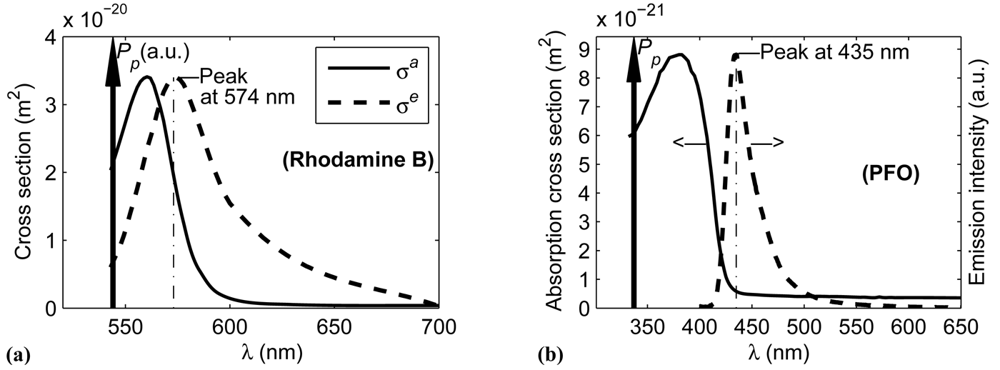
The model explained above requires the knowledge of the emission and absorption spectra of the dopant, which should be previously measured or sought in the literature on the subject. Figure 3 shows the results corresponding to POFs doped with RB and with PFO. The graphs for RB (Figure 3(a)) can be found in several papers [12], whereas those for PFO (Figure 3(b)) were determined experimentally by us [4].
As can be seen, the emission and absorption cross sections overlap significantly in the case of RB and only slightly in the case of PFO. We have analyzed the spectral shifts along the fiber length of the emitted power in both cases in order to gain some insight into the influence of the overlap. As will be shown, such changes in the spectral distribution of the emitted power can be significant, so they can serve to tune the emission of a laser or the gain of an amplifier by conveniently choosing the fiber length for a given pump power and dopant concentration.
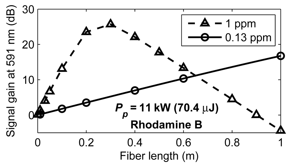
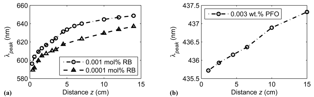
Our computational results for RB below threshold (Figure 4(a)) show a great red shift in the peak wavelength of the emitted spectrum with the two concentrations indicated in the figure, especially in the first centimeters of fiber, which is more noticeable when the concentration is higher. The same behavior is reported experimentally [18]. Even at the lower of the two concentrations, Figure 4(a) shows that λpeak changes from being less than 600 nm at z=0.5 cm to being nearly 640 nm at z = 14 cm. The concentration of 0.001 mol% of RB is about the maximum concentration achieved in [18]. The fact that the red shift is so great when the concentration of RB is high, as in both cases of (Figure 4(a)), can be explained by noting that the attenuation is also high. This increases the importance of the shape of the absorption spectrum that overlaps with the emission spectrum [18].
For the sake of comparison, we have also obtained the red shift in λpeak for the case of PFO. In this case, the curve is fairly linear and the shift is much smaller, as shown in Figure 4(b). It corresponds to a POF doped with 0.003 wt% of PFO, which is also close to the maximum that can be dissolved. However, the absorption cross section is not so high. The fact that there is a smaller part of the absorption spectrum that overlaps with the emission one explains the smaller red shift in this case. This small red shift agrees with our experimental results reported in [4].
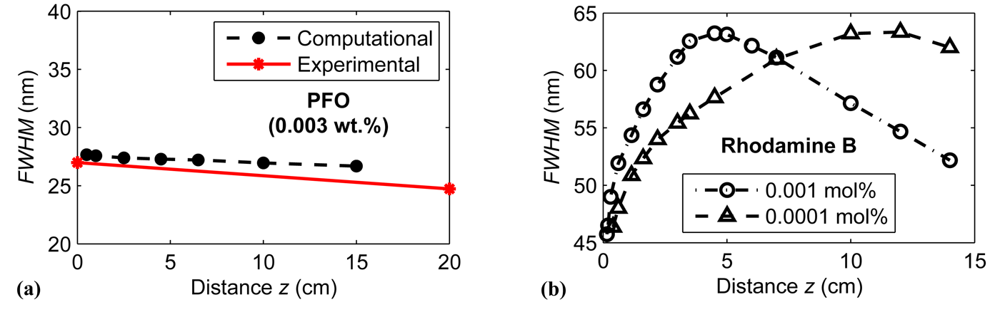
As for the change in the width of the spectrum with z below threshold, Figure 5(a) shows that the FWHM decreases slightly in a PFO-doped POF as the traveled distance increases from 0 to 15 cm, with satisfactory agreement between computational and experimental results. The dashed line was obtained by us computationally [8] and the solid one corresponds to our experimental results [4]. The changes in the spectral characteristics are much larger in the case of the RB-doped POFs already described. Even at the lower of the two concentrations of RB (0.0001 mol%), Figure 5(b) shows that the FWHM changes much more than in the case of PFO.
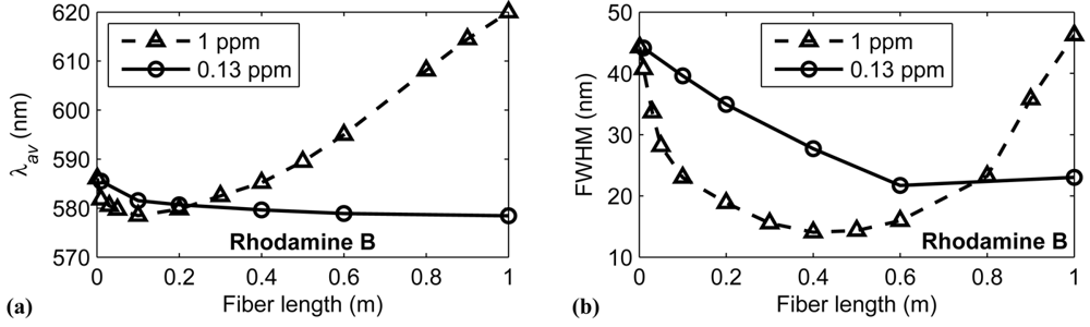
Let us now analyze what happens above threshold with the emission spectral shifts and widths in RB-doped fibers. In order to facilitate comparisons, the parameters employed in the ensuing simulations until the end of the paper are summarized in Table 2. In the figures for which a range of values of a certain parameter is used, the corresponding value of the table is not applicable.
For short fiber distances and high pump powers (above threshold), we have observed computationally a relative blue shift of the peak wavelength of P towards the maximum of the emission cross section along z. Specifically, when the pump energy is initially above threshold, there can be an initial decrease in the average wavelength of the spectrum (λav), followed by an increase, as shown in Figure 6(a) for the parameters described in Table 2 and also for a higher concentration of RB. The average wavelength is defined as . The blue shift in λav occurs especially at the beginning, when the gain in the proximity of the peak wavelength of the emission cross section is larger, which produces a relative blue shift towards the maximum of the emission cross section (Figure 6(a)). There is also an initial narrowing in the FWHM (Figure 6(b)). The explanation is similar to that of the red shift, the difference being that the influence of the emission cross section is now greater than that of the absorption one above threshold, so the effects are inverted. In other words, for a certain length of the doped fiber, the power obtained at the output at any wavelength depends on the difference between the attenuation and gain coefficients at such wavelength and on the fiber length. If the fiber length or the dopant concentration is changed, all powers at different wavelengths would also change, yielding a different output spectrum. If the pump power is increased, a blue shift towards the peak of the emission cross section is also expected even maintaining the traveled distance, as has been observed experimentally [13,25,26], since the highest gain coefficients are enhanced.
3.2. Slope Efficiency and Threshold in SI and GI POF Lasers
Firstly, by using our computational model, let us analyze the influence of NA0 (or β) on the lasing properties, such as slope efficiency and lasing threshold, in active SI and GI POFs. Some researchers define the threshold as the pump energy necessary for the full width at half maximum of the emitted intensity to drop to half the value observed when the fiber is pumped with low energy [5]. Others point out that the output energy above threshold depends linearly on the pump, define the slope efficiency as the slope of the fitting straight line, and the lasing threshold as its intersection with the horizontal axis. We have adopted the latter definitions in this section.
In order for the results to correspond to a realistic situation, we have used the same parameters as those reported in experiments [12,27], which have been summarized in Table 2. The pump energy can be easily calculated from these data by taking into account that, for a pulse that is Gaussian in time, the total energy of the pulse (E) can be related to its peak power (Pmax) through the equation E = Pmax (2π)1/2FWHM / 2.35.
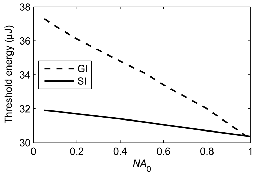
Figure 7 illustrates the influence of the fiber numerical aperture and of the pump energy on the output energy at 581 nm, for the parameters mentioned above and a core refractive index n1 = 1.492. Qualitatively, the evolution for SI and GI POFs (Figure 7(a,b) respectively) is the same. When the pump energy is low, the output is mainly due to spontaneous emissions. As a consequence, the output energy grows with a small slope. Above threshold, population inversion occurs and spontaneously emitted photons are amplified in a single pass through the fiber. At very high pump energies, incipient saturation effects are observed, which reduce the slope of the curves (see Figure 7(b)). Above threshold, the output energy reaches higher values when NA0 is higher, as expected. For higher values of NA0, there are more photons that can propagate along the fiber and interact with excited molecules, generating a higher number of stimulated emissions. In consequence there is more output energy. Considering the same NA0 for both types of fibers, it can be observed that the output energy is about four times higher in GI than in SI fibers. This means that, in the GI POF laser considered, the effect of the greater overlapping factor γ on the output energy is dominant over that of the higher average NA (or β) of the corresponding SI POF.
As can be seen in Figure 8, the pump energy needed to achieve the threshold is reduced when NA0 is higher, and the evolution is practically linear in both types of fibers. A similar behavior (i.e., a strong dependence of threshold with β) has been observed, for example, in random lasers [28], but the analysis in fibers is reported by us for the first time, as far as we know.
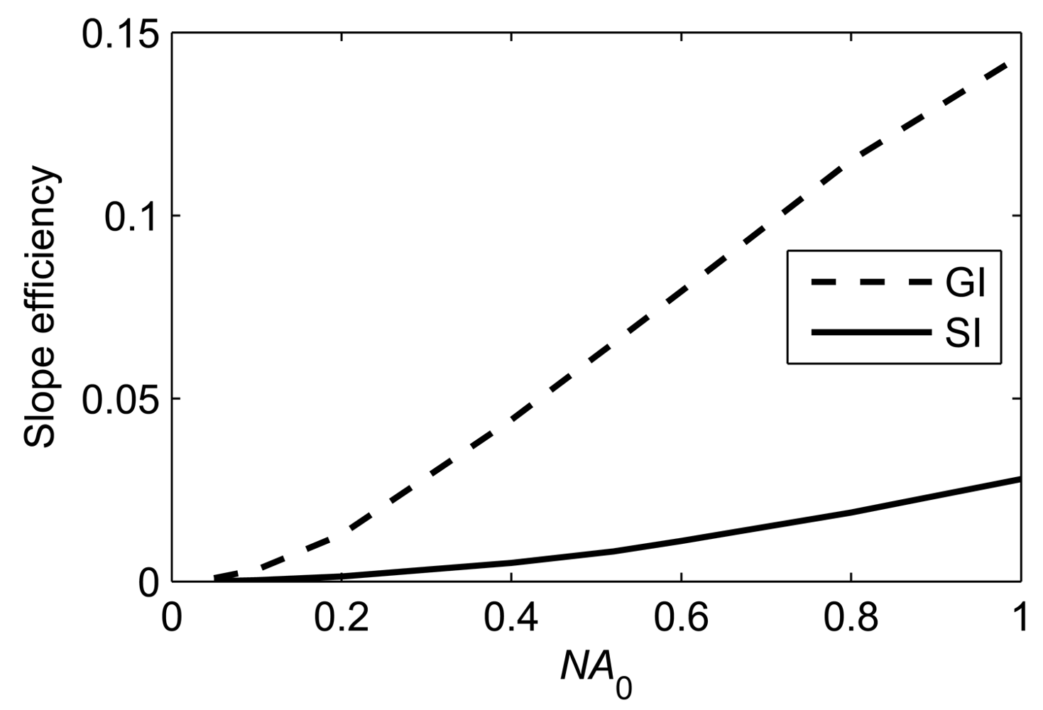
In Figure 9 we can see that the slope efficiency increases with NA0, as expected. The maximum values reached in the SI POF (solid line) are not as high as in the GI POF (dashed), showing again a dominant effect of the higher overlapping factor over the lower average value of NA in this case.
3.3. Signal Gain in SI and GI POF Amplifiers
Let us now investigate the influence of the numerical aperture on the gain of POF amplifiers. In the definition of signal gain used for optical amplifiers, the part corresponding to the power of ASE is subtracted as follows:
In this formula, Ps,in(λ) is the power of the input signal centered at wavelength λ. The numerator is the difference between the power of the amplified signal at the output of the POFA and the power of the background of ASE over the same range of wavelengths where the amplified signal appears.
We have used the same parameters as above, but in this occasion an input signal is launched as well as the pump (see Table 2). In Figure 10(a) we can see that the fraction of the output power that corresponds to the ASE increases when the numerical aperture is increased, both for SI POFs and for GI POFs with γ=1.43. This means that an increase in the axial numerical aperture NA0 tends to have a detrimental effect on the signal gain. We have also estimated, from the evolutions of the populations N1 and N2 [22], the noise figure NF, which is a measure of how much noise the ASE of the fiber amplifier adds to the signal. In this type of RB-doped amplifiers, the parameter NF can vary from about 4 dB when the fiber length is very short to about 10 dB, which has been calculated for a fiber length of 0.4 m (of still high gain) in the Figure 12 of [22]). These values are reasonable for telecommunication links. On the other hand, Figure 10(b) shows that, as expected, higher gains are achieved if γ grows in GI fibers. For any value of NA0, there can be differences in gain slightly greater than 2 dB when γ varies within the range corresponding to the three aforementioned experimental results [12,29,30]. Although γ has a noticeable influence on the signal gain, the three curves have similar slopes. Comparing the signal gains obtained in both types of fibers for the same NA0, we can note that, in the case of the GI fibers considered, the gain is significantly higher than in the SI one. This improvement in gain shows that the greater value of γ in a GI profile has more influence in this case (parameters of Table 2) than the lower average numerical aperture.
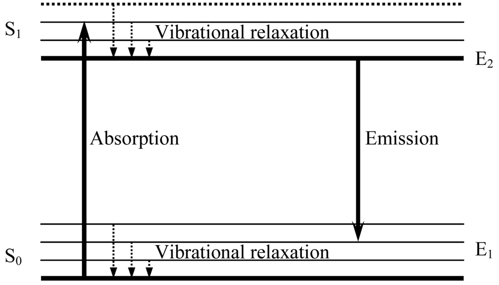
The optimum lengths (i.e., the ones yielding maximum signal gain) for several pump powers and dye concentrations) can be obtained from the maxima in Figures 11 and 12, which show the signal gain as a function of fiber length for GI and SI fibers, respectively. As can be seen in Figure 11, increasing the dye concentration of the optical fiber serves to obtain higher gains in shorter distances, and the optimum length decreases as well. For example, in GI POFAs with lengths of up to 1 m, maximum gains of nearly 30 dB can be obtained with dye concentrations of 0.13 ppm, whereas gains of nearly 40 dB are obtained with dye concentrations of 1 ppm. The corresponding experimental results [12] agree satisfactorily with the ones calculated computationally, as shown in Figure 11(a,b). Figure 12 has been calculated for the maximum pump power employed in Figure 11, and it shows that the corresponding gains at both concentrations are slightly smaller than for GI POFAs.
The highest gain in Figure 11(a) (of around 28 dB) was experimentally achieved (by the authors of [12]) with the launched pump power of 11 kW (pump energy of 70.4 μJ). Due to saturation effects, higher gains could not be achieved unless the concentration of RB was increased. When this was augmented from 0.18 ppm to 1 ppm, as shown in Figure 11(b), higher gains were obtained, the maximum one appearing for a shorter fiber length of approximately 25 cm with the same pump power of 11 kW. A practical issue that cannot be predicted by our model is that a low RB density yields a greater stability on the amplifying operation, as stated in [12]. Therefore, our results have been mainly focused on the concentration of 0.18 ppm instead of on higher ones. Besides, only pump powers up to 11 kW have been considered (5 kW in most of the Figures), since much higher ones would produce quenching and other effects, as already commented in the Section 2, which are beyond the scope of this paper.
4. Conclusions
In this work we have computationally analyzed the features of light amplification in SI and GI POFs doped with organic dyes. For this purpose, we have employed ad-hoc numerical algorithms in which the independent variables are the time, the distance traveled and the wavelength (which allows spectral analyses). The effect of the non-uniform numerical aperture in GI fibers has been calculated by introducing the average value of the fraction of spontaneously generated photons that contribute to stimulated emissions. The model also takes into account the effect of the overlap between the non-uniform dye-density and power-density radial distributions in GI POFs. From the knowledge of both distributions, we have shown how to calculate an overlapping factor γ that is introduced in the terms of the governing equations in which light powers appear multiplied by dopant concentrations.
The main results that we have obtained can be summarized as follows: (i) Firstly, we have shown the influence of the overlap between the absorption and emission cross sections of the dopant on the emission spectral shifts and widths in SI POFs. In this respect, we have seen that dyes with a strong overlap, such as rhodamine B, are suitable for tuning the spectrum of laser emission by changing the length of the doped fiber conveniently; (ii) We have also shown that an increase in the numerical aperture has a beneficial effect on the threshold power (it decreases) and on the slope efficiency (it increases) in lasers based on both SI and GI POFs doped with rhodamine B; (iii) Regarding POF amplifiers, we have shown that there is an enhancement in the signal gain when γ increases, and we have compared the results with those of SI POFs, for which γ = 1. Depending on the application, GI POF amplifiers or SI POF amplifiers can be employed, with some advantage in signal gain in GI POF amplifiers over SI ones. The optimum signal wavelength and pump power as functions of the fiber length, the fiber numerical aperture and the radial distribution of the dopant have also been analyzed, for both SI and GI POFs. In both GI and SI POFAs, the signal gain does not significantly change with variations in the numerical aperture.
These analyses can be useful to designing amplifiers and lasers based on polymer optical fibers.


| Step Index | Graded Index | |||
|---|---|---|---|---|
| Equation | Value | Equation | Value | |
| β | 0.029 | 0.028 | ||
| γ | – | 1 | 1.43 | |
| Parameter | Notation | Value |
|---|---|---|
| Signal power (if any) | Ps | 1 W |
| Signal wavelength | λs | 591 nm |
| Signal full width at half maximum | FWHM | 3.5 ns |
| Pump power | Pp | 5 kW (11 kW for Figures 6 and 12) |
| Pump wavelength | λp | 532 nm |
| Pump full width at half maximum | FWHM | 6 ns |
| Signal attenuation | α(λs) = αs | 8.50 dB/m |
| Pump attenuation | α(λp) = αp | 8.13 dB/m |
| Fiber length | L | 1 m |
| Core radius | a0 | 0.25 mm |
| Absorption cross section at λp | σa(λp) | 2.2×10⁻²⁰ m2 |
| Emission cross section at λs | σe(λs) | 2.3×10⁻²⁰ m2 |
| Spontaneous lifetime of RB | τ | 2.85 ns |
| Dopant concentration | – | 0.13 ppm |
Acknowledgments
This work was supported by the Ministerio de Ciencia e Innovación under projects TEC2009-14718-C03-01 and COBOR, by the Gobierno Vasco/Eusko Jaurlaritza under projects GIC07/156-IT-343-07, AIRHEM, S-PR10UN04, and S-PE10CA01, and by the Diputación Foral de Bizkaia/Bizkaiko Foru Aldundia under project 06-12-TK-2010-0022. The research leading to these results has also received funding from the European Commission's Seventh Framework Programme (FP7) under grant agreement no. 212912 (AISHA II). I. Ayesta has a research fellowship from Vicerrectorado de Euskara y Plurilingüismo, Universidad del País Vasco/Euskal Herriko Unibertsitatea (UPV/EHU), while working on his PhD.
Appendix: Calculation of the Parameters β and γ
In the case of a GI fiber, an average value of β should be calculated. This is accomplished as follows. The fraction of guided directions βr(r) as a function of the radial distance r is
We will maintain n1 constant in all cases (the same core) and we will consider the influence of the refractive index of the cladding. For the typical values n1 = 1.492 and n2 = 1.402, we obtain that β is 0.028, so this has been the average value employed for most of our simulations. The minimum possible average value β is 0, which would happen if n1 = n2, although this is only a theoretical limit, since it would imply a flat refractive-index profile. The maximum one is approximately 0.15, which happens when n2 = 1, i.e., in an uncladded POF.
Regarding the overlapping factor γ, according to [22] it can be defined as:
The way we normalize both distributions is as follows. As stated before, if both θ(r) and ψ(r) were constant (θ and ψ0 respectively), then γ would be 1, so:
Since θ0 is the average dopant concentration:
And similarly for the light power:
Usually, non-normalized graphs of dopant and light power distributions are reported [12,29,30]. We call them θnn(r) and ψnn(r) respectively. Their normalized counterparts are proportional to them:
From Equations (A5) and (A6), the values of k1 and k2 in (A7) are:
Finally, from Equation (A3), and using Equations (A4), (A7) and (A8):
The data needed to evaluate γ numerically using Equation (A9) is available from experimental results. The value that we have obtained using [12] is γ = 1.43. Although γ could take any value from 0 to ∞, realistic values are not very different from 1.4. For example, γ = 1.53 is obtained from [29] and γ = 1.36 from [30].
References
- Zubia, J.; Arrue, J. Plastic optical fibers: An introduction to their technological processes and applications. Fiber Technol. 2001, 7, 101–140. [Google Scholar]
- Maier, G.V.; Kopylova, T.N.; Svetlichnyi, V.A.; Podgaetskii, V.M.; Dolotov, S.M.; Ponomareva, O.V.; Monich, A.E. Active polymer fibres doped with organic dyes: Generation and amplification of coherent radiation. Quantum Electron. 2007, 37, 53–59. [Google Scholar]
- Sheeba, M.; Thomas, K.J.; Rajesh, M.; Nampoori, V.P.N.; Vallabhan, C.P.G.; Radhakrishnan, P. Multimode laser emission from dye doped polymer optical fiber emission from dye doped polymer optical fiber. Appl. Opt. 2007, 46, 8089–8094. [Google Scholar]
- Illarramendi, M.A.; Zubia, J.; Bazzana, L.; Durana, G.; Aldabaldetreku, G.; Sarasua, J.R. Spectroscopic characterization of plastic optical fibers doped with fluorene oligomers. J. Lightwave Technol. 2009, 27, 3220–3226. [Google Scholar]
- Clark, J.; Bazzana, L.; Bradley, D.D.C.; Cabanillas-Gonzalez, J.; Lanzani, G.; Lidzey, D.G.; Morgado, J.; Nocivelli, A.; Tsoi, W.C.; Virgili, T.; Xia, R. Blue polymer optical fiber amplifiers based on conjugated fluorine oligomers. J. Nanophoton. 2008, 2, 521–531. [Google Scholar]
- Liang, H.; Zheng, Z.; Li, Z.; Xu, j.; Chen, B.; Zhao, H.; Zhang, Q. Fabrication and amplification of rhodamine B-doped step-index polymer optical fiber. J. Appl. Polym. Sci. 2004, 93, 681–685. [Google Scholar]
- Tagaya, A.; Koike, Y.; Kinoshita, T.; Nihei, E.; Yamamoto, T.; Sasaki, K. Polymer optical fiber amplifier. Appl. Phys. Lett. 1993, 53, 883–884. [Google Scholar]
- Arrue, J.; Jimenez, F.; Illarramendi, M.A.; Zubia, J.; Ayesta, I.; Bikandi, I.; Berganza, A. Computational analysis of the power spectral shifts and widths along dye-doped polymer optical fibers. IEE Photonics J. 2010, 2, 521–531. [Google Scholar]
- Ishigure, T.; Kano, M.; Koike, Y. Which is a more serious factor to the bandwidth of GI POF: Differential mode attenuation or mode coupling? J. Lightwave Technol. 2000, 18, 959–965. [Google Scholar]
- Samuel, I.D.W.; Turnbull, G.A. Organic semiconductor lasers. Chem. Rev. 2007, 107, 1272–1295. [Google Scholar]
- Kobayashi, T.; Kuriki, K.; Imai, N.; Tamura, T.; Sasaki, K.; Koike, Y. High-power polymer optical fiber lasers and amplifiers. Proc. SPIE 1999, 3623, 206–214. [Google Scholar]
- Tagaya, A.; Teramoto, S.; Yamamoto, T.; Fujii, K.; Nihei, E.; Koike, Y.; Sasaki, K. Theoretical and experimental investigation of rhodamine B-doped polymer optical fiber amplifiers. IEEE J. Quant. Electron. 1995, 31, 2215–2220. [Google Scholar]
- Rajesh, M.; Sheeba, M.; Geetha, K.; Vallaban, C.P.G.; Radhakrishnan, P.; Nampoori, V.P.N. Fabrication and characterization of dye-doped polymer optical fiber as a light amplifier. Appl. Opt. 2007, 46, 106–112. [Google Scholar]
- Peng, G.D.; Xiong, Z.; Chu, P.L. Fluorescence decay and recovery in organic dye-doped polymer optical fibers. J. Lightwave Technol. 1998, 16, 2365–2372. [Google Scholar]
- Tagaya, A.; Koike, Y.; Nihei, E.; Teramoto, S.; Fujii, K.; Yamamoto, T.; Sasaki, K. Basic performance of an organic dye-doped polymer optical fiber amplifier. Appl. Opt. 1995, 34, 988–992. [Google Scholar]
- Charas, A.; Mendonça, A.L.; Clark, J.; Cabanillas-Gonzalez, J.; Bazzana, L.; Nocivelli, A.; Lanzani, G.; Morgado, J. Gain and ultrafast optical switching in PMMA optical fibers and films doped with luminescent conjugated polymers and oligomers. Front. Optoelectron. China 2010, 3, 45–53. [Google Scholar]
- Tagaya, A.; Teramoto, S.; Nihei, E.; Sasaki, K.; Koike, Y. High-power and high-gain organic dye-doped polymer optical fiber amplifiers: Novel techniques for preparation and spectral investigation. Appl. Opt. 1997, 36, 572–578. [Google Scholar]
- De la Rosa-Cruz, E.; Dirk, C.W.; Rodríguez, A.; Castaño, V.M. Characterization of fluorescence induced by side illumination of rhodamine B doped plastic optical fibers. Fiber Integr. Opt. 2001, 20, 457–464. [Google Scholar]
- Samuel, I.D.W.; Namdas, B.; Turnbull, G.A. How to recognize lasing. Nat. Photon. 2009, 10, 546–549. [Google Scholar]
- Amarasinghe, D.; Ruseckas, A.; Turnbull, G.A.; Samuel, I.D.W. Organic semiconductor optical amplifiers. Proc. IEEE 2009, 97, 1637–1650. [Google Scholar]
- Speiser, S.; Shakkour, N. Photoquenching parameters for commonly used laser dyes. Appl. Phys. B 1985, 38, 191–197. [Google Scholar]
- Karimi, M.; Granpayeh, N.; Farshi, M.K.M. Analysis and design of a dye-doped polymer optical amplifier. Appl. Phys. B 2004, 78, 387–396. [Google Scholar]
- Xia, R.; Heliotis, G.; Hou, Y.; Braddley, D.D.C. Fluorene-based conjugated polymer optical gain media. Organ. Electron. 2003, 4, 165–177. [Google Scholar]
- Kuriain, A.; George, N.A.; Paul, B.; Nampoori, V.P.N.; Vallabhan, C.P.G. Studies on fluorescence efficiency and photodegradation of rhodamine 6G doped PMMA using a dual beam thermal lens technique. Laser Chem. 2002, 20, 99–110. [Google Scholar]
- Wang, H.Z.; Zhao, F.L.; He, Y.J.; Zheng, X.G.; Huang, X.G.; Wu, M.M. Low-threshold lasing of a rhodamine dye solution embedded with nanoparticle fractal aggregates. Opt. Lett. 1998, 23, 777–779. [Google Scholar]
- Lam, S.Y.; Damzen, M.J. Characterisation of solid-state dyes and their use as tunable laser amplifiers. Appl. Phys. B 2004, 77, 577–584. [Google Scholar]
- Tagaya, A.; Kobayashi, T.; Nakatsuka, S.; Nihei, E.; Sasaki, K.; Koike, Y. High gain and high power organic dye-doped polymer optical fiber amplifiers: Absorption and emission cross sections and gain characteristics. Jpn. J. Appl. Phys. 1997, 36, 2705–2708. [Google Scholar]
- Van Soest, G.; Lagendijk, A. β factor in a random laser. Phys. Rev. E 2003, 65, 047601. [Google Scholar]
- Kuriki, K.; Kobayashi, T.; Imai, N.; Tamura, T.; Koike, Y.; Okamoto, Y. Organic dye-doped polymer optical fiber laser. Polym. Adv. Technol. 2000, 11, 612–616. [Google Scholar]
- Sasaki, K.; Koike, Y. Polymer Optical Fibre Amplifier. U.S. Patent 5,450,232,12, 12 September 1995. [Google Scholar]
© 2011 by the authors; licensee MDPI, Basel, Switzerland. This article is an open access article distributed under the terms and conditions of the Creative Commons Attribution license (http://creativecommons.org/licenses/by/3.0/).
Share and Cite
Arrue, J.; Jiménez, F.; Ayesta, I.; Illarramendi, M.A.; Zubia, J. Polymer-Optical-Fiber Lasers and Amplifiers Doped with Organic Dyes. Polymers 2011, 3, 1162-1180. https://doi.org/10.3390/polym3031162
Arrue J, Jiménez F, Ayesta I, Illarramendi MA, Zubia J. Polymer-Optical-Fiber Lasers and Amplifiers Doped with Organic Dyes. Polymers. 2011; 3(3):1162-1180. https://doi.org/10.3390/polym3031162
Chicago/Turabian StyleArrue, Jon, Felipe Jiménez, Igor Ayesta, M. Asunción Illarramendi, and Joseba Zubia. 2011. "Polymer-Optical-Fiber Lasers and Amplifiers Doped with Organic Dyes" Polymers 3, no. 3: 1162-1180. https://doi.org/10.3390/polym3031162