Optimal Focusing and Scaling Law for Uniform Photo-Polymerization in a Thick Medium Using a Focused UV Laser

Abstract

We present a modeling study of photoinitiated polymerization in a thick polymer-absorbing medium using a focused UV laser. Transient profiles of the initiator concentration at various focusing conditions are analyzed to define the polymerization boundary. Furthermore, we demonstrate the optimal focusing conditions that yield more uniform polymerization over a larger volume than the collimated or non-optimal cases. Too much focusing with the focal length f < f* (an optimal focal length) yields a fast process; however, it provides a smaller polymerization volume at a given time than in the optimal focusing case. Finally, a scaling law is derived and shows that f* is inverse proportional to the product of the extinction coefficient and the initiator initial concentration. The scaling law provides useful guidance for the prediction of optimal conditions for photoinitiated polymerization under a focused UV laser irradiation. The focusing technique also provides a novel and unique means for obtaining uniform photo-polymerization within a limited irradiation time.

1. Introduction

UV-photoinitiated polymerization provides advantages over thermal-initiated polymerization, including fast and controllable reaction rates without a need for high temperatures or specific pH conditions [1,2,3,4]. Furthermore, it offers control over the process, which is sensitive to wavelength. The maximum rate can be achieved by optimizing polymer parameters, such as concentration and absorptivity.

The kinetics of photoinitiated polymerization have been studied by many researchers analytically, numerically, and experimentally [2,3,4,5,6,7,8,9,10,11,12]. In general, the laser may still be absorbed by the photolysis product; therefore, the kinetics of photoinitiated polymerization, especially in thick polymer systems, become difficult to solve analytically, and only numerical results have been reported in previous work [9,10,11,12]. Commercial type-I photoinitiators that produce two radicals following visible photon absorption have limited water solubility and high cell toxicity [1]. A UV laser at 365 nm was used for improved polymerization kinetics at lower initiator concentrations [4]. Review of various kinetic conditions and different photosensitizers are available [13,14].

We have recently developed semi-analytic modeling for photo-polymerization in a thick polymer (up to 10 mm) [15] and for corneal cross linking [16] under a collimated UV laser. We have optimized the initiator concentration, C(z,t), to achieve a maximum value of the photoinitiation rate, R(z,t), which has a profile defined by the path of light propagation inside the polymer (z) and the irradiation time (t). For small t, R(z,t) follows the same trend as the light intensity I(z,t) and increases with z. For larger t, a reversal is seen in the trend of R(z,t) due to the competing processes between I(z,t) and C(z,t), where an increase of C(z,t) in z dominates, and therefore, the R(z,t) profile shows a peak value at certain z values. This intrinsic feature causes a non-uniform z-distribution of the photo-polymerization rate. The photo-polymerization is always faster at the entrance and slower at the exit of the absorbing medium. Therefore, thick absorbing media (>1.0 cm) cannot be completely photopolymerized, especially the bottom portion.

The above-described drawback exists for all photoinitiated systems that rely on illumination by a collimated laser beam, whose intensity decreases exponentially as a function of z inside the absorbing medium. To overcome the drawback of a collimated laser system and achieve a more uniform photo-polymerization throughout the whole medium, this study presents a focused laser system. We will first introduce a focusing function to compensate for the exponential decay in laser intensity inside the absorbing medium. The polymerization equation is analyzed for optimal conditions and numerically evaluated. The polymerization process is defined by the time evolution of polymerization boundaries.

To the best of our knowledge, this study provides the first presentation of a scaling law for optimal focusing, governed by the extinction coefficient and the initial concentration of the initiator. The focusing technique also provides a novel and unique means for uniform photo-polymerization (within a limited time of irradiation), which cannot be achieved by any other means.

2. Method and Theory

2.1. The Focused Laser

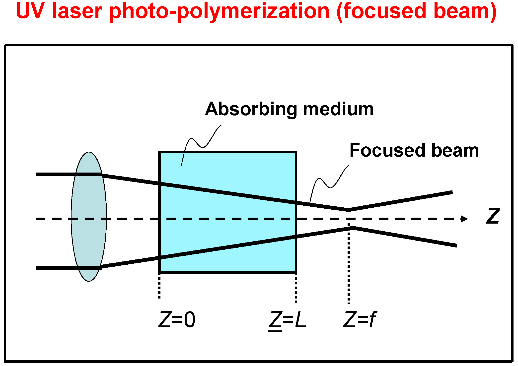
As shown in Figure 1, a UV laser is focused while propagating along the z-direction, which represents the thickness of the absorbing medium having the UV photoinitiator. The initial (at t = 0) laser intensity (or fluence) of a focused beam may be expressed in analytic form as:

I(z,t = 0) = I₀F(z)

(1)

where F(z) is a focusing function:

(2a)

(2b)

In Equation (1), I₀ = I(z−0,t) is the laser intensity at the entrance plane (z = 0) of the medium and w is the ratio between the beam spot size at z = 0 and the spot size at the focal point (z = f). Here, we have defined f as the effective focal length including the beam refraction due to the absorbing medium. The focal length of the lens (in air) is shorter than this effective focal length by a factor of the polymer medium refractive index, about 1.33.

Figure 1. Schematic of a focused UV laser propagating through an absorbing medium having thickness L.

Figure 1. Schematic of a focused UV laser propagating through an absorbing medium having thickness L.

2.2. The Kinetic Equations

For a thick polymerization system illuminated by a UV laser, the laser intensity, the photoinitiator and the photolysis product concentration, should be governed by a three-dimensional diffusion equation that can only be solved numerically. For a comprehensive analysis with an emphasis on the focusing features, we will ignore the diffusion effects such that the initiator profile may be described by a set of first-order differential equations.

The molar concentration of the photoinitiator C(z,t) and the focused UV laser intensity I(z,t) can be described by a one-dimensional kinetic model [9,10,11,12], which is revised in this study to include the focusing effect as follows:

(3a)

and:

(3b)

where F(z) is the focusing function defined by Equation (2); C₀ is the initial value, C₀ = C(z,t = 0); a = 83.6λφε₁, with φ being the quantum yield and λ being the laser wavelength; and ε₁ and ε₂ are the molar extinction coefficient of the initiator and the photolysis product, respectively. In our calculations, the following units are used: C(z,t) in mM, I(z,t) in (mW/cm²), λ in cm, z in cm, t in seconds, and ε_j in (mM·cm) ⁻¹. As with the conditions of references 9–12, we have ignored inhibition or self-focusing effects, which might be important in high light intensity case, but not in our low intensity case, 10–50 (mW/cm²). Review of various kinetic conditions and different photosensitizers may be found in [13,14].

The coupled differential equations were solved, by finite element method, with the initial boundary conditions C(z,0) = C₀ and I(0,t) = I₀. According to Equation (3), we can also obtain the additional conditions C(0,t) = C₀ exp(−aI₀t) and I(z,0) = I₀F(z)exp(−2.303ε₁C₀z). For the simplified case with ε₂ = 0 and a collimated beam with F(z) = 1, the analytic solutions for a photoinitiated polymerization process have been derived by previous researchers [5,6,7,8]. For the general case with ε₂ ≠ 0, in which the photolysis product may still partially absorb the UV laser, the coupled differential Equations (3a) and (3b) become very difficult to solve analytically, and therefore, only numerical results (limited to the collimated case) have been reported thus far [9,10,11,12,15,16].

2.3. Analytic Formulas

From our numerical results, shown later, the initiator concentration has a slowly varying spatial distribution, and thus, Equation (3) can be approximated to the first order as:

(4a)

where C₍₀₎(z,t) is the zero-th order solution of Equation (3a) and is given by:

(4b)

where b = 2.303(ε₁ − ε₂) and h = 2.303ε₂. Substituting Equation (4a) to Equation(3a), we may easily find the integral expression for the first order solutions of the initiator concentration as follows:

(5)

The above equations provide an explicit formula for C(z,t) as a function of z, t, C₀, and I₀. Equations (4) and (5) show that the initiator concentration is a deceasing function of time (t); however, the laser intensity increases with time due to photobleaching of C(z,t). Equation (4a) shows that I(z,t) is an exponential decreasing function of z due to the term bC(z,t), which is proportional to (ε₁C₀). Therefore, a higher concentration, shorter focusing, or a smaller f in F(z) is needed for larger (ε₁C₀). These two factors that compete in z provide us with the important realization that there is an optimal focus such that a uniform profile (up to a certain medium thickness) of C(z,t) is achievable. Later, our numerical calculations will demonstrate the above analysis.

2.4. Photoinitiation Rate

If two active centers are produced upon defragmentation of the initiator, the local photoinitiation rate for the production of free radicals, R(z,t), is represented by [5]:

R(z,t) = 2ε₁ϕI(z,t)C(z,t)

(6)

From the first order approximation shown by Equations (4) and (5), we readily see that the photoinitiation rate is proportional to ε₁C₀, and the laser intensity is a competing, deceasing function of ε₁C₀. Therefore, an optimal value of ε₁C₀ can be expected for a maximum photoinitiation rate derived from the balance between these two competing factors. The optimal condition will be shown in next section.

2.5. The Optimization

From Equation (5), for a given optimal focal length (f*), there will be a range of z values such that the profiles of C(z,t) achieve a nearly flat top. This feature defines uniform photo-polymerization in a thick medium and cannot be achieved by a collimated beam. Due to the complexity of the z-dependence of C(z,t) and I(z,t), the exact optimization condition can only be numerically obtained. However, the qualitative trend is that a long focal length will provide a large range (z) of a flat profile, and the optimal focal length (f*) shall be governed by a scaling law f* ∞ 1/(ε₁C₀*). This scaling prediction, based on our analytic formulas, will be quantitatively demonstrated later with numerical simulations.

3. Numerical Results and Discussions

Equation (3) will be solved using the finite element method. First, we will study the case of a collimated beam, where F(z) = 1 in Equation (3). The roles of ε₁ and C₀ on the transient profiles of C(z,t) and R(z,t) will be analyzed. We will then demonstrate the optimal focal length for achieving a uniform photoinitiation, which is a special feature that cannot be achieved by a collimated beam.

3.1. Collimated Beam

For a collimated beam, F(z) = 1 in Equation (3), the profiles of the normalized concentration C(z,t) have been solved using parameters referring to the experiment work of Fairbanks et al. [4]: λ = 3.65 × 10⁻⁵ cm, ϕ = 1.0 and ε₂ = 0.075 (mM·cm)⁻¹. However, we have used a higher laser intensity, I₀ =20 mW, to shorten the time needed for the polymerization process.

The initiator concentration, C(z,t), is depleted by the UV laser as time evolves. However, at a given time, it is an increasing function of the thickness (z) due to the reduced laser intensity as z increases. This feature may also be realized mathematically by the approximate solution of the initiator concentration , where A(z) = exp[−hC₀z] is a decreasing functioning of z such that C(z,t) is an increasing function of z at a given time.

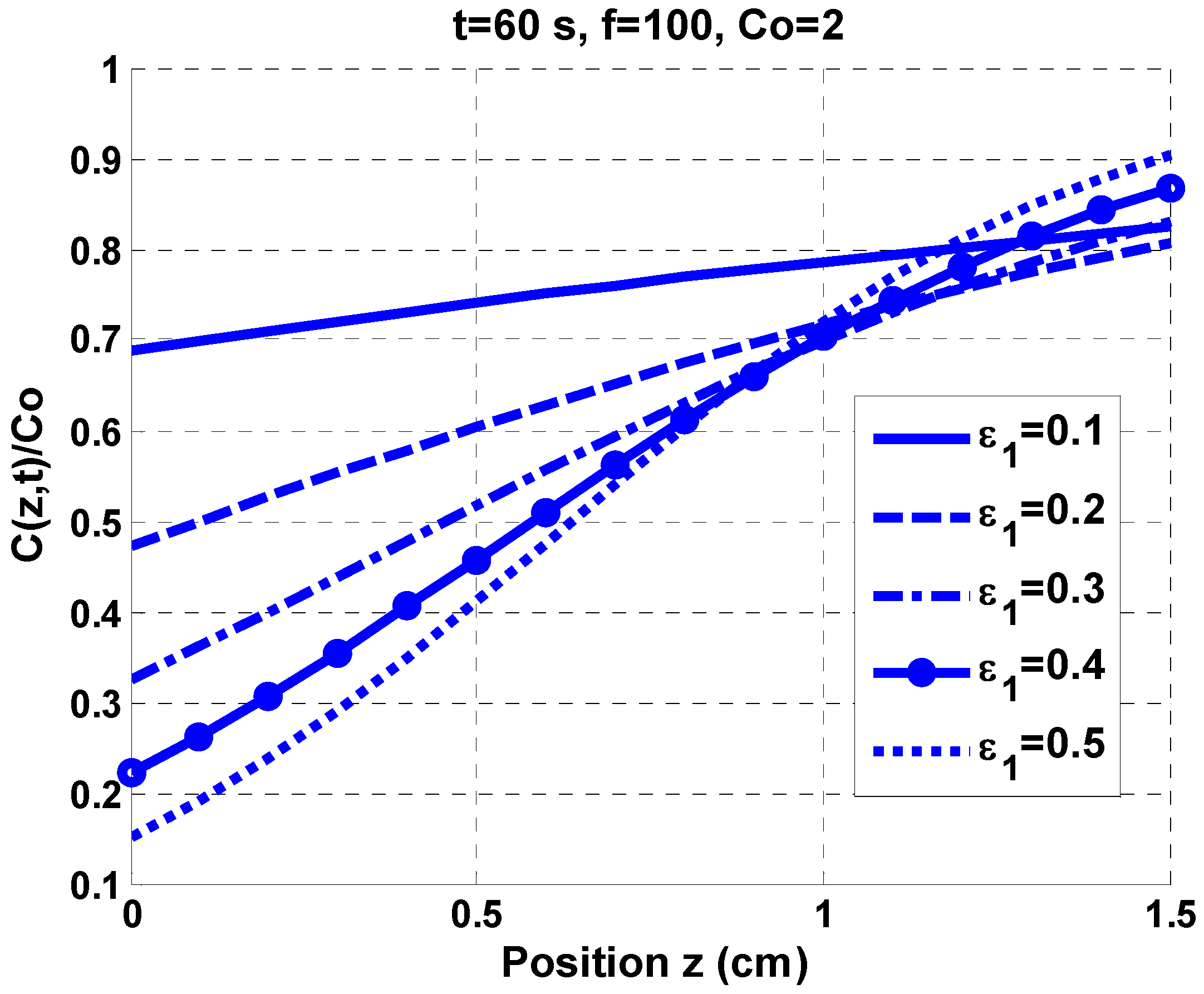
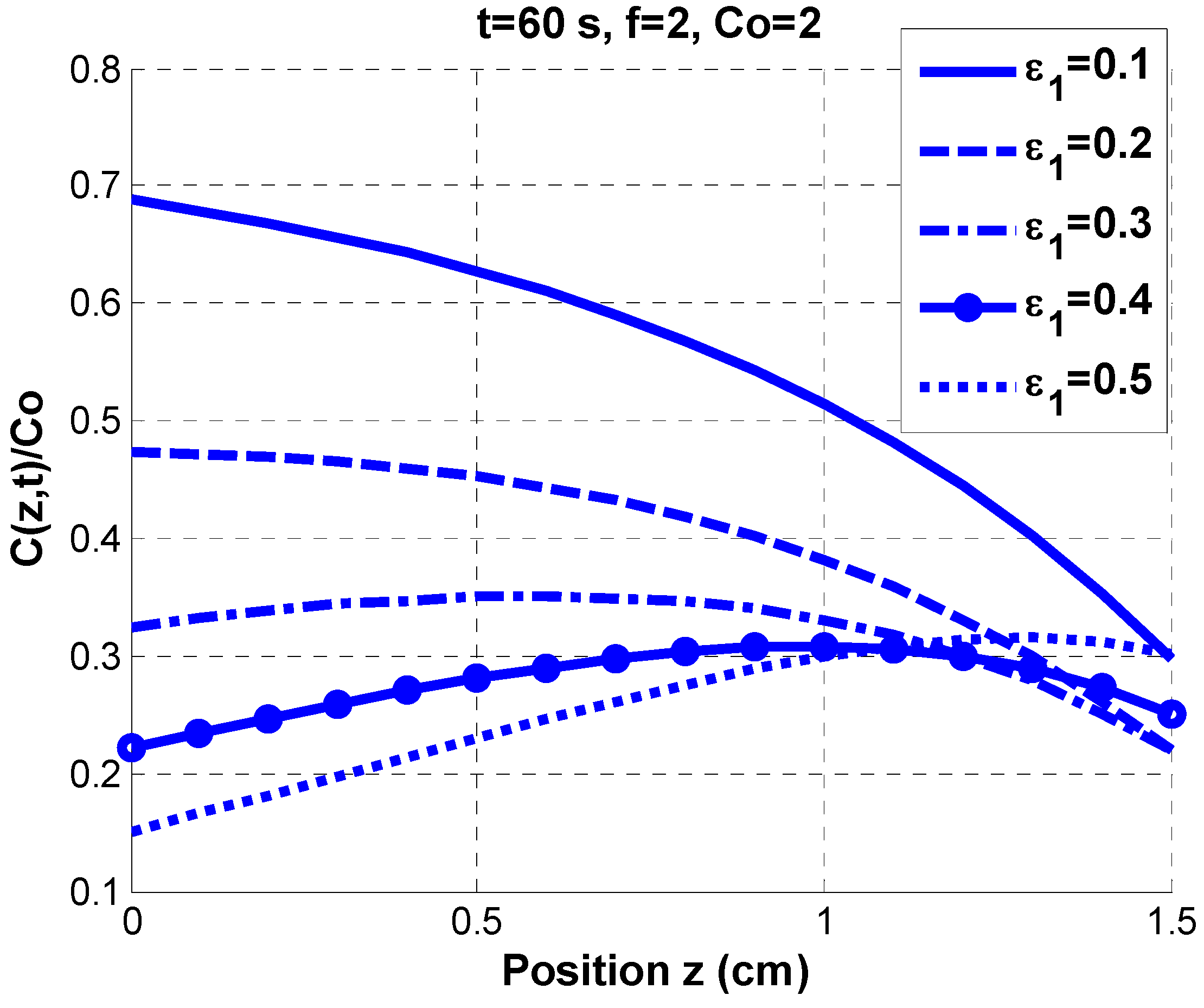
Figure 2 shows the role of the extinction coefficient of the initiator (ε₁) on the profiles of the normalized C(z,t) for a fixed initial value C₀ = 2.0 mM at t = 60 s. It shows a higher slope (or increasing rate) of the C(z,t) profiles for larger ε₁, which defines the coupling strength between the laser and the absorbing medium. In other words, larger coupling provides faster depletion of the initiator concentration, in which the depletion boundary always starts from the entrance plane (z = 0) and gradually moves to the output plane (z = L) of the medium. This feature, occurring in all systems irradiated by a collimated beam, limits the polymerization to a thin layer of 0.1 to 0.3 cm, and partial polymerization is usually found in a thick medium having L > 0.5 cm. The non-uniform distribution (in z) of C(z,t) produced by a collimated beam may be significantly improved by using a focused beam. We should note that the completion of the polymerization process at a given time may be defined by the amount of remaining C(z,t). Therefore, a higher value of C(z,t)means a lower degree of polymerization.

Figure 2. Profiles of normalized initiator concentration C(z,t)/C₀ versus polymer thickness (z) for various extinction coefficients of the initiator, ε₁ = 0.1 to 0.5 (mM·cm)^–1, at an irradiation time t = 60 s using a collimated beam.

Figure 2. Profiles of normalized initiator concentration C(z,t)/C₀ versus polymer thickness (z) for various extinction coefficients of the initiator, ε₁ = 0.1 to 0.5 (mM·cm)^–1, at an irradiation time t = 60 s using a collimated beam.

3.2. Focused Beam

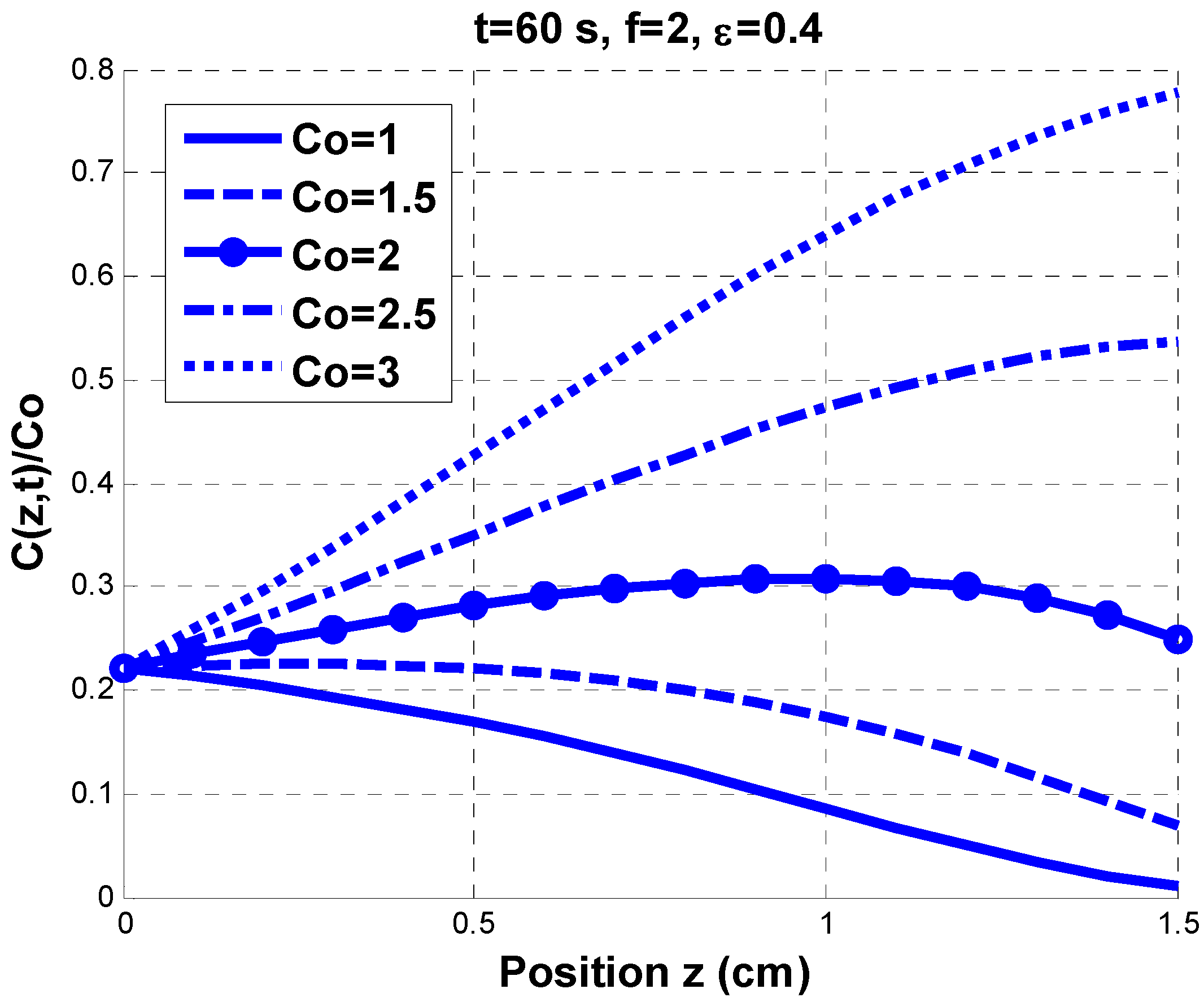
In Equation (2), the focusing function, F(z), is expressed in terms of w and f, in which the value of w depends on the beam divergent angle and beam quality of the focused laser. In this study, we will assume w = 0.2 for a typical diode laser as the UV light source. If an light emitting diode (LED) is used as the light source, w will be larger (0.4 to 0.6). Figure 3 shows the calculated profiles (at t = 60 s) of the normalized concentration C(z,t)/C₀ for a fixed ε₁ = 0.4 (mM·cm)⁻¹ and various initial values of C₀.

In Figure 3, a focused UV laser with a focal length f = 2.0 cm is used to suppress the increasing profiles of C(z,t) such that a more uniform distribution (along the medium thickness direction z) may be achieved. It can be seen that f = 2.0 cm is an optimized focal length for an almost uniform C(z,t) along the z-direction for the entire medium thickness, L = 1.5 cm. However, this focal length is only applicable to the profile of C₀ = 2.0 mM. It is too focused for smaller C₀ < 2.0 and not focused enough for larger C₀ > 2.5. In other words, a shorter focal length is needed for a larger C₀.

The data from Figure 3 and Figure 4 indicate that the optimal focal length (f*) should be governed by the product of ε₁ and C₀. This feature led us to search for a scaling law of f* defined by (ε₁C₀) in the next section.

Figure 3. Profiles of normalized initiator concentration C(z,t)/C₀ for a focused beam (with focal length f = 2.0 cm) at t = 60 s and a given extinction coefficient of the initiator, ε₁ = 0.4 (mM·cm)⁻¹, but for various initial concentrations C₀ = 1.0 to 3.0 mM.

Figure 3. Profiles of normalized initiator concentration C(z,t)/C₀ for a focused beam (with focal length f = 2.0 cm) at t = 60 s and a given extinction coefficient of the initiator, ε₁ = 0.4 (mM·cm)⁻¹, but for various initial concentrations C₀ = 1.0 to 3.0 mM.

Figure 4. As Figure 3, but for a fixed C₀ = 20 mM and various ε₁ = 0.1 to 0.4 (mM·cm)⁻¹.

Figure 4. As Figure 3, but for a fixed C₀ = 20 mM and various ε₁ = 0.1 to 0.4 (mM·cm)⁻¹.

3.3. The Scaling Law

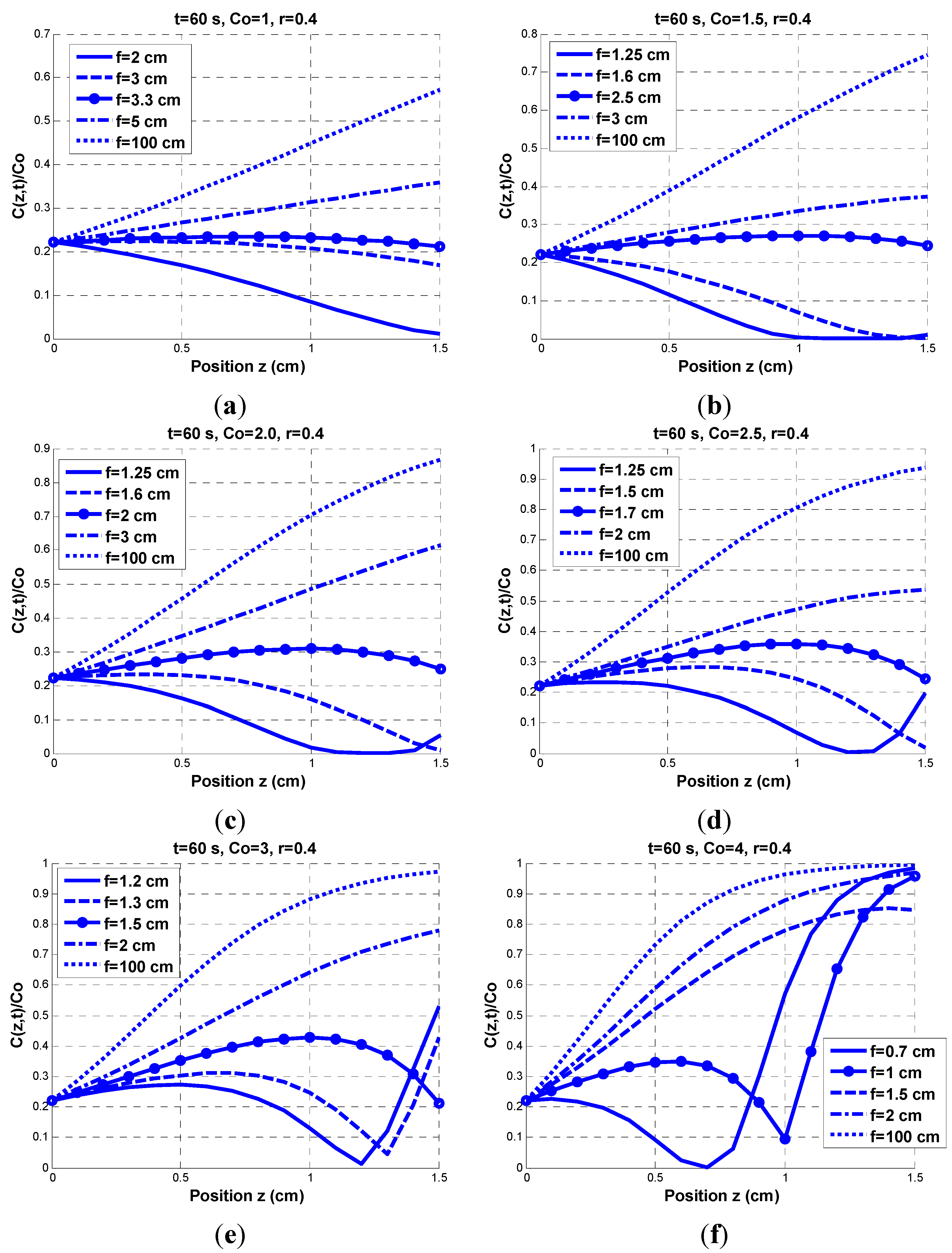
As shown by Figure 5a–f, the profiles of C(z,t) are calculated for various degrees of focusing, for a given ε₁ = 0.4 (mM·cm)⁻¹, t = 60 s and various C₀ between 1.0 and 4.0 mM. The optimal focal lengths (f*) are defined as occurring when the C(z,t = 60 s) profiles reach their most uniform distributions along the z direction.

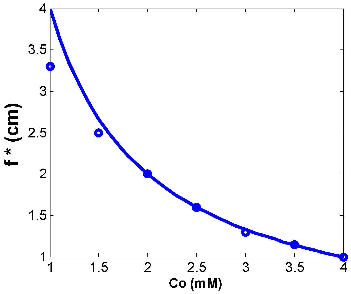
We obtained f* = (3.3, 2.5, 2.0, 1.6, 1.3, 1.15, 1.0) cm for C₀ = (1.0, 1.5, 2.0, 2.5, 3.0, 3.5, 4.0) mM, with ε₁ =0.4 (mM·cm)⁻¹ and t = 60 s. These calculated f* values can be fit to a scaling law equation given by f* = 1.6/(ε₁C₀). This scaling law is based on the numerical calculations and was also discussed based on our earlier analytic formulas, Equations (4) and (5). Figure 6 shows the scaling law curve and the calculated f*, where a larger ε₁C₀ requires a tighter focusing, or smaller f*, to achieve a uniform profile of C(z,t), which corresponds to a uniform polymerization process along the medium thickness (z). More details will be discussed in the next section.

Figure 5. Profiles (A to F) of normalized initiator concentration C(z,t)/C₀ at t = 60 s for a focused beam having various focal lengths and a given extinction coefficient of the initiator 0.4 (mM·cm)⁻¹. The initial concentration, C₀, was varied between 1.0 and 4.0 mM (for Figure 5a–f). The profiles produced by the optimal focal lengths are shown by dotted curves. (a) C₀ = 1.0; (b) C₀ = 1.5; (c) C₀ = 2.0; (d) C₀ = 2.5; (e) C₀ = 3.0; (f) C₀ = 4.0 (mM).

Figure 5. Profiles (A to F) of normalized initiator concentration C(z,t)/C₀ at t = 60 s for a focused beam having various focal lengths and a given extinction coefficient of the initiator 0.4 (mM·cm)⁻¹. The initial concentration, C₀, was varied between 1.0 and 4.0 mM (for Figure 5a–f). The profiles produced by the optimal focal lengths are shown by dotted curves. (a) C₀ = 1.0; (b) C₀ = 1.5; (c) C₀ = 2.0; (d) C₀ = 2.5; (e) C₀ = 3.0; (f) C₀ = 4.0 (mM).

Figure 6. Curve based on a scaling law. In addition, shown as dots are the data based on the calculated f* (referring to Figure 5a–f).

Figure 6. Curve based on a scaling law. In addition, shown as dots are the data based on the calculated f* (referring to Figure 5a–f).

3.4. The Kinetics of Polymerization

We should note that the completion of the polymerization process at a given time may be defined by the amount of remaining C(z,t). Therefore, higher values of C(z,t) correspond to a lower degree of polymerization. We may define the boundary of the polymerization as when the initiator concentration is depleted to 30% of its initial value after a certain time (t) of laser irradiation, that is, when C(z,t)/C₀ > 0.3. The uncompleted polymerization is shown by the area with C(z,t)/C₀ > 0.3.

We first show the collimated case. The time evolution of the polymerization boundary may be seen by the crossing positions of the horizontal red-line C(z,60)/C₀ = 0.3 and the transient C(z,t) profiles. As shown by Figure 7, the polymerization process starts from the surface (z = 0, at approximately t = 5 s) and moves to approximately z = 0.5 cm at t = 90 s. Figure 7 demonstrates the drawback of a collimated beam because it limits the polymerization to a thin layer (approximately 0.5 cm). This limitation may be removed by focusing the beam, as shown in Figure 8 and Figure 9.

Figure 7. Profiles of the initiator concentration under collimated laser polymerization, where the time evolution of the polymerization boundary is defined by the crossing positions of the horizontal red-line C(z,60)/C₀ = 0.3. Curves 1 to 9 are profiles at t = 15, 30, 40, 45, 50, 55, 65, 75, and 90 s, respectively, for C₀ =2.0 mM, and ε₁ = 0.4 (mM·cm)⁻¹.

Figure 7. Profiles of the initiator concentration under collimated laser polymerization, where the time evolution of the polymerization boundary is defined by the crossing positions of the horizontal red-line C(z,60)/C₀ = 0.3. Curves 1 to 9 are profiles at t = 15, 30, 40, 45, 50, 55, 65, 75, and 90 s, respectively, for C₀ =2.0 mM, and ε₁ = 0.4 (mM·cm)⁻¹.

4. Results and Discussion

Figure 8 shows the case of f = f* = 2.0 cm. The results show movement of the polymerization boundary from the top portion (z = 0) (at t = 48 s) to z = 0.7 cm (at t = 60 s). At the same time, the boundary also moves from z = 1.5 cm (at t = 56 s) to z = 1.5 cm (at t = 60 s). In other words, the polymerization process begins with both ends, moving to the central area (approximately z = 1.0 cm), and the whole medium is polymerized (with thickness L = 1.5 cm) after 60 s of UV laser irradiation.

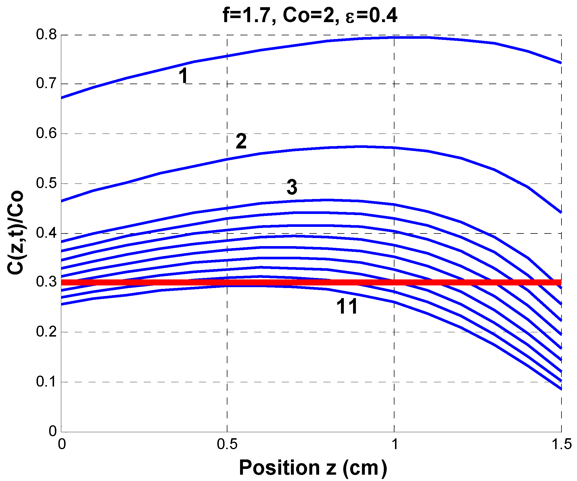
Figure 9 shows the tightly focused case with f = 1.7 cm (less than f*). The polymerization process starts from z = 1.5 cm (at t =38 s) and moves to z = 0.5 cm (at t = 54 s). At the same time, it moves from z = 0 (at t = 48 s) to z = 0.5 cm (at t = 54 s). Similar to the optimal case, the polymerization process stars with both ends, moving to the central area. However, the tightly focused case starts from the bottom (z = 1.5 cm) and moves to the surface (z = 0), whereas the optimal case began at the surface and offers the advantage of a larger polymerization volume at a given time. Greater details will be discussed in the next section.

Figure 8. Same as Figure 7 but for optimal focusing with f = f* = 2.0 cm. Curves 1 to 9 are profiles at t = 15, 30, 40, 50, 52, 54, 56, 58, and 60 s, respectively.

Figure 8. Same as Figure 7 but for optimal focusing with f = f* = 2.0 cm. Curves 1 to 9 are profiles at t = 15, 30, 40, 50, 52, 54, 56, 58, and 60 s, respectively.

The above-discussed polymerization boundaries for various focusing conditions are further demonstrated by Figure 10, which shows the schematics of the time evolution (at t = 50 and 60 s) of photo-polymerization via (1) a collimated beam, (2) a tightly focused beam (with F = L), (3) an optimally focused beam (f = f*), and (4) a mildly focused beam (f = 2L). In the figure, the polymerized portions are shown by shaded areas and the non-polymerized areas are shown in white. This schematic is further interpreted below.

For a collimated beam, the top portion (approximately 0.3 cm) of the medium is always polymerized starting from the surface (z = 0), which has the highest polymerization rate. As shown earlier by Figure 9, after 90 s of laser irradiation, the deep portion (z > 0.6 cm) of the medium is not polymerized.

Figure 9. As Figure 7, but for tighter focusing with f = 1.7 cm. Curves 1 to 9 are profiles at t = 15, 30, 38, 40, 42, 44, 46, 48, 50, 52, and 54 s, respectively.

Figure 9. As Figure 7, but for tighter focusing with f = 1.7 cm. Curves 1 to 9 are profiles at t = 15, 30, 38, 40, 42, 44, 46, 48, 50, 52, and 54 s, respectively.

Figure 10. Schematics of the time evolution of photo-polymerization via (1) a collimated beam, (2) a tightly focused beam (with f = L), (3) an optimally focused beam (f = f*), and (4) a mildly focused beam (f = 2L), where the polymerized portions are shown by shaded areas.

Figure 10. Schematics of the time evolution of photo-polymerization via (1) a collimated beam, (2) a tightly focused beam (with f = L), (3) an optimally focused beam (f = f*), and (4) a mildly focused beam (f = 2L), where the polymerized portions are shown by shaded areas.

For the tightly focused case (with f = L = 1.5 cm), the medium is polymerized starting from the bottom portion, which has a higher laser intensity initially, and therefore, the initiator concentration C(z,t) is depleted faster than in the top portion. For a mildly focused case (with f = 2L > f*, not optimized), the polymerization process of the collimated case is improved, but it is not ideal. At the optimal focusing, with f = f* given by the scaling law, the photo-polymerization process starts from both ends (top and bottom) and gradually moves to the central portion until the whole medium is polymerized.

The tightly focused case (2) in Figure 10 with f = L provides a faster process than the others. However, the optimized case (3) with f = f* provides a larger volume of completed polymerization at a given time. We choose f* as the optimal condition based on not only the uniform polymerization distribution but also on its larger volume than in the tighter focusing case.

5. Conclusions

We have presented comprehensive modeling for the kinetics of photoinitiated polymerization using a UV laser in thick polymer systems in which the photolysis product still partially absorbs the laser after polymerization. We have demonstrated that the focused beam at an optimal condition (f = f*) achieves uniform polymerization and eliminates the intrinsic drawback of a collimated beam in a thick medium. Transient profiles of the initiator concentration at various focusing conditions are analyzed to define the polymerization boundary and to demonstrate the advantage of optimal focusing for more uniform polymerization and a larger volume of polymerization than the collimated or non-optimal cases. Too much focusing (with f < f*) provides for a fast process; however, it has a smaller polymerization volume at a given time than the optimal focusing case. Finally, a scaling law governed by f* = 1.6/(ε₁C₀) is derived numerically and shows that a larger extinction coefficient or a larger initial concentration of the initiator (larger value of (ε₁C₀)) require a tighter focusing or a smaller f*. The scaling law provides useful guidance for the prediction of the photoinitiated polymerization, particularly in thick polymer systems under focused UV laser illumination. The focusing technique also provides a novel and unique means for uniform photo-polymerization (within a limited time of light irradiation), which cannot be achieved by any other means.