Impact of Grass Cover Management with Herbicides on Biodiversity, Soil Cover and Humidity in Olive Groves in the Southern Iberian

Abstract

In the present work, we studied the effect of herbicide use on extensive olive grove cultivation. To carry out this study, we analysed the effect that herbicide use had on biodiversity, vegetation cover and soil water content. For this purpose, 96 vegetation and soil sampling points were first taken, then georeferenced, and for each sampling point, several bioclimatic variables were interpolated. We concluded that the management of cover crops with herbicides over a long period of time resulted in a decrease in biodiversity, and the dominance of some species that were more resistant to herbicides was increased. Another finding was that the vegetation cover was reduced in the resampling in cases with herbicide management and that the location within the cropland (under the tree canopy, road, boundary or pasture) also has an influence. Finally, the study of soil moisture shows that soil water content was lower in the case of management with herbicides than in the case of management without herbicides. This loss of soil moisture was more accentuated and faster in areas with less vegetation cover. This work highlights the need to change the management models for tree crops in order to preserve biodiversity, soil quality and optimise water resources in a context of accelerated climate change in one of the regions most severely affected by global warming, the Mediterranean belt.

1. Introduction

The Mediterranean region is highly vulnerable to global warming and is suffering a significant decline in rainfall, and hence a decrease in available water resources in the circum-Mediterranean region [1]. Due to its location and complex orography, the Iberian Peninsula has a very variable climate [2,3] and is particularly susceptible to climate change. Although rainfall distribution is not homogeneous in all areas and depends on several geographic factors [4,5,6], it is clearly necessary to find strategies to optimise rainfed and irrigated crops in these regions. In the Mediterranean region, the southern Iberian Peninsula is renowned for its agricultural activity in general and olive groves in particular. To this end, we analysed the impact of the management of grass cover in the period spanning 2006–2016.

In Spain, 2.584.564 ha. of olive groves were cultivated in 2013, representing 60% of European Union production and 45% of world production [7]. These extensive crops pose a high demand for water resources and require improved management of surface water, to avoid depending on groundwater, not only in growing crops but also for grazing needs [8,9].

Another problem associated with global warming is the rise in natural disasters as a result of the more frequent occurrence of torrential rainfall [10,11], causing a loss of unprotected soils. Soil loss due to human actions in olive groves in Andalusia is estimated at an average of between 29 and 47 tonnes/hectare per year and ranges to over 100 tonnes in olive groves in southern Spain [12]. This erosion leads to degradation and the loss of the characteristic attributes of productive and cultivable soil, rendering it sterile for agricultural purposes [13], reducing the soil water retention capacity and leading to the emergence of badlands [14] and tillage soil [15], all of which causes significant economic costs at a global level [16].

The Sustainable Development Goal (SDG) indicators set out the objectives for sustainable development for 2030. This objective specifically proposes to protect, restore and promote the sustainable use of terrestrial ecosystems and forest management, combat desertification, and halt and reverse land degradation and biodiversity loss. Goal 15.9 is related to integrating ecosystem and biodiversity values into national and local planning, development processes, poverty reduction strategies and accounts [17].

Several mechanisms have been developed over time to improve the use of water resources [18,19]. One of the solutions for ensuring soil water availability and preventing erosion is to grow crops with natural vegetation cover [4,20] and improve crop management using bioclimatic approaches [21]. Other solutions for ensuring soil water availability and preventing erosion are to grow crops with natural vegetation cover, with particular attention on the enhancement of the crop’s wild relatives especially if seen as a priority [22]. To contextualize the importance of grass communities in crops, it is worth noting that the Mediterranean basin is characterised by a high density of grass species (around 120–180 species/1000 m² and 40–60 species/m²), of which more than 70% correspond to annual therophytes. These plant formations, therefore, represent one of the most diverse types of vegetation in the temperate zone [23,24,25].

These proliferations of species are perfectly adapted to the rigours of the Mediterranean climate [26] and can, therefore, compete with crops. On the other hand, these plant communities are deeply related to the nutritional status of the soil, and it is these variables in the nutritional composition of the soil that largely determines the presence or absence of certain characteristic species. Thus, several studies propose methodologies to evaluate the nutritional composition of the soil based on the floristic composition of the plant communities [27].

In the case of olive groves, these herbaceous communities may represent a problem when the olive grove is young; that is, in the first years of implantation. Various techniques have been used for decades to eliminate these natural plant covers, such as chemical mowing pre- and post-emergence with the use of herbicides [28]. This continuous use of herbicides—especially pre-emergence—depletes the soil’s seed bank, which in many cases leads to a reduction in biodiversity [29] and the complete disappearance of the plant cover, leaving the soil totally unprotected against erosion [30].

The main aim of this present study is to analyse the impact on the soil water retention capacity induced by the loss of natural vegetation cover in a gradient of human intervention reflected in the location of the sampling points in olive groves in the southern Iberian Peninsula over the 2006–2016 period.

The first hypothesis in this work is that the use of herbicides transforms the floristic composition of the various types of plant communities growing in olive groves and that these changes respond to a combination of soil and bioclimatic parameters that are exclusive to each plant community. Another starting premise is that the more stenoic and exclusive species in each plant community are replaced by more generalist and eurioic species.

Another working hypothesis is that under a Mediterranean bioclimate, the dry period coincides with the withering of the plant cover, which, if the soil is bare, causes greater water loss than in places where there are remnants of plant cover. Furthermore, the present work aims to analyse the effect of the continued use of herbicides, both pre-and post-emergence, and of plant cover management using mechanical treatments (mechanical reaping and grazing) on the floristic composition of the various types of plant communities growing spontaneously in olive groves in the southern Iberian Peninsula.

2. Materials and Methods

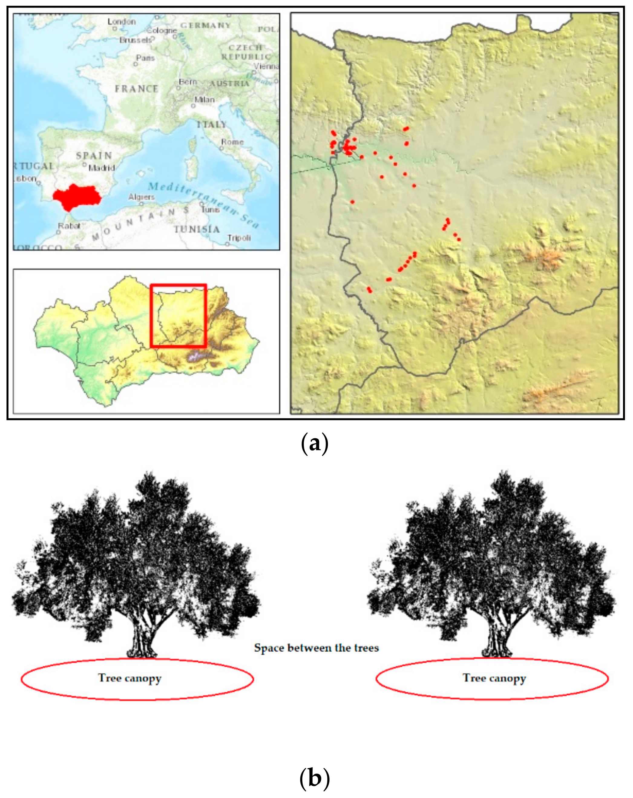
2.1. Study Area

The study area includes the sampling points established in the spring of 2006 [31] in the NW of the province of Jaén and the NE of the province of Córdoba, in the Region of Andalusia in the southern Iberian Peninsula (Lat. 37°56′ N; Long. 4°3′ W). A total of 91 points were visited during the spring of 2016 in the countryside of the Guadalquivir Valley and Sierra Morena (Figure 1a). The sampling points were distributed in agricultural areas of olive groves and grass-covered areas of pastureland (dehesa) to contrast 2 different methods of managing the vegetation cover over 2006–2016. All of the sampling points were located in open areas with no dense trees, and the sampling points in the olive groves were distributed in the centre between 2 trees and near the tree canopy (Figure 1b).

The altitudinal range extended from 176 m asl to 638 m asl, with an average slope of 8.01°. The orientation of the sampling points was predominantly south–southwest. The values of altitude, inclination and orientation were obtained from the digital terrain model with a mesh pitch of 100 metres.

2.2. Sampling and Resampling Points

In the spring of 2016, 91 points were resampled. These points had previously been sampled by Cano-Ortiz in 2006 [31]. The samples were classified according to their location in the different study plots following a gradient of human influence on grassland management from highest to lowest:

—

Immediately under the olive tree canopy

—

In the middle of the road (outside the canopy)

—

On the fringe of the olive grove

—

Dehesa

Two types of weed management were selected: Olive groves in which the vegetation cover was continuously treated without the use of herbicides (no herbicides) by means of an alternative control of the herbaceous cover once it had withered. The other type of locality corresponded to olive groves with continuous use of the herbicides oxyfluorfen at 24% (3 L/ha) and glyphosate at 36% (4 L/ha) over the last 10 years. The applied concentration was as recommended on the herbicide label. To control the shoots from the olive tree trunks, formulations based on glyphosate at 36% were applied at the base of the tree trunk.

2.3. Climatic and Bioclimatic Data

Each sampling point was georeferenced by means of UTM coordinates and was associated with different bioclimatic, soil and geographic parameters. The temperature and precipitation parameters were obtained through interpolation in a neural network trained by the Neuraltools^® package from 2434 weather stations in the Andalusian region belonging to the National Meteorological Agency (AEMET) and the Climate Information System of the Andalusian Regional Government. For each sampling point, the neural networks were established for each climate variable (maximum, average, minimum temperature and rainfall) for each month of the year. The climate and bioclimatic variables were defined following the criterion of Rivas-Martínez [32]. The following climate variables were considered for the present study:

• T: Mean annual temperature in degrees centigrade
• M: Mean temperature of the maximums
• m: Mean temperature of the minimums
• Tmax: Mean temperature of the warmest month of the year
• Tmin: Mean temperature of the coldest month of the year
• Tp: Positive annual temperature (sum of the months with a mean temperature above 0 °C in tenths of degrees centigrade)
• Pp: Positive annual precipitation (of the months in Ti above 0 °C)
• PE: Thornthwaite’s potential annual evapotranspiration index [33]
• PEs: Potential evapotranspiration index of the summer quarter
• PE_1–12: Potential monthly evapotranspiration index 1 = January, 2 = February, … 12 = December

Bioclimatic variables used:

Annual aridity index (Iar);

$$Iar=\frac{PE}{P}$$

Diurnality index (Id): The difference between the mean maximum temperature (Tcmax) and the mean minimum temperature (Tcmin) of the months with the greatest temperature differences in the year; that is, the month with the greatest daily swing or interval between the maximum and minimum temperatures.

$$Id=Tcmax-Tcmin$$

Humidity index: The percentage of precipitation above or below the annual precipitation (P) compared to the annual evapotranspiration (PE)

$$IH=100\ast \frac{\left(P-PE\right)}{PE}$$

Mediterraneity index (Im): The coefficient between the value for Thornthwaite’s mean summer evapotranspiration (PEs), and precipitation in mm in the same period (Ps).

$$Im=\frac{PEs}{PS}$$

Mediterraneity index for the month of July (Im₁) and for July and August (Im₂);

$$I{m}_1=\frac{PE{s}_7}{P{s}_7}; I{m}_2=\frac{PE{s}_{7–8}}{P{s}_{7–8}}$$

Annual evapotranspiration index (Ioe): The coefficient between mean precipitation (P) and potential annual evapotranspiration (PE, Thornthwaite).

$$Ioe=\frac{P}{PE}$$

Ombrothermic index of the warmest month of the summer quarter (Ios1); ombrothermic index of the warmest 2 months of the summer quarter (Ios2), ombrothermic index of the summer quarter (Ios3), and ombrothermic index of the summer quarter and the previous month (Ios4).

$$Io{s}_1=10\ast \frac{P_{warmest month}}{T_{m warmest month}}; Io{s}_2=10\ast \frac{P_{warmest two months}}{T_{warmest two months}}; Io{s}_3=10\ast \frac{P_{6–8}}{T_{6–8}}; Io{s}_4=10\ast \frac{P_{5–8}}{T_{5–8}}$$

Monthly ombrothermic indices (Iom_1–12); with i = 1 = January, 2 = February, …, 12 = December.

$$Io{m}_i=\frac{P_i}{T_i}$$

Annual ombrothermic index (Io); the coefficient between the total mean precipitation in mm in the months with a mean temperature above 0 °C (Pp) and the sum of the mean monthly temperatures above 0 °C in tenths of a degree (Tp).

$$Io=\frac{Pp}{Tp}$$

Simple continentality index (Ic): The continentality index expresses in degrees centigrade the difference or oscillation between the mean temperature of the warmest month (Tmax) and the mean temperature of the coldest month of the year (Tmin).

$$Ic=Tmax-Tmin.$$

Thermicity index (It): This index describes the intensity of cold, which is a limiting factor for many plants and plant communities.

$$It=\left(T+m+M\right)10$$

To weigh the excess of cold or thermicity in the most continental or oceanic locations in areas located north or south of parallel 230°, a compensation factor C was added to the It value based on the continentality values in the area: Itc = It + C. (

Table 1. Calculation of the compensation value of C for the calculation of ITC (Compensated thermicity index), based on the Ic value.

Ic Value	C Value
≤8	C = (Ic − 8) × 10
8 < Ic ≤ 18	C = 0
18 < Ic ≤ 21	C = (Ic − 18) × 5
21 < Ic ≤ 28	C = (Ic − 21) × 15
28 < Ic ≤ 46	C = (Ic − 28) × 25
46 < Ic ≤ 65	C = (Ic − 46) × 60

).

The figures for altitude, orientation and slope were obtained by plotting the previously georeferenced points on a digital terrain map (DTM) with a pixel resolution of 10 × 10 metres. The numerical values for altitude, orientation and slope were obtained from the DTM for each sampling point.

2.4. Soil Data and Moisture

The soil data for each sampling point were recorded in a Geographic Information System (GIS). These data were taken from Cano-Ortiz [31].

In order to observe the effect of different vegetation covers on soil moisture, the amount of water in the soil was measured at 100, 200, 300 and 400 mm with 3 repetitions for each depth; this was done continuously over the months of the highest rainfall in the Mediterranean macrobioclimate (spring and autumn) in an olive grove located in the centre of the total study area. These measurements were taken in areas with 0 (bare soil), 5, 25, 50, 70, 85, 90, 95 and 100% cover, performing a maximum of 5 and a minimum of 3 repetitions for each cover (some measurements had to be eliminated due to reading errors or failure of the probe). The measurements were taken with the Delta-T Profile probe PR-1 device and on slopes between 0 and 10°.

Once the influence of the cover on the soil water retention capacity was calculated by linear regression, the results were interpolated to the rest of the sampling points from the cover and slope values.

2.5. Determination of the Flora and Delimitation of the Plant Communities

The flora was identified following reference works such as Flora Ibérica [34], Flora de Andalucía Oriental [35] and Flora de Andalucía Occidental [36]. Monographs and specific works were consulted for certain problematic taxonomic groups such as the genus Taraxacum [37]. The monograph by León E. et al. [38] was consulted for the genus Hordeum. The work by Devesa et al. was followed for Gramineae in general [39].

The phytosociological model was used to carry out the vegetation sampling, estimating the cover by means of the Braun-Blanquet [40] method and transforming the phytosociological cover indices (5, 4, 3, 2, 1, “+”, “r”) into numerical indices according to

Table 2. Conversion of the values of the phytosociological indices and their correspondence with the average percentage cover values. The non-numerical values (“+” and “r”) have been transformed and estimated by interpolation from the numerical indices (the transformation of the phytosociological are according to [26,42]).

Phytosociological Index	% of Average Cover
5	85
4	65
3	45
2	25
1	12
+	6
r	3

. The phytosociological and syntaxonomical descriptions of the plant communities in the study were included and named according to Rivas-Martínez [41].

2.6. Data Analysis

The qualitative and quantitative relationship between the relevés in both sampling periods was first verified to establish a correlation between the samples taken in 2016 and 2006. This was done by designing a matrix in which the columns represented the sites or sampling plots, and the rows contained the different taxa samples. A multiple correlation analysis was subsequently established to obtain a correlation coefficient between each pair of relevés and the p-value for the significance of the correlation, using the EXCEL extension XLSTAT (Version 2014.5.03). The matrix of correlation coefficients was in turn obtained from a matrix of covariances with the following equation:

$$\frac{C_{i,j}}{\sqrt{C_{i,i\times C_{j,j}}}}$$

where C represents the covariance value. The matrix of p-values was obtained to verify the hypothesis of a correlation between the different relevés. The p-value was calculated by converting this correlation matrix into a t statistic with N − 2 degrees of freedom, where N was the total number of taxa sampled in the 2 time periods, and R was the correlation coefficient; the confidence intervals were based on a normal asymptotic distribution of:

$$0.5\times Log\left(\frac{1+R}{1-R}\right)$$

and with a variance approximately equal to 1/(N − 3).

The changes in the floristic composition of the plant communities in the vegetation cover of the olive grove and dehesa over 10 years were analysed using Shannon’s diversity index [43], the evenness index [44] and Simpson’s dominance index [45], comparing the evolution of these values in both time periods.

For a better characterisation of the plant communities in the vegetation covers, factor analysis was first performed to gain a better understanding of the soil and bioclimatic variables involved in the composition and structure of the grassland communities in the olive groves in the southern Iberian Peninsula. This factor analysis was performed with the soil variables for each sampling point, and the interpolation of the bioclimatic variables obtained previously.

The data were standardised prior to the statistical or ordination analyses using the following formula:

$$X^{\prime }=\frac{X-\mu }{\sigma }$$

where X is the value of the variable, µ is the mean and σ is the standard deviation.

A Shapiro–Wilk normality test was first done to confirm that the data met the assumptions that ensure the reliability of the ANOVA test. An analysis of variance (two-way ANOVA) was performed to study the effects of the location and the plant cover treatment on the plant associations assessed in the 2 time periods and the interaction of the treatment, location and association variables. In this case, a multivariate analysis of variance (MANOVA) was used.

After normalising the data in the matrix, a factor analysis was performed. Factor analysis is a multivariate analysis method aimed at studying the relations of interdependence between a set of variables or individuals. The criterion for the choice of bioclimatic variables was chosen after rotating the factor matrix by means of the VARIMAX algorithm and transforming the initial factor matrix into a rotated factor matrix to make it easier to interpret. This procedure was done only for the bioclimatic and soil variables. The bioclimatic variables selected had a correlation of over 95% with the other factors, and the soil variables had a correlation of over 80%. With the previously selected variables, a CCA (Canonical Correspondence Analysis) was performed to see which climatic and edaphic variables were involved in the co-occurrence of the different species in the sampling points.

3. Results

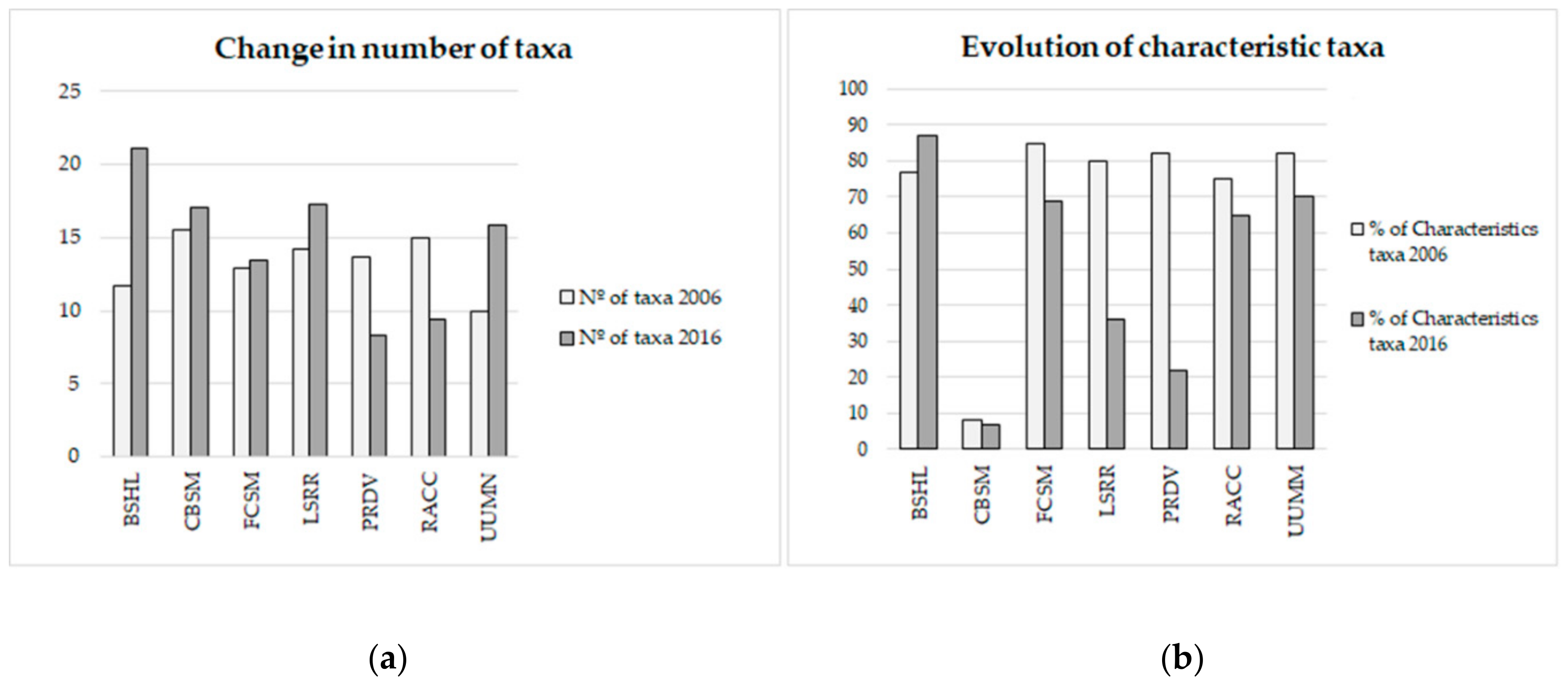
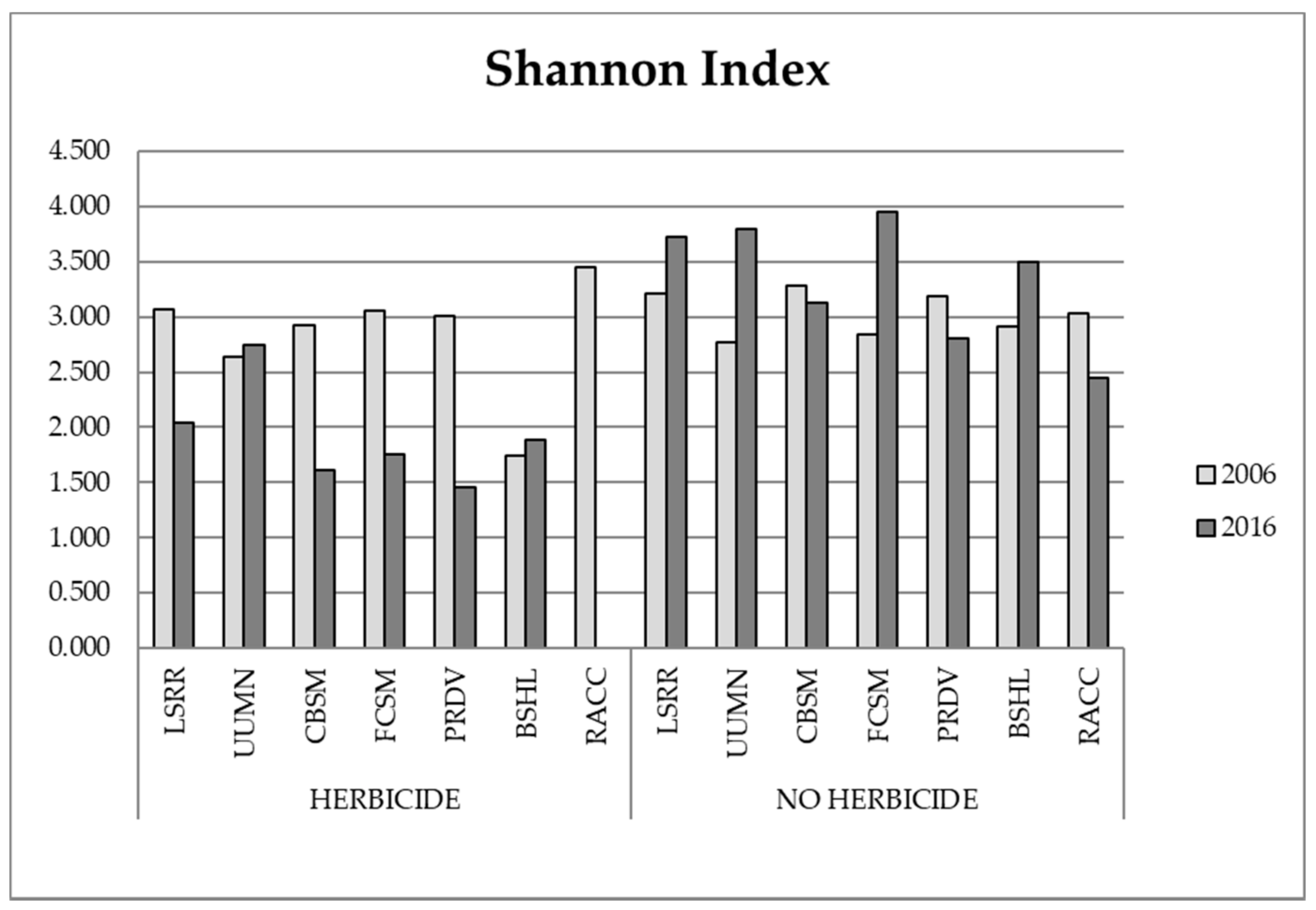
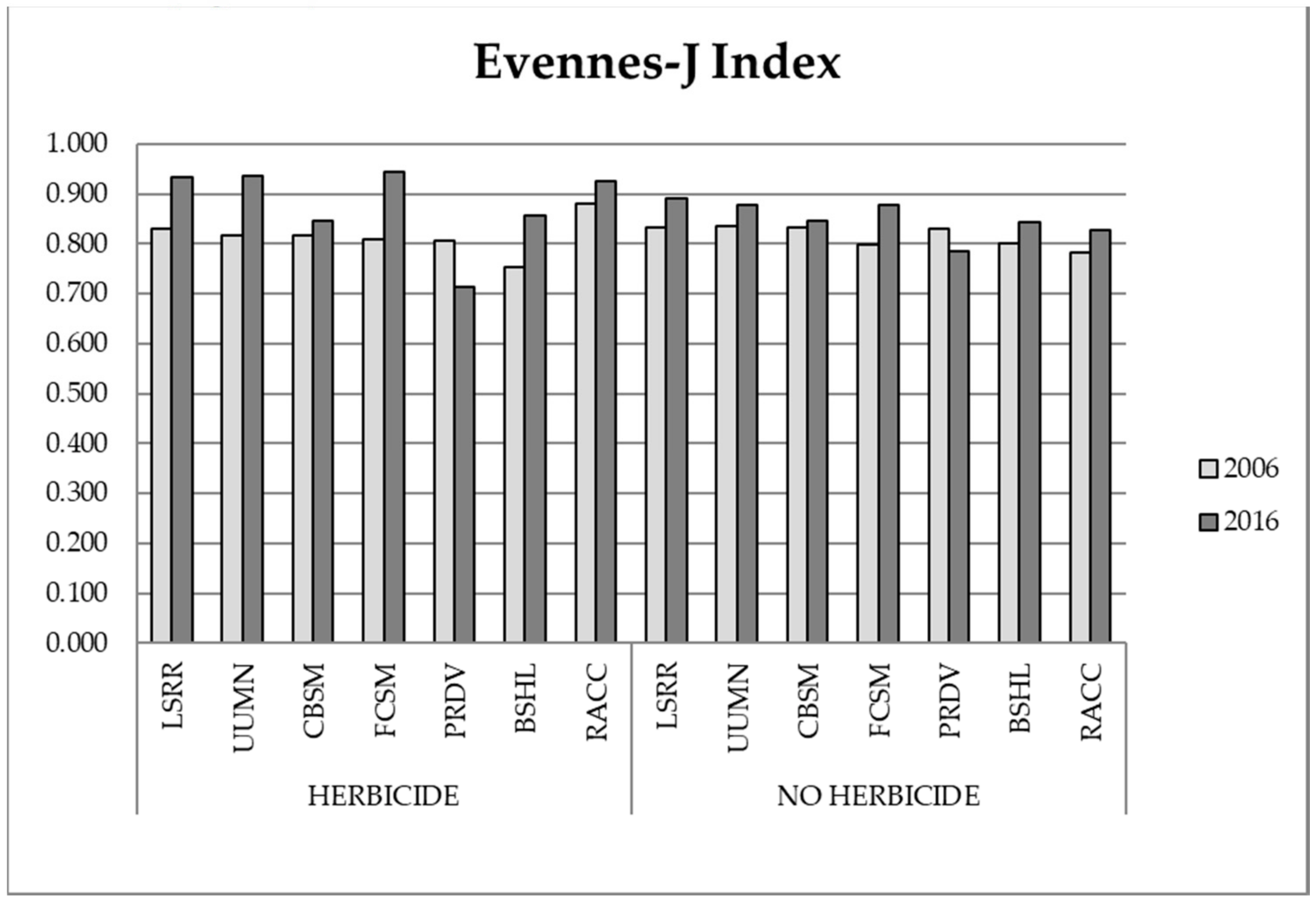
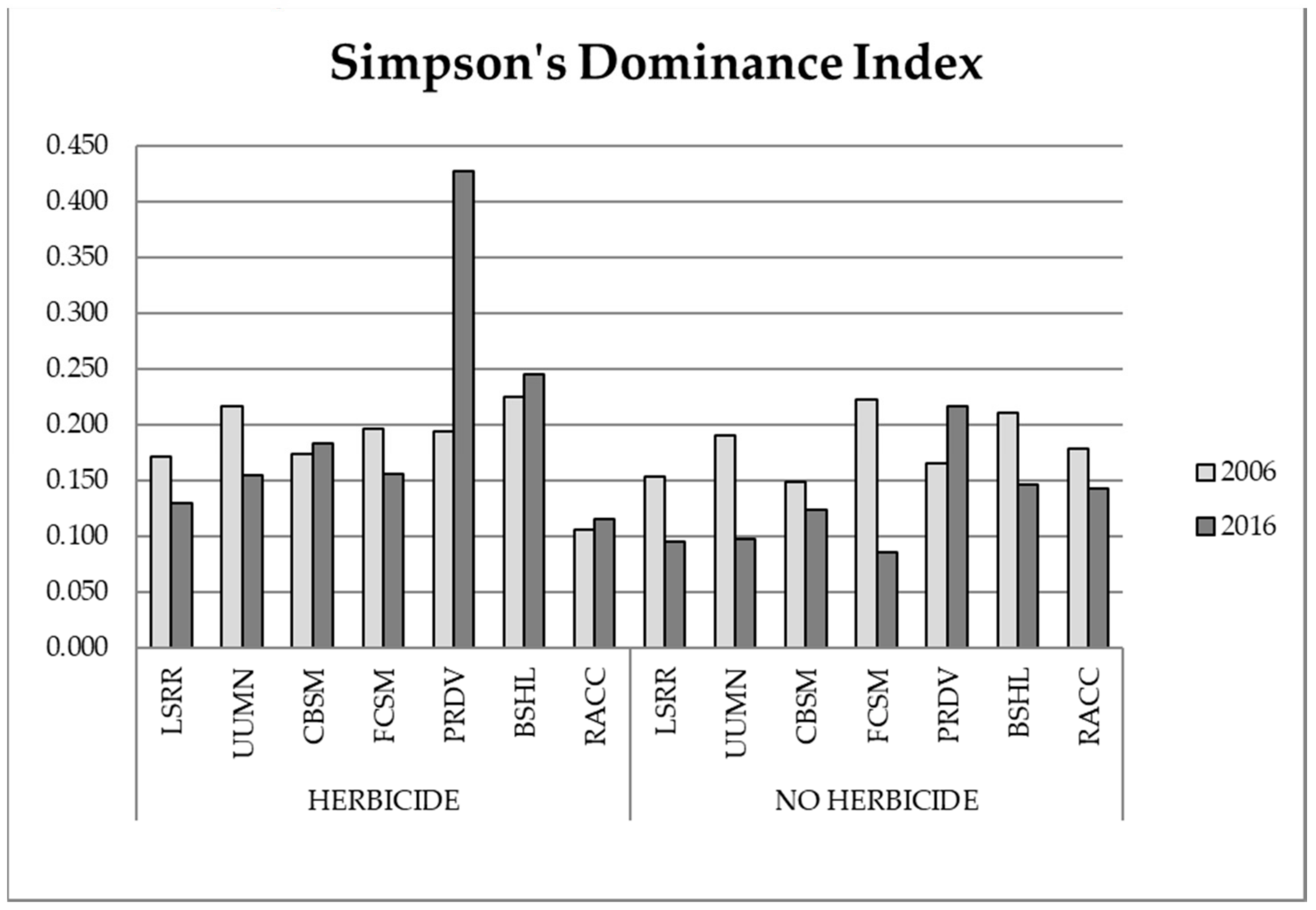
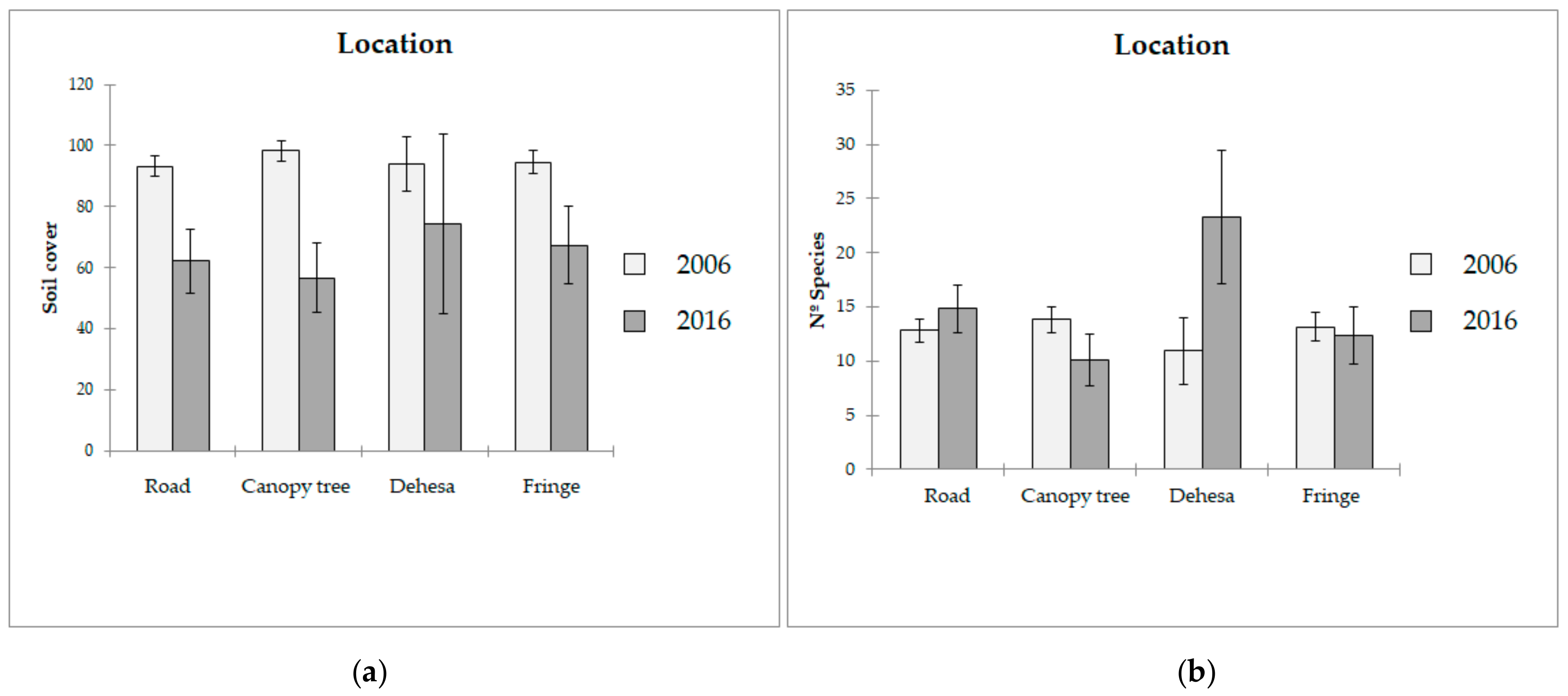
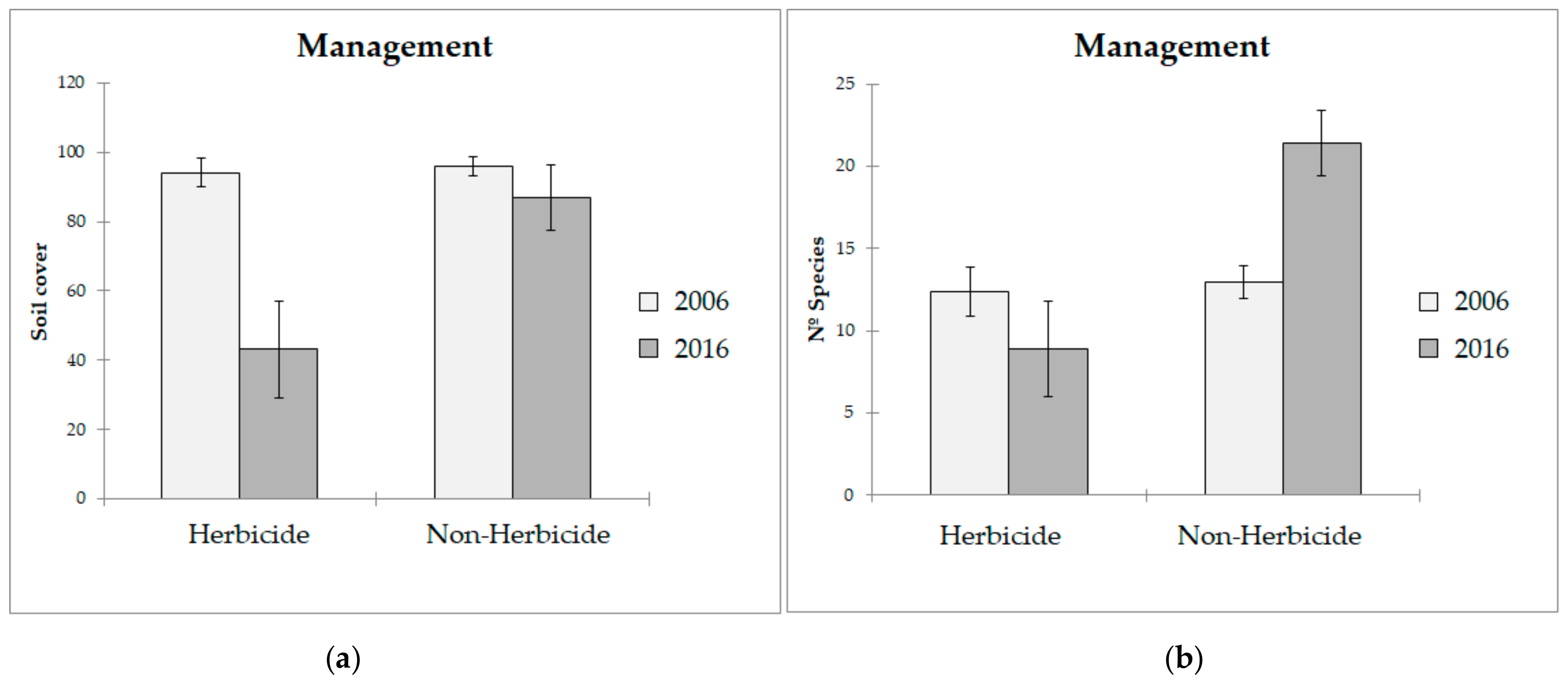
3.1. Biodiversity Analysis

A number of 283 taxa in the ranks of species, subspecies and variety were detected in the 91 sampling points in 2016. All species determined were angiosperms, of which 15.36% were monocotyledoneae, forming 4 of the 39 botanical families detected. The remaining 84.64% were dicotyledoneae, accounting for 31 of the 39 families detected; 66% of these species were represented by 5 botanical families: Asteraceae, Fabaceae, Poaceae, Caryophyllaceae and Brassicaceae, and to a lesser degree the family Apiaceae. Such is the plant diversity that just 7.6% of the total flora present in eastern Andalusia was detected in the 91 sampling points (the total area of all the sampling points was 150 m²) [35].

A more detailed analysis of the changes in floristic composition for each community in the study showed that the number of taxa did not change homogeneously but depended on the type of community in which the samples were taken in 2016 compared to 2006 (Figure 2a,b).

The analysis of alpha diversity (evaluated using the Shannon index) showed that there were no significant differences (Figure 3) in diversity in the management of plant cover with and without herbicides in 2006 (p-value = 0.5928), regardless of the location of the sampling point. In the sampling of these same points in 2016, it can be seen that the alpha diversity had increased at points where the herbaceous cover was managed without herbicides; while the points where the cover had been managed with herbicides continuously over 10 years had undergone a very significant (p-value < 0.001) decrease in alpha diversity.

The communities in the vegetation covers (Figure 4) that can be said to be most affected by the treatment with herbicides are Carduo bourgaeani-Silybetum marianum (CBSM) (p-value = 0.0149), Fedio cornucopiae-Sinapietum mariei (FCSM) (p-value = 0.0243), Resedo albae-Chrysanthemetum coronarii (RACC) (p-value < 0.001) and Linario spartei-Raphanetum raphanistri (LSRR) (p-value = 0.0238), which saw a significant decrease in alpha diversity D between 2006 and 2016. In the management without non-herbicide of herbaceous covers, the associations Urtico urentis-Malvetum neglectae (UUMN) (p-value = 0.0215), Bromo scopariae-Hordeetum leporini (BSHL) (p-value = 0.0435) and FCSM significantly increased in terms of biodiversity (p-value = 0.0178).

The evenness index showed how evenly individual species were distributed within a community. Values close to 1 showed that the area occupied by each species within the sampling area was similar, while low evenness values indicated that the numbers belonging to individual species represented in the community were heterogeneous. In this case (Figure 3), no significant differences could be seen between the evenness indices in 2006 in the management with and without herbicides. Nor were there any significant differences between the two management types in the 2016 resampling.

The analysis of the evenness index by the community in samples where the grass covers were managed with herbicides in both the 2006 and 2016 samplings showed that there were significant increases in LSRR (p-value = 0.356), UUMN (p-value = 0.476) and FCSM (p-value = 0.217), indicating that the communities tended to be homogeneous and that all species were represented more homogeneously. For communities with non-herbicide management, there were no significant differences in the evenness index between 2006 and 2016 (Figure 5).

The Simpson dominance index measures how likely it is that two individuals selected at random are from the same species. Values close to 1 indicate that there is a high representation of only a few species that are, therefore, dominant in the community. This analysis shows that there were no significant differences between herbicide and non-herbicide cover management styles in the 2006 samples. However, in the 2016 resampling, increased dominance of a few species was found in points where the grass cover was managed with herbicides, indicating that continuous treatment with herbicides caused a selection of more resistant species which dominate in the community (Figure 3).

The analysis of the Simpson dominance index for each plant community observed in the two management types (Figure 6) revealed that the most affected community was Papaverido rhoeadis-Diplotaxietum virgatae (PRDV) with a significant difference (p-value < 0.001). The dominance index decreased significantly in the UUMN as-sociation (p-value = 0.0105). The comparison of points sampled in 2006 and points resampled in 2016 with non-herbicide grass cover management showed a significant decrease in Simpson’s dominance index in FCSM (p-value = 0.0188), UUMN (p-value = 0.0097), LSRR (p-value = 0.023) and BSHL (p-value = 0.0436), indicating that species that were previously underrepresented in non-herbicide managed sampling in 2006 points were now better represented within the community.

As can be seen in Table 2, the result of the MANOVA analysis indicated that there were significant differences in biodiversity indices between the associations and in the type of management of the herbaceous cover in each plant community. The location of the sampling points, the management of the herbaceous cover itself and the interactions between location/association, location/treatment/association were not significant. It is, therefore, the grass cover management in each association that significantly influenced the changes in plant communities.

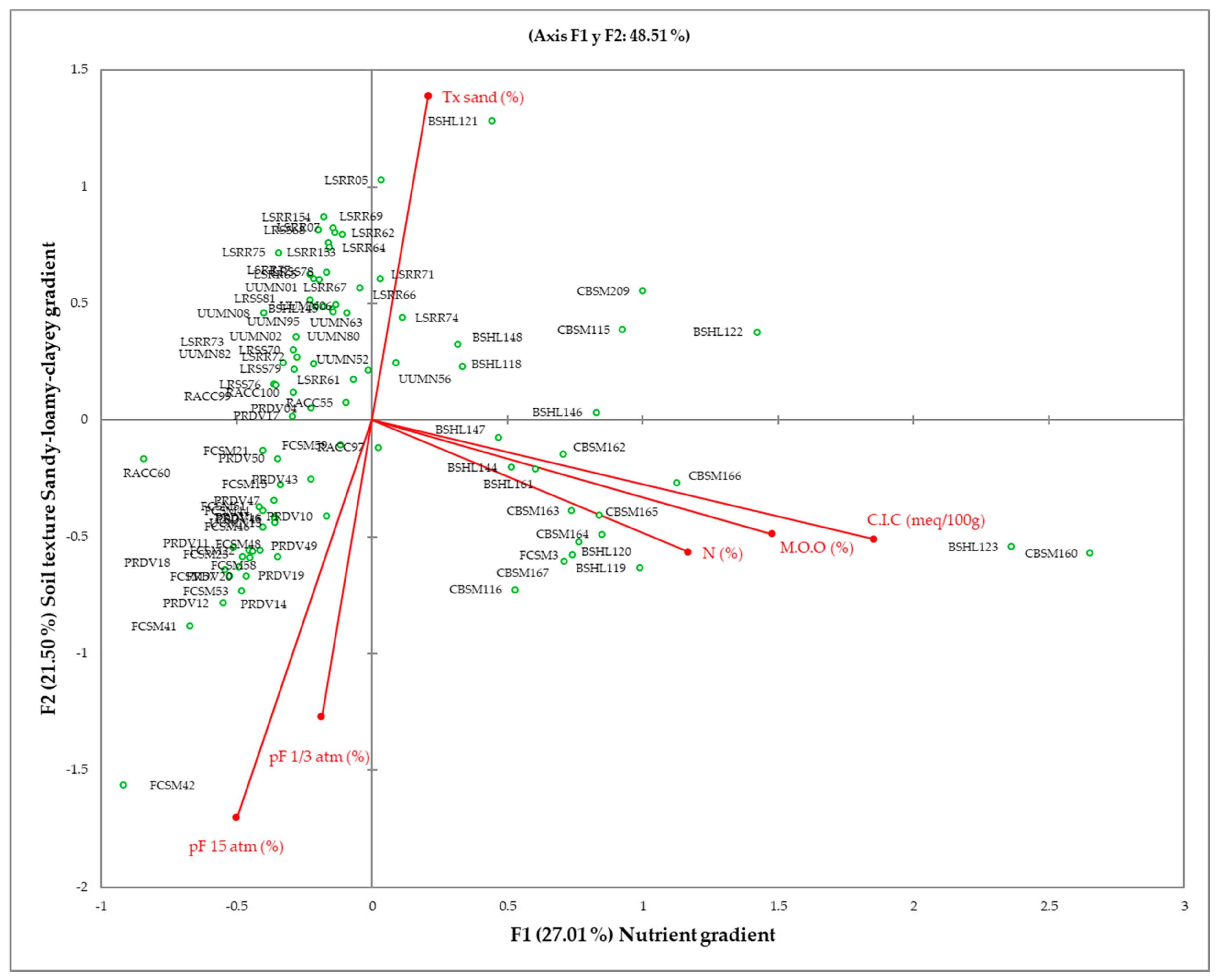
3.2. Soil and Bioclimatic Characterization of Plant Communities

Table 3. Multivariate analysis of variance (MANOVA) showing which independent variables underwent changes: Location (tree canopy, road, fringe and dehesa), management (herbicide, non-herbicide), type of association (BSHL, CBSM, FCSM, PRDV, UUMN, LSRR or RACC) or a combination of these can influence the dependent variables (biodiversity indices in this case). In bold, significant values at 95% confidence.

	Location	Management	Association	Location/Management	Location/Association	Management/Association	Location/Management/Association
Lambda	0.7227	0.9511	0.2358	0.8167	0.4691	0.5699	0.8921
F (Observed values)	0.9782	0.4367	2.0845	1.9077	0.8834	1.7684	1.0282
GL1	18.0000	6.0000	42.0000	6.0000	48.0000	18.0000	6.0000
GL2	144.7351	51.0000	242.6633	51.0000	255.0037	144.7351	51.0000
F (Observed values)	1.6755	2.2826	1.4350	2.2826	1.4080	1.6755	2.2826
p-value	0.4880	0.8509	0.0003	0.0974	0.6905	0.0345	0.4179

shows the factor analysis carried out to determine which soil variables conditioned the floristic composition of the plant communities. The highest factor weightings after the VARIMAX rotation were observed in cation interchange complex (C.I.C.), oxidizable organic matter (M.O.O.), nitrogen (N), water potential at 1/3 atm. (pF 1/3), water potential at 15 atm. (pF 15) and sandy soil texture (Tx sand), with correlation values higher than 0.8. Similarly, the bioclimatic variables best related to the floristic composition of the plant communities studied were the aridity index (Iar), humidity index (IH), summer ombrothermic index (Ios), ombrothermic index (Io), evapotranspiration (PE), summer evapotranspiration (PEs), and April, May and August evapotranspiration (PE₄, PE₅, PE₈). As can be seen in

Table 4. Correlation with the first two axes (F1 and F2 explained the higher variability found in the first two axes of the factor analysis; F1 = 23.75% and F2 = 21.80% in the soil variables, and F1 = 54.91% and F2 = 37.07% in the bioclimatic variables). Absolute correlation values over 0.8 have been considered for the soil variables, and absolute correlation values higher than 0.95 for the bioclimatic variables. The variables selected are shown in bold.

		Correlation F1	Correlation F2			Correlation F1	Correlation F2
Edaphic variables	C.I.C (meq/100 g)	−0.0394	0.8076	Bioclimatics variables	Iar	0.9785	0.7685
	Carbonates (%)	0.0011	0.4411		Id	−0.9122	−0.8940
	Ca (meq/100 g)	−0.0758	0.4859		IH	−0.9779	−0.7700
	P assimilable (p.p.m)	0.0007	0.7312		Ioe	−0.9779	−0.7700
	Mg (meq/100 g)	0.6487	−0.1194		Ic	−0.8990	−0.9017
	M.O.O. (%)	0.1588	0.8624		o	−0.9631	−0.7961
	N (%)	0.1034	0.8563		It	0.9234	0.8834
	pH 1/2.5	−0.0896	0.1262		Itc	0.9234	0.8834
	K (meq/100 g)	0.3419	0.3974		PEs	0.9587	0.7198
	pF 1/3 atm (%)	0.8825	0.0462		PE4	0.9532	0.8381
	pF 15 atm (%)	0.8966	−0.0460		PE5	0.9624	0.7354
	Tx clay (%)	0.4742	−0.0703		PE6	0.9442	0.6733
	Tx sand (%)	−0.8644	−0.0146		PE7	0.9432	0.6571
	Tx slime (%)	0.6321	0.1294		PE8	0.9640	0.7986
	Sieve 2 mm (%)	0.4172	0.1738		PE9	0.9278	0.8751
	Salinity (mmhos/cm)	0.2863	0.3869		PE10	0.8816	0.9021

, the bioclimatic variables related to water availability had the greatest influence over the presence of these herbaceous communities in the olive groves in the southern Iberian Peninsula.

Canonical correspondence analysis (CCA) (Figure 7) revealed which soil parameters defined the plant communities in the herbaceous cover. As can be seen in Figure 6, the horizontal axis can be interpreted as a gradient of nutrient enrichment in the soil, and the communities that required more N, M.O.O. and C.I.C. were CBSM and BSHL; while the communities with lower nutrient requirements such as PRDV and FCSM were at the opposite end. This axis represented 27.01% of the explained variability. The vertical axis can be interpreted as a soil texture gradient; clay soils show pF1/3 and pF15 for clay soils were higher than for sandy textured soils. There was a preference for sandy soils in the floristic composition of LSRR, as in the case of UUMN, but to a lesser extent. In contrast, in addition to the abovementioned preference of these two types of plant communities, FCSM and PRDV also have appetites for clayey and slightly saline soils. This vertical axis explained 21.5% of the variability.

The unrestricted inertia of the CCA was 9.31%, while the restricted inertia of the model was 90.69%. The permutation test shows that with a p-value < 0.0001, the floristic composition of the plant communities was linearly related to the data on the soil variables.

3.3. Soil and Bioclimatic Characterization of Plant Communities

The analysis of how the different vegetation covers were managed according to the location within the sampling area (tree canopy (p-value < 0.001), road (p-value = 0.0042), fringe (p-value = 0.0208), dehesa (p-value = 0.0870) revealed significant differences in the vegetation cover (Figure 8a). As can be seen, in 2006, the vegetation cover was similar in the different sampling locations with no significant variations. In the 2016 resampling, a significant decrease was observed in all locations except in dehesa, and there was a gradient from fringe to the road with an increase in human activity in the management of the vegetation cover (dehesa cover < fringe cover < road cover < tree canopy cover). Similarly, the number of different species depending on the location of the sampling (Figure 8b) did not vary significantly in the fringe and road locations between the 2006 and 2016 surveys. There were significant differences for the number of species in the tree canopy location (p-value = 0.0390) between the two periods for dehesa, p-value = 0.0019.

The analysis of the grass cover in terms of its management showed that in 2006 there were no significant differences between herbicide- and non-herbicide-managed samples. In 2016, after 10 years of continuous management with herbicides, a significant decrease was observed in the vegetation cover in resampling points where the grass cover was managed with herbicides. There were no significant differences in cover with respect to 2006 in sampling points where the grass cover was managed without herbicides (Figure 9a).

The analysis of the number of species according to the vegetation cover management showed a sharp decline at the points managed with herbicides in the 2016 resampling compared to 2006. At points managed without herbicides, the number of species increased over the 10-year period with respect to 2006 (Figure 9b). A comparison of the two graphs shows that the greatest contribution was from the sampling carried out in the dehesa.

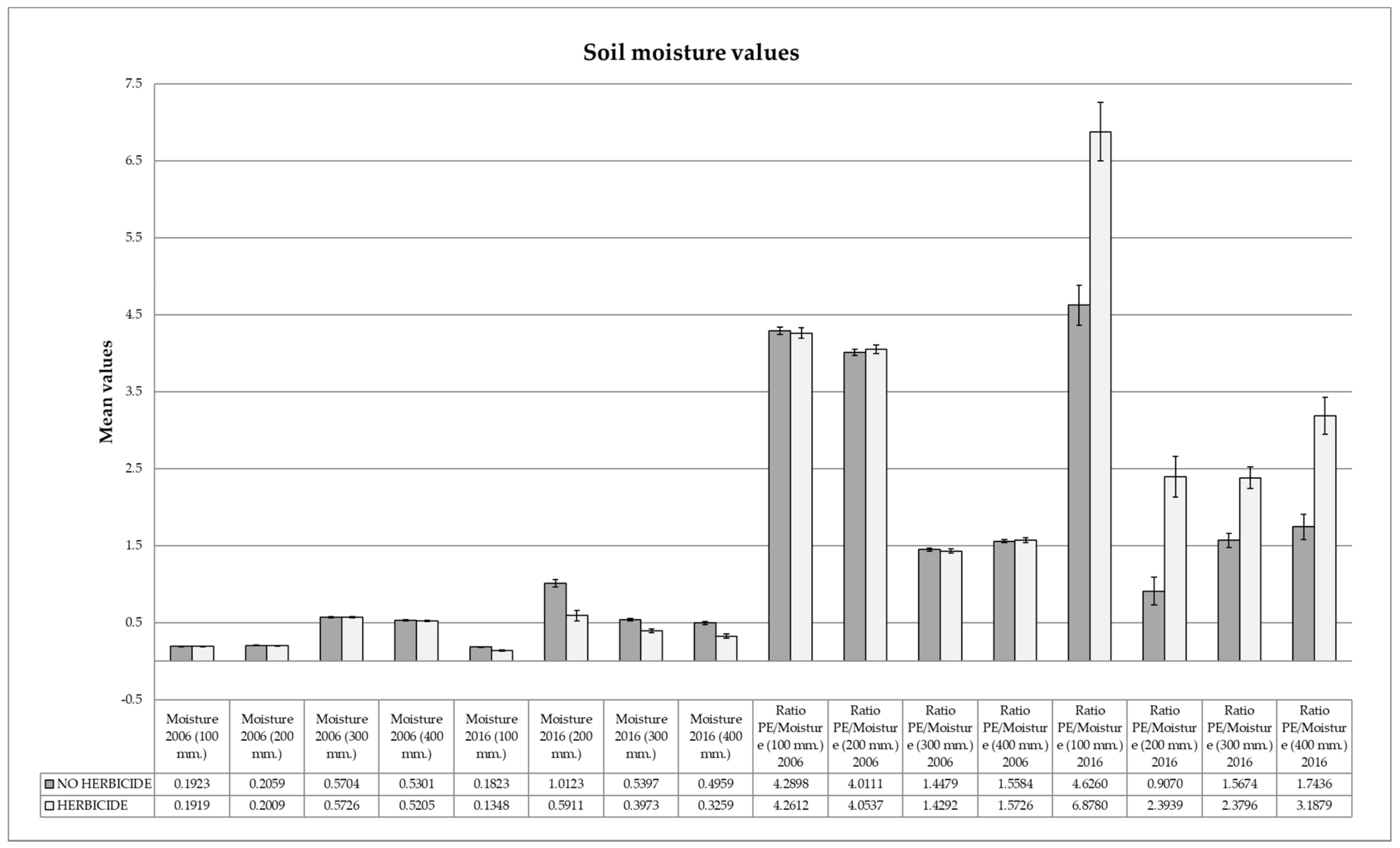
3.4. Soil Moisture Analysis

The analysis of soil moisture revealed significant differences at 100, 200, 300 and 400 mm in depth according to the type of cover management (herbicides vs. no herbicides) in the 2016 resampling (

Table 5. Significance values (p-values) of the analysis of variance between the interactions of location and management variables of herbaceous covers for each soil moisture and PE/soil moisture ratio measurement in each period of analysis over 2006–2016. Significant values with 95% confidence are shown in bold.

			Location						Grass Cover Management
Variables	Mean	Standard Deviation	Road vs. Tree Canopy	Road vs. Dehesa	Road vs. Fringe	Fringe vs. Tree Canopy	Fringe vs. Dehesa	Dehesa vs. Tree Canopy	Herbicide vs. No Herbicide
Soil Moisture 2006 (100 mm.)	0.1917	0.0104	0.0054	0.3833	0.2411	0.1733	0.7999	0.6092	0.8754
Soil Moisture 2006 (200 mm.)	0.2058	0.0115	0.0677	0.3234	0.3909	0.0593	0.7493	0.0866	0.1109
Soil Moisture 2006 (300 mm.)	0.5685	0.0361	0.0026	0.2107	0.1220	0.2264	0.6593	0.8034	0.8180
Soil Moisture 2006 (400 mm.)	0.5281	0.0339	0.3125	0.8047	0.8168	0.1080	0.9926	0.1586	0.3030
Soil Moisture 2016 (100 mm.)	0.1632	0.0409	0.2310	0.2239	0.6483	0.3228	0.3979	0.5749	<0.0001
Soil Moisture 2016 (200 mm.)	0.8483	0.3521	0.2689	0.2232	0.4733	0.4424	0.5420	0.6443	<0.0001
Soil Moisture 2016 (300 mm.)	0.4809	0.1264	0.2095	0.2285	0.7952	0.2534	0.3121	0.5294	<0.0001
Soil Moisture 2016 (400 mm.)	0.4309	0.1404	0.2941	0.2255	0.3928	0.5199	0.6326	0.6855	<0.0001
Ratio PE/Soil Moisture (100 mm.) 2006	4.3078	0.2899	0.0025	0.0486	0.7942	0.2116	0.3797	0.4429	0.7075
Ratio PE/Soil Moisture (200 mm.) 2006	4.0114	0.2262	0.2761	0.0627	0.4085	0.4962	0.2779	0.9297	0.4907
Ratio PE/Soil Moisture (300 mm.) 2006	1.4546	0.1126	0.0015	0.0711	0.9514	0.1261	0.3228	0.2719	0.5244
Ratio PE/Soil Moisture (400 mm.) 2006	1.5663	0.1268	0.0558	0.0493	0.4942	0.6908	0.7791	0.8516	0.6781
Ratio PE/Soil Moisture (100 mm.) 2016	5.5016	1.8894	0.3747	0.5445	0.5721	0.4961	0.9775	0.5668	<0.0001
Ratio PE/Soil Moisture (200 mm.) 2016	1.4497	1.2702	0.1238	0.3283	0.9542	0.4888	0.6248	0.6764	<0.0001
Ratio PE/Soil Moisture (300 mm.) 2016	1.8860	0.6901	0.3834	0.5230	0.5356	0.6030	0.9316	0.6197	<0.0001
Ratio PE/Soil Moisture (400 mm.) 2016	2.2807	1.1947	0.4246	0.6068	0.8782	0.1827	0.5271	0.5703	<0.0001

). Figure 10 shows significant differences at all depths in the sampling points with herbicide-based grass cover management compared to 2006. This may relate to lower soil moisture levels in the soil in herbicide-managed points than for points managed without herbicides.

The influence of location on the amount of water in the soil and the PE/soil moisture ratio was not significant except at depths of 100 mm and between the road and the tree canopy in the 2006 sampling. This is because in the 100 mm under the tree canopy, in addition to the roots of the herbaceous cover, it was necessary to consider the root system of the olive tree involved in the water adsorption, which was located at a depth of 200 mm where there is little water availability in the soil [47].

As can be seen (Figure 10), the PE/soil moisture ratio increased significantly at all depths in grass covers managed with herbicides. This can be interpreted as for any treatment with herbicides; the loss of water from the soil is much faster through evapotranspiration in soils not managed with herbicides. There were no significant differences in soil moisture in the PE/soil moisture ratio in the 2006 samples in the two management types, both with and without herbicides.

4. Discussion

The results obtained point to a close relationship between plant cover management and its influence on biodiversity. The continued use of herbicides caused a significant loss of biodiversity, which is in line with studies on the long-term influence of herbicides [48]. Although not all herbicides act equally, those that most affect the seed bank and thus the capacity for winter-spring development are usually pre-emergence herbicides [49]. The results of the community-based biodiversity analysis also show how different communities are similarly affected, although some more than others. Communities such as Papaverido rhoeadis-Diplotaxietum virgatae (PRDV) and Linario spartei-Raphanetum raphanistri (LSRR) show very significant changes in the floristic composition of their characteristic species, with much more generalist species prevailing over a wide range. This is consistent with work on the impact of herbicides on plant communities [47,50,51].

Over a period of 10 years with continuous and regular treatment with herbicides of different action, the effect of these treatments on the plant communities was almost always negative. Where there was a constant application of herbicides, a decrease of taxa was characteristic of all associations except in BSHL (gramineous dominated communities). This, when compared with the fact that the absolute number of taxa in each sampling is higher in the points of 2016, leads us to think that the characteristic species were being replaced by more herbicide-resistant and more generalist taxa, especially in those communities where the soil conditions have changed due to loss of nutrients or minerals. This can be observed if we examine community changes in terms of biodiversity, evenness and dominance.

The PRDV and RACC communities are characterised by soil parameters linked to the presence of Na and K salts in soils formed by easily erodible materials such as marls and clays in PRDV and a high concentration of M.O.O, N and NH4 in RACC, which grow in soils that tend to become waterlogged and have a tendency to accumulate water and, therefore, nutrients [31]. In the case of the PRDV community, the loss of soil through erosion, as well as excessive runoff due to torrential rains in places where the soil is without vegetation cover, can lead to the loss of the nutritional conditions of the soil necessary for the establishment of the most characteristic and bioindicator species of this association. In the case of the drastic loss of characteristics and biodiversity in the RACC community, the location of this community in places with disturbed soils and rubbish dumps on the edges causes them to be under great pressure from the action of herbicides, as well as the loss of nutrients through leaching or drainage of the mycorrhizal basins where they live to avoid the accumulation of water.

It can also be seen how the continual use of herbicides—regardless of the location of the sampling point—influences the cover and protection of the soil, whereas a no-tillage and no-herbicide treatment leads to less loss of soil sediments and less runoff (there is, therefore, more water in the deep soil layers) [14,52,53]. When tilled and treated with herbicides, there is less soil moisture loss in the olive groves in the Mediterranean basin. Vegetation cover is better at preventing soil loss [54].

However, contradictory studies show that plant cover causes a decrease in soil moisture due to water absorption by these rapidly developing plants [55,56]. These water losses throughout the dry season are offset when this annual vegetation cover withers and ceases to absorb water from the soil but behaves like a sponge. Sites with vegetation cover exhibit a higher soil moisture content due to their greater water retention capacity during the dry period [57]. The results show that where plant cover is lower, the water content decreases significantly in the intermediate soil layers (where the root systems of the plants in the communities studied do not reach), compared to other sampling points where plant cover is higher.

These results show lower long-term soil moisture in bare soils and agree with the studies that have found higher contributions to aquifers, both water and leachate, in bare soils. Water remains in the surface layers for less time in bare soils and longer in soils with cover [53].

Our results confirm that water losses are more intense in the first 100 mm of depth as the root systems of herbaceous plants are mostly found on the surface and under the olive tree canopy. The olive tree root system in these first 100 mm is responsible for absorbing water [58]. It should also be noted that since the moisture in the sub-surface soil layers is unstable due to evaporation, the amount of water in the first few centimetres is lower due to atmosphere–soil exchange [59]. The results also show that the soil moisture regime is more constant in areas where the vegetation cover has been maintained over time. This is consistent with studies showing that stable vegetation cover maintains a more constant soil moisture regime than other soil management methods [60].

This work has focused on how different factors (edaphic, bioclimatic and anthropic) affect the composition of herbaceous plant communities over a relatively long period of time (10 years) in relation to the use or non-use of herbicides. The most vulnerable plant communities are those formed by more stenotic species and, therefore, more restricted to more specific bioclimatic and edaphic conditions, highlighting this plant-soil relationship [27]. In this sense, the communities most closely linked to more particular edaphic conditions are PRDV (calcareous clayey soils, rich in salts and not very eutrophic) and LSRR (sandy textured soils, more or less oligotrophic).

Our research confirms the gradient of human influence from areas with less vegetation cover management to areas where management is so great that the vegetation cover has even disappeared, with all the consequences this entails for the preservation of biodiversity, protection against erosion, and loss of soil humidity. It is, therefore, vitally important to implement models to manage vegetation covers, given the effects of global warming on vegetation covers and the scarcity of water resources, as without adequate management, they can compete aggressively with crops [61,62,63], especially in herbaceous crops with similar phenology and development. This suggests research should be directed towards herbaceous crops with low water demand, such as certain varieties of wheat.

5. Conclusions

In view of these results, it can be concluded that the management of herbaceous vegetation cover with herbicides over a long period of time has a negative influence on biodiversity. In resampling points where the vegetation cover has been managed in a different way, the pre-2016 values of the diversity indices have not only been maintained but in some of the communities studied, they have improved. There has also been an increase in the dominance of some species that are more resistant to herbicides or whose flowering phenology is not coupled to the application of herbicides.

Another finding is that the vegetation cover is reduced in the 2016 resampling in cases with herbicide management and that the location within the cropland (under the tree canopy, road, boundary or pasture) also has an influence.

The loss of cover due to continuous herbicide management has a significant impact on the loss of soil moisture. Soil moisture is lower in the case of herbicide management than in non-herbicide management. This loss of soil moisture is more accentuated and faster in areas with less vegetation cover (measured from the PE/soil moisture ratio).

There is a gradient of human influence in management from the tree canopy, road, fringe and dehesa; the closer to the area of the direct influence of olive cultivation, the more intense the human pressure on vegetation cover and the greater its deterioration.

This work highlights the need to change the management models for tree crops such as olive groves in order to preserve biodiversity, soil quality, production capacity and optimise water resources in a context of accelerated climate change in one of the regions most severely affected by global warming, the Mediterranean belt.

The importance of determining the impact of current agricultural practices on the efficient use of water resources and on the loss of non-renewable resources such as soil and biodiversity is one of the ways to meet the objectives of the United Nations Agenda 2030.

References

1. Giorgi, F.; Lionello, P. Climate change projections for the Mediterranean region. Glob. Planet. Chang. 2008, 63, 90–104. [Google Scholar] [CrossRef]
2. Tullot, I.F. Climatología de España y Portugal; Universidad de Salamanca: Salamanca, Spain, 2000; pp. 1–428. [Google Scholar]
3. Navarro-Serrano, F.; López-Moreno, J.I.; Azorin-Molina, C.; Alonso-González, E.; Aznarez-Balta, M.; Buisán, S.T.; Revuelto, J. Elevation Effects on Air Temperature in a Topographically Complex Mountain Valley in the Spanish Pyrenees. Atmosphere 2020, 11, 656. [Google Scholar] [CrossRef]
4. Cano, E.; Cano-Ortiz, A.; Musarella, C.M.; Fuentes, J.P.; Ighbareyeh, J.M.; Gea, F.L.; del Río, S. Mitigating Climate Change through Bioclimatic Applications and Cultivation Techniques in Agriculture (An-dalusia, Spain). In Sustainable Agriculture, Forest and Environmental Management; Jhariya, M., Banerjee, A., Meena, R., Yadav, D., Eds.; Springer: Singapore, 2019. [Google Scholar]
5. Piñar Fuentes, J.C. Recent rainfalls trends in Andalusia (southern Spain). In Conservation Studies on Mediterranean Threatened Flora and Vegetation, Proceedings of the X International Meeting Biodiversity Conservation and Management, Sardinia, Italy, 13–17 June 2016; Bacchetta, G., Ed.; Sardinia University of Cagliari: Cagliari, Italy, 2016. [Google Scholar]
6. Del Río, S.; Herrero, L.; Fraile, R.; Penas, A. Spatial distribution of recent rainfall trends in Spain (1961–2006). Int. J. Clim. 2011, 31, 656–667. [Google Scholar] [CrossRef]
7. Aceite de Olive—Aceite de Oliva y Aceituna de Mesa-Producciones Agrícolas—Agricultura—Magrama.es. Available online: www.magrama.gob.esesagriculturatemasprodtucciones-agricolasaceite-oliva-y-aceituna-mesaaceite.aspx (accessed on 15 April 2019).
8. Papadopoulou, M.P.; Charchousi, D.; Spanoudaki, K.; Karali, A.; Varotsos, K.V.; Giannakopoulos, C.; Markou, M.; Loizidou, M. Agricultural Water Vulnerability under Climate Change in Cyprus. Atmosphere 2020, 11, 648. [Google Scholar] [CrossRef]
9. Perrino, E.V.; Musarella, C.M.; Magazzini, P. Management of grazing Italian river buffalo to preserve habitats defined by Directive 92/43/EEC in a protected wetland area on the Mediterranean coast: Palude Frattarolo, Apulia, Italy. Euro-Mediterr. J. Environ. Integr. 2021, 6, 1–18. [Google Scholar] [CrossRef]
10. Vanwalleghem, T.; Amate, J.I.; De Molina, M.G.; Fernández, D.S.; Gómez, J.A. Quantifying the effect of historical soil management on soil erosion rates in Mediterranean olive orchards. Agric. Ecosyst. Environ. 2011, 142, 341–351. [Google Scholar] [CrossRef]
11. Pimentel, D. Soil Erosion: A Food and Environmental Threat. Environ. Dev. Sustain. 2006, 8, 119–137. [Google Scholar] [CrossRef]
12. Mielniczuk, J.; Schneider, P. Aspectos Sócio-Econômicos do Manejo de Solos no sul do Brasil. In Anais do I Simpósio de Manejo de Solo e Plantio Direto no Sul do Brasil e II Simpósio de Conservaçao de Solo do Planalto; Universidade de Passo Fundo: Passo Fundo, Brazil, 1984; pp. 3–19. [Google Scholar]
13. Chang, F.-J.; Guo, S. Advances in Hydrologic Forecasts and Water Resources Management. Water 2020, 12, 1819. [Google Scholar] [CrossRef]
14. Lv, J.; Xie, Y.; Luo, H. Erosion Process and Temporal Variations in the Soil Surface Roughness of Spoil Heaps under Mul-ti-Day Rainfall Simulation. Remote Sens. 2020, 12, 2192. [Google Scholar] [CrossRef]
15. Pastor Muñoz-Cobo, M. Estudio de los Diversos Métodos de Manejo de Suelo Alternativos al Laboreo en el Cultivo del Olivo; Universidad de La Rioja: La Rioja, Spain, 1991; Volume 1, p. 302. [Google Scholar]
16. Pimentel, D.; Harvey, C.; Resosudarmo, P.; Sinclair, K.; Kurz, D.; McNair, M.; Crist, S.; Shpritz, L.; Fitton, L.; Saffouri, R.; et al. Environmental and Economic Costs of Soil Erosion and Conservation Benefits. Science 1995, 267, 1117–1123. [Google Scholar] [CrossRef] [PubMed] [Green Version]
17. United Nations. Transforming Our World: The 2030 Agenda for Sustainable Development. 2015. A/RES/70/1. Available online: https://sustainabledevelopment.un.org/content/documents/21252030%20Agenda%20for%20Sustainable%20Development%20web.pdf (accessed on 15 January 2021).
18. López-Felices, B.; Aznar-Sánchez, J.A.; Velasco-Muñoz, J.F.; Piquer-Rodríguez, M. Contribution of Irrigation Ponds to the Sustainability of Agriculture. A Review of Worldwide Research. Sustainability 2020, 12, 5425. [Google Scholar] [CrossRef]
19. Caparrós-Martínez, J.L.; Milán-García, J.; Rueda-López, N.; de Pablo-Valenciano, J. Green Infrastructure and Water: An Analysis of Global Research. Water 2020, 12, 1760. [Google Scholar] [CrossRef]
20. Scheres, B.; Schüttrumpf, H. Investigating the Erosion Resistance of Different Vegetated Surfaces for Ecological Enhancement of Sea Dikes. J. Mar. Sci. Eng. 2020, 8, 519. [Google Scholar] [CrossRef]
21. Leiva, F.; Cano-Ortiz, A.; Musarella, C.; Piñar Fuentes, J.C.; Pinto-Gomes, C.; Cano, E. New method for increasing sustainable agricultural yield. Transylv. Rev. 2017, 24, 3638–3648. [Google Scholar]
22. Perrino, E.V.; Wagensommer, R.P. Crop Wild Relatives (CWR) Priority in Italy: Distribution, Ecology, In Situ and Ex Situ Conservation and Expected Actions. Sustainability 2021, 13, 1682. [Google Scholar] [CrossRef]
23. Naveh, Z.; Whittaker, R.H. Structural and floristic diversity of shrublands and woodlands in Northern Israel and other Mediterranean areas. Vegetatio 1980, 41, 171–190. [Google Scholar] [CrossRef]
24. Marañón, T. Diversidad florística y heterogeneidad ambiental en una dehesa de Sierra Morena. Anal. Edaf Agrobiol. 1985, 44, 1183–1197. [Google Scholar]
25. Marañón, T. Diversidad en comunidades de pasto mediterráneo: Modelos y mecanismos de coexistencia. Ecología 1991, 5, 149–157. [Google Scholar]
26. Fuentes, J.C.P.; Cano-Ortiz, A.; Musarella, C.M.; Quinto-Canas, R.; Gomes, C.J.P.; Spampinato, G.; González, S.D.R.; Cano, E. Bioclimatology, Structure, and Conservation Perspectives of Quercus pyrenaica, Acer opalus subsp. granatensis, and Corylus avellana Deciduous Forests on Mediterranean Bioclimate in the South-Central Part of the Iberian Peninsula. Sustainability 2019, 11, 6500. [Google Scholar] [CrossRef] [Green Version]
27. Cano-Ortiz, A.; Musarella, C.M.; Fuentes, J.C.P.; Gomes, C.J.P.; Quinto-Canas, R.; Del Río, S.; Cano, E. Indicative Value of the Dominant Plant Species for a Rapid Evaluation of the Nutritional Value of Soils. Agronomy 2020, 11, 1. [Google Scholar] [CrossRef]
28. Powles, S.B.; Yu, Q. Evolution in Action: Plants Resistant to Herbicides. Annu. Rev. Plant Biol. 2010, 61, 317–347. [Google Scholar] [CrossRef] [Green Version]
29. Rodríguez, J.C. Cubiertas vegetales en el olivar: Funciones, tipos y manejo. Vida Rural 2000, 113, 38–40. [Google Scholar]
30. Hermosín, M.C.; Rodríguez-Linaza, L.C.; Cornejo, J.; Ordóñez-Fernández, R. Efecto de uso de agroquímicos en el olivar sobre la calidad de las aguas. Sostenibilidad Prod. Oliv. Andal. 2009, 127–160. [Google Scholar]
31. Cano-Ortiz, A. Bioindicadores Ecológicos y Manejo de Cubiertas Vegetales Como Herramienta Para la Implantación de una Agricultura Sostenible. Ph.D. Thesis, Universidad de Jaén, Jaén, Spain, 2007. [Google Scholar]
32. Rivas-Martínez, S.; Rivas-Saenz, S.; Penas, A. Worldwide bioclimatic classification system. Glob. Geobot. 2002, 1, 1–638. [Google Scholar]
33. Thornthwaite, C.W. An Approach toward a Rational Classification of Climate. Geogr. Rev. 1948, 38, 55–94. [Google Scholar] [CrossRef]
34. Castroviejo, S. Flora Ibérica. Real Jardín Botánico; CSIC: Madrid, Spain, 2005. [Google Scholar]
35. Cabezudo, B.; Cueto, M.; Salazar, C.; Morales Torres, C. Flora Vascular de Andalucía Oriental; Junta de Andalucia, Blanca, G., Eds.; Consejeria de Medio Ambiente: Sevilla, Spain, 2009; Volume 4. [Google Scholar]
36. Valdés, B.; Talavera, S.; Galiano, E.F. Flora Vascular de Andalucía Occidental; Ketres: Barcelona, Spain, 1987. [Google Scholar]
37. Vázquez, F.M. Aproximación al conocimiento del género Taraxacum FH Wigg (Asteraceae) en Extremadura (España). Folia Bot. Extrem. 2014, 8, 5–35. [Google Scholar]
38. León, E.; Nieto, E.L.; Martínez, M.L.; Salvá, A.J.P. El agregado de Hordeum murinum (Poaceae) en “Flora Iberica”. Acta Bot. Malacit. 2014, 39, 311–319. [Google Scholar] [CrossRef]
39. Devesa, J.A.; Téllez, T.; Benítez, M.; Olivencia, A.; Molina, R.; Claver, J. Las Gramíneas de Extremadura; Universidad de Extremadura, Servicio de Publicaciones: Badajoz, Spain, 1991. [Google Scholar]
40. Braun-Blanquet, J.; Lalucat Jo, J. Fitosociología: Bases para el Estudio de las Comunidades Vegetales. Edición en Español de Pflanzensoziologie; Blume: Madrid, Spain, 1979. [Google Scholar]
41. Rivas-Martínez, S.; Fernández-González, F.; Loidi, J.; Lousã, M.; Penas, A. Syntaxonomical checklist of vascular plant communities of Spain and Portugal to association level. Itinera Geobot. 2001, 14, 5–341. [Google Scholar]
42. Piñar Fuentes, J.C.; Cano-Ortiz, A.; Musarella, C.M.; Pinto Gomes, C.J.; Spampinato, G.; Cano, E. Rupicolous habitats of interest for conservation in the central-southern Iberian Peninsula. Plant Sociol. 2017, 54 (Suppl. 1), 29–42. [Google Scholar] [CrossRef]
43. Shannon, C.E. A mathematical theory of communication. Bell Syst. Tech. J. 1948, 27, 379–423. [Google Scholar] [CrossRef] [Green Version]
44. Pielou, E.C. The measurement of diversity in different types of biological collections. J. Theor. Biol. 1966, 13, 131–144. [Google Scholar] [CrossRef]
45. Simpson, E. Measurement of Diversity. Nature 1949, 163, 688. [Google Scholar] [CrossRef]
46. Rivas-Martínez, S. Vascular plant communities of Spain and Portugal (addenda to the syntaxonomical checklist of 2001, part II). Itinera Geobot. 2002, 15, 433–922. [Google Scholar]
47. Aranda, S.; Montes-Borrego, M.; Jiménez-Díaz, R.M.; Landa, B.B. Microbial communities associated with the root system of wild olives (Olea europaea L. subsp. europaea var. sylvestris) are good reservoirs of bacteria with antagonistic potential against Verticillium dahliae. Plant Soil 2011, 343, 329–345. [Google Scholar] [CrossRef] [Green Version]
48. Marshall, E.J.P. Biodiversity, herbicides and non-target plants. Brighton Crop Prot. Conf. Weeds. 2001, 2, 855–862. [Google Scholar]
49. Vyas, M.D.; Jain, A.K. Effect of pre-and post-emergence herbicides on weed control and productivity of soybean (Glycine max). Indian J. Agron. 2003, 48, 309–311. [Google Scholar]
50. Marshall, J.; Brown, V.; Boatman, N.; Lutman, P.; Squire, G. The impact of herbicides on weed abundance and biodiversity PN0940. A Report for the UK Pesticides Safety Directorate. IACR Long Ashton Res. Stn. 2001, 1, 1–147. [Google Scholar]
51. Tang, Y.C.; Mao, S.F.; Ma, X.Q.; Qiu, M.M.; Ma, K.; Zhu, M.X.; Wang, Z.J. The Influence of Three Different Types of Herbicides on Biodiversity. Adv. Mater. Res. 2013, 838, 2417–2426. [Google Scholar] [CrossRef]
52. Kairis, O.; Karavitis, C.; Kounalaki, A.; Salvati, L.; Kosmas, C. The effect of land management practices on soil erosion and land desertification in an olive grove. Soil Use Manag. 2013, 29, 597–606. [Google Scholar] [CrossRef]
53. Zhang, Y.K.; Schilling, K.E. Effects of land cover on water table, soil moisture, evapotranspiration, and groundwater re-charge: A field observation and analysis. J. Hydrol. 2006, 319, 328–338. [Google Scholar] [CrossRef]
54. Gómez, J.A.; Romero, P.; Giráldez, J.V.; Fereres, E. Experimental assessment of runoff and soil erosion in an olive grove on a Vertic soil in southern Spain as affected by soil management. Soil Use Manag. 2004, 20, 426–431. [Google Scholar] [CrossRef]
55. Dalley, C.D.; Bernards, M.L.; Kells, J.J. Effect of Weed Removal Timing and Row Spacing on Soil Moisture in Corn (Zea mays). Weed Technol. 2006, 20, 399–409. [Google Scholar] [CrossRef]
56. Chamizo, S.; Meijide, A.; Serrano-Ortiz, P.; Sánchez-Cañete, E.P.; López-Ballesteros, A.; Kowalski, A.S. The influence of weeds on evapotranspiration and water use efficiency in an irrigated Mediterranean olive orchard. EGU Gen. Assem. Conf. Abstr. 2018, 14431. [Google Scholar]
57. Wang, S.; Fu, B.J.; Gao, G.Y.; Yao, X.L.; Zhou, J. Soil moisture and evapotranspiration of different land cover types in the Loess Plateau, China. Hydrol. Earth Syst. Sci. 2012, 16, 2883–2892. [Google Scholar] [CrossRef] [Green Version]
58. Fernández Luque, J.E.; Moreno Lucas, F.; Cabrera, F.; Martín Aranda, J. Determinación de las zonas radiculares activas en el olivar regado gota a gota. II Congreso Nacional de la Ciencia del Suelo. Comunicaciones 1988, 1, 40–45. [Google Scholar]
59. Verhoef, A.; Diaz-Espejo, A.; Knight, J.R.; Villagarcía, L.; Fernández, J. Adsorption of Water Vapor by Bare Soil in an Olive Grove in Southern Spain. J. Hydrometeorol. 2006, 7, 1011–1027. [Google Scholar] [CrossRef] [Green Version]
60. Zucco, G.; Brocca, L.; Moramarco, T.; Morbidelli, R. Influence of land use on soil moisture spatial–temporal variability and monitoring. J. Hydrol. 2014, 516, 193–199. [Google Scholar] [CrossRef]
61. Lovelli, S.; Perniola, M.; Scalcione, E.; Troccoli, A.; Ziska, L.H. Future climate change in the Mediterranean area: Implica-tions for water use and weed management. Ital. J. Agron. 2012, 7, 44–49. [Google Scholar] [CrossRef] [Green Version]
62. Klages, S.; Heidecke, C.; Osterburg, B. The Impact of Agricultural Production and Policy on Water Quality during the Dry Year 2018, a Case Study from Germany. Water 2020, 12, 1519. [Google Scholar] [CrossRef]
63. Cano-Ortiz, A.; Fuentes, J.C.P.; Quinto-Canas, R.; Gomes, C.J.P.; Cano, E. Analysis of the Relationship between Bioclimatology and Sustainable Development. In Proceedings of the International Symposium: New Metropolitan Perspectives, Online, Italy, 26–28 May 2020; 2020; pp. 1291–1301. [Google Scholar]
Figure 1. (a) Location of the area and sampling and resampling points. (b) Diagram with the arrangement of the olive trees. The projection of the tree canopy is called the ring, while the separation between the olive tree and the tree is the road.
Agronomy 11 00412 g001
Figure 2. (a) Number of species observed for each plant community in the 2006 and 2016 samples. (b) Number of characteristic species observed for each plant community in the 2006 and 2016 samples. The communities are: Bromo scopariae-Hordeetum leporini (BSHL) Carduo bourgaeani-Silybetum marianum (CBSM); Fedio cornucopiae-Sinapietum mariei (FCSM); Linario spartei- Raphanetum raphanistri (LSRR); Papaverido rhoeadis-Diplotaxietum virgatae (PRDV); Resedo albae-Chrysanthemetum coronarii (RACC) and Urtico urentis-Malvetum neglectae (UUMN). The characteristic species of each community were assigned according to Rivas-Martinez [46].
Agronomy 11 00412 g002
Figure 3. Comparative biodiversity indices between the 2006 and 2016 surveys under the two types of grass cover management. The error bars show the standard error.
Agronomy 11 00412 g003
Figure 4. Assessment by the Shannon index for the plant communities in the herbaceous covers treated with and without herbicides in the two-time intervals (2006–2016).
Agronomy 11 00412 g004
Figure 5. Assessment by the evenness index for the plant communities in the herbaceous covers under treatment with and without herbicides in the two time intervals (2006–2016).
Agronomy 11 00412 g005
Figure 6. Assessment by Simpson’s dominance index for the plant communities in the herbaceous covers under treatment with and without herbicide in the two time intervals (2006–2016).
Agronomy 11 00412 g006
Figure 7. Canonical correspondence analysis. The horizontal axis can be interpreted as a gradient from lowest to highest soil nutrient content (from left to right), while the vertical axis is a gradient of soil texture from loamy-marl to sandy soils (from bottom to top). The red vectors represent the soil variables (C.I.C. = cation interchange complex, M.O.O. = oxidizable organic matter, N = nitrogen, pF 1/3 = water potential at 1/3 atm., pF 15 = water potential at 15 atm. and Tx sand = sandy soil texture); the longer they are, the greater the influence of that variable. The green points represent the sampling points; the closer they are to a vector, the more they are influenced by that particular variable.
Agronomy 11 00412 g007
Figure 8. (a) Variation in soil cover depending on the gradient of human intervention (dehesa cover > fringe cover > road cover > tree canopy cover) in the two time periods over 2006–2016. (The error bars show the standard error). (b) Variation in number of species depending on the gradient of human intervention (dehesa cover > fringe cover > road cover > tree canopy cover) in the two time periods over 2006–2016. The error bars show the standard error.
Agronomy 11 00412 g008
Figure 9. (a) Variation in soil cover depending on the grass cover management in the two time periods over 2006–2016. (b) Variation in number of species, depending on the grass cover management in the two time periods over 2006–2016. The error bars show the standard error.
Agronomy 11 00412 g009
Figure 10. Differences in soil moisture values and PE/soil moisture ratio at different depths in the two time periods (2006–2016) for the two types of grass cover management (herbicide vs. no herbicide).
Agronomy 11 00412 g010