Scale-Dependent Assessment of Relative Disease Resistance to Plant Pathogens

Abstract

Phenotyping trials may not take into account sufficient spatial context to infer quantitative disease resistance of recommended varieties in commercial production settings. Recent ecological theory—the dispersal scaling hypothesis—provides evidence that host heterogeneity and scale of host heterogeneity interact in a predictable and straightforward manner to produce a unimodal (“humpbacked”) distribution of epidemic outcomes. This suggests that the intrinsic artificiality (scale and design) of experimental set-ups may lead to spurious conclusions regarding the resistance of selected elite cultivars, due to the failure of experimental efforts to accurately represent disease pressure in real agricultural situations. In this model-based study we investigate the interaction of host heterogeneity and scale as a confounding factor in the inference from ex-situ assessment of quantitative disease resistance to commercial production settings. We use standard modelling approaches in plant disease epidemiology and a number of different agronomic scenarios. Model results revealed that the interaction of heterogeneity and scale is a determinant of relative varietal performance under epidemic conditions. This is a previously unreported phenomenon that could provide a new basis for informing the design of future phenotyping platforms, and optimising the scale at which quantitative disease resistance is assessed.

1. Introduction

Phenotyping of quantitative disease resistance (QDR) through exposure of plants to pathogens and visual observation of disease symptoms is an important stage in many plant breeding programmes. To ensure an accurate and cost-effective operation, a number of methodological and philosophical issues of critical importance should be considered. The methodological issues include field plot techniques (consideration of edge effects, competition among progenies, plot size and shape), design of trials (based on concepts of replication, control of variation among plots and randomization), and analysis of variety trials. The philosophical issue is primarily whether the testing of experimental cultivars should be conducted in an optimum climatic and agronomic environment, or should be conducted in the target environment, as in multi-environment trials. Although these topics have been extensively discussed in the literature, the inference from ex-situ assessment of QDR to commercial production settings is generally not clear and often doubtful [1,2,3]. This is because there is an increasing trend towards the use of single plants in pots in artificial environments such as growth cabinets and glasshouses including the latest automated, image analysis-based “phenomics” facilities, due to the ease of controlling stress. In the field there is a trend towards reducing plot size in order to maximize the number of varieties that can be assessed, such as the use of small unbordered “hills” or spaced plants differing in height and maturity, ear rows or short-rod rows containing only a few seeds, or micro-plots arranged in a matrix [3]. In such cases, the phenotyping of QDR may be confounded by the artificial environment (e.g., high temperatures in glasshouses), or complicated by competition effects from neighbours that do not reproduce the competition experienced by plants grown in canopies in the field, or impaired by unnaturally low or high levels of initial or background inoculum.

In summary, the phenotypic assessment of QDR may be hampered by the failure of experimental efforts to accurately represent agricultural settings. A major cause of this problem is “interplot (inoculum) interference” which can be especially important in experiments with aerially disseminated pathogens [4,5]. Negative interference occurs when a large proportion of inoculum produced within a small plot (or pot) is dispersed outwith that plot’s boundaries. The rate of epidemic progress is then reduced since the lost inoculum cannot contribute to further multiplication of disease. Conversely, positive interference occurs when a plot is subjected to an influx of inoculum from external sources (e.g., other plots in the experiment, or surrounding crops), resulting in an increased rate of epidemic progress [4]. The importance of inoculum interference was pointed out by Vanderplank as early as 1963 [6], and despite much attention since, a precise, generic means of quantifying interference remains elusive. Some practices, such as adjusting plot size and spacing, are commonly used to reduce inoculum interference, although this is often done in an ad-hoc manner based on expert opinion (or limited space), as there are no hard and fast quantitative guidelines. Furthermore, in agricultural landscapes, host crop abundance and heterogeneity can affect the magnitude of inoculum dispersal among crops [5,7,8,9,10]. Thus, an agricultural landscape may have epidemic suppressive or enhancing effects that confound projections for QDR based on pot experiments or field trials.

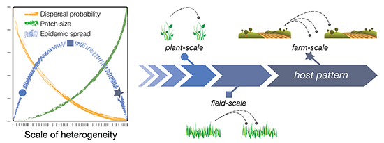
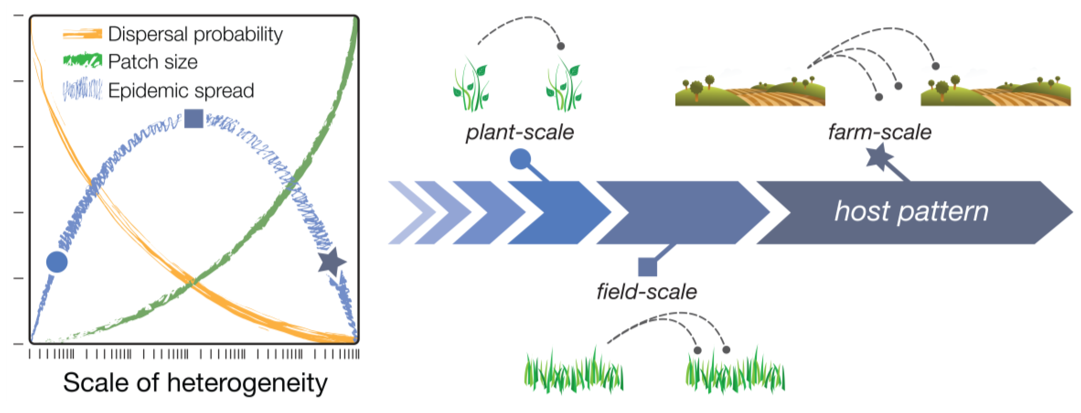
The dispersal scaling hypothesis (DSH) is a new theory in spatial ecology that formalizes the expected relationship between spatial heterogeneity, scale of heterogeneity, and pest or pathogen dispersal/epidemic spread. The DSH therefore provides a framework for quantifying inoculum interference, and its impact on epidemic outcomes. In formal terms: the DSH posits a unimodal (“humpbacked”) relationship between the magnitude of pest or pathogen infestation and the grain size (spatial resolution, or the finest scale of patchiness) of a host distribution [7,8]. In other words, the magnitude of dispersal (the number of pests or propagules moving from one patch to another) is predicted to increase with increasing grain size (scale) up to a certain point (the “hump”), after which the magnitude of dispersal declines (Figure 1; blue line). This is explained as follows. Initially, dispersal of infectious agents among host patches increases with patch size, as larger populations produce more dispersers and larger patches are more attractive or make bigger targets for dispersers (Figure 1; green line). Eventually, however, a maximum scale of patchiness is reached at which there are no further gains in dispersal, and the magnitude of dispersal instead begins to decline with further increases in grain size. This is because increasing the grain size (scale) of the landscape also increases the size of the gaps—the non-host areas—between patches, which has an overall depressive effect on dispersal (Figure 1; orange line). In summary, host patchiness can vary over a spectrum of scales (grain sizes), dispersal processes have a characteristic scale (the dispersal range of the pest or pathogen species), and the interplay between these different scales results in a unimodal distribution of dispersal magnitudes, and thus, pest or pathogen infestation. The exact grain size at which dispersal is maximized, however, depends on other aspects of spatial heterogeneity, such as the amount, quality, and distribution of habitat (or hosts) on the landscape [8].

The DSH has identified a potential for scale-dependent maxima in epidemic outcomes for a large variety of economically important pests and diseases under numerous different disease management scenarios and spatial configurations of host species, using a multi–model approach encompassing analytical and numerical techniques, deterministic and stochastic methods of dispersal, individual– and population–level movements, and multiple generations of spatiotemporal spread in complex landscapes [7,8]. As such, the DSH offers a credible new theoretical framework for quantifying the expected inoculum/disease pressure in heterogeneous host distributions at, e.g., plant-, plot-, field-, and landscape-scale. Thus, this sort of analysis could be of predictive value in optimizing the design of experiments to ensure that crop phenotypes are assessed in settings that simulate real agricultural (epidemic) situations. This will broaden their scope of inference to situations that more closely match commercial production settings, in terms of cultivar performance under realistic (natural) levels of inoculum/disease pressure. This is an obvious and desirable goal in the accurate quantification of complex plant phenotypes and selection of elite cultivars with relatively high QDR, or high yield in the presence of disease. In practice it may be the tool used to determine the best compromise or prioritization as pathogens with different and contrasting dispersal scales are frequently assessed together, thus giving a basis on which to determine whether assessments are likely to be over- or under-estimate estimates compared with real agricultural situations.

As originally written, the DSH formalized the expected relationship between the magnitude of a single generation of dispersal and the scale of host patchiness (i.e., spread from an infected area to a non-infected area), and the end result of many dispersal events and the scale of host patchiness (i.e., final epidemic extent in a landscape containing many host areas). In the current modelling study we investigated the influence of this scaling relationship on phenotyping of QDR. QDR is characterized by a reduced rate of epidemic development in a host crop variety attributed to various components of partial disease resistance, such as a lower infection frequency [11]. We therefore considered the temporal evolution of this scaling relationship (DSH) over the course of epidemics in crops with different resistance components. We also explored the influence of the wider environment in a number of scenarios that mimic varietal deployment in commercial production settings. Our objectives were to: (1) characterize the impact of the interaction of spatial heterogeneity and scale of heterogeneity on the progress of plant disease epidemics in crop varieties with varying levels of QDR; and (2) investigate this interaction as a potential confounding factor in the inference from ex-situ assessment of QDR to commercial production settings. As the generality of the theoretical predictions of the DSH have previously been demonstrated using a wide array of modelling assumptions [7,8], here we make a number of classic simplifying assumptions in theoretical epidemiology from which departures resulting from additional complexities can later be evaluated. We describe a simple, spatiotemporal model of the susceptible, exposed, infectious and removed (SEIR) type, which is the standard modelling approach in human disease epidemiology, and is also widely used in plant disease epidemiology, e.g., Skelsey et al. 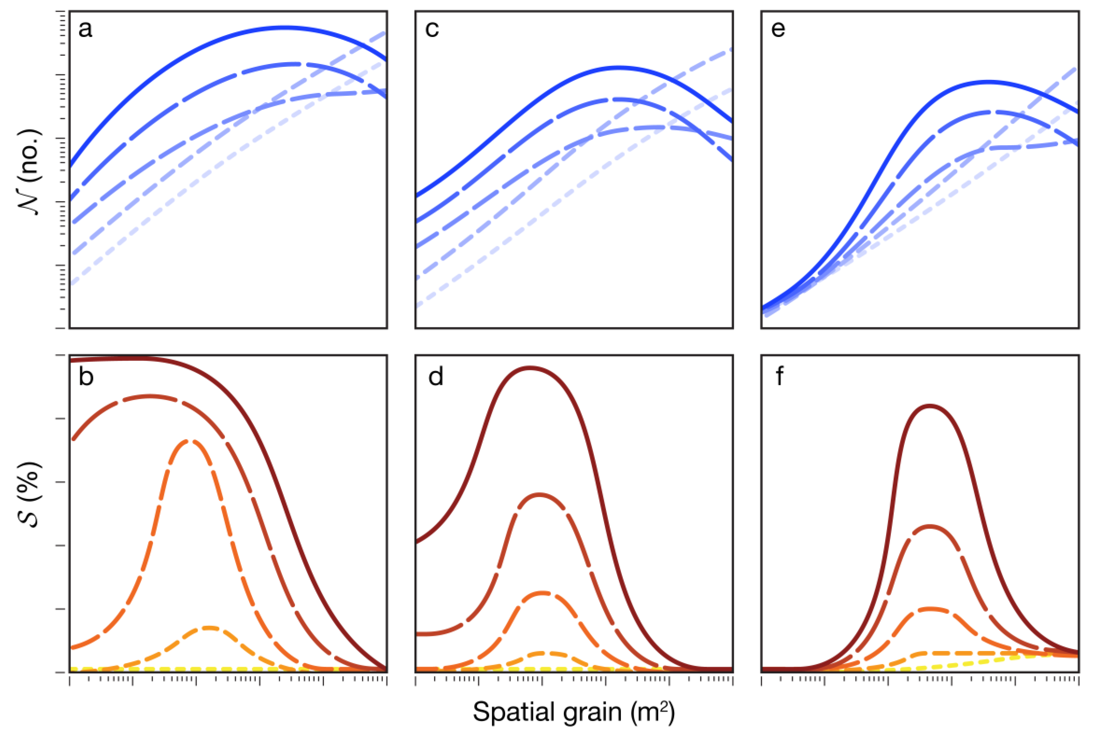[5,9]. In this approach, the host population is divided into several non-overlapping categories: healthy susceptible, latently infected, infectious, and removed (post-infectious). Space was simulated as a binary raster landscape (Cartesian grid) of host and non-host areas to create spatially heterogeneous landscapes in which various aspects of host pattern, such as host abundance and degree of aggregation, could be altered. The grain size (cell dimensions) of landscapes was varied to investigate the influence of the interaction of spatial heterogeneity and scale on epidemic progress. Grain size ranged over a spectrum of values from plant-, to plot-, to field-, to regional-level. Epidemic progress was characterized at regular intervals using the average number of successfully deposited spores (on healthy or infected tissue, whether within the same host patch or another host patch) per diseased patch, N (no.), and overall disease severity, S (%). 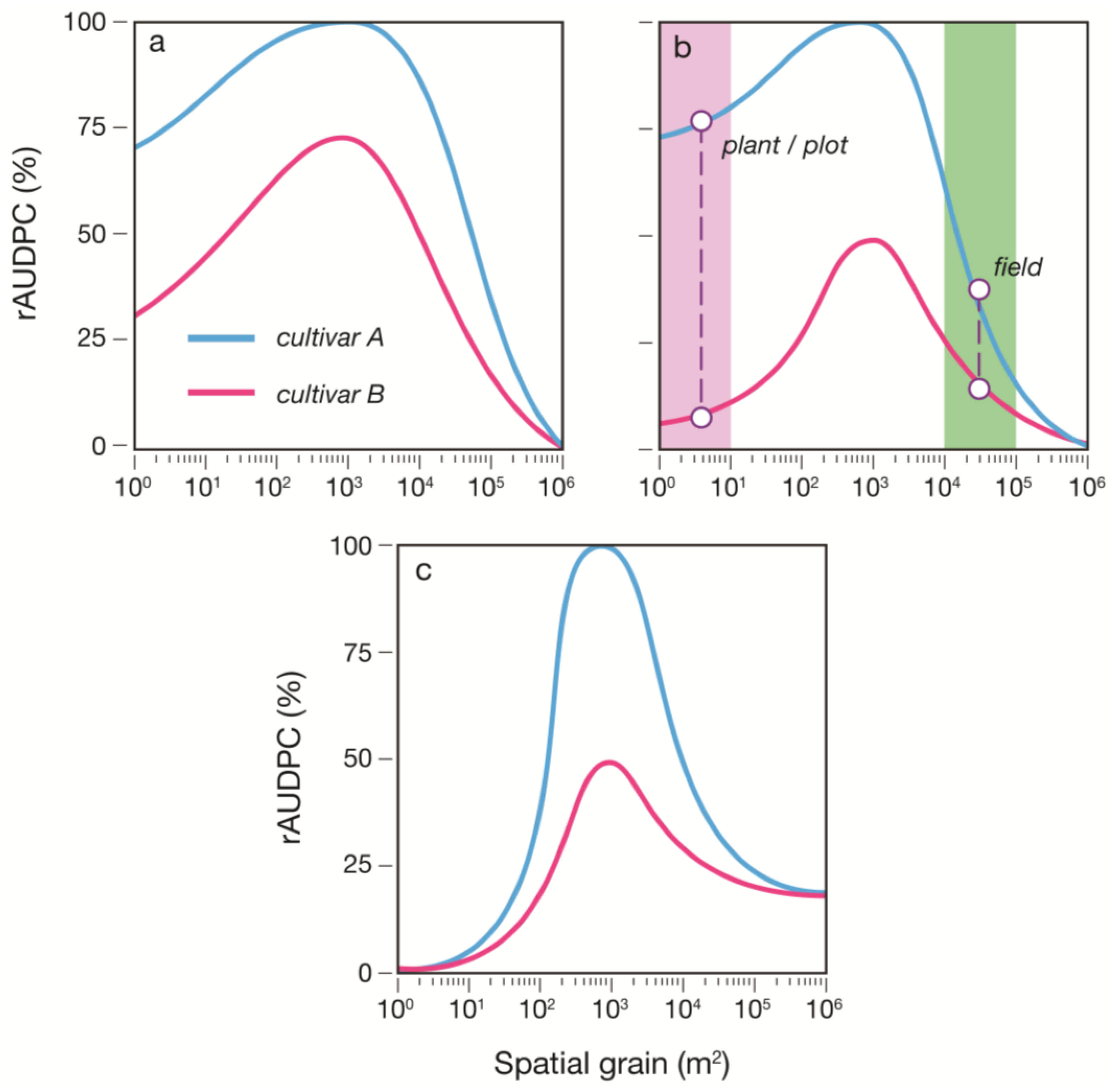At the end of each model run (epidemic), the area under the disease progress (S) curve (AUDPC; % days) was used to assess the impact of heterogeneity and scale on the relative difference in epidemic outcomes between varieties. Insights gained from this study and the recommendations made herein may inform the design of future phenotyping platforms to optimize the scale for QDR assessment.

Figure 1. Conceptual diagram of the dispersal scaling hypothesis (DSH). Scaling a heterogeneous host distribution relative to the gap–crossing abilities of a pest or pathogen produces a trade-off between the “benefits” (larger patches = more dispersers) and “costs” (dispersal distances become larger and harder to traverse) of increasing grain (patch) size. This results in a unimodal (“humpbacked”) relationship between dispersal or epidemic spread and scale of heterogeneity.

Figure 1. Conceptual diagram of the dispersal scaling hypothesis (DSH). Scaling a heterogeneous host distribution relative to the gap–crossing abilities of a pest or pathogen produces a trade-off between the “benefits” (larger patches = more dispersers) and “costs” (dispersal distances become larger and harder to traverse) of increasing grain (patch) size. This results in a unimodal (“humpbacked”) relationship between dispersal or epidemic spread and scale of heterogeneity.

2. Results and Discussion

2.1. Relationship between Heterogeneity, Scale, and Epidemic Progress

Contrary to previous predictions ([7,8]; Figure 1), the relationship between the magnitude of dispersal, N, and spatial grain (the finest scale of patchiness in the host distribution) was not unimodal (“humpbacked”) in the early stages of an epidemic in either clumped and abundant (Figure 2a), randomly distributed and abundant (Figure 2c), or randomly distributed and sparse (Figure 2e) host populations. This is explained as follows. During the initial stages of an epidemic the limiting factor for N is the number of infectious agents. The density of disease is low in infected areas and spore production is consequently minimal. The magnitude of N is therefore dictated by deposition of inoculum within the same host patch, as opposed to deposition in distant (other) host patches. In landscapes comprised of larger host patches with the same initial density of disease, the absolute amount of inoculum produced per infected patch is higher and more inoculum will deposit on host tissue within the same (larger) host patch. Thus, N increases monotonically with the scale of spatial heterogeneity in the initial stages of an epidemic.

During the latter stages of an epidemic the limiting factor for N is the distance between host patches. The proportion of healthy tissue decreases in infected areas and dispersal to distant host patches becomes increasingly important for multiplication of disease and increase in N. As the scale of landscape pattern increases, although the absolute amount of inoculum produced per (larger) infected patch is higher, the distance between host patches will ultimately increase too, eventually exceeding the gap-crossing abilities of the pest or pathogen. This decreases the probability of movement among patches, and the reduction in recruitment of new susceptible host patches has an overall depressive effect on N, leading to a unimodal relationship between spatial grain and N in the latter stages of an epidemic (Figure 2a,c,e). Model output therefore suggests that the relationship between N and scale of heterogeneity follows the DSH ([7,8]; Figure 1), provided that sufficient time has elapsed for the pathogen population to reach a density that promotes invasive spread (Figure 2; more solid lines).

As disease severity, S, accumulates over multiple generations of pathogen reproduction and spread, the unimodal relationship predicted by the DSH was apparent at earlier stages of an epidemic than for N. Consistent with previous predictions ([7,8]; Figure 2b,d,f), there was a unimodal relationship between S and spatial grain in all but the earliest interval of disease assessment.

Relative standard errors of N and S, when averaged across all spatial scales and landscape scenarios, were low at 0.3% and 3.3%, respectively. The level of replication was therefore deemed adequate for reducing noise in simulation outcomes to a level that did not obscure emergent patterns.

We explored a large parameter space with the model and found that the qualitative relationships for the impact of the interaction of heterogeneity and scale on epidemic progress closely matched those given in Figure 2. This lends weight to the generality of the theoretical predictions for the temporal evolution of the DSH. Nonetheless, we only say we expect these patterns to occur under the conditions tested (see Experimental section, and [7,8]), not that they will under every possible condition.

Figure 2. Magnitude of dispersal, N, and disease severity, S, for simulated epidemics in landscapes where the spatial grain (cell dimensions, m²) is systematically increased, under three landscape scenarios (across columns): (a,b) an aggregated and abundant host distribution; (c,d) a randomly distributed and abundant host distribution; and (e,f) a randomly distributed and sparse host distribution. The curves represent different stages (disease assessment intervals) of an epidemic, with dash size and colour intensity increasing with time after inoculation. It should be noted that the same qualitative relationships emerged under different parameterizations of the model, provided the axes and epidemic duration were scaled appropriately; we therefore do not provide values for N, and S.

Figure 2. Magnitude of dispersal, N, and disease severity, S, for simulated epidemics in landscapes where the spatial grain (cell dimensions, m²) is systematically increased, under three landscape scenarios (across columns): (a,b) an aggregated and abundant host distribution; (c,d) a randomly distributed and abundant host distribution; and (e,f) a randomly distributed and sparse host distribution. The curves represent different stages (disease assessment intervals) of an epidemic, with dash size and colour intensity increasing with time after inoculation. It should be noted that the same qualitative relationships emerged under different parameterizations of the model, provided the axes and epidemic duration were scaled appropriately; we therefore do not provide values for N, and S.

2.2. Relationship between Heterogeneity, Scale, and Relative Variety Performance

We next compared epidemics in two cultivars with different levels of QDR. The sensitivity of the model to the various components of QDR (θ, λ, ι, σ, ε) has previously been documented [5,12] and we selected infection efficiency, ε, as a suitable candidate parameter. We repeated the epidemic scenarios previously described using parameter values for a relatively resistant (ε = 0.01) and then a relatively susceptible variety (ε = 0.02). All other model parameters were identical and fixed at baseline values. This was a simplifying assumption from which departures resulting from additional complexities (e.g., variation in multiple components of QDR) can later be evaluated.

We summarized epidemics using the area under the disease progress curve (AUDPC; % days). This is commonly used in disease/yield loss studies and for quantitative resistance evaluation as it incorporates time of disease onset, rate of increasing intensity, and final intensity by integrating the area under the disease progress curve, S(t). To facilitate a comparison of the two crop varieties we calculated the relative AUDPC (rAUDPC; %) as a percentage of the peak AUDPC of the susceptible variety in each landscape scenario. rAUDPC values for the relatively susceptible (Figure 3; blue lines) and relatively resistant (Figure 3; pink lines) varieties were qualitatively very similar to the results for S for the final and penultimate intervals of disease assessment, respectively (Figure 2). This is expected as ε affects the rate of epidemic development and AUDPC is an integrated measure of epidemic progress. Notably, the difference in rAUDPC between the two cultivars was scale-dependent. This result seems counter-intuitive: if a pathogen realizes a lower infection frequency on one cultivar compared to another, then one might expect the factor difference in epidemic outcomes to remain constant in proportion to the factor difference in infection frequency. This is easily explained, however, using the DSH and the results from Figure 2: the variable scale of crop heterogeneity interacts with the characteristic scale of pathogen dispersal to produce scale-dependent differences in disease pressure, which compound over multiple generations of reproduction and spread. Notably, there was a large disparity between results at the plant-/plot- (e.g., 1 to 10 m²) and field-scale (e.g., 10⁴ m²) in all landscape scenarios. Consequently, varietal performance in designed experiments may be a poor guide to varietal performance in real agricultural settings. The various landscape scenarios we simulated here had the potential to modify the shape of this scaling relationship, but not the general unimodal form. When host crops were abundant, the difference in rAUDPC between varieties decreased with increasing scale (Figure 3a,b). When crop distributions were sparse, the difference in rAUDPC between varieties at first increased with scale up to a maximum corresponding with the peak level of disease, then decreased with increasing scale (Figure 3c). Thus, the difference between varieties was more pronounced at scales where the rate of epidemic spread (amongst crop areas) was high. Model results therefore suggest that the interaction of host heterogeneity and scale of heterogeneity is a determinant of varietal performance under epidemic conditions (Figure 3).

This is a previously unreported phenomenon that could have implications for future phenotyping trials aimed at selection of elite cultivars or lines with a high, relative, quantitative resistance to disease, or high yields in the presence of disease. As the results of this study demonstrate, accurate ranking of cultivars or lines according to their relative resistance to disease requires that the level of disease pressure of the designed experiment matches that of the crop in its commercial production setting. We recognize that limited space may necessitate assessment of QDR in pots or small unbordered plots, therefore we recommend some pragmatic approaches centred on manipulation of interplot (inoculum) interference to improve the inference from ex-situ assessment to commercial production settings. In the first instance, the DSH provides a number of simple analytical formulae that can be used to predict the impact of the interaction of host heterogeneity and scale on the magnitude of inoculum dispersal among experimental plants, and among commercial crops [7]. These formulae require only two epidemiological parameters to provide quantitative predictions: density of disease and a dispersal length scale. As such, the DSH is a tool that can provide hard and fast quantitative guidelines for experimental plot size and spacing to increase/reduce the level of negative and positive inoculum interference to better match commercial settings. Alternatively, the numerical modelling implementation of the DSH described here (a standard, spatially explicit SEIR model with a small number of parameters, applied over a spectrum of spatial scales of heterogeneity) can be used to predict the impact of the interaction of host heterogeneity and scale on spatiotemporal epidemic spread in experiments and commercial settings. Where adjustment of pot/plot size and spacing is insufficient to approximate epidemic conditions in commercial settings (as determined by the DSH), it may be possible to adjust initial inoculum doses, or control the rate of epidemic progress using agrochemicals or highly susceptible/infected host tissue (e.g., disease spreader rows), to reduce or increase disease pressure, respectively, as required.

Figure 3. Relative area under the disease progress curve (rAUDPC) for simulated epidemics in landscapes where the spatial grain (cell dimensions, m²) is systematically increased, under three landscape scenarios: (a) an aggregated and abundant host distribution; (b) a randomly distributed and abundant host distribution; and (c) a randomly distributed and sparse host distribution. The blue curve represents a relatively susceptible crop variety and the pink curve a relatively resistant variety, with an infection efficiency, ε (-), half the value of the former. Shaded areas delineate some characteristic domains of scale for phenotyping trials (purple) versus commercial production settings (green).

Figure 3. Relative area under the disease progress curve (rAUDPC) for simulated epidemics in landscapes where the spatial grain (cell dimensions, m²) is systematically increased, under three landscape scenarios: (a) an aggregated and abundant host distribution; (b) a randomly distributed and abundant host distribution; and (c) a randomly distributed and sparse host distribution. The blue curve represents a relatively susceptible crop variety and the pink curve a relatively resistant variety, with an infection efficiency, ε (-), half the value of the former. Shaded areas delineate some characteristic domains of scale for phenotyping trials (purple) versus commercial production settings (green).

3. Experimental Section

3.1. Plant Disease Epidemic (SEIR) Model

A spatially explicit, age-structured, integrodifference equation model was developed to simulate within- and between-patch dynamics of plant disease epidemics. The model is fully described elsewhere [9], therefore only the salient characteristics are described here. In addition to its coordinates, each cell was characterized by a single state variable describing the number of lesions in age classes of 1 day. All other variables were derived from this basic state variable. The equations describing the number of lesions for each cell were based on the following principles. Every day there was a new generation of lesions and these belonged to the same age class. Lesions were non-expanding and of a fixed area, θ (m²). Lesions were latent during the first λ days of their existence, the latency period. During each successive day, as another cohort of lesions reached age λ + 1, these lesions produced spores. Spore production intensity per unit of infectious leaf area was accounted for by the parameter σ (no. m⁻²). Infectiousness was taken to last ι days. When a cohort of lesions reached age λ + ι +1, they were classed as removed (necrotic) and no longer contributed to increase of disease. The age-structured population model for lesions in each host cell was updated daily, by “aging” the existing lesions by 1 day, and starting new lesions at a rate calculated as the product of: the number of landed spores per m² leaf area in a day, the infection efficiency, ε (-), and fraction of host area not yet occupied by disease. The areas of latent, infectious and dead lesion area in each host cell were calculated by multiplying the number of lesions in the appropriate age category with θ, and summing over all lesions. We did not model host growth or senescence, and the amount of leaf tissue per cell was characterized by the parameter γ (leaf area index; m² leaf/m² ground). Baseline parameterization was based on a previously published SEIR plant disease model [9], with: θ = 10⁻⁴, λ = 5, ι = 1, σ = 10⁶, ε = 10⁻², and γ = 5 (these are the host-pathogen interaction parameters, or components of quantitative disease resistance).

3.2. Inoculum Dispersal

We described where spores landed with a dispersal kernel, which describes the probability distribution (m⁻²) of landing locations of spores in the two-dimensional plane:

(1)

where α (m) is a distance parameter, and r (m) is the Euclidean distance between host cells. Dispersal kernels can differ strongly in shape, and theoretical studies suggest that the shape of the dispersal kernel, in particular the fatness of the tail, has a major effect on an organism’s potential to spread [13,14]. Equation 1 is called the square-root negative exponential kernel and is classed as a “fat-tailed” distribution (the decline of the tails is less than exponential). Kernels with fatter tails lead to expansion in “leaps and bounds” ahead of the expanding wave, which means accelerating expansion [14,15,16]. Ecologists interested in processes that operate at broad spatial scales, such as long-distance population spread, commonly employ fat-tailed kernels. The distance parameter, α, was set to 0.5 m, giving a mean spore dispersal distance of 10 m; the same order of magnitude as given previously in the literature [9].

3.3. Landscape Generation

We used fractal geometry to generate binary landscape patterns of host and non-host cells [17,18,19]. This method creates natural-looking landscape patterns and facilitates tight control over the degree of aggregation of host cells via a single parameter known as the Hurst exponent, H [20,21]. To fully evaluate interactions of host distribution, scale, and epidemic progress over time, we generated a series of 30 landscapes of increasing grain size (the specific cell dimensions); in other words, each landscape pattern was generated at 30 different grain sizes, spanning 1 to 10⁶ m². Landscapes were modelled as a 128 × 128-cell torus and were thus “wrapped” such that any spore dispersing outside of the borders of the grid “reappeared” on the opposite edge, equalizing immigration and emigration rates. This is a commonly used approach to approximate an infinite spatial extent [8,9,10,22,23,24,25,26]. Thus, whilst the grain size of landscapes varied across a range of 30 values, spatial extent was effectively infinite. Moreover, the fractal technique we used generates “periodic” landscape patterns that flow smoothly across borders when wrapped on a torus. This avoided dispersing spores experiencing sharp discontinuities in host distributions when they crossed from one edge of the landscape and reappeared on the other, further reducing edge effects.

3.4. Model Scenarios

3.4.1. Relationship between Heterogeneity, Scale, and Epidemic Progress

We implemented the model under three landscape scenarios: (i) abundant and aggregated host distribution, where the proportion of host in the landscape h = 0.25 and H = 1; (ii) abundant and random host distribution, where h = 0.25 and H = −0.5; and (iii) sparse and random host distribution, where h = 0.05 and H = −0.5. A total of 250 simulations were performed for each scenario. In each model run, a different fractal map was generated. Epidemics were initiated via a random sample, s, of 1% of host cells inoculated with n = 1 (latent) lesion per square metre. Perfect environmental conditions for disease were assumed, and epidemic progress was quantified at weekly intervals. Epidemics lasted 35 days as this was sufficient to reach full crop destruction in the most susceptible scenario. Epidemic progress was characterized using the following time- and space-dependent summary measures: (i) the average number of successfully deposited spores (whether within the same host patch or another host patch) per diseased patch, N (no.); and (ii) overall disease severity, S (%), expressed as the percentage of host tissue in the landscape that is either latently infected, infectious or necrotic. Values of N and S were averaged over model iterations within each landscape scenario. To investigate if model results for the interaction of heterogeneity, scale, and epidemic progress were qualitatively similar across a large parameter space, we repeated the above set of simulation experiments, independently increasing/decreasing each model parameter value (θ, λ, ι, σ, ε, γ, α, s, n) in turn by a factor of two, (whilst holding other parameters constant).

3.4.2. Relationship between Heterogeneity, Scale, and Relative Variety Performance

We repeated the epidemic scenarios previously described using parameter values for a relatively resistant (ε = 0.01) and then a relatively susceptible variety (ε = 0.02). All other parameters were fixed at their baseline values. Based on the daily overall disease severity, S, the area under disease progress curve (AUDPC; % days) was calculated for each host variety, as described by Campbell and Madden [27]. To compare variety performance under the different landscape scenarios, AUDPCs were normalized to relative AUDPCs (rAUDPC; %), where rAUDPC is the percentage of the AUDPC of the susceptible variety under each landscape scenario.

3.5. Statistical Analyses

Relative standard errors of N and S (standard error expressed as a percentage of the mean) were calculated between iterations for each landscape scenario, in order to assess the level to which the precision of simulation results were affected by variability in the random maps, and the number of repetitions performed. We examined underlying trends over time and space for each summary measure with smoothed-line plots. Line smoothing was done with a cubic spline routine in the MATLAB numerical computing environment.

4. Conclusions

This study refines and extends new ecological theory (the DSH) by characterising the relationship between host heterogeneity, scale of heterogeneity, and the progress of plant disease epidemics in crop varieties with varying levels of QDR. We conclude that this relationship follows the DSH, with the proviso that sufficient time has elapsed to promote invasive spread. We further conclude that the interaction between host heterogeneity and scale is an important determinant of varietal performance (in terms of relative resistance to disease) under epidemic conditions. We advise that accurate ranking of cultivars or lines according to their relative resistance to disease requires that the level of disease pressure of the designed experiment matches that of the crop in its commercial production setting as closely as possible. To achieve this, we recommend that interplot (inoculum) interference is considered as an experimental variable that could be manipulated to ensure conformity in the level of disease pressure between experiment and deployment. The degree of manipulation required can be determined with minimal knowledge of the pathosystem of interest using the quantitative framework of the DSH. Pot/plot size and spacing, initial inoculum dose, and rate of epidemic progress (using agrochemicals, or a continuous supply of inoculum) can then be adjusted within the parameters defined by the DSH.

Plot trialling designs are always a compromise between costs, equipment constraints, seed quantity and many other operational factors. They are also required to produce data for many and sometimes conflicting purposes. Add to this the conflicting scale demands for assessing the effects of different diseases simultaneously, and the scope for change is often limited. Similarly, the costs and practicality of inoculation are often prohibitive. Use of agrochemicals to control inoculum can introduce pleiotrophic confounding factors. However, even where changes cannot be made, or even where further compromises have to be made for cost or other practical reasons, the DSH provides the rationale and parameterisation for adjusting relative pathogen performance to that likely to be expressed under farm-scale conditions.

References

1. Munns, R.; James, R.A.; Xu, B.; Athman, A.; Jordans, C.; Conn, S.J.; Byrt, C.S.; Hare, R.A.; Tyerman, S.D.; Tester, M.; et al. Grain yield of modern wheat on saline soils is improved by ancestral hkt gene. Nat. Biotechnol. 2012, 30, 360–364. [Google Scholar] [CrossRef]
2. Passioura, J.B. The perils of pot experiments. Funct. Plant Biol. 2006, 33, 1075–1079. [Google Scholar] [CrossRef]
3. Rebetzke, G.J.; Fischer, R.T.A.; van Herwaarden, A.F.; Bonnett, D.G.; Chenu, K.; Rattey, A.R.; Fettell, N.A. Plot size matters: Interference from intergenotypic competition in plant phenotyping studies. Funct. Plant Biol. 2013, 41, 107–118. [Google Scholar]
4. Paysour, R.E.; Fry, W.E. Interplot interference: A model for planning field experiments with aerially disseminated pathogens. Phytopathology 1982, 73, 1014–1020. [Google Scholar] [CrossRef]
5. Skelsey, P. Multi-Scale Modeling of Potato Late Blight Epidemics; Wageningen Universiteit: Wageningen, The Netherlands, 2008; p. 257. [Google Scholar]
6. Vanderplank, J.E. Plant Diseases: Epidemics and Control; Academic Press: New York, NY, USA, 1963; p. 349. [Google Scholar]
7. Skelsey, P.; With, K.; Garrett, K. Why dispersal should be maximized at intermediate scales of heterogeneity. Theor. Ecol. 2013, 6, 203–211. [Google Scholar] [CrossRef]
8. Skelsey, P.; With, K.A.; Garrett, K.A. Pest and disease management: Why we shouldn’t go against the grain. PLoS One 2013, 8, e75892. [Google Scholar] [CrossRef]
9. Skelsey, P.; Rossing, W.A.H.; Kessel, G.J.T.; Powell, J.; van der Werf, W. Influence of host diversity on development of epidemics: An evaluation and elaboration of mixture theory. Phytopathology 2005, 95, 328–338. [Google Scholar] [CrossRef]
10. Skelsey, P.; Rossing, W.A.H.; Kessel, G.J.T.; van der Werf, W. Invasion of Phytophthora infestans at the landscape level: How do spatial scale and weather modulate the consequences of spatial heterogeneity in host resistance? Phytopathology 2010, 100, 1146–1161. [Google Scholar] [CrossRef]
11. Zadoks, J.C.; Schein, R.D. Epidemiology and Plant Disease Management; Oxford University Press: New York, NY, USA, 1979; p. 427. [Google Scholar]
12. Skelsey, P.; Kessel, G.J.T.; Rossing, W.A.H.; van der Werf, W. Parameterization and evaluation of a spatiotemporal model of the potato late blight pathosystem. Phytopathology 2009, 99, 290–300. [Google Scholar] [CrossRef]
13. Clark, J.S. Why trees migrate so fast: Confronting theory with dispersal biology and the paleorecord. Am. Nat. 1998, 152, 204–224. [Google Scholar]
14. Kot, M.; Lewis, M.A.; van den Driessche, P. Dispersal data and the spread of invading organisms. Ecology 1996, 77, 2027–2042. [Google Scholar] [CrossRef]
15. Mollison, D. Spatial contact models for ecological and epidemic spread. J. R. Stat. Soc. B 1977, 39, 283–326. [Google Scholar]
16. Shaw, M.W. Simulation of population expansion and spatial pattern when individual dispersal distributions do not decline exponentially with distance. Proc. R. Soc. London B 1995, 259, 243–248. [Google Scholar] [CrossRef]
17. Keitt, T.H. Spectral representation of neutral landscapes. Landsc. Ecol. 2000, 15, 479–493. [Google Scholar] [CrossRef]
18. Mandelbrot, B.B. The Fractal Geometry of Nature; W.H. Freeman and Co: New York, NY, USA, 1982; p. 495. [Google Scholar]
19. Voss, R.F. Random fractal forgeries. In Fundamental Algorithms for Computer Graphics; Earnshaw, R.A., Ed.; Springer-Verlag: Berlin, Germany, 1985; pp. 805–835. [Google Scholar]
20. With, K.A.; Gardner, R.H.; Turner, M.G. Landscape connectivity and population distributions in heterogeneous environments. Oikos 1997, 78, 151–169. [Google Scholar] [CrossRef]
21. With, K.A.; King, A.W. The use and misuse of neutral landscape models in ecology. Oikos 1997, 79, 219–229. [Google Scholar] [CrossRef]
22. Haase, P. Spatial pattern analysis in ecology based on Ripley’s K-function: Introduction and methods of edge correction. J. Veg. Sci. 1995, 6, 575–582. [Google Scholar] [CrossRef]
23. Hastings, A.; Gross, L.J. Encyclopedia of Theoretical Ecology; University of California Press: Berkeley, NC, USA, 2012; p. 848. [Google Scholar]
24. Kuuluvainen, T.; Rouvinen, S. Post-fire understory regeneration in boreal Pinus sylvestris forests with different fire histories. J. Veg. Sci. 2000, 11, 801–812. [Google Scholar] [CrossRef]
25. Peterson, C.J.; Squiers, E.R. An unexpected change in spatial pattern across 10 years in an aspen-white pine forest. J. Ecol. 1995, 83, 847–855. [Google Scholar] [CrossRef]
26. Skelsey, P.; Van Der Werf, W.; Kessel, G.J.T.; Rossing, W.A.H.; Holtslag, A.A.M. Multi-scale modelling of infection pressure from Phytophthora infestans. EPPO Bull. 2007, 37, 313–316. [Google Scholar] [CrossRef]
27. Campbell, C.L.; Madden, L.V. Introduction to Plant Disease Epidemiology; Wiley-Interscience: New York, NY, USA, 1990; p. 532. [Google Scholar]