Spatial Relation of Apparent Soil Electrical Conductivity with Crop Yields and Soil Properties at Different Topographic Positions in a Small Agricultural Watershed

Abstract

Use of electromagnetic induction (EMI) sensors along with geospatial modeling provide a better opportunity for understanding spatial distribution of soil properties and crop yields on a landscape level and to map site-specific management zones. The first objective of this research was to evaluate the relationship of crop yields, soil properties and apparent electrical conductivity (ECa) at different topographic positions (shoulder, backslope, and deposition slope). The second objective was to examine whether the correlation of ECa with soil properties and crop yields on a watershed scale can be improved by considering topography in modeling ECa and soil properties compared to a whole field scale with no topographic separation. This study was conducted in two headwater agricultural watersheds in southern Illinois, USA. The experimental design consisted of three basins per watershed and each basin was divided into three topographic positions (shoulder, backslope and deposition) using the Slope Position Classification model in ESRI ArcMap. A combine harvester equipped with a GPS-based recording system was used for yield monitoring and mapping from 2012 to 2015. Soil samples were taken at depths from 0–15 cm and 15–30 cm from 54 locations in the two watersheds in fall 2015 and analyzed for physical and chemical properties. The ECa was measured using EMI device, EM38-MK2, which provides four dipole readings ECa-H-0.5, ECa-H-1, ECa-V-0.5, and ECa-V-1. Soybean and corn yields at depositional position were 38% and 62% lower than the shoulder position in 2014 and 2015, respectively. Soil pH, total carbon (TC), total nitrogen (TN), Mehlich-3 Phosphorus (P), Bray-1 P and ECa at depositional positions were significantly higher compared to shoulder positions. Corn and soybeans yields were weakly to moderately (<±0.75) correlated with ECa. At the deposition position at the 0–15 cm depth ECa-H-0.5 was weakly correlated (r < ±0.50) with soil pH and was moderately correlated (r = ±0.50–±0.75) with organic matter (OM), calcium (Ca) and sulfur (S). Slope variation from 1%–20% at the research site had a strong influence on soil properties at watershed scale. When data from all topographic positions were combined together in all basins spatial interpolation between Mehlich-3 P and ECa-H-0.5 resulted in a larger cross validation RMSE compared to individual shoulder and backslope positions. Results demonstrated that topographic position should be considered while making correlations of ECa with soil properties. Methods of delineating topography positions presented in this paper can easily be replicated on other fields with similar landscape characteristics and EMI sensor based survey techniques can certainly improve and help in making detailed prediction maps of soil properties.

1. Introduction

Geophysical methods such as electromagnetic induction (EMI) can be used to study the spatial variability of soil physical, chemical, and hydrological properties at the field to the small catchment scales [1,2,3,4,5,6]. The EMI technique can measure apparent soil electrical conductivity (ECa) by inducing an electrical current in the soil [7]. This method provides a relatively accurate, non-invasive, fast and inexpensive measurement of ECa [8,9,10]. Traditional soil sampling and EMI techniques together can provide better understanding of spatial variability in soils [1,11]. The ECa is influenced by soil properties such as salinity, temperature, water content and bulk density [12]. Brevik et al. [7] conducted a study on soils with different water content and found that ECa changes temporally and is highly dependent on soil moisture. Many studies have shown correlation of ECa with soil properties important for plant growth and crop yields including soil compaction, depth of claypan, soil water content, soil texture, drainage, TC, TN, soluble salts, extractable P and soil pH [3,12,13,14]. Drier and coarser soils are less electrically conductive than wetter and finer soils [15]. Bronson et al. [16] concluded that ECa can be used as potential tool to provide information about soil properties such as clay content and extractable Ca in the U.S. Southern High Plains, but that spatial covariance needs to be considered as it can improve estimation of ECa. Changes in bulk density resulting from management practices within or between fields on the order of 0.12 to 0.13 g·cm⁻³ lead to changes in soil ECa affecting soil interpretations made in the field using the EM-38 [17]. Previous studies on ECa relationship with soil properties and crop yields either on small field scale or watershed scale, were carried out without considering the effects of topographic positions (such as shoulder, backslope, and deposition slope). Kitchen et al. [4] investigated the three contrasting soil-crop systems for relationship of ECa and topographic measures (elevation, slope, curvature and aspect) to crop yields. They found that ECa alone better explained the yield variability compared to topographic variables. Temporal and spatial variation in crop yields is affected by many factors such as climate, soil properties, management practices and topographic position of the field [18]. A complete knowledge of factors and their interactions that affect yield is required for site specific yield management [19].

Crop yields can be highly related to topography as it causes changes in physical and chemical properties of upslope and downslope soils that includes soil nutrients, OM, redistribution of soil particles and water availability due to both vertical and horizontal water redistribution [19,20]. The ridge tops or upper slope surfaces can experience intense solar radiation and high wind velocity resulting in dry conditions and high erosion and soil movement [21]. Lower slope positions are subjected to soil OM and moisture accumulation. Characteristics of mid-slope positions vary in between the upper and lower slope positions. A study conducted on two corn-soybean fields showed that combined effects of topography and soil varied annually and were responsible for 30%–85% of variability in observed yields in seven site-years out of nine studied [18]. Many studies have reported correlations of topography with soil properties including soil water content, soil carbon, temperature and microclimate conditions [22,23,24,25,26,27]. A study by Florinsky et al. [28] showed that the topography influence on soil properties and residual phosphorus decreased with depth. However, the influence of topography on crop yields has been reported over relatively small scales [29,30].

Topographic influence on crop yields intensifies at watershed scales due to higher variability in soil properties, precipitation, temperature and other climatic factors [19]. There is limited information on ECa correlations with soil properties and crop yields at different topographic positions at the watershed scale. To better understand the relation of ECa with soil properties and crop yields, it is important to compare the ECa correlations with soil properties and crop yields at different topographic positions as well as the whole field without delineating topographic position. It is also important to determine for better site-specific management whether the correlation of ECa with soil properties can be improved by adding topographic position as compared to whole field scale modeling. Therefore, the first objective of this research was to study the changes in soil properties, crop yield and ECa and their correlations at different topographic positions (shoulder, backslope, and deposition) at our present study site with relatively significant differences in slope varying from 1%–20%. The second objective was to examine whether the correlation of ECa with soil properties and crop yields on a watershed scale can be improved by considering topography compared to the whole field scale (no topographic separation) in modeling ECa and soil properties.

2. Materials and Methods

2.1. Study Site and Experimental Design

This study was conducted on two headwater agricultural watershed areas adjacent to Southern Illinois University Carbondale’s Tree Improvement Center (TIC) (Lat. 37°42′34″ N, Long. 89°16′08″ W) located on west side of Carbondale, IL, USA (Figure 1). Two watersheds were delineated in ESRI ArcMap (version 10.2.2) using the hydrology toolbox with a digital elevation model (DEM raster resolution of 1.219 × 1.219 m) generated from LIDAR data available on geospatial database for state of Illinois [31]. Areas of watershed 1 and 2 were 9.83 and 26.10 ha, respectively. The dominant soil series at the study site was classified as Hosmer silt loam (Fine-silty, mixed, active, mesic Oxyaquic Fragiudalfs). The Hosmer series is a moderately well drained soil that formed from loess found on hill sides and with slopes ranging from 1%–20%. The watersheds contain a perched, seasonal water table at a depth of 0.46 to 0.76 m, varying with the time of year (Soil Survey Staff, 2015). This site has been managed in a corn-soybean crop rotation under no-tillage [32]. Soybean was planted on 3 June and 10 June in 2012 and 2014, respectively. Soybean was harvested on 9 October and 22 October in 2012 and 2014, respectively. Corn was planted on 10 May and harvested on 10 November in 2013. In 2015, corn was planted on 3 May and harvested on 1 October. Weather data including average monthly air temperature, total monthly precipitation and total monthly potential evapotranspiration (PET) was obtained from nearest weather station were provided by Water and Atmospheric Resources Monitoring Program, Illinois Climate Network (2015), Figure 2.

Experimental design consists of three basins per watershed (Basin 1, 2, 3 in watershed 1 and basin 4, 5, 6 in watershed 2) (Figure 1). Each basin was delineated in ESRI ArcMap (Version 10.2.2) using a DEM (raster resolution 1.219 × 1.219 m) and hydrology toolbox. Each basin was further divided into three topographic positions (shoulder, backslope and deposition). These delineated topographic positions (shoulder, backslope and deposition) were used to assess the influence of topography on soil properties, yield and ECa (measured using EM38-MK2). The model used for delineating topographic positions is a direct adaption of the Slope Position Classification model by Evans et al. [33] who modified the Topographic Position Index (TPI) tool created by Jenness [34]. The Slope Position Classification model developed by Evans et al. [33] delineates four topographic positions (e.g., flat, deposition, backslope and shoulder) instead of six topographic positions (valley, lower slope, middle slope, upper slope, ridge, and flat areas) defined by Jenness [34]. The TPI is the difference of a cell elevation (e) in a DEM from the mean elevation (μe) of a user specified area surrounding e:

TPI = e – μe

(1)

• If TPI ≈ 0, the cell is either on a flat plane or on a plane with nearly equal slope, e.g., a backslope.
• If TPI > 0, the cell is on a convex plane or shoulder slope.
• If TPI < 0, the cell is on a concave plane or deposition slope.

A radius of 125 m was used to determine the TPI in each watershed individually and a TPI raster was outputted from the DEM. A larger radius of 125 m was chosen so that microscale topographic variation within each plot could be omitted.

2.2. Data Collection

Soil samples were taken from 54 locations (6 basins × 3 topographic positions per basin × 3 sampling locations per topographic position) over the study area including both watersheds in 2015 (Figure 1). Three soil or yield sampling locations were assigned randomly to each topographic position in every basin and composite samples of 10 soil cores were collected from each of these assigned sampling locations in a radius of 3 m. Soil samples were collected using stainless steel push probes at depth increments of 0–15 cm and 15–30 cm in October, 2015 after harvesting of corn. All soil samples were air-dried and grounded to pass through a sieve with 2 mm openings. The soil samples were analyzed by Brookside Laboratories for standard soil fertility parameters (such as pH, OM, TC, TN, Bray-1 P, Mehlich-3 P, and Mehlich-3 extractable elements) using standard soil testing procedure. Details of soil tests performed are given in Brookside Laboratories [35]. Texture analysis of soil samples was done using hydrometer method [36].

Corn and soybeans were harvested with combine harvesters and yields were measured by the yield monitors installed in the combine harvesters. Yield measurements were taken by grain sensors, with each measurement covering an area of about 2 by 6 m (2 m is an average forward distance traveled by a combine during 1 s, and 6 m is the width of the combine header). Simultaneously, site coordinates were determined by a GPS unit. The moisture content for corn and soybean grain yields was adjusted to 15% and 13%, respectively.

Apparent soil electrical conductivity was measured using an electromagnetic induction device EM38-MK2 (Geonics Limited) on transects separated at 5 m on the study area. A wooden trailer made without any metal joints was used for carrying EM38-MK2 for ECa survey. The ECa measurement were taken in October 2015 and soil moisture content varied from 21% to 23% at the time of ECa measurements. Raw ECa data obtained from EM38-MK2 were offset by 1.5 s to compensate for the positional accuracy of the GPS antenna ahead of the sensor and for time lags in the data acquisition system [9]. The EM38-MK2 is constructed by mechanically and electrically integrating two standard EM38-MK2 ground conductivity meters. For horizontal dipole (ECa-H) measurements, the bottom instrument’s transmitter-receiver dipoles are oriented parallel to the earth surface and for the vertical dipole (ECa-V) measurements, top instrument’s transmitter-receiver dipoles are oriented perpendicular to the earth surface. In the ECa-V mode, the primary magnetic field can effectively penetrate to a depth of 1.5 m and 0.75 m, while the ECa-H mode is effective for shallower investigation (0.75 m and 0.45 m). Two modes of operation ECa-H and ECa-V provided four dipole readings ECa-H-0.5 (effective depth of electromagnetic field penetration = 0.45 m), ECa-H-1 (effective depth of electromagnetic field penetration = 0.75 m), ECa-V-0.5 (effective depth of electromagnetic field penetration = 0.75 m), and ECa-V-1 (effective depth of electromagnetic field penetration = 1.5 m). Details of equipment, its operation, accuracy, and uses are discussed by Corwin and Lesch [37].

2.3. Statistical and Spatial Analysis

Cluster and outlier analysis (Anselin Local Moran’s I) was performed on ECa and yield data and outliers (high low and low high) from data were removed in ESRI ArcGIS 10.3.1. The ECa and yield data were measured close to the soil sampling locations used for the soil properties. The ECa and yield data were collocated using ordinary kriging in ArcMap to produce the ECa and yield data at the 54 soil sampling locations. Ordinary kriging is an accepted method for obtaining collocated data [38]. For evaluating the effect of topographic positions on variables (soil properties, crop yield and ECa), a nested mixed model using Proc Glimmix was developed in SAS 9.4 (SAS Institute). Two way interaction of topography and depth with all variables were analyzed using Tukey-Kramer grouping and least squares means were calculated at alpha = 0.05. In brief, the topographic positions are nested under basins, and the basins are nested under two watersheds. Basin was a nested, random factor as not all basins within the watershed were sampled (Figure 1 and Figure 3). Pearson Correlation Coefficients between soil properties, crop yield and ECa were also calculated using Proc Corr in SAS 9.4 (SAS Institute).

Following an explanatory data analysis, Mehlich-3 P at 0–15 cm soil depth and ECa-H-0.5, Mehlich-3 Na at 15–30 cm and ECa-V-1 were selected to develop simple cokriging models [39]. Before developing cokriging models, trend analysis and semivariogram/covariance cloud in geostatistical analysis toolset of ESRI ArcGIS 10.3.1 were analyzed for above variables. Experimental variograms were computed and modelled to describe the spatial variation in Mehlich-3 P, Mehlich-3 Na and ECa. If the shape of the experimental variogram suggested that regional trend was present in the variation, low-order polynomials (first, second and third) were fitted on the co-ordinates. A separate simple cokriging model was developed on whole basin scale without any topographic separation and this model was compared with three separate models at three topographic positions. Cross-validation root mean square error (RMSE) along with details of models are shown in Section 3.7.

3. Results and Discussion

3.1. Climatic Condition during Different Growing Season

Total annual precipitation during growing season was in the following order: 2015 (147.24 cm) > 2014 (111.07 cm) > 2013 (101.80 cm) > 2012 (68.55 cm). The 20-year average annual total precipitation was 113.49 cm (Figure 2). Year 2015 was the wettest as the total annual precipitation was higher than the 20-year average annual precipitation. In the Unites States, the year 2012 was considered as one of the worst drought years in the past 80 years or more, causing yields reductions of crops such as winter wheat, corn, and soybean [40,41]. The total monthly precipitation at the time of soybean planting during the June month in 2012 was 9.3 and 8.9 cm less compared to 2014 and 20-years average monthly precipitation. However, the monthly precipitation during the June month in 2014 was not significantly lower than 20-year average monthly precipitation. In 2014, the average monthly precipitation in month of April and May was 7.5 and 3.7 cm higher compared to 20-year average monthly precipitation. Total monthly precipitation in May at the time of corn planting in 2013 and 2015 was lower than the 20-year average monthly precipitation. However, the monthly precipitation in months after corn planting was higher in 2015 compared to 2013. In 2013, the monthly precipitation during the first three months after corn planting were similar providing more consistent soil moisture conditions for plant growth. In 2015, the precipitation in June was 11.13 and 10.18 cm higher compared to monthly precipitation in 2013 and 20-year average monthly precipitation. The higher soil moisture conditions in 2015 than 2013 after corn planting might have interfered with plant growth. The air temperatures during June in 2012 and 2014 at the time of soybean planting showed no big differences (Figure 2). In July, the air temperature was higher in 2012 than in 2014. The air temperatures in the month of May showed only small differences in 2013 and 2015.

3.2. Influence of Topographic Position on Corn and Soybean Yields

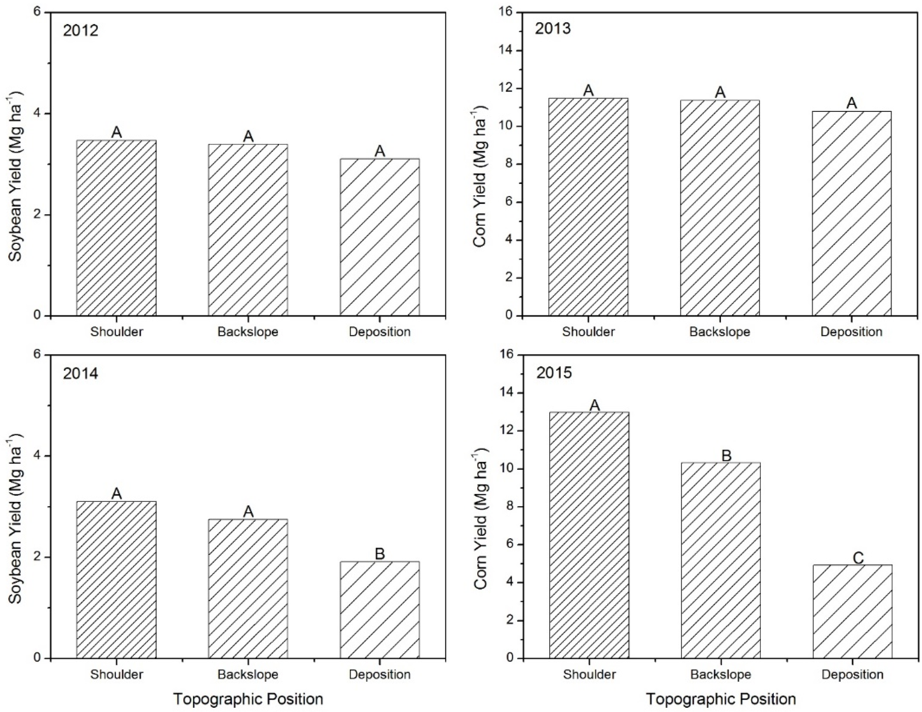
There were no significant differences in soybean and corn yields among the three topographic positions in 2012 and 2013. The mean soybean and corn grain yields averaged over all topographic position in 2012 and 2013 were 3.32 and 11.21 Mg·ha⁻¹ (Figure 4). In 2014, the soybean grain yield from depositional topographic position was significantly less than shoulder and backslope positions. Soybean yields from the depositional position was 38% lower from than yields from the shoulder position. The mean soybean yields averaged over all topographic positions was 2.59 Mg·ha⁻¹ in 2014. 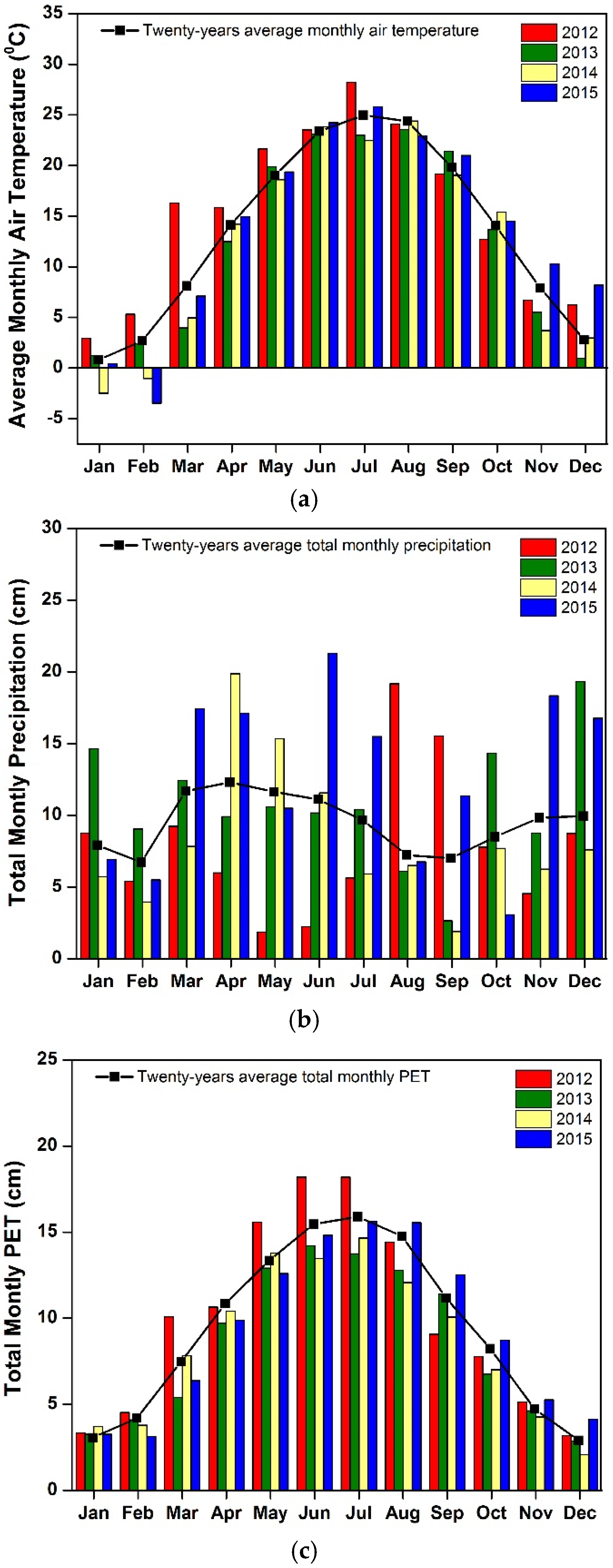Soybeans yields were lower in 2014 growing season than 2012 (Figure 4). In 2015, corn grain yields were significantly different at all three topographic positions. Corn grain yields at the deposition position were 62% and 52% lower than yields at shoulder and backslope positions, respectively. The backslope position resulted in 20% lower corn grain yields compared to the shoulder position in 2015. The annual variability in crop yields can be attributed to weather differences among years. Drier soil conditions resulting from lower precipitation during 2012 might have caused drought stress on soybeans causing lower yields overall, irrespective of topographic positions. The year 2015 was the wettest year compared to other years and may have resulted in different yields at all three topographic positions. Higher precipitation in April and May in 2014 (before soybean planting) as well as during May and June in 2015 resulted in excessive soil moisture conditions which may have caused waterlogging at the deposition position. The anaerobic soil conditions caused by the waterlogged soils resulted in poor plant stand establishment and growth and consequently, lowering grain yields in 2014 and 2015. Soybean is more sensitive to excessive soil moisture conditions compared to corn [42]. Crop yields were significantly different at topographic position in years with total annual precipitation equal or higher than 20-year average annual precipitation. Dry years showed no differences at various topographic positions. Many studies have shown yearly differences in crop yields due to topography [18,19,43,44,45,46]. In agreement with our results, Muñoz et al. [44] also reported that topography had major influence on corn yields during the year with higher precipitation. A study conducted by Halvorson and Doll [29] in eastern Oregon, Washington and North Dakota showed that landscape position and slope aspect significantly influences the grain yield of wheat. Jones et al. [47] reported that corn, sorghum and soybean yields were also affected by landscape positions and slope length. Thelemann et al. [48] observed that higher water retention for longer periods of time resulted in lower corn grain and stover yields at depositional and flat areas, whereas well drained summit positions had the highest yields as these slope positions drained earlier. Depression areas can accumulate water in turn they can impact corn and soybean yields and significant difference in yield can be observed during wet and dry years of precipitation in these areas [46]. Depth to B horizon can play an important role in regulating yields at different topographic positions. Khakural et al. [45] reported decreased yields of corn and soybean at backslope position compared to foot and upper toe slopes and concluded that it was due to eroded backslope positions. Based on the observed differences in rainfall patterns over 4 years, it is speculated that soil saturation in the early spring may be an important factor affecting differences in N availability to corn and soybean plants among the different landscape positions.

3.3. Influence of Topographic Position on ECa

ECa-H-1, ECa-V-1 and ECa-V-0.5 were significantly lower at shoulder positions compared to backslope and deposition positions (Figure 5). ECa-H-0.5 showed significant differences at all three topographic positions, with the lowest value at shoulder position and highest values at deposition position. Topographic influence on ECa can be attributed to clay and soil moisture content at time of data collection. In a no-till corn/soybean fields low ECa values were observed at higher elevation compared to high ECa values at low elevation [49]. Brevik et al. [7] concluded that ECa may increase with an increase in volumetric water content due to strong relation (r² = 0.70) between them. They also observed that higher elevation soil sampling locations had lower ECa values compared to lower elevations due to higher volumetric water content at lower elevation positions. Hanna et al. [50] observed soil moisture content during crop growth period using neutron probes and reported that within slope positions, soils on the foot slopes and backslopes contained on an average of 4 cm more available water than soils on the summits and shoulder slopes. Differences observed in soil moisture content may contribute towards variation in ECa values at different topographic position.

3.4. Influence of Topographic Position on Soil Properties

Sand content at depth 15–30 cm for shoulder position was significantly lower compared to deposition position (

Table 1. Changes in soil properties due to topographic positions at different depths.

	Topographic Position
	Shoulder		Backslope		Deposition
Depth (cm)	0–15	15–30	0–15	15–30	0–15	15–30
Sand, g·kg−1	126.27 ab †	95.81 b	124.12 ab	100.36 ab	122.25 ab	132.25 a
Silt, g·kg−1	630.74 ab	618.38 abc	593.89 bc	580.90 c	652.10 a	640.02 a
Clay, g·kg−1	242.99 cd	285.81 ab	281.99 bc	318.74 a	225.65 d	227.73 d
pH	6.411 ab	5.928 b	6.144 ab	5.894 b	6.433 ab	6.850 a
TEC, meq/100 g	12.969 c	15.637 abc	18.298 ab	20.845 a	14.859 bc	13.183 bc
OM, %	1.988 a	0.823 b	2.073 a	0.809 b	2.098 a	1.138 b
TN, %	0.106 a	0.048 c	0.107 a	0.044 c	0.108 a	0.072 b
TC, %	1.064 a	0.386 c	1.084 a	0.381 c	1.133 a	0.707 b
P ‡ mg·kg−1	41.444 ab	18.333 cd	28.167 bc	9.222 d	63.278 a	27.667 cbd
Bray-1 P, mg·kg−1	45.889 ab	15.500 c	26.667 bc	4.944 c	64.667 a	27.111 bc
Ca ‡ mg·kg−1	1843.440 ab	1670.941 b	2256.561 a	1962.728 ab	1936.671 ab	1737.064 b
Mg ‡ mg·kg−1	135.670 c	176.222 bc	292.722 ab	419.56 a	261.065 bc	286.111 abc
K ‡ mg·kg−1	157.780 a	89.778 cd	152.610 a	103.280 bc	126.170 ab	66.056 d
Na ‡ mg·kg−1	25.833 c	34.389 bc	45.167 bc	92.722 ab	92.000 b	134.390 a
S ‡ mg·kg−1	9.111 c	14.278 c	9.833 c	18.278 c	28.222 a	36.278 a
Fe ‡ mg·kg−1	149.720 cd	125.834 d	173.446 bc	130.561 d	278.561 a	196.941 b
Al ‡ mg·kg−1	689.780 bc	894.781 a	751.564 b	941.835 a	599.285 c	626.332 c
Mn ‡ mg·kg−1	159.670 a	70.611 bc	89.944 b	36.000 c	139.786 a	159.226 a
B ‡ mg·kg−1	0.591 ab	0.457a b	0.569 ab	0.442 b	0.669 a	0.649 ab
Cu ‡ mg·kg−1	1.747 ab	1.280 b	1.639 ab	1.184 b	2.276 a	2.154 a

^† Means followed by the same letter within a row do not differ significantly at p < 0.05 according to Tukey-Kramer grouping test; ^‡ Mehlich-3 extractable elements; Abbreviations: TEC, Total Exchange Capacity; OM, Organic matter; TN, Total Nitrogen; TC, Total Carbon; P, Phosphorus; Mg, Magnesium; K, Potassium; Na, Sodium; S, Sulfur; Fe, Iron; Al, Aluminum; Mn, Manganese; Cu, Copper.

). Mean silt content at the deposition position was higher than shoulder and significantly higher than at the backslope position for both depths (Table 1). Mean clay content at depth 15–30 cm for the backslope position (31.874%) was greatest compared to other topographic positions. This could be due to higher percent slope change and more eroded top layer at the backslope position. The deposition position had significantly lower clay content at both depths compared to backslope and shoulder position (Table 1). At a depth of 15–30 cm, soil pH at the deposition position was significantly higher than the shoulder and backslope positions. However, no significant differences were obtained for soil pH for individual topographic positions between two depths. Total exchanges capacity was highest at the shoulder position at depth 15–30 cm compared to 0–15 cm depth at the shoulder and deposition positions as well as at 15–30 cm depth at the deposition position. At all topographic positions, OM, TN and TC were significantly lower at depth 15–30 cm compared to depth 0–15 cm. At 15–30 cm the deposition position had higher TN and TC than the shoulder and backslope position. Mehlich-3 P and Bray-1 P were significantly higher at 0–15 cm depth at the deposition position compared to other positions except at shoulder position from 0–15 cm depth. Significantly lower P concentrations were evident at the 15–30 cm depth at the backslope position. Physical removal of surface soil from steep slopes may decrease the concentration of N at shoulder position; however, it can rejuvenate the supply of rock derived nutrients such as P at shoulder positions [51]. At 15–30 cm depth, the shoulder and deposition position had similar Ca concentrations, which were significantly lower from Ca concentrations at backslope position from depth 0–15 cm. The Mg concentration at shoulder position from upper soil layer was significantly lower compared to backslope position Mg concentrations at both depths. Highest Mg concentration was obtained at backslope position from depth 15–30 cm, which was not significantly different to Mg concentration at 0–15 cm depth. The K concentrations were relatively higher at surface layers for all three topographic positions. Lowest K concentration was at 15–30 cm depth from deposition position, which was not significantly different from K concentrations from same depth at the shoulder position. The highest concentration of Na was obtained at the deposition position from depth 15–30 cm which was significantly higher than Na concentrations at 0–15 cm depth from all topographic positions and from 15–30 cm depth from the shoulder position. The S concentrations were significantly higher at the deposition position than both the shoulder and backslope positions for both depths. Concentration of Fe was significantly higher at the deposition position than the shoulder and backslope position for 15–30 cm depth. The highest Fe concentration was obtained within the surface layer of deposition position. The Al concentrations were significantly higher at the lower depth (15–30 cm) for all three topographic positions (Table 1). Backslope positions have significantly lower Mn concentrations at both depths compared to other two topographic positions. The B concentration showed no significant differences at all positions except at the backslope positon from depth 15–30 cm and at the deposition position at 0–15 cm depth. Surface layers have higher Cu concentrations compare to lower depth 15–30 cm. A study conducted by Wei et al. [52] found that deposition of eroded soil from upper positions into lower positions of landscape resulted in increase in TC, TN, silt and clay content from upper slope to foot slope along slope position gradients. An increase in soil organic carbon and total P from shoulder slope towards the toe slope in upper 25 cm depth of soil profile was observed by Heckrath et al. [53]. Yimer et al. [54] also reported significant differences in soil properties such as soil texture, soil pH, plant available phosphorus, CEC, exchangeable base cations, and percent base saturations. The differences were attributed to topographic aspect-induced microclimatic differences resulting in leaching and OM content differences within soil profile. Slope and aspect can determine the level and location of run-off and infiltration, which can influence the variation in water content and deposition of salts. Salts, pH, Na and CEC levels were observed to be greater in low elevation area when compared to high elevation areas [49].

3.5. Correlation of ECa with Crop Grain Yields at Three Topographic Positions

In 2013, corn grain yields were moderately correlated (r = ±0.50–±0.75) to ECa-H-0.5 at the shoulder position, and with ECa-H-1, ECa-V-0.5 and ECa-V-1 at the deposition (

Table 2. Correlation between ECa dipoles and soybean and corn grain yields.

Topographic Position	Crop	Year	Apparent Electrical Conductivity
			ECa-H-0.5	ECa-H-1	ECa-V-0.5	ECa-V-1
Shoulder	Soybean	2012	−0.208	0.060	0.397	0.230
		2014	0.278	−0.273	0.019	−0.372
	Corn	2013	0.606 *	0.066	0.072	0.168
		2015	0.105	0.138	0.001	0.122
Backslope	Soybean	2012	−0.410	−0.378	−0.324	−0.250
		2014	−0.058	−0.286	−0.411	−0.331
	Corn	2013	−0.390	−0.331	−0.307	−0.251
		2015	0.121	−0.097	−0.136	−0.088
Deposition	Soybean	2012	−0.284	−0.249	−0.106	−0.211
		2014	0.218	0.038	0.184	0.124
	Corn	2013	−0.374	−0.514 *	−0.506 *	−0.504 *
		2015	−0.002	−0.263	−0.030	0.053
All Basins ††	Soybean	2012	−0.276 *	−0.265 *	−0.141	−0.204
		2014	−0.381 *	−0.489 *	−0.449 *	−0.494 *
	Corn	2013	−0.118	−0.291	−0.252	−0.252
		2015	−0.464 *	−0.522 *	−0.479 *	−0.475 *

* Significant at 0.05 probability level; ^†† All basins combined with no topographic separation.

). Soybean grain yields showed no significant correlation with ECa at different topographic positions. However, soybean yields are weakly correlated (r < ±0.50) with ECa-H-0.5 and ECa-H-1 in 2012 and 2014 in all basins, when data are combined over all topographic positions. Soybean yields were also weakly correlated (r < ±0.50) with ECa-V-0.5 and ECa-V-1 in 2014. For the year 2015, both corn grain yields were weakly correlated (r < ±0.50) with ECa, when data was combined over all topographic positions. Kitchen et al. [4] concluded that ECa alone can explain corn and soybean yield variability (averaged over sites and years R² = 0.21) better than topographic variables (averaged over sites and years R² = 0.17). Two out of three research sites monitored for yield had weak correlations (r < ±0.50) with ECa averaged over three years [4]. Higher average annual precipitation during year 2015 (147.24 cm) and 2014 (111.07 cm) compared to 2013 (101.80 cm) and 2012 (68.55 cm) may have played an important role in contributing to soil moisture levels in 2015 and 2014, thus resulting in better correlations of ECa to yield. Kitchen et al. [5] concluded that precipitation received during the growing season for corn and soybeans may play an important role in governing ECa correlation to grain yields.

3.6. Correlation of ECa with Soil Properties at Three Topographic Positions

A moderate correlation (r = ±0.50–±0.75) was observed between ECa-H-0.5 and elevation with all basins without topographic separation (

Table 3. Correlation coefficient between soil properties and ECa-H-0.5.

Properties	Depth (cm)	Apparent ECa-H-0.5
		Shoulder n = 18	Backslope n = 18	Deposition n = 18	All Basins †† n = 54
Elevation, m		−0.376	0.137	0.143	−0.647 *
Slope, %		0.447	0.075	−0.098	0.093
Aspect, degree		0.578	−0.409	−0.295	−0.362 *
Sand, g·kg−1	0–15	−0.409	0.242	0.256	−0.017
	15–30	0.654 *	0.298	−0.271	0.333 *
Silt, g·kg−1	0–15	0.063	−0.353	−0.285	−0.066
	15–30	−0.159	−0.507 *	0.492 *	−0.015
Clay, g·kg−1	0–15	0.266	0.123	0.071	0.079
	15–30	−0.336	0.358	−0.216	−0.208
pH (1:1 H2O)	0–15	0.140	−0.096	0.482 *	0.060
	15–30	0.374	0.015	0.419	0.396 *
TEC, meq/100 g	0–15	0.396	0.359	0.190	0.448 *
	15–30	0.179	0.349	−0.463 *	0.092
OM, %	0–15	0.029	−0.198	0.533 *	0.121
	15–30	0.120	−0.448	0.227	0.215
TN, %	0–15	−0.153	−0.277	0.180	−0.045
	15–30	0.069	−0.564 *	0.143	0.199
TC, %	0–15	−0.238	−0.287	0.255	0.022
	15–30	0.082	−0.558 *	0.171	0.262 *
P ‡, mg·kg−1	0–15	0.670 *	-0.360	0.355	0.296 *
	15–30	0.806 *	0.214	0.234	0.273 *
Bray-1 P, mg·kg−1	0–15	0.580 *	−0.383	0.328	0.228
	15–30	0.763 *	0.122	0.244	0.285 *
Ca ‡, mg·kg−1	0–15	0.274	0.095	0.500 *	0.292 *
	15–30	0.736 *	0.246	−0.287	0.292 *
Mg ‡, mg·kg−1	0–15	0.456 *	0.477 *	0.338	0.616 *
	15–30	0.446 *	0.690 *	0.066	0.519 *
K ‡, mg·kg−1	0–15	−0.354	0.128	0.351	−0.245
	15–30	0.205	0.408	0.039	−0.020
Na ‡, mg·kg−1	0–15	0.253	0.393	0.131	0.532*
	15–30	0.206	0.473 *	−0.088	0.536 *
S ‡, mg·kg−1	0–15	0.006	0.000	0.500 *	0.459 *
	15–30	−0.590 *	0.255	0.442	0.360 *
Fe ‡, mg·kg−1	0–15	0.794 *	−0.158	0.013	0.511 *
	15–30	0.600 *	0.294	−0.064	0.509 *
Al ‡, mg·kg−1	0–15	−0.121	0.399	−0.269	−0.121
	15–30	−0.331	−0.019	−0.470 *	−0.423 *
Mn ‡, mg·kg−1	0–15	0.231	−0.046	0.114	−0.143
	15–30	0.366	0.066	0.103	0.358 *
B ‡, mg·kg−1	0–15	0.337	−0.059	0.180	0.194
	15–30	0.397	0.065	0.211	0.350 *
Cu ‡, mg·kg−1	0–15	0.482 *	−0.119	0.348	0.371 *
	15–30	0.528 *	0.091	0.277	0.490 *

^†† All basins combined with no topographic separation; Abbreviations: TEC, Total Exchange Capacity; OM, Organic matter; TN, Total Nitrogen; TC, Total Carbon; P, Phosphorus; Mg, Magnesium; K, Potassium; Na, Sodium; S, Sulfur; Fe, Iron; Al, Aluminum; Mn, Manganese; Cu, Copper; ^‡ Mehlich-3 extractable elements; * Significant at 0.05 probability level.

). However, no significant correlation was observed between ECa-H-0.5 and percent slope for all basins, and a weak correlation (r < ±0.50) was observed between ECa-H-0.5 and percent slope at the shoulder position. Correlation between ECa-H-0.5 and aspect at the shoulder position was moderate (r = ±0.50–±0.75) and for all basins with no topographic separation was weak (r < ±0.50). ECa-H-0.5 at 15–30 cm depth had a moderate (r = ±0.50–±0.75) correlation with sand at the shoulder position and weak correlation (r < ±0.50) with sand with all basins combined with no topographic separation. Weak and moderate correlation was observed between ECa-H-0.5 and silt at the backslope and deposition at 15–30 cm (Table 3). ECa-H-0.5 was weakly correlated (r < ±0.50) with soil pH from depth 0–15 cm and TEC from depth 15–30 cm, respectively at the deposition position. Combining the data for all topographic positions resulted in weak correlation (r < ±0.50) of ECa-H-0.5 with soil pH at 15–30 cm depth as well as with TEC at depth 0–15 cm. ECa-H-0.5 was moderately correlated (r = ±0.50–±0.75) with OM, Ca and S at the depositional position for depth 0–15 cm. ECa-H-0.5 showed weak negative correlation with Al at the deposition position at a depth of 15–30 cm. The negative correlation of Al increased, whereas the positive correlation of Ca and S decreased with ECa-H-0.5 when data were combined over all topographic positions. At the backslope position, TN, TC and Mg showed moderate correlation (r = ±0.50–±0.75) with ECa-H-0.5 for depth 15–30 cm. Total N and TC was negatively correlated with ECa-H-0.5 at this depth. Mg showed positive and weak correlation for depth 0–15 cm, which improved to moderate correlation (r = ±0.50–±0.75) if analyzed in absence of any topographic positions. When data were analyzed by removing the topographic positions, the correlations of Na was improved and resulted in moderate correlation (r = ±0.50–±0.75) with ECa-H-0.5. Mehlich-3 P and Bray-1 P showed a moderate (r = ±0.50–±0.75) and a moderate to strong correlation (r > ±0.75) with ECa-H-0.5 for 0–15 cm and 15–30 cm soil depth at the shoulder position, respectively. However, the correlations decreased to weak (r < ±0.50) when Mehlich-3 P and Bray-1 P were analyzed by combining data over topographic positions. At the shoulder position only, Fe, Ca and Cu showed a significant positive correlation with ECa-H-0.5. The correlation of ECa-H-0.5 with Fe and Cu decreases when data were combined for all topographic positions. The correlation of S at shoulder position with ECa-H-0.5 reversed when data were combined over all topographic positions.

The significant positive correlations of ECa-H-1 was obtained for elevation at the deposition position and the following soil properties: soil pH at deposition positions; clay at the shoulder position for depth 0–15 cm; TEC at the shoulder positions for both depths; Mehlich-3 P, Bray-1 P, and Cu at the shoulder position for both depths; Mg at all three topographic positions for both depths; Na at the backslope position for both depths; S at the deposition position for both depths; K and Fe at depth 15–30 cm and Ca at depth 0–15 cm for the shoulder position; Ca and Na at depth 15–30 cm and K at depth 0–15 cm for deposition positions (

Table 4. Correlation coefficient between soil properties and ECa-H-1.

Properties	Depth (cm)	Apparent ECa-H-1
		Shoulder n = 18	Backslope n = 18	Deposition n = 18	All Basins †† n = 54
Elevation, m		0.038	0.122	0.368 *	−0.568 *
Slope, %		0.394	0.034	−0.234	0.086
Aspect, degree		0.075	−0.100	0.036	−0.327 *
Sand, g·kg−1	0–15	−0.405	0.189	0.210	0.016
	15–30	0.142	0.257	−0.376	0.144
Silt, g·kg−1	0–15	−0.284	−0.538 *	−0.260	−0.215
	15-30	−0.433	−0.012	0.142	−0.020
Clay, g·kg−1	0–15	0.575 *	0.334	0.089	0.206
	15–30	0.377	−0.111	0.296	−0.078
pH (1:1 H2O)	0–15	0.429	0.053	0.347	0.107
	15–30	0.043	0.411	0.474 *	0.403 *
TEC, meq/100 g	0-15	0.544 *	0.209	0.224	0.475 *
	15–30	0.470 *	−0.113	−0.235	0.060
OM, %	0–15	0.307	0.053	0.021	0.168
	15–30	−0.105	−0.434	−0.165	0.088
TN, %	0–15	−0.271	−0.135	0.029	−0.042
	15–30	−0.264	−0.305	−0.127	0.114
TC, %	0–15	−0.295	−0.097	0.011	0.025
	15–30	−0.267	−0.286	−0.100	0.189
P ‡, mg·kg−1	0–15	0.570 *	0.040	0.024	0.177
	15–30	0.484 *	−0.166	−0.155	0.029
Bray-1 P, mg·kg−1	0–15	0.573 *	0.086	−0.034	0.122
	15–30	0.458 *	−0.155	−0.182	0.044
Ca ‡, mg·kg−1	0–15	0.614 *	0.024	0.060	0.304 *
	15-30	0.386	0.031	−0.494 *	0.144
Mg ‡, mg·kg−1	0-15	0.592 *	0.536 *	0.610 *	0.708 *
	15–30	0.588 *	0.595 *	0.471 *	0.595*
K ‡, mg·kg−1	0–15	0.077	0.065	0.510 *	−0.101
	15–30	0.580 *	−0.112	−0.113	−0.056
Na ‡, mg kg−1	0–15	0.052	0.568 *	0.549	0.640 *
	15–30	0.347	0.665 *	0.488 *	0.707 *
S ‡, mg·kg−1	0–15	0.031	0.296	0.501 *	0.463 *
	15–30	0.230	0.268	0.492 *	0.460 *
Fe ‡, mg·kg−1	0–15	0.440	−0.042	−0.043	0.436 *
	15–30	0.523 *	−0.004	−0.262	0.331 *
Al ‡, mg·kg−1	0–15	−0.127	0.084	0.046	−0.095
	15–30	0.148	−0.383	−0.218	−0.348 *
Mn ‡, mg·kg−1	0–15	−0.121	−0.302	−0.094	−0.344 *
	15–30	0.000	0.352	−0.261	0.195
B ‡, mg·kg−1	0–15	0.323	0.076	0.121	0.176
	15–30	−0.105	0.201	0.074	0.221
Cu‡, mg·kg−1	0–15	0.500 *	0.232	−0.060	0.278 *
	15–30	0.537 *	−0.068	0.113	0.373 *

^†† All basins combined with no topographic separation; Abbreviations: TEC, Total Exchange Capacity; OM, Organic matter; TN, Total Nitrogen; TC, Total Carbon; P, Phosphorus; Mg, Magnesium; K, Potassium; Na, Sodium; S, Sulfur; Fe, Iron; Al, Aluminum; Mn, Manganese; Cu, Copper; ^‡ Mehlich-3 extractable elements; * Significant at 0.05 probability level.

). The correlation of ECa-H-1 decreased for all ions except Mg and Na. No significant correlation was obtained for Mehlich-3 P and Bray-1 P when data were combined over all topographic positions. Al at 0–15 cm and Fe and Mn at depth 15–30 only showed weak correlations (r < ±0.50) with ECa-H-1 when data were combined over topographic positions.

The significant and positive correlations of ECa-V-0.5 was obtained for following soil properties: soil pH at all three topographic positions; Mehlich-3 P, Bray-1 P, Ca, Fe and Cu at the shoulder position for both depths; B at the shoulder position at depth 0–15 cm (r > ±75); Mg at backslope and deposition positions for both depths; Al, Mn and soil pH at depth 15–30 cm for backslope positions; Na at the backslope position; Ca, Na and Fe at the deposition positions at 15–30 cm (

Table 5. Correlation coefficient between soil properties and ECa-V-0.5.

Properties	Depth (cm)	Apparent ECa-V-0.5
		Shoulder n = 18	Backslope n = 18	Deposition n = 18	All Basins †† n = 54
Elevation, m		−0.028	0.158	0.551 *	−0.506 *
Slope, %		0.319	−0.009	0.013	0.074
Aspect, degree		0.267	−0.148	−0.060	−0.291 *
Sand, g·kg−1	0–15	−0.119	0.073	0.539 *	0.103
	15–30	0.289	0.225	−0.365	0.195
Silt, g·kg−1	0–15	−0.129	−0.483 *	−0.419	−0.186
	15–30	−0.362	0.099	0.047	0.005
Clay, g·kg−1	0–15	0.210	0.378	−0.055	0.113
	15–30	0.181	−0.206	0.388	−0.134
pH (1:1 H2O)	0–15	0.601 *	−0.001	0.450 *	0.196
	15–30	0.338	0.488 *	0.504 *	0.501 *
TEC, meq/100 g	0–15	0.422	0.250	−0.096	0.399 *
	15–30	0.240	−0.157	−0.060	0.000
OM, %	0–15	0.266	0.007	−0.062	0.136
	15–30	−0.141	−0.423	−0.324	0.042
TN, %	0–15	−0.188	−0.094	−0.077	−0.061
	15–30	−0.177	−0.307	−0.068	0.124
TC, %	0–15	−0.243	−0.078	−0.121	−0.015
	15–30	−0.189	−0.287	−0.042	0.188
P ‡, mg·kg−1	0–15	0.724 *	0.060	−0.018	0.241
	15–30	0.573 *	−0.125	−0.183	0.081
Bray-1 P, mg·kg−1	0–15	0.782 *	0.093	−0.061	0.214
	15–30	0.580 *	−0.100	−0.208	0.106
Ca ‡, mg·kg−1	0–15	0.655 *	0.041	−0.090	0.302 *
	15–30	0.469 *	0.082	−0.497 *	0.167
Mg ‡, mg·kg−1	0–15	0.376	0.532 *	0.459 *	0.624 *
	15–30	0.329	0.582 *	0.568 *	0.542 *
K ‡, mg·kg−1	0–15	0.049	0.056	0.440	−0.116
	15–30	0.327	−0.141	0.010	−0.097
Na ‡, mg·kg−1	0–15	0.357	0.660 *	0.372	0.605 *
	15–30	0.062	0.747 *	0.573 *	0.723 *
S ‡, mg·kg−1	0–15	0.239	0.247	0.287	0.384 *
	15–30	−0.053	0.300	0.414	0.399 *
Fe ‡, mg kg−1	0–15	0.491 *	−0.048	−0.268	0.398 *
	15–30	0.461	−0.010	−0.541 *	0.304 *
Al ‡, mg kg−1	0–15	−0.299	0.093	0.141	−0.139
	15–30	−0.145	−0.506 *	0.130	−0.409 *
Mn ‡, mg·kg−1	0–15	0.346	−0.215	−0.103	−0.164
	15–30	0.146	0.532 *	−0.159	0.285 *
B ‡, mg·kg−1	0–15	0.770 *	−0.035	0.030	0.264 *
	15–30	0.212	0.230	0.166	0.316 *
Cu ‡, mg·kg−1	0–15	0.821 *	0.283	−0.100	0.425 *
	15–30	0.580 *	0.004	−0.104	0.391 *

^†† All basins combined with no topographic separation; Abbreviations: TEC, Total Exchange Capacity; OM, Organic matter; TN, Total Nitrogen; TC, Total Carbon; P, Phosphorus; Mg, Magnesium; K, Potassium; Na, Sodium; S, Sulfur; Fe, Iron; Al, Aluminum; Mn, Manganese; Cu, Copper; ^‡ Mehlich-3 extractable elements; * Significant at 0.05 probability level.

). Correlations with ECa-V-0.5 decreased for Cu, Mn, Fe, Na and Ca, when data were combined over topographic positions. Correlation improved for Mg at depth 0.15 cm. Correlation of ECa-V-0.5 with TEC and S were only obtained when data was combined over topographic positions.

The soil properties that showed significant correlations with ECa-V-1 were sand at the deposition position at 0–15 cm deep (r = ±0.50–±0.75); silt at backslope and deposition for 0–15 cm depth (r < ±0.50); clay at the shoulder position at 0–015 cm (r = ±0.50–±0.75); TEC, Mehlich-3 P, Bray-1 P, and Cu at shoulder positions for both depths; Mg at all three topographic positions; Fe and K from depth 15–30 cm and Ca at depth 0–15 cm at the shoulder position; Soil pH at depth 15–30 cm for backslope and deposition positions; Al and Mn at the backslope position from depth 15–30 cm; Na at the backslope position; Ca and Fe at the deposition position from depth 15–30 cm (

Table 6. Correlation coefficient between soil properties and ECa-V-1.

Properties	Depth (cm)	Apparent ECa-V-1
		Shoulder n = 18	Backslope n = 18	Deposition n = 18	All Basins †† n = 54
Elevation, m		−0.089	0.191	0.562 *	−0.540 *
Slope, %		0.392	−0.075	−0.075	0.028
Aspect, degree		−0.020	−0.150	−0.058	−0.368 *
Sand, g·kg−1	0–15	−0.228	0.099	0.539 *	0.132
	15–30	0.074	0.197	−0.319	0.147
Silt, g·kg−1	0–15	−0.423	−0.491 *	−0.490 *	−0.244
	15–30	−0.337	0.100	0.116	0.058
Clay, g·kg−1	0–15	0.561 *	0.364	0.025	0.151
	15–30	0.322	−0.194	0.256	−0.150
pH (1:1 H2O)	0–15	0.446	0.021	0.371	0.112
	15–30	0.010	0.493 *	0.507 *	0.455 *
TEC, meq/100 g	0–15	0.550 *	0.182	−0.143	0.373 *
	15–30	0.460 *	−0.165	−0.207	−0.006
OM, %	0–15	0.407	0.014	0.064	0.163
	15–30	0.063	−0.436	−0.257	0.099
TN, %	0–15	−0.229	−0.074	0.030	−0.014
	15–30	−0.143	−0.272	−0.125	0.151
TC, %	0–15	−0.241	−0.047	−0.014	0.048
	15–30	−0.158	−0.260	−0.083	0.223
P ‡, mg·kg−1	0–15	0.60 *	0.041	0.030	0.192
	15–30	0.440 *	−0.149	−0.071	0.064
Bray-1 P, mg·kg−1	0–15	0.611 *	0.076	0.006	0.145
	15–30	0.492 *	−0.127	−0.091	0.089
Ca ‡, mg·kg−1	0–15	0.682 *	0.026	−0.062	0.246
	15–30	0.287	0.102	−0.475 *	0.131
Mg ‡, mg·kg−1	0–15	0.550 *	0.468 *	0.316 *	0.608 *
	15–30	0.494 *	0.559 *	0.456 *	0.538 *
K ‡, mg·kg−1	0–15	0.126	0.043	0.403	−0.123
	15–30	0.454 *	−0.129	0.057	−0.116
Na ‡, mg·kg−1	0–15	0.009	0.610 *	0.209	0.582 *
	15–30	0.274	0.723 *	0.440	0.732 *
S ‡, mg·kg−1	0–15	0.001	0.228	0.167	0.379 *
	15–30	0.315	0.260	0.305	0.420 *
Fe ‡, mg·kg−1	0–15	0.415	−0.082	−0.329	0.377 *
	15–30	0.493 *	−0.022	−0.570 *	0.263 *
Al ‡, mg·kg−1	0–15	0.000	0.091	0.133	−0.086
	15–30	0.105	−0.470 *	0.077	−0.380 *
Mn ‡, mg·kg−1	0–15	−0.059	−0.185	−0.121	−0.281 *
	15–30	0.121	0.533 *	−0.097	0.287 *
B ‡, mg·kg−1	0–15	0.310	−0.010	−0.085	0.105
	15–30	−0.047	0.258	0.074	0.265 *
Cu ‡, mg·kg−1	0–15	0.556 *	0.262	−0.071	0.286 *
	15–30	0.645 *	0.001	−0.133	0.356 *

^†† All basins combined with no topographic separation; Abbreviations: TEC, Total Exchange Capacity; OM, Organic matter; TN, Total Nitrogen; TC, Total Carbon; P, Phosphorus; Mg, Magnesium; K, Potassium; Na, Sodium; S, Sulfur; Fe, Iron; Al, Aluminum; Mn, Manganese; Cu, Copper; ^‡ Mehlich-3 extractable elements; * Significant at 0.05 probability level.

). The correlations with ECa-V-1 improved only for Al, Fe at the deposition position and Mg at the shoulder and deposition position when data was combined over topographic positions.

Topographic and landscape properties including elevation, slope, curvature and aspect were weakly correlated (r < ±0.50) to ECa (shallow and deep) for three different soil textures [4]. Elevation was negatively correlated to ECa when all basins were combine together and our results were in agreement with results observed by Peralta and Costa [49]. Results from a multi-state dataset collected by Sudduth et al. [6] on ECa and soil properties showed weak to moderate correlations of ECa with clay content and CEC across most fields. Correlations of ECa with other soil properties including soil moisture, silt, sand, organic C and paste EC were lower and more variable for the fields across North-central USA [6]. A positive correlation between ECa and clay content was observed at four of six sites in southern high plains of Texas [16]. Clay content was not significantly correlated to ECa except for ECa-H-1 and ECa-V-1 at 0–15 cm depth on shoulder position at our research site. In another study, conducted by Carroll and Oliver [13] moderate and moderate to strong correlation were observed between ECa and soil textural fractions (sand, silt and clay) at two separate research sites. The relations between ECa and the topsoil properties were stronger than those for the subsoil. A negative correlation was observed for sand and bulk density with ECa as large bulk densities were associated with sandy soil [13]. Heil and Schmidhalter [55] investigated spatial distribution of clay, silt, and sand/gravel on highly variable landscape in Germany and concluded that clay and sand/gravel were most closely related to the ECa, and observed R² values ranging between 0.67 and 0.76. Jung et al. [3] observed a significant positive correlation of ECa with clay content at 15–30 cm depth and a negative correlation with silt and a weak correlation of ECa with sand.

Many studies reported a correlation between cation exchange capacity and ECa, which can be attributed to clay content in a soil profile [3,6,16]. No significant results were observed in our research study when OM was correlated to ECa in all basins with no topographic separation (Table 3). In contrast, OM distribution showed highly variable and weak correlation with ECa in study conducted by Sudduth et al. [6] and by Omonode and Vyn [56]. A significant Pearson correlation coefficient of r > 0.70 indicated that ECa could be used to estimate P and K levels [57] and can be used to map the levels of these nutrients with minimum error [58]. However, weak (r < ±50) correlations were observed for ECa with all basins with no topographic separations for Mehlich-3 P and Bray-1 P. Similar results of weak correlation of ECa with P were observed by [3,56,57] for surface soil horizons. When data were separated on topographic positions, a moderate to strong correlation was observed between ECa and Mehlich-3 P, and Bray-1 P for 15–30 cm depth and could be explained by an increased P adsorption to clay content with increasing depth [3].

No significant correlations were found between ECa and TN, and TC in claypan soils of Missouri [3]. However, Peralta and Costa [49] and Neely et al. [59] observed strong negative correlation of ECa with soil organic matter and inorganic carbon in coarse-loamy Mollisols and clayey Vertisols, respectively. Calcium, Mg and Na were often positively and moderately to strongly correlated to ECa [16,58]. Soils at our southern Illinois study sites are in the Hosmer series and are characterized by an Ochric epipedon followed by an argillic horizon, occasional occurrence of fragipans and a fairly well distribution of Ca on all topographic positions (Table 1). Stronger correlation of ECa with Ca may be explained by its significant distribution over the study site. Electromagnetic techniques have been well noted for mapping of salt-affected soils [60]. Salts of Na can be an important contributor to salinity in southern and central Illinois and electromagnetic induction techniques have been widely used in mapping these salt affected soils [61,62,63,64] and a moderate to strong correlation was observed at our research site.

3.7. Spatial Interpolation of Selected Soil Properties and ECa

A close relation between ECa and soil properties can be obtained to develop spatially interpolated maps. Significant influence of topographic positions on some soil properties could make it difficult to make accurate soil maps from ECa. To meet our second objective, we have presented two different case scenarios for modeling Mehlich-3 P and Mehlich-3 Na with ECa-H-0.5 at 0–15 cm depth and ECa-V-1 at 15–30 cm, respectively. All modeling parameters and cross validation RMSE are presented in

Table 7. Spatial interpolation of Mehlich-3 phosphorus with ECa-H-0.5 at 0–15 cm depth and Mehlich-3 sodium with ECa-V-1 at 15–30 cm depth.

Data Type	Interpolation Method	n	Datasets Used	Correlation among Datasets	Nugget	Model	Lag Size	No. of Lags	RMSE	Cross-Validation RMSE
All Basins ‡	Simple Cokring	54	Mehlich-3 P	0.296 *	0.232	Pentaspherical	27.104	12	26.962	11.428
			ECa-H-0.5		0.380
Shoulder	Simple Cokring	18	Mehlich-3 P	0.670 *	0.644	Exponential	30.399	12	14.458	11.369
			ECa-H-0.5		0.523
Backslope	Simple Cokring	18	Mehlich-3 P	−0.360 **	0.026	Exponential	79.321	12	11.591	0.432
			ECa-H-0.5		0.396
Deposition	Simple Cokring	18	Mehlich-3 P	0.375 **	0.685	Exponential	100.654	12	33.866	32.689
			ECa-H-0.5		0.723
All Basins	Simple Cokring	54	Mehlich-3 Na	0.732 *	0.000	Exponential	30.734	12	42.972	0.000
			ECa-V-1		0.000
Shoulder	Simple Cokring	18	Mehlich-3 Na	0.274	0.467	Exponential	32.894	12	10.813	5.321
			ECa-V-1		0.400
Backslope	Simple Cokring	18	Mehlich-3 Na	0.723 *	0.000	K-Bessell	47.540	12	56.951	0.000
			ECa-V-1		0.000
Deposition	Simple Cokring	18	Mehlich-3 Na	0.440 **	0.000	Exponential	99.831	12	47.286	0.000
			ECa-V-1		0.523

^‡ All basins combined with no topographic separation; * Significant at 0.05 probability level; ** Significant at 0.10 probability level.

. Spatial interpolation between Mehlich-3 P and ECa-H-0.5 with all topographic positions combined together in all basins resulted in larger cross validation RMSE compared to shoulder and backslope positions. Cross validation RMSE between Mehlich-3 Na and ECa-V-1 for all basins, backslope and deposition positions were zero. Correlation was moderate (r = ±0.50–±0.75) for Mehlich-3 P and ECa-H-0.5 at the shoulder position and for Mehlich-3 Na and ECa-V-1 in all basins with no topographic separation and backslope position (Table 7). Weak correlation (r < ±0.50) was observed between Mehlich-3 P and ECa-H-0.5 at all basins, backslope and deposition and between Mehlich-3 Na and ECa-V-1 at shoulder and deposition. Splitting data on soil topographic position results in changing correlation among datasets. This can be explained by the change in spatial resolution of the data set where modifiable areal unit problem (MUAP) can occur [63,65,66]. Modeling Mehlich-3 P data splitting on basis of topographic positions can improve correlation and spatial interpolation while reducing cross validation RMSE. Splitting of Mehlich-3 Na dataset results in lower correlation among data sets which may increase cross validation RMSE. It depends on study objectives as well as on the level of details at which prediction maps are needed. Methods of delineation topography presented in this paper and developing separate soil maps on basis of topographic positions can certainly improve level of details for site-specific management and results presented in this paper can be easily replicated. The ECa measurement as carried out by the combination of a GPS system and an EM38-MK2 device is a simple, fast, and low-cost method to obtain spatial soil information with high resolution. In areas where significant landscape (elevation/topographic) induced variation occur in soil properties, splitting ECa survey data can certainly improve our understanding of spatial distribution of available nutrients.

4. Conclusions

Crop grain yields and soil properties were affected by the topography at a watershed scale. Corn and soybean yields were significantly lower at deposition positions in wet years compared to years with average rainfall. The influence of topography on crop yields varies annually due to yearly variation in weather conditions. Available elements in soil were highly variable with topographic position. Topographic differences resulted in soil water movement and sediments deposition from upper to lower slope position that contribute to variation in available elements in soil at different depths and topographic positions. Slope variation from 1%–20% at the research site had a strong influence on soil properties at watershed scale. ECa was also influenced by topographic positions where higher ECa was observed at deposition positions in both vertical and horizontal mode of operations. Correlation of ECa can provide important information of spatial distribution of soil properties and help in site-specific management. Significant correlations were found between ECa and some soil properties (sand, silt, TEC, OM, P, Ca, Mg, Na).

It is important to consider topography in any spatial modeling and mapping where large slope change can interact and govern spatial distribution of soil properties and crop yields. Correlation of ECa with soil properties can be positive and negative when data is divided on basis of topographic positions. In spatial mapping of Mehlich-3 P, correlation with ECa decreased when there was no topographic separation, whereas for Mehlich-3 Na correlation with ECa was generally improved. Correlation between ECa and available elements can be influenced by topographic position. If the user is interested in details of managing elements, separate interpolation models should be developed for elements like P. However, if high correlations exist between soil properties and ECa on a whole field scale without any topographic influence, single interpolation model can be developed (e.g., Na in the current study).

Advantage of the ECa based soil survey is the high number of ECa measurements per unit area. It is possible to create maps with a very high spatial resolution, as needed for precision farming or generally for a site specific soil use and management. Methods of delineating topography positions presented in this paper can easily be replicated on other fields with similar landscape characteristics. High resolution topographic position and site specific management or productivity maps can be produced using ECa survey data. Furthermore, with availability of variable rate planters, sprayers and fertilizer applicators these high resolution maps can be integrated for effective and cost efficient management plans for crop production.

References

1. Doolittle, J.A.; Brevik, E.C. The use of electromagnetic induction techniques in soils studies. Geoderma 2014, 223, 33–45. [Google Scholar] [CrossRef]
2. Jiang, P.; Anderson, S.H.; Kitchen, N.R.; Sudduth, K.A.; Sadler, E.J. Estimating plant-available water capacity for claypan landscapes using apparent electrical conductivity. Soil Sci. Soc. Am. J. 2007, 71, 1902–1908. [Google Scholar] [CrossRef]
3. Jung, W.; Kitchen, N.; Sudduth, K.; Kremer, R.; Motavalli, P. Relationship of apparent soil electrical conductivity to claypan soil properties. Soil Sci. Soc. Am. J. 2005, 69, 883–892. [Google Scholar] [CrossRef]
4. Kitchen, N.; Drummond, S.; Lund, E.; Sudduth, K.; Buchleiter, G. Soil electrical conductivity and topography related to yield for three contrasting soil-crop systems. Agron. J. 2003, 95, 483–495. [Google Scholar] [CrossRef]
5. Kitchen, N.; Sudduth, K.; Myers, D.; Drummond, S.; Hong, S. Delineating productivity zones on claypan soil fields using apparent soil electrical conductivity. Comput. Electron. Agric. 2005, 46, 285–308. [Google Scholar] [CrossRef]
6. Sudduth, K.; Kitchen, N.; Wiebold, W.; Batchelor, W.; Bollero, G.; Bullock, D.; Clay, D.; Palm, H.; Pierce, F.; Schuler, R. Relating apparent electrical conductivity to soil properties across the north-central USA. Comput. Electron. Agric. 2005, 46, 263–283. [Google Scholar] [CrossRef]
7. Brevik, E.C.; Fenton, T.E.; Lazari, A. Soil electrical conductivity as a function of soil water content and implications for soil mapping. Precis. Agric. 2006, 7, 393–404. [Google Scholar] [CrossRef]
8. Kitchen, N.; Sudduth, K.; Drummond, S. Soil electrical conductivity as a crop productivity measure for claypan soils. J. Prod. Agric. 1999, 12, 607–617. [Google Scholar] [CrossRef]
9. Kravchenko, A.N.; Thelen, K.; Bullock, D.; Miller, N. Relationship among crop grain yield, topography, and soil electrical conductivity studied with cross-correlograms. Agron. J. 2003, 95, 1132–1139. [Google Scholar] [CrossRef]
10. Sudduth, K.; Drummond, S.; Kitchen, N. Accuracy issues in electromagnetic induction sensing of soil electrical conductivity for precision agriculture. Comput. Electron. Agric. 2001, 31, 239–264. [Google Scholar] [CrossRef]
11. Doolittle, J.; Sudduth, K.; Kitchen, N.; Indorante, S. Estimating depths to claypans using electromagnetic induction methods. J. Soil Water Conserv. 1994, 49, 572–575. [Google Scholar]
12. Corwin, D.; Lesch, S. Apparent soil electrical conductivity measurements in agriculture. Comput. Electron. Agric. 2005, 46, 11–43. [Google Scholar] [CrossRef]
13. Carroll, Z.; Oliver, M. Exploring the spatial relations between soil physical properties and apparent electrical conductivity. Geoderma 2005, 128, 354–374. [Google Scholar] [CrossRef]
14. Sudduth, K.A.; Kitchen, N.; Bollero, G.; Bullock, D.; Wiebold, W. Comparison of electromagnetic induction and direct sensing of soil electrical conductivity. Agron. J. 2003, 95, 472–482. [Google Scholar] [CrossRef]
15. Inman, D.J.; Freeland, R.S.; Ammons, J.T.; Yoder, R.E. Soil investigations using electromagnetic induction and ground-penetrating radar in southwest tennessee. Soil Sci. Soc. Am. J. 2002, 66, 206–211. [Google Scholar] [CrossRef]
16. Bronson, K.; Booker, J.; Officer, S.; Lascano, R.; Maas, S.; Searcy, S.; Booker, J. Apparent electrical conductivity, soil properties and spatial covariance in the U.S. Southern high plains. Precis. Agric. 2005, 6, 297–311. [Google Scholar] [CrossRef]
17. Brevik, E.C.; Fenton, T.E. The effect of changes in bulk density on soil electrical conductivity as measured with the geonics em-38. Soil Horiz. 2004, 45, 96–102. [Google Scholar] [CrossRef]
18. Jiang, P.; Thelen, K. Effect of soil and topographic properties on crop yield in a north-central corn–soybean cropping system. Agron. J. 2004, 96, 252–258. [Google Scholar] [CrossRef]
19. Kravchenko, A.N.; Bullock, D.G. Correlation of corn and soybean grain yield with topography and soil properties. Agron. J. 2000, 92, 75–83. [Google Scholar] [CrossRef]
20. McVay, K.; Budde, J.; Fabrizzi, K.; Mikha, M.; Rice, C.; Schlegel, A.; Peterson, D.; Sweeney, D.; Thompson, C. Management effects on soil physical properties in long-term tillage studies in kansas. Soil Sci. Soc. Am. J. 2006, 70, 434–438. [Google Scholar] [CrossRef]
21. Sariyildiz, T.; Anderson, J.; Kucuk, M. Effects of tree species and topography on soil chemistry, litter quality, and decomposition in northeast turkey. Soil Biol. Biochem. 2005, 37, 1695–1706. [Google Scholar] [CrossRef]
22. Gregorich, E.; Greer, K.; Anderson, D.; Liang, B. Carbon distribution and losses: Erosion and deposition effects. Soil Tillage Res. 1998, 47, 291–302. [Google Scholar] [CrossRef]
23. Kang, S.; Doh, S.; Lee, D.; Lee, D.; Jin, V.L.; Kimball, J.S. Topographic and climatic controls on soil respiration in six temperate mixed-hardwood forest slopes, korea. Glob. Chang. Biol. 2003, 9, 1427–1437. [Google Scholar] [CrossRef]
24. Moore, I.D.; Gessler, P.; Nielsen, G.; Peterson, G. Soil attribute prediction using terrain analysis. Soil Sci. Soc. Am. J. 1993, 57, 443–452. [Google Scholar] [CrossRef]
25. Ritchie, J.C.; McCarty, G.W.; Venteris, E.R.; Kaspar, T. Soil and soil organic carbon redistribution on the landscape. Geomo 2007, 89, 163–171. [Google Scholar] [CrossRef]
26. Zhu, Q.; Lin, H. Influences of soil, terrain, and crop growth on soil moisture variation from transect to farm scales. Geoderma 2011, 163, 45–54. [Google Scholar] [CrossRef]
27. Zhu, Q.; Schmidt, J.P.; Bryant, R.B. Maize (Zeamays l) yield response to nitrogen as influenced by spatio-temporal variations of soil-water-topography dynamics. Soil Tillage Res. 2015, 146, 174–183. [Google Scholar] [CrossRef]
28. Florinsky, I.V.; Eilers, R.G.; Manning, G.; Fuller, L. Prediction of soil properties by digital terrain modelling. Environ. Model. Softw. 2002, 17, 295–311. [Google Scholar] [CrossRef]
29. Halvorson, G.A.; Doll, E. Topographic effects on spring wheat yields and water use. Soil Sci. Soc. Am. J. 1991, 55, 1680–1685. [Google Scholar] [CrossRef]
30. Huang, X.; Wang, L.; Yang, L.; Kravchenko, A.N. Management effects on relationships of crop yields with topography represented by wetness index and precipitation. Agron. J. 2008, 100, 1463–1471. [Google Scholar] [CrossRef]
31. Illinois Height Modernization (ILHMP): LiDAR Data. Available online: http://clearinghouse.isgs.illinois.edu/data/elevation/illinois-height-modernization-ilhmp-lidar-data (accessed on 4 November 2016).
32. Eade, A.W. Innovative Giant Cane Propagation and Watershed-Scale Restoration in Two Southern Illinois Watersheds. Master’s Thesis, Southern Illnois University-Carbondale, Carbondale, IL, USA, 2012. [Google Scholar]
33. Evans, D.A.; Williard, K.W.; Schoonover, J.E. Comparison of terrain indices and landform classification procedures in low-relief agricultural fields. J. Geospatial Appl. Nat. Resour. 2016, 1, 1–17. [Google Scholar]
34. Jenness, J. Topographic Position Index (tpi_jen. Avx) Extension for Arcview 3. X, v. 1.3 a. Jenness Enterprises. 2006. Available online: http://www.jennessent.com/arcview/tpi.htm (accessed on 4 November 2016).
35. Brookside Laboratories. I.S.M.f.s.p. Available online: https://www.blinc.com/worksheet_pdf/SoilMethodologies.pdf (accessed on 24 April 2016).
36. Bouyoucos, G.J. Hydrometer method improved for making particle size analyses of soils. Agron. J. 1962, 54, 464–465. [Google Scholar] [CrossRef]
37. Corwin, D.; Lesch, S. Characterizing soil spatial variability with apparent soil electrical conductivity: I. Survey protocols. Comput. Electron. Agric. 2005, 46, 103–133. [Google Scholar] [CrossRef]
38. Kerry, R.; Oliver, M.A. Variograms of ancillary data to aid sampling for soil surveys. Precis. Agric. 2003, 4, 261–278. [Google Scholar] [CrossRef]
39. Cressie, N. Statistics for Spatial Data: Wiley Series in Probability and Statistics; Wiley-Interscience: New York, NY, USA, 1993; Volume 15, pp. 105–209. [Google Scholar]
40. Kaur, G.; Garcia y Garcia, A.; Norton, U.; Persson, T.; Kelleners, T. Effects of cropping practices on water-use and water productivity of dryland winter wheat in the high plains ecoregion of wyoming. J. Crop. Improv. 2015, 29, 491–517. [Google Scholar] [CrossRef]
41. Lal, R.; Delgado, J.A.; Gulliford, J.; Nielsen, D.; Rice, C.W.; Van Pelt, R.S. Adapting agriculture to drought and extreme events. J. Soil Water Conserv. 2012, 67, 162A–166A. [Google Scholar] [CrossRef]
42. Nelson, K.; Smoot, R.; Meinhardt, C. Soybean response to drainage and subirrigation on a claypan soil in northeast missouri. Agron. J. 2011, 103, 1216–1222. [Google Scholar] [CrossRef]
43. Iqbal, J.; Read, J.J.; Thomasson, A.J.; Jenkins, J.N. Relationships between soil–landscape and dryland cotton lint yield. Soil Sci. Soc. Am. J. 2005, 69, 872–882. [Google Scholar] [CrossRef]
44. Muñoz, J.D.; Steibel, J.P.; Snapp, S.; Kravchenko, A.N. Cover crop effect on corn growth and yield as influenced by topography. Agric. Ecosyst. Environ. 2014, 189, 229–239. [Google Scholar] [CrossRef]
45. Khakural, B.; Robert, P.; Mulla, D. Relating corn/soybean yield to variability in soil and landscape characteristics. Precis. Agric. 1996, 117–128. [Google Scholar]
46. Kaspar, T.C.; Pulido, D.; Fenton, T.; Colvin, T.; Karlen, D.; Jaynes, D.; Meek, D. Relationship of corn and soybean yield to soil and terrain properties. Agron. J. 2004, 96, 700–709. [Google Scholar] [CrossRef]
47. Jones, A.; Mielke, L.; Bartles, C.; Miller, C. Relationship of landscape position and properties to crop production. J. Soil Water Conserv. 1989, 44, 328–332. [Google Scholar]
48. Thelemann, R.; Johnson, G.; Sheaffer, C.; Banerjee, S.; Cai, H.; Wyse, D. The effect of landscape position on biomass crop yield. Agron. J. 2010, 102, 513–522. [Google Scholar] [CrossRef]
49. Peralta, N.R.; Costa, J.L. Delineation of management zones with soil apparent electrical conductivity to improve nutrient management. Comput. Electron. Agric. 2013, 99, 218–226. [Google Scholar] [CrossRef]
50. Hanna, A.; Harlan, P.; Lewis, D. Soil available water as influenced by landscape position and aspect. Agron. J. 1982, 74, 999–1004. [Google Scholar] [CrossRef]
51. Weintraub, S.R.; Taylor, P.G.; Porder, S.; Cleveland, C.C.; Asner, G.P.; Townsend, A.R. Topographic controls on soil nitrogen availability in a lowland tropical forest. Ecology 2015, 96, 1561–1574. [Google Scholar] [CrossRef]
52. Wei, J.-B.; Xiao, D.-N.; Zeng, H.; Fu, Y.-K. Spatial variability of soil properties in relation to land use and topography in a typical small watershed of the black soil region, northeastern china. Environ. Geol. 2008, 53, 1663–1672. [Google Scholar] [CrossRef]
53. Heckrath, G.; Djurhuus, J.; Quine, T.; Van Oost, K.; Govers, G.; Zhang, Y. Tillage erosion and its effect on soil properties and crop yield in denmark. J. Environ. Qual. 2005, 34, 312–324. [Google Scholar]
54. Yimer, F.; Ledin, S.; Abdelkadir, A. Soil property variations in relation to topographic aspect and vegetation community in the south-eastern highlands of ethiopia. For. Ecol. Manag. 2006, 232, 90–99. [Google Scholar] [CrossRef]
55. Heil, K.; Schmidhalter, U. Characterisation of soil texture variability using the apparent soil electrical conductivity at a highly variable site. Comput. Geosci. 2012, 39, 98–110. [Google Scholar] [CrossRef]
56. Omonode, R.A.; Vyn, T.J. Spatial dependence and relationships of electrical conductivity to soil organic matter, phosphorus, and potassium. Soil Sci. 2006, 171, 223–238. [Google Scholar] [CrossRef]
57. Heiniger, R.W.; McBride, R.G.; Clay, D.E. Using soil electrical conductivity to improve nutrient management. Agron. J. 2003, 95, 508–519. [Google Scholar] [CrossRef]
58. Mueller, T.; Hartsock, N.; Stombaugh, T.; Shearer, S.; Cornelius, P.; Barnhisel, R. Soil electrical conductivity map variability in limestone soils overlain by loess. Agron. J. 2003, 95, 496–507. [Google Scholar] [CrossRef]
59. Neely, H.L.; Morgan, C.L.; Hallmark, C.T.; McInnes, K.J.; Molling, C.C. Apparent electrical conductivity response to spatially variable vertisol properties. Geoderma 2016, 263, 168–175. [Google Scholar] [CrossRef]
60. Corwin, D.L. Past, Present, and Future Trends of Soil Electrical Conductivity Measurements Using Geophysical Methods; CRC Press, Taylor & Francis Group: New York, NY, USA, 2008. [Google Scholar]
61. Brevik, E.; Heilig, J.; Kempenich, J.; Doolittle, J.; Ulmer, M. Evaluation of electromagnetic induction to characterize and map sodium-affected soils in the northern great plains of the united states. In Proceedings of the EGU General Assembly, Vienna, Austria, 22–27 April 2012; p. 9.
62. Huang, J.; Davies, G.; Bowd, D.; Monteiro Santos, F.; Triantafilis, J. Spatial prediction of the exchangeable sodium percentage at multiple depths using electromagnetic inversion modelling. Soil Use Manag. 2014, 30, 241–250. [Google Scholar] [CrossRef]
63. Nettleton, W.; Bushue, L.; Doolittle, J.; Endres, T.; Indorante, S. Sodium-affected soil identification in south-central illinois by electromagnetic induction. Soil Sci. Soc. Am. J. 1994, 58, 1190–1193. [Google Scholar] [CrossRef]
64. Rhoades, J. Soluble salts. In Methods of Soil Analysis. Part. 2. Chemical and Microbiological Properties; American Society of Agronomy: Madison, WI, USA, 1982; pp. 167–179. [Google Scholar]
65. Jelinski, D.E.; Wu, J. The modifiable areal unit problem and implications for landscape ecology. Landsc. Ecol. 1996, 11, 129–140. [Google Scholar] [CrossRef]
66. Openshaw, S.; Openshaw, S. The Modifiable Areal Unit Problem; Geo Abstracts University of East Anglia: Norwich, England, 1984. [Google Scholar]
Figure 1. Paired watershed study site at Southern Illinois University Carbondale.
Agronomy 06 00057 g001
Figure 2. Average monthly air temperature (a); total monthly precipitation (b) and total monthly potential evapotranspiration; PET (c), data from year 2012 to 2015, and historical averages of 20 years form the weather station nearest to the watersheds.
Agronomy 06 00057 g002
Figure 3. The statistical design of the paired watershed study. Topographic positions are nested under basins and basins are nested under watersheds.
Agronomy 06 00057 g003
Figure 4. Corn and soybean grain yields at different topographic positions from 2012 to 2015. Same letter on bars indicate no significant differences at p < 0.05 according to Tukey-Kramer grouping test.
Agronomy 06 00057 g004
Figure 5. Influence of topographic positions on ECa sampled in October 2015 using EM38-MK2. Effective depth of electromagnetic field penetration for ECa-H-0.5, ECa-H-1, ECa-V-0.5 and ECa-V-1 were 0.45 m, 0.75 m, 0.75 m, and 1.5 m, respectively. Same letter on bars indicate no significant differences at p < 0.05 according to Tukey-Kramer grouping test.
Agronomy 06 00057 g005