Climate Change and Pest Management: Unanticipated Consequences of Trophic Dislocation

1
Texas A&M AgriLife Research, Blackland Research Center, Temple, TX 76502, USA
2
Department of Entomology, Ohio Agricultural Research and Development Center (OARDC), Wooster, OH 44691, USA
3
Department of Horticultural and Crop Science, OARDC, Wooster, OH 44691, USA
4
School of Environment and Natural Resources, OARDC, Wooster, OH 44691, USA
*
Author to whom correspondence should be addressed.
Agronomy 2018, 8(1), 7; https://doi.org/10.3390/agronomy8010007
Submission received: 20 October 2017
/
Revised: 14 December 2017
/
Accepted: 10 January 2018
/
Published: 17 January 2018
(This article belongs to the Special Issue Climate Change in Agriculture: Impacts and Adaptations)
Abstract
:The growth of plants and insects occurs only above a minimum temperature threshold. In insects, the growth rate depends on the temperature above the threshold up to a maximum. In plants the growth rate above the threshold generally depends on the availability of sunlight. Thus, the relative growth rates of crops and insect phytophages are expected to differ between temperature regimes. We should therefore expect insect pest pressure at a location to change with climate warming. In this study, we used actual and simulated climate data developed for the IPCC 4th Assessment Report to drive linked plant and insect growth models to examine likely changes in insect-crop interaction. Projections of insect-crop dynamics through the 21st century suggest increases in pest pressure over much of the American Midwest, which could result in substantial increases in pesticide use to maintain productivity. Thus, climate warming could cause an increase in agriculture’s carbon footprint.
1. Introduction
The acceleration of climate warming emphasizes the need for a full understanding of its consequences [1,2]. Changes to precipitation patterns, increased frequency of extreme meteorological events and the loss of icecaps and glaciers increasing sea levels are anthropocentrically the most significant [3,4,5,6]. But possible changes to ecosystems and food webs and the loss of habitat and biodiversity are no less urgent [7,8]. Against the negative aspects of climate warming, the increased temperatures and atmospheric carbon dioxide (CO2) concentrations could increase annual photosynthetic rates in some mid- to high-latitude regions, thereby increasing agricultural productivity [9]. More recent analyses cast some doubt on this beneficial outcome and increased variability of weather patterns may further reduce agricultural productivity [10,11,12]. While increased CO2 may result in greater photosynthate, it may also reduce foliage quality as plant defensive compounds increase in concentration [13]. The carbon-nitrogen ratio will also increase, affecting C3 plants (soybeans, rice, wheat) more than C4 plants (corn, sorghum, sugarcane). Changes in foliage quality not only affect the insects feeding on them but also competition between plants, the incidence of plant diseases and higher order interactions of predation and parasitism [14]. Thus, the effects of climate warming will propagate throughout food webs [15].
Many ecological patterns depend strongly on phenology which has been advancing in many plants and animals for at least two decades (e.g., [16]). Bud break and leaf opening in Europe have advanced by 3–5 days per decade over the past 3–5 decades [17]. Similar changes have been reported in North America [18]. The timing of spring activities of animals in Europe and North America is also occurring earlier: choruses and spawning of amphibians, first singing and earlier breeding of birds and arrival of migratory birds [19,20,21]. Butterflies are flying earlier and displaying longer and their geographic range is expanding northwards across the Holarctic [22,23]. The migrations of pest aphids in Britain have been occurring earlier since at least the 1980s [24].
Changes in phenology from year to year are a sensitive and manifest indicator of changes in the biosphere and the evidence for it is abundant. But are these changes synchronized such that interactions between plants and animals have remained relatively stable as abundance and periodicity have changed? In this article, we examine plant and insect simulations for evidence of trophic dislocations resulting from differential changes in phenology between plants and herbivores. Of particular interest to us is whether climate change will impact our management of agricultural pests. Because the relative phenologies of crops and pests play an important role in pest management decision making, any phenological changes will require adjustments to pest management strategies. We present some simulation studies suggesting temperature-mediated changes in pest pressure are underway in the corn-soybean rotation system that accounts for about 60% of the agricultural acreage in the American Midwest.
1.1. Trophic Dislocation
We define trophic dislocation to be a change in synchrony between activity schedules in species of two or more interacting trophic levels resulting in a radical change in population dynamics of one or more participants. A prime example is the loss of synchrony between winter moth (Operophtera brumata L. 1758.) hatching, bud break of its oak (Quercus spp.) host plants and peak demand of great tit (Parus major L. 1758) nestlings that feed on winter moth larvae, resulting in a reduction in chick weight, body size and fledging success [25]. Also, some migratory birds are arriving after their food supply has peaked [26], while other species have advanced their reproductive season [27] or increased the frequency of second broods [28]. Other examples of trophic dislocation result from diseases and predators being more mobile and better able than their hosts to extend their ranges to take advantage of the warmer conditions at higher latitudes and altitudes: amphibian populations have declined as temperature-mediated diseases have increased [29]; temperature-mediated changes in incidence of dothistroma, a fungal disease, is causing extensive mortality to lodgepole pine (Pinus contorta Douglas) [30]; bark beetle (Scolytinae) populations have expanded into “defense-free” [31] lodgepole pine stands [32] causing “unprecedented host tree mortality over huge areas” [33]; outbreaks of other forest insects are increasing in frequency and severity [34].
1.2. Implications for Agriculture
In contrast with forest trees, most broad-acre field crops are annuals and their effective ranges can change rapidly under agricultural management. Thus, an important question for farmers and agricultural scientists and advisers is will pest insects and their crop hosts change their distributions together and will insect abundance change as climate warms? These questions, first asked by Stinner et al. [35], have received increasing attention since, particularly in relation to likely changes in plant-insect interactions [36,37] but also the likely impact on pest management needs (e.g., [38,39]). With the exception of forest ecosystems (e.g., [40]) however, synoptic agro-ecosystem-scale assessments have not hitherto been published.
The basic proposition of this article is that climate warming will be manifest in differential changes in the growth rates of crops and pest populations. Generally, the rate of insect development and population growth between upper and lower temperature thresholds is proportional to temperature. By contrast, plant growth rate between upper and lower temperature thresholds depends more on the amount of sunlight and availability of moisture. Moreover, crop susceptibility to insect pests depends on interactions of day length, light, temperature and moisture, as well as pest abundance. To test the hypothesis that climate warming will alter pest status and to examine the environmental, economic and societal implications, we modeled insect pest populations on corn and soybeans at a regional scale. As insect development can be loosely or tightly bound to the host plant’s phenological stage, a change in phenological synchrony could enhance or hamper development and concomitant pest damage, leading to positive or negative changes in pest status as climate warms. Thus, some pests could increase in importance, others decrease and some new pests emerge. A corollary is that such changes would disrupt established pest management practices and create needs for new or modified tactics.
2. Methods
2.1. Simulation Models
To investigate the pest management implications of climate warming, two simulation models were linked. EPIC (Erosion-Productivity Impact Calculator) was originally developed to examine the impact of agricultural practices on soil erosion and productivity [41]. It simulates hydrology, erosion-sedimentation, nutrient cycling, pesticide fate and plant growth in response to management practices. A single model structure simulates plant growth with species-specific model parameters. State variables are site-specific; they include physical and chemical characteristics of the soil, topography, latitude, longitude and elevation; land management includes crop rotation sequence, planting schedule, fertilization and pest management. EPIC has been widely used to assess the environmental impact of land management practices, water quality and the effect of temperature and CO2 change on crop growth and water use [42]. GILSYM (Generalized Insect Life-SYstem Model) is a generalized programmable model capable of simulating a wide range of insect life histories. GILSYM simulates daily cohorts through their life-cycle with eggs laid on a given day constituting a cohort that progresses through the nymphal or larval and pupal stages to adult stage. Using stage-specific developmental thresholds and temperature dependent growth rates, the model is driven by degree-days. Food availability and mortality due to natural enemies and other hazards also modify the cohorts daily. Migrant and resident species start the year differently. Resident populations in diapause start development from the overwintering stage when the degree-day accumulation to exit diapause is reached. Migrants arrive in the spring months whenever the winds are in the south and temperatures exceed the threshold for flight. Simulating the source population is unnecessary as the number of migrants arriving is always a small proportion of the overwintering population.
The version of EPIC used (EPIC.0804) adjusts yield loss due to pests at harvest by reducing the yield by a predetermined factor. In the linked model, the abundance and feeding rate of the damaging stage(s) was used to calculate the yield loss factor each year for each pest. If an insect did not feed on the current crop, the loss factor was set to zero, otherwise it ranged from 0 to 1 (no damage to total loss). Plant phenology is not modeled explicitly in EPIC so a tight linkage between pest and crop is not possible. The use of a loss factor at harvest based on pest abundance during the growing season provided a loose but useful linkage between crop and pest subsystems (A later version of EPIC linking crop growth and pest abundance on a daily basis and permitting pest control measures to be implemented [43] was not available for this project.).
Both subsystems output a variety of variables over a range of time frames: daily, monthly and annual. Simulations were run at the resolution of the county for an eight state region of the Corn Belt: Illinois, Indiana, Iowa, Kansas, Kentucky, Missouri, Nebraska and Ohio. The region comprises 813 counties and occupies an area of approximately 1400 × 400 km (~560,000 km2) of which ~60% is devoted to corn and soybeans agriculture grown both separately and in rotation. More than 60% of U.S. corn and soybeans are produced in this region. The Midwest Corn Belt is diverse both latitudinally and longitudinally in soil, elevation and climate and could reasonably be expected to reveal changes in pest population and crop yield isoclines in response to climate change.
Data of the dominant soil type in each county was used in EPIC’s crop growth model. These data were obtained from the Natural Resource Conservation Service (NRCS) website [44]. In each county plant-insect simulations were driven by data of maximum and minimum temperatures and precipitation for the closest National Oceanographic and Atmospheric Administration (NOAA) [45] station for the years 1901–2000. For the years 2001–2100 we used predictions of maximum and minimum temperatures and precipitation from the Geophysical Fluid Dynamics Laboratory (GFDL) climate model CM2.0 [46] at intervals of 1° of latitude and longitude. A distance-weighted average of the 8 points closest to the centroid of each county was used to estimate weather variables for that county. The scenario used for weather prediction was the SRES-B1 scenario of the Special Report on Emissions Scenarios’ developed for the IPCC 4th Assessment Report (The IPCC 5th Assessment Report was released after the inception of this project.) [47] that predicts a lower emissions path over the 21st century in which atmospheric CO2 concentrations are assumed to stabilize at double the pre-industrial level of ~280 ppm by the year 2100. Since conducting the study it has become apparent that this scenario is too optimistic. Its very optimism, however, does not take the scenario too far outside our experience and provides a lower bound for likely changes to pest management requirements.
Our study took the single factor modeling approach commonly used in idealized forcing scenarios, such as those developed for the IPCC, in which a single forcing variable is investigated while holding all others constant [48]. Concentrating on a single forcing agent avoids ambiguities associated with more complicated but realistic scenarios while losing the ability to compare model predictions directly with observations. For this reason, it is usual to express results as proportional change, rather than as absolute numbers.
Agronomic practices vary substantially both spatially and temporally. However, we chose to employ a single agronomic practice in order not to confound climate’s spatial variability with that of agricultural practice. A major variable in the Midwest corn-soybeans rotation is the cultivar used, although even this has become more uniform with the widespread adoption of Roundup Ready® corn and soybeans over the past two decades. Other aspects of crop production have also become less variable over time: with the increased use of GMO crops, minimum and no-till practices have replaced conventional tillage over large areas of the Midwest. To simplify the study and concentrate on climate forcing, we used the agronomic practices most commonly used in Illinois in 2000. This standard was chosen because Illinois is the central state in our study area and 2000 the mid-point in the simulations that started in 1901 and ended in 2100. The following assumptions are implicit in the experiments: agronomic practices are spatially homogeneous; insect temperature-dependent vital rates (growth, survival and reproduction) are spatially homogeneous; insect phenotypic changes are adaptations to the forcing variable only; geographic variation is the only spatially non-homogeneous state variable; and climate is the only forcing variable; there has been no evolution in technology. Although EPIC has a simple rate function to simulate technology change it is not clear how to realistically incorporate technology into the models over such a long period. More importantly, this last assumption is necessitated by the need not to confound technological change with climate change over the same timeframe.
Obviously, absolute values of crop production or insect population variables cannot be interpreted either forwards or backwards, so we concentrated on relative change across four half centuries. Over 29,000 simulations were run and their output entered into a geographic database for analysis and visualization. Both EPIC and GILSYM, when driven by daily weather records, are essentially deterministic, obviating the need for replicate runs and stochastic analysis.
2.2. The Pests
Nine insect pests of corn and/or soybeans were selected for study: bean leaf beetle (Ceratoma trifurcata (Forster, 1771)) and Mexican bean beetle (Epilachna varivestis Mulsant, 1850) (Coleoptera); armyworm (Pseudoletia unipuncta Haw., 1809), black cutworm (Agrotis ipsilon Hufn., 1766), corn earworm (Helicoverpa zea (Boddie, 1850)), European corn borer (Ostrinia nubilalis Hübner, 1796), stalk borer (Papaipema nebris Guenée, 1852) and velvetbean caterpillar (Anticarsia gemmatalis Hübner, 1818) (Lepidoptera); potato leafhopper (Empoasca fabae (Harris, 1841)) (Cicadellidae). Each of these species is currently a sporadic and occasionally serious pest of one or other crop in at least part of our study area. They were chosen to include resident and migrant species and to represent species with single and multiple generations per year that feed primarily on one or both crops.
We present results of four of the nine species to illustrate the most probable effects of climate warming on insect pests in the Corn Belt. The stalk borer is a resident pest of both corn and soybeans that is univoltine throughout its range. Its winter diapause is obligate, effectively resetting the life cycle each spring. Thus, the main impact of climate warming on this species is likely to be increased overwintering survival and more rapid development in spring. The Mexican bean beetle is also a resident pest on soybeans. It overwinters in the egg stage or as diapausing early instar larvae and has two or more generations per year over parts of our study area. Elevated winter temperatures could increase overwintering survival but the fecundity and larval survival of Mexican bean beetles are reduced by high temperatures and low humidity, which could lead to reduced risk of this species in parts of our area. By contrast, the armyworm is a migrant corn pest that overwinters only in the southern states and migrates north every spring. Warmer winters further north could move the overwintering ranges of this moth northwards and/or increase the size of spring migrations. Unlike the armyworm the potato leafhopper is a weak flier that can only fly any distance by taking advantage of the wind. Potato leafhopper behavior is adapted to take advantage of the regular and repeatable wind patterns that form in the central part of the country. These wind patterns enable the leafhopper to migrate north in spring and return to overwintering areas south of the 36th parallel in late summer [49]. Potato leafhopper is highly polyphagous and is very common in the northern tier of states throughout the summer. At present, it is an occasional pest on soybeans, causing leaf damage known as “hopper burn” that reduces translocation and photosynthetic area. However, owing to its fairly rapid generation time, a lengthening of the growing season could result in an increase in the number of generations and therefore a change in its pest status.
Data and functional relationships governing the vital rates of corn, beans and the insect pests were obtained from the literature (primarily Extension bulletins from the Land Grant Universities in our study area) to parameterize EPIC/GILSYM. The major life history variables used are summarized in Table 1. The corn/soybean agricultural practices recommended by Illinois Extension were used to program EPIC’s agronomy module. The model, input data and major results of the simulation study are archived at The Ohio State University Libraries (https://hdl.handle.net/1811/45903).
3. Results
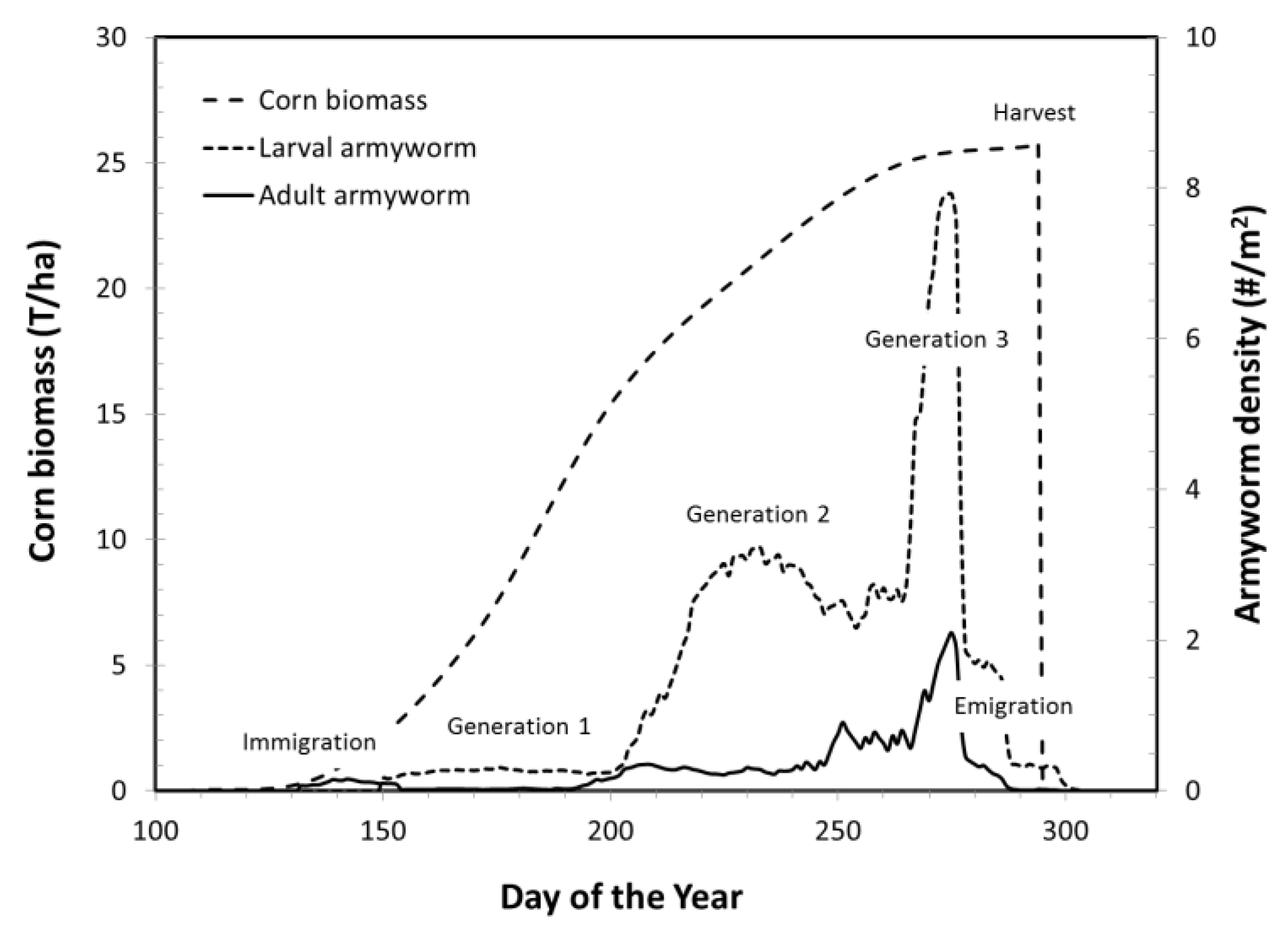
Figure 1 shows the trajectories of a typical simulation through the 2011 growing season in Wayne County, Ohio. Shown are the EPIC output of corn biomass and GILSYM output of population densities of adult and larval armyworm from immigration in May to emigration in late August and September. The simulations all follow this general pattern but details differ as resident species had populations present all year round and migrants were present for only part of the year. With the exception of univoltine stalk borer, the number of generations varied between species and between counties and years for a species.
The project simulated 200 years at 813 sites for all nine pest species. Such a large body of data generated by simulation is most effectively displayed as time-specific maps showing the spatial variation of variables. Maps (Figure 2, Figure 3, Figure 4, Figure 5 and Figure 6) showing the spatial distribution of crop production and insect damage without control measures, insect abundance, winter survival and number of generations are presented in four time periods (Period 1 = 1901–1950; Period 2 = 1951–2000; Period 3 = 2001–2050; Period 4 = 2051–2100). Table 2 summarizes the predicted consequences of climate warming for all nine species. We point out here that the damaging stage is species-specific: all but the egg stage of the beetles and potato leafhopper feed on their host plant whereas only the larval stage of the moths feed. Damage by armyworm, corn earworm and European corn borer larvae on corn all increased during the 20th century but other species’ impacts on yield were minor. Changes in life history characteristics were also mostly small; some up some down. Changes in the second half of the study were clearly different. Damage by all species increased, some, like European corn borer dramatically. These increases in predicted damage (absent insect control) resulted from both higher populations and longer exposure to the damaging stage. The longer exposure time was due to two causes: earlier onset of population growth due to developmental temperature thresholds and immigration occurring earlier. The longer growth period enabled an increase in the number of generations by all species but the obligate univoltine stalk borer. It should be noted that a mutation changing stalk borer’s voltinism would change this outcome, possibly increasing its crop damage.
We highlight results for four species to illustrate the spatial and temporal changes predicted by the model in the 21st century under the SRES-B1 scenario. We caution that in choosing the relatively benign SRES-B1 scenario, we ensured the responses of these species would likely remain within our experience. Some of the more extreme (and increasingly more likely) scenarios would likely take most known pest insects outside the bounds of our knowledge, rendering such a study highly speculative.
Most maps changed little from Period 1 to Period 2 reflecting the comparatively small increase in temperatures between 1901 and 1980. The most dramatic changes were seen in maps representing changes between Periods 2 and 3, while change between Periods 3 and 4 were, in most cases, small and in a few cases the changes reversed the trend of the previous half century. In no case were maps restored to their pre-2000 state. This pattern, little or no change, rapid change followed by minor change, was our expectation given the nature of the SRES-B1 scenario driving the models. The most significant finding of the simulations is that the anticipated productivity gains (Figure 2) from increased temperatures are offset by increased pest damage in both soybeans (Figure 3) and corn (not illustrated).
The specific avenues promoting changes in pest pressure differ somewhat between these representative species, reflecting the differences in their life systems. These differences are described below.
3.1. Species Responses
3.1.1. Stalk Borer Damage
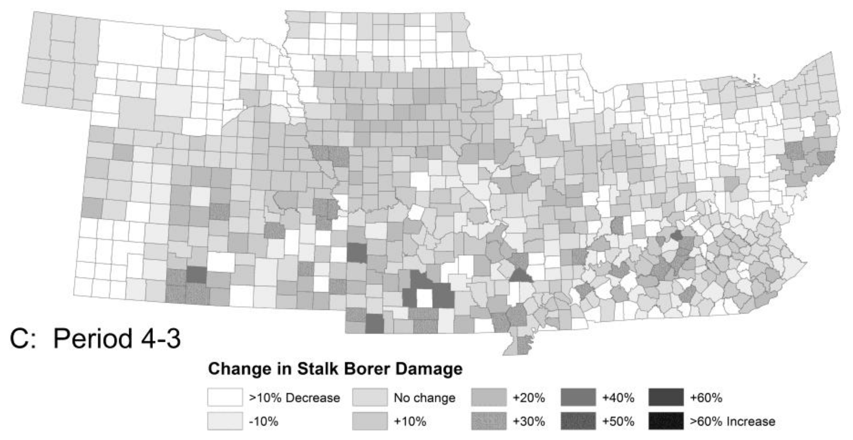
Stalk borer is currently a moderately serious pest throughout the southern part of the region and a sporadic problem in the northern tier of counties. The model predicted little change from Period 1 to 2 and a large increase in population and damage potential in Period 3 with a smaller increase in Period 4 (Figure 3). The northern tier of counties was predicted to see a doubling in population of stalk borer in Period 3 and a commensurate increase in potential crop damage. Southeastern Kansas, Southern Missouri and Kentucky could see little or no change in stalk borer damage potential. The largest increase in population was predicted for southern Iowa, northern Missouri and northeastern Kansas with damage potential increasing 60–70% from Period 2 to 3. This results from the northward movement of the area of maximal winter survival. However, overall survival across the region is expected to change little as the isoclines move north. The increase in damage potential results from the earlier onset of population growth. For this insect, the net effect for the region as a whole is likely to be small but could be locally extreme.
3.1.2. Armyworm Summer Population
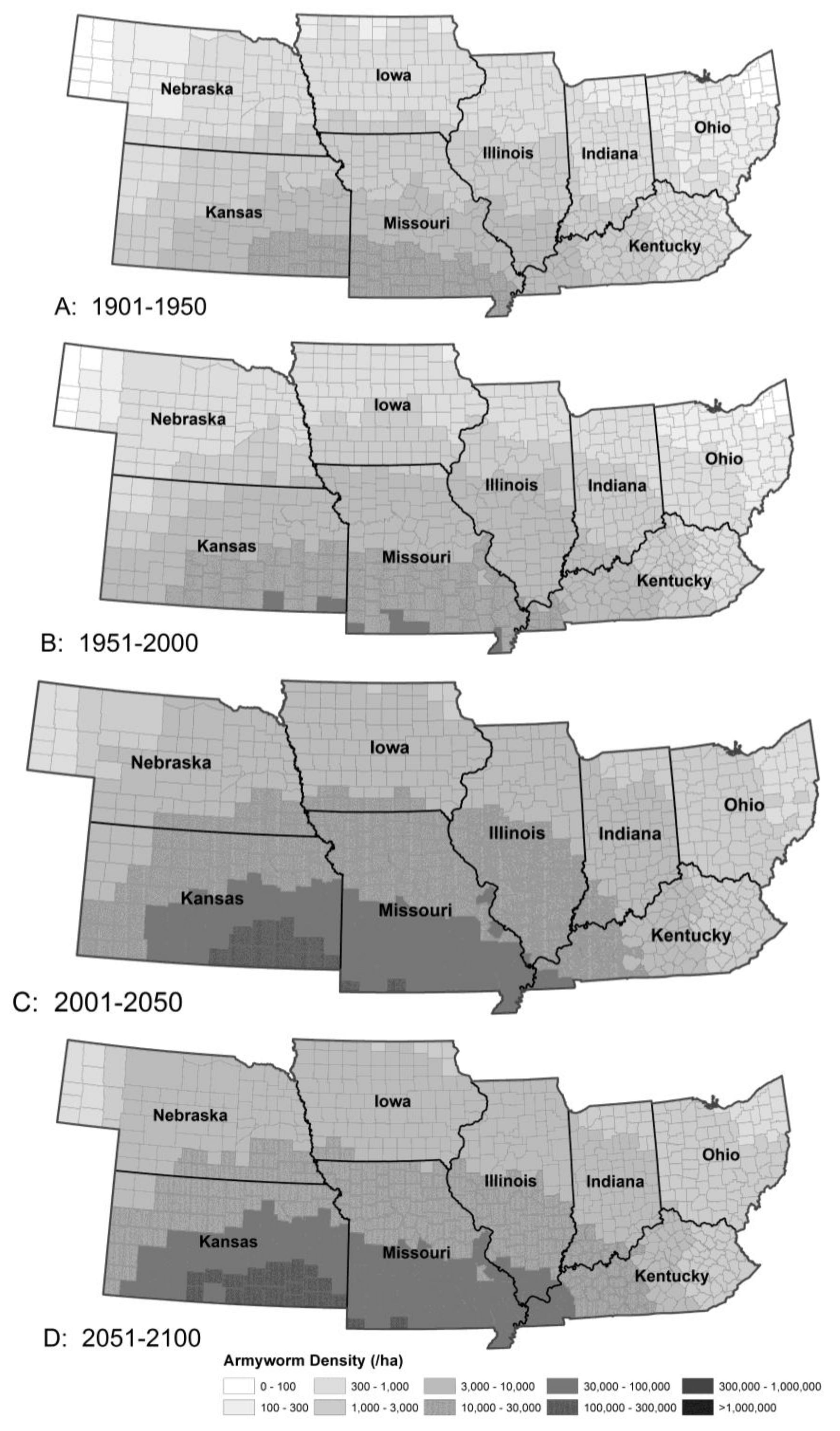
Armyworm invasions were predicted to occur earlier across the study area, with the largest change occurring at the western end, with Kansas in particular experiencing immigration of this species 1-week earlier with a 10–15% increase in the number of immigrants in Period 3 over Period 2. Increased temperatures combined with earlier invasions and longer growing season will permit an extra generation over most of the region. The extra generation will allow much higher populations to develop (Figure 4). Without control measures, most states would see a 50% increase in crop loss to armyworm in the next half century, with near 100% crop loss in some areas in most years. This increase in damage may be attributed to the increase in immigration rate combined with more rapid population growth resulting from the anticipated 20% increase in annual degree-day accumulations across most of the region.
3.1.3. Mexican Bean Beetle Survival
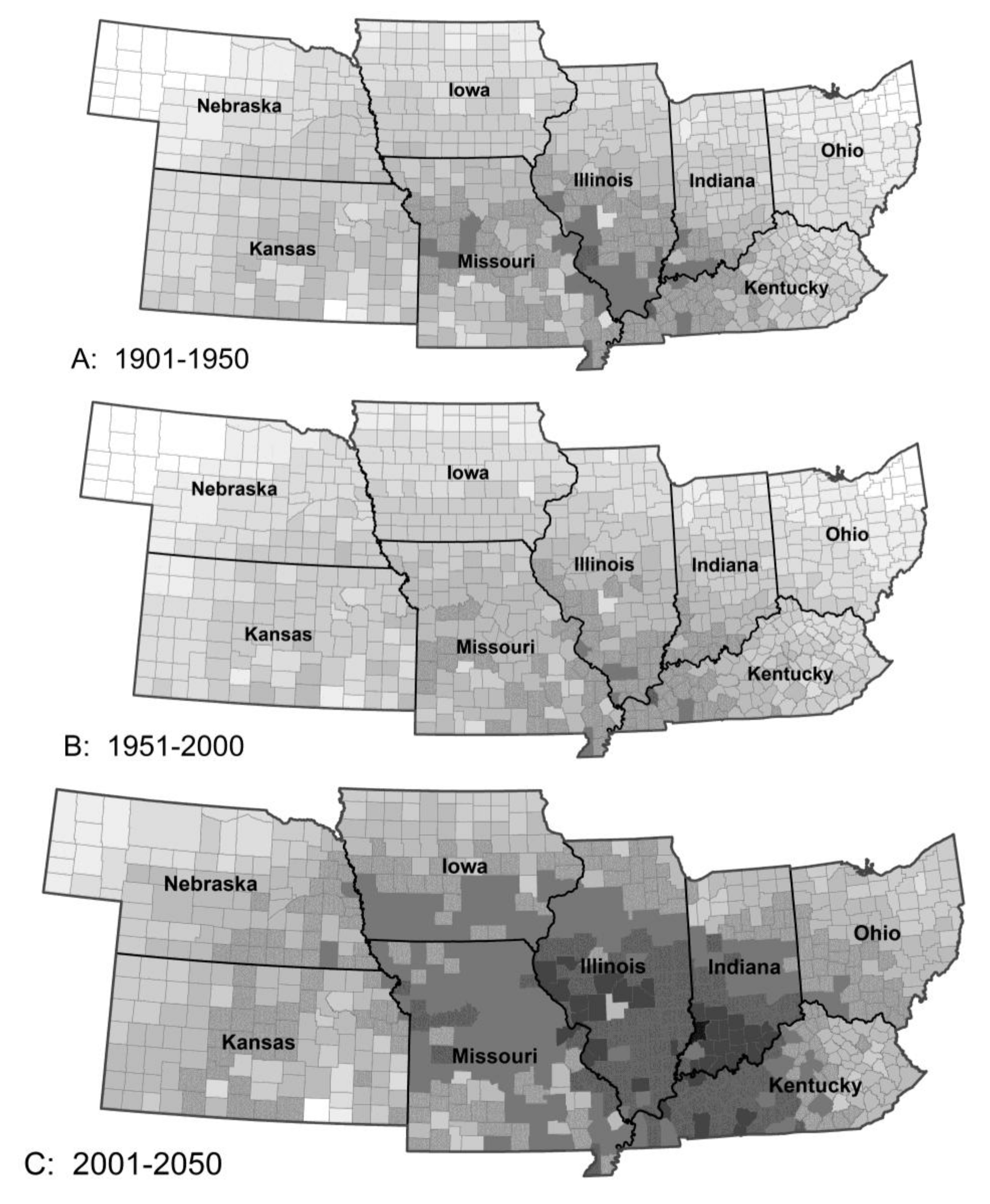
The model predicted only a small change in Mexican bean beetle population between Periods 1 and 2 in line with experience. Over the current century, the number of generations per year was predicted to increase from 2–3 to 4–5 over much of the range. This would result in substantial increases in population density over almost the entire range, except for NE Ohio and extreme NW Nebraska. The biggest increases in population were predicted for Kansas, Missouri and southern Iowa and Illinois. Unlike most of the other insects in the study, the biggest increase in population and damage potential was predicted in Period 4, not Period 3 as the beetle compensates for the higher summer temperatures. Overwinter survival is currently highest in southern Kansas, Missouri and Kentucky. By Period 3 peak overwinter survival will have moved north to central Illinois, southern Iowa and northeastern Kansas (Figure 5), which would increase the damage potential across the central part of the region.
3.1.4. Potato Leafhopper Generations
For all migrant species, the model predicts the arrival of immigrants up to two weeks earlier in Period 3 than in Period 2, resulting in at least one extra generation across the range. As a result, the model predicts a big increase in population and damage potential across the northern five states. The model predicted an increase in the number of generations per year in all species except the univoltine stalk borer. Potato leafhopper, a species with overlapping generations, is the starkest example, with the number of generations increasing only slightly in the 20th century but increasing dramatically during the 21st century (Figure 6). Its poor tolerance of high temperatures, will result in little change in pest status in Kentucky and even a slight reduction in southern Kansas and Missouri. Ohio is expected to see an increase in population and damage potential in Period 3 followed by a small decrease in period 4. The dependence of population growth on temperature is clearly evident in the relationship between number of generations and accumulated degree-days for this species (Figure 7).
3.2. Thermoperiodic Response to Climate Change
The strong relationship of generation number on heat units (Figure 7) suggests that day-degree accumulation may be the best predictor of increased potential pest pressure. Interestingly, the higher the developmental threshold, the larger the proportional change in degree-day accumulation, generation time and peak population (Figure 8) making insects with high developmental thresholds the more problematical as temperatures increase. This appears to be true for both resident and for migrant species. Potential pest pressure is strongly influenced by the number of generations, which is a function of the onset of population growth, which in turn depends on when the developmental threshold is exceeded. Population growth is starting earlier with an earlier break in diapause of overwintering stages and migratory insects arriving earlier and in larger numbers to their summer habitats. This will result in uncontrolled populations peaking later at higher densities for both immigrant and resident species, thus exposing crops to pests for longer and increasing pest pressure.
4. Discussion and Conclusions
All species have responded to climatic changes throughout their evolutionary history but of primary concern is the recent rapid rate of change demonstrated by Mann et al. [50]. During previous climate changes, species showed differential movements [51], rather than shifting together as suggested by many authors, including Darwin in The Origin of Species. Is it that pest status will not change because pest and crop will move poleward together? This was, in fact, the opinion of panels at granting agencies until recently, despite the warning of the 1989 US-EPA report on the likely impact of climate warming on agriculture [35].
Despite the simplifications made in this study, the key concept that climate warming will differentially impact pest insects and crop plants and therefore change their synchrony and interactions is clearly visible in these maps. The details of population abundance (numbers per hectare) and crop production (yield per hectare) are less important than their relative changes in distribution. The choice of the American Midwest as our study area was made to expose changes at regional scale and overcome the low signal-to-noise ratio imposed by population variation at local scales. The changes in regional climate are manifested, directly and indirectly, in changing position of isoclines of temperature and rainfall, resulting in consequential changes in the isoclines of crop and pest phenology, amount of crop damage and other indicators of the crop-pest interaction. For all insects modeled such shifts were especially pronounced in the first half of the 21st century, although the geographic details differed markedly between species. Our original hypothesis was that site-specific pest status would change, because we anticipated both increases and decreases in abundance locally. In most cases the model predicted that population increases occurred across our range but in stalk borer and potato leafhopper we found little or slightly negative change in abundance in the southern part of the range with the maximal isoclines moving northward as the “ideal” climate moved north.
Recent studies have questioned the early conclusions of possible increased crop productivity in the middle latitudes (e.g., [10]), although not on ecological grounds. Our results are in broad agreement with Long et al. [52] that an upper limit to crop productivity could be reached quickly with increased temperatures. Figure 2 shows the anticipated increase in productivity up to 2050 followed by a decline in the southern half of our region. Also, clearly visible in Figure 4 is the general poleward shift of the expected range of pests in the future if their climate adaptations remain unchanged (their “climate envelopes”) and the asymmetrical changes in distribution as the envelopes stretch poleward faster than they move north. To the extent that dispersal and resource availability allow, we expect insects to track these shifts with no time lag. In some species, responses to temperature may not occur or be moderated because of other limitations, such as day length responses or other restrictions to their life systems. Stalk borer’s obligate univoltinism is such a limitation, although increased overwintering survival and earlier break in diapause could select for changes to its life-history strategy. Countering this, we expect farmers to track these shifts by expanding or decreasing area planted as the areas of crop adaptation expand northward. Additionally, we would expect the mix of crop varieties to change and the introduction of new ones in response to changing needs. However, if the overall abundance of pests increases, as our results suggest, we will also expect increased reliance on pesticides, at least in the near term as new pest control tactics are developed.
Most insect pests are opportunists and often highly mobile, providing ample opportunity to exploit the changing climatic envelope. In general, warming-induced changes in distribution and abundance will be most evident in r-selected migrant and/or multivoltine species that can exploit rising temperatures by increasing the number of life cycles per year [37]. The multivoltine migratory armyworm (also black cutworm and corn earworm) showed a larger geographical displacement than the univoltine and resident stalk borer. Species like stalk borer with low adaptability and/or dispersal capability could be caught by the dilemma of climate-forced range change and low likelihood of finding distant habitats to colonize, although the availability of thousands of square miles of suitable host plants is unlikely to lead to their elimination as occasional agricultural pests. Needless to say, highly mobile species like armyworm that are adapted to explore large tracts for suitable habitat will have no difficulty in maintaining contact with suitable hosts.
4.1. Ecological Implications
Although insects with lower developmental thresholds become active earlier and will enjoy longer seasons, paradoxically it is the insects with higher thresholds that will present the larger problem for future pest control. High threshold species accumulate heat units faster and develop faster than low threshold species because the numerical increase in degree-days is roughly the same for low and high threshold species but the proportional change is greater for the latter. Thus, species that currently are not significant pests because they reach significant abundance levels after crop susceptibility may become more serious in the future. Knowledge of the thermoperiodic parameters for potential pests could enable us to anticipate which insects could emerge as pests in the future.
In a sense climate warming represents a “natural experiment” that could lead to a better understanding of what predisposes an insect to become a pest—beside the obvious point that r-selected species are more likely to be pests than K-selectors. We know relatively little about why particular insects become pests while close relatives in the same habitat do not and we know far less about the non-pest species than we do the pests. What shifts in synchrony, for example, could change pest status and what changes in climate, plant, soil and water interactions favor an insect becoming a pest? Detailed analysis of the impact of climate change on insect-plant interactions could lead to a better understanding of pest status. Our own results show that the impacts of the pests selected are likely to increase but not equally or uniformly either spatially or temporally. The life history constraints on the stalk borer suggest that its pest status could diminish in some areas as climate warming changes the distribution of the crops. The Mexican bean beetle is currently a comparatively easily controlled occasional pest that could become more important as larger and earlier populations develop. As global warming progresses, we may also expect to see some new pests emerging as changing conditions create new niches. Although we cannot predict which species will emerge as new pests, these general insights illuminate the life-history characteristics of such insects. By anticipating the preadaptations necessary to favor emergence as a new pest we should be able to plan for new pests and prepare ecologically sound management options.
4.2. Agricultural Implications
From a farmer’s point of view, the most significant causes of crop loss are physiological stresses caused by weather and pest abundance and duration. In broad acre crops plant competition from weeds is the number one pest stress but insect damage, both direct from herbivory and indirect via disease vectoring, is frequently serious and costly. The Mexican bean beetle and stalk borer results suggest that the main impact of weed competition in middle latitudes is likely to be an expansion of the range of species currently restricted by winter temperatures (e.g., purple nutsedge (Cyperus rotundus L.), bermudagrass (Cynodon dactylon (L.) Pers.) and johnsongrass (Sorghum halpense (L.) Pers.)) that will likely find a suitable habitat north of their current distributions. Clements & DiTomasso [53] documented range expansion of weeds from U.S. into Canada in response to elevated temperatures. They examined life history factors likely to promote northward expansion of range of four common weeds (Himalayan balsam (Impatiens glandulifera Royle), velvetleaf (Abutilon theophrasti Medik), Japanese knotweed (Fallopia japonica (Houtt.)) and johnsongrass). They concluded that the potential for evolutionary response to elevated temperature and CO2 was discernable in these species and likely to be replicated in others. It has been suggested that invasive species generally may be favored by elevated temperature and CO2 [54]. In South Africa, Bradley et al. [55] examined the potential geographic shift in suitable land for maize and wheat cultivation. As one might expect, they found that the areas suitable for cultivation of these staple crops would likely shift south; they also found that the total area available for them could shrink as the continent narrows southward. In addition to evolutionary effects on weed competition, pesticide efficacy might also suffer with increasing temperatures. Ziska [56] has identified several pathways for herbicide efficacy to be reduced in response to elevated temperatures and CO2: morphological and physiological adaptation of weeds to increased temperatures and CO2 could lead to increased weed vigor and fitness; persistence of herbicides on the crop could be reduced by elevated temperatures and increased frequency and/or severity of stormy weather would interfere with efficient pesticide application. These and other implications for weed management remain to be examined.
Analyses of the likely effects of climate change have all attempted to assess impact at a regional and in a few cases global, scale. These estimates have been derived from two approaches: point estimates scaled up to the desired region and spatially-explicit computations using mapping to display the results. Our approach is slightly different in that it replicates the point estimate approach at the county scale over a region comprising 813 counties. Schmitz et al. [57] suggested that “mapping approaches may paint a very conservative portrait of climate-change effects on ecosystems”. By employing climate and biological process models to generate generalized predictions, our results are conveniently presented as maps. It is likely that our mapped projections are indeed conservative but not because of the mapping approach. Our results are likely to be conservative because the well-known temperature-dependence of the rate of herbivory [58] is but one factor leading to changes in pest pressure under climate warming. An insect’s life-system will predispose its population response to climate change and those that have the most flexible life-systems are likely to take best advantage of climate warming. The maps (Figure 2, Figure 3, Figure 4, Figure 5 and Figure 6) clearly illustrate movement of the climate envelopes, implying changes in population dynamics and trophic interactions over the coming century.
The large range of elevations, soil types and growing seasons makes for quite large differences in planting and harvesting dates, fertilization and tillage practices. Over the same area, however, insect vital rates are unlikely to vary substantially except in direct response to ambient temperature, although agricultural practices can influence rates. But by fixing agricultural practices, we have removed this source of variation. High fecundity insects can evolve quickly (as exemplified by the rapid development of insecticide resistance in some species) and are expected to adapt quickly to climate change [59].
The appearance of a new pest frequently leads to an increased use of chemical pesticides with more frequent applications and the attendant environmental and economic costs. American agriculture uses billions of dollars of pesticides per year and there is increasing pressure to cut the amount and toxicity of pesticides. Part of the purpose of pesticides is to ensure that the crop is not lost to pests and like any insurance premium the price is paid to avoid unanticipated and extreme costs later. The appearance of new pests and the increase in severity or change in distribution of existing pests will require the payment of new insurance premiums in the form of pesticides until alternative pest management programs can be instituted. The value of anticipating those changes in pest status is measured in the billions of dollars in cash terms and is incalculable in environmental, societal and human health terms. It takes time to develop alternative pest management programs that reduce chemical use or employ alternative practices. The ability to anticipate new or changed pest pressures will permit research and extension to help farmers adapt quickly to the changing conditions with programs that permit prudent use of chemicals to the advantage of all concerned.
With the demonstrated earlier and longer growing seasons for both crops and pests, the best strategy for pest control is to disrupt the life cycle as much as possible. For migrant species overwintering outside our study region, management of the overwintering population is likely to be the best option but requires the cooperation of agencies in other states. Control of the immigrants following invasion is the other option, which will continue to emphasize predicting invasions and population growth combined with pesticides and insect resistant varieties. Later planting dates (i.e., not taking advantage of the longer growing season) could be a constructive approach to desynchronize the crop and pest. For resident species, managing the overwintering population is a viable option. The longer growing season opens more options for manipulating the timing of crops in order to reduce the susceptibility of the crop to pest attack. As phenological synchrony between insect and its host is often a significant factor in crop damage, choice of appropriate cultivars and planting dates could offset pest losses in some cases. However, these options may reduce the impact of one species but favor another. Thus, the choice of strategy will be site-specific. One strategy we believe would be effective throughout our study area is to increase the diversity of crops and the length of rotations. For example, planting wheat in the corn-soybean rotation has the advantage of lessening the effect of the stalk borer, decreasing the need for nitrogen fertilizer and decreasing the runoff rate and soil loss especially if coupled with no-till. An alternative would be to not take advantage of the longer growing season but to plant shorter season varieties of corn and soybeans. But this will inevitably sacrifice yield by reducing photosynthetic potential and shortening the grain fill period.
4.3. Broader Implications
The corn-soybean rotation has become the sole farming option for a large fraction of farmers across the Midwest since the 1970’s. Encouraging a move away from this practice will require not just agricultural and ecological decisions but also socio-economic pressures to change farming practices away from the widespread dependence on the corn-soybeans rotation. The evidence suggests that short rotations and lack of conservation measures exist in their highest percentages among tenant farmers because there is no incentive to improve the land owned by someone else. For tenant farms in particular, introducing winter wheat into their rotation is less attractive because fall planting requires that the corn and soybeans be harvested before September [60]. Short season varieties make winter crops much more feasible. Longer growing seasons could allow for more successful establishment of winter cover crops such as hairy vetch and mustards, to help diversify rotations while protecting soil from erosion, add organic matter and disrupt resident pest populations. However, farmers make their money on the principal crop, not cover crops, so use of shorter season, lower yielding varieties is not attractive. It is the long season varieties selected to respond well to high nitrogen inputs that yield the highest bushels per acre and therefore cash returns. However, it is these long-season varieties that may be subject to the highest level of uncertainty due to the increased frequency of environmental events creating uneven yearly yields in addition to greater pest exposure.
Our understanding of the likely changes in agricultural yield and pest pressure under climate change is fragmentary but growing but the likely environmental and societal problems resulting from these changes are almost completely unknown. It is likely that changes to crop production practices will be natural, physical and culturally “event” driven. Unanticipated changes to pest management needs that disrupt established pest management practices could jeopardize agricultural sustainability and environmental health by stimulating increased use of pesticides. It is conceivable that climate warming, which might increase temperate zone productivity in some commodities, at least in the short term, could ironically increase agriculture’s carbon footprint in proportion to the increase in temperature.
Acknowledgments
Salaries and research support provided by state and federal funds appropriated to The Ohio State University, Ohio Agricultural Research and Development Center. We thank two reviewers for their careful editing and thoughtful criticism of an earlier version. This project was funded by an OARDC SEEDS Interdisciplinary Competitive Grant.
Author Contributions
All four authors conceived and planned the project based on the preliminary work of Taylor and the late Ben Stinner in [35]. All four contributed to the writing: Herms on phenology and insect-plant relations, Cardina on crop protection and weed science and Moore on farm and social factors. Taylor developed the modeling environment and performed the number crunching.
Conflicts of Interest
The authors declare no conflict of interest.
References
- Schiermeier, Q. The costs of global warming. Nature 2006, 439, 374–375. [Google Scholar] [CrossRef] [PubMed]
- Smith, S.J.; Edmonds, J.; Hartin, C.A.; Mundra, A.; Calvin, K. Near-term acceleration in the rate of temperature change. Nat. Clim. Chang. 2015, 5, 333–336. [Google Scholar] [CrossRef]
- Seager, R.; Ting, M.; Held, I.; Kushnir, Y.; Lu, J.; Vecchi, G.; Huang, H.-P.; Harnik, N.; Leetmaa, A.; Lau, N.-C.; et al. Model projections of an imminent transition to a more arid climate in southwestern North America. Science 2007, 316, 1181–1184. [Google Scholar] [CrossRef] [PubMed]
- Allan, R.P.; Soden, B.J. Atmospheric warming and the amplification of precipitation extremes. Science 2008, 321, 1481–1484. [Google Scholar] [CrossRef] [PubMed]
- Thompson, L.G.; Mosley-Thompson, E.; Brecher, H.; Davis, M.; Leon, B.; Les, D.; Lin, P.N.; Mashiotta, T.; Mountain, K. Abrupt tropical climate change: Past and present. Proc. Natl. Acad. Sci. USA 2006, 103, 10536–10543. [Google Scholar] [CrossRef] [PubMed]
- Nicholls, R.J.; Cazenave, A. Sea-level rise and its impact on coastal zones. Science 2010, 328, 1517–1520. [Google Scholar] [CrossRef] [PubMed]
- Dukes, J.S.; Pontius, J.; Orwig, D.; Garnas, J.R.; Rodgers, V.L.; Brazee, N.; Cooke, B.; Theoharides, K.A.; Stange, E.E.; Harrington, R.; et al. Responses of insect pests, pathogens and invasive plant species to climate change in the forests of northeastern North America: What can we predict? Can. J. For. Res. 2009, 39, 231–248. [Google Scholar] [CrossRef]
- Maclean, I.M.D.; Wilson, R.J. Recent ecological responses to climate change support predictions of high extinction risk. Proc. Natl. Acad. Sci. USA 2011, 108, 12337–12342. [Google Scholar] [CrossRef] [PubMed]
- McMahon, S.M.; Parker, G.G.; Miller, D.R. Evidence for a recent increase in forest growth. Proc. Natl. Acad. Sci. USA 2010, 107, 3611–3615. [Google Scholar] [CrossRef] [PubMed]
- Lobell, D.B.; Schlenker, W.; Costa-Roberts, J. Climate trends and global crop production since 1980. Science 2011, 29, 616–620. [Google Scholar] [CrossRef] [PubMed]
- Asseng, S.; Ewert, F.; Martre, P.; Rötter, R.P.; Lobell, D.B.; Cammarano, D.; Kimball, B.A.; Ottman, M.J.; Wall, G.W.; White, J.W.; et al. Rising temperatures reduce global wheat production. Nat. Clim. Chang. 2015, 5, 143–147. [Google Scholar] [CrossRef]
- Schlenker, W.; Roberts, M.J. Nonlinear temperature effects indicate severe damages to U.S. crop yields under climate change. BioScience 2008, 58, 847–854. [Google Scholar] [CrossRef] [PubMed]
- Herms, D.A.; Mattson, W.J. The dilemma of plants: To grow or defend. Q. Rev. Biol. 1992, 67, 283–335. [Google Scholar] [CrossRef]
- Zvereva, E.L.; Kozlov, M.V. Consequences of simultaneous elevation of carbon dioxide and temperature for plant-herbivore interactions: A meta-analysis. Glob. Chang. Biol. 2006, 72, 27–41. [Google Scholar] [CrossRef]
- Hoekman, D. Turning up the heat: Temperature influences the relative importance of top-down and bottom-up effects. Ecology 2010, 91, 2819–2825. [Google Scholar] [CrossRef] [PubMed]
- Harrington, R.; Woiwod, I.; Sparks, T.H. Climate change and trophic interactions. Trend. Ecol. Evol. 1999, 14, 146–150. [Google Scholar] [CrossRef]
- Menzel, A.; Sparks, T.H.; Estrella, N.; Koch, E.; Aasas, A.; Ahass, R.; Alm-Tüsler, K.; Bissolli, P.; Braslavská, O.; Briede, A.; et al. European phenological response to climate change matches the warming pattern. Glob. Chang. Biol. 2006, 12, 1969–1976. [Google Scholar] [CrossRef]
- Schwartz, M.D.; Reiter, B.E. Changes in North American spring. Int. J. Clim. 2000, 20, 929–932. [Google Scholar] [CrossRef]
- Gibbs, J.P.; Breisch, A.R. Climate warming and calling phenology of frogs near Ithaca, New York, 1900–1999. Conserv. Biol. 2001, 15, 1175–1178. [Google Scholar] [CrossRef]
- Dunn, P.O.; Winkler, D.W. Climate change has affected the breeding date of tree swallows throughout North America. Proc. R. Soc. Lond. B 1999, 266, 2487–2490. [Google Scholar] [CrossRef]
- Jonzén, N.; Lindén, A.; Ergon, T.; Knudsen, E.; Vik, J.O.; Rubolini, D.; Piacentini, D.; Brinch, C.; Spina, F.; Karlsson, L.; et al. Rapid advance of spring arrival dates in long-distance migratory birds. Science 2006, 312, 1959–1961. [Google Scholar] [CrossRef] [PubMed]
- Roy, D.B.; Sparks, T.H. Phenology of British butterflies and climate change. Glob. Chang. Biol. 2000, 6, 407–416. [Google Scholar] [CrossRef]
- Parmesan, C.; Yohe, G. A globally coherent fingerprint of climate change impacts across natural systems. Nature 2003, 421, 37–42. [Google Scholar] [CrossRef] [PubMed]
- Fleming, R.A.; Tatchell, G.M. Shifts in the flight responses of British aphids: A response to climate warming? In Insects in a Changing Environment; Harrington, R., Stork, N.E., Eds.; Academic Press: London, UK, 1995; pp. 505–508. [Google Scholar]
- Buse, A.; Dury, S.J.; Woodburn, R.J.W.; Perrins, C.M.; Good, J.E.G. Effects of elevated temperature on multi-species interactions: The case of pedunculate oak, winter moth and tits. Funct. Ecol. 1999, 13, 74–82. [Google Scholar] [CrossRef]
- Sanz, J.J.; Potti, J.; Moreno, J.; Merino, S.; Frias, O. Climate change and fitness components of a migratory bird breeding in the Mediterranean region. Glob. Chang. Biol. 2003, 9, 461–472. [Google Scholar] [CrossRef]
- Winkler, D.W.; Dunn, P.O.; McCulloch, C.E. Predicting the effects of climate change on avian life-history traits. Proc. Natl. Acad. Sci. USA 2002, 99, 13595–13599. [Google Scholar] [CrossRef] [PubMed]
- Visser, M.E.; Adriaensen, F.; van Balen, J.H.; Blondel, J.; Dhondt, A.A.; van Dongen, S.; du Feu, C.; Ivankina, E.V.; Kerimov, A.B.; de Laet, J.; et al. Variable responses to large-scale climate change in European Parus populations. Proc. R. Soc. Lond. B 2003, 270, 367–372. [Google Scholar]
- Pounds, J.A.; Bustamante, M.R.; Coloma, L.A.; Consuegra, J.A.; Fogden, M.P.L.; Foster, P.N.; la Marca, E.; Masters, K.L.; Merino-Viteri, A.; Puschendorf, R.; et al. Widespread amphibian extinctions from epidemic disease driven by global warming. Nature 2006, 439, 161–167. [Google Scholar] [CrossRef] [PubMed]
- Woods, A.; Coates, K.D.; Hamann, A. Is an unprecedented Dothistroma needle blight epidemic related to climate change? BioScience 2005, 55, 761–769. [Google Scholar] [CrossRef]
- Ghandi, K.J.K.; Herms, D.A. Direct and indirect effects of alien insect herbivores on ecological processes and interactions in forest of eastern North America. Biol. Invasions 2010, 12, 389–405. [Google Scholar]
- Bentz, B.J.; Régnière, J.; Fettig, C.J.; Hansen, E.M.; Hayes, J.L.; Hicke, J.A.; Kelsey, R.G.; Negrón, J.F.; Seybold, S.J. Climate change and bark beetles of the western United States and Canada: Direct and indirect effects. BioScience 2010, 60, 602–613. [Google Scholar] [CrossRef]
- Cudmore, T.J.; Bjorklund, N.; Carroll, A.L.; Lindgren, S. Climate change and range expansion of an aggressive bark beetle: Evidence of higher beetle reproduction in naïve host tree populations. J. Appl. Ecol. 2010, 47, 1036–1043. [Google Scholar] [CrossRef]
- Volney, W.J.A.; Fleming, R.A. Climate change and impacts of boreal forest insects. Agric. Ecosyst. Environ. 2000, 82, 283–294. [Google Scholar] [CrossRef]
- Stinner, B.R.; Taylor, R.A.J.; Hammond, R.B.; Purrington, F.F.; McCartney, D.A.; Rodenhouse, N.; Barrett, G.W. Potential effects of climate change on plant-pest interactions. In The Potential Effects of Global Climate Change on the United States. Appendix C—Agriculture; Smith, J.B., Tirpak, D.A., Eds.; U.S. Environmental Protection Agency: Washington, DC, USA, 1989; p. 35. [Google Scholar]
- DeLucia, E.H.; Casteel, C.L.; Nabity, P.D.; O’Neill, B.F. Insects take a bigger bite out of plants in a warmer, higher carbon dioxide world. Proc. Natl. Acad. Sci. USA 2009, 105, 1781–1782. [Google Scholar] [CrossRef] [PubMed]
- Chen, S.; Fleischer, S.J.; Tobin, P.C.; Saunders, M.C. Projecting insect voltinism under high and low greenhouse gas emission conditions. Environ. Entomol. 2011, 40, 505–515. [Google Scholar] [CrossRef] [PubMed]
- Trumble, J.T.; Butler, C.D. Change will exacerbate California’s insect pest problems. Calif. Agric. 2009, 63, 73–78. [Google Scholar] [CrossRef]
- North American Plant Protection Organization (NAPPO). Climate Change and Pest Risk Analysis; Discussion Paper. Available online: https://www.nappo.org/files/4814/3781/8174/Climate_Change_Discussion_DocumentRev-07-08-12-e.pdf (accessed on 10 December 2017).
- Lindroth, R.L. Impacts of elevated atmospheric CO2 and O3 on forests: Phytochemistry, trophic interactions and ecosystem dynamics. J. Chem. Ecol. 2010, 36, 2–21. [Google Scholar] [CrossRef] [PubMed]
- Sharpley, A.N.; Williams, J.R. (Eds.) EPIC—Erosion/Productivity Impact Calculator: 1. Model Documentation; United States Department of Agriculture: Washington, DC, USA, 1990.
- Gassman, P.W.; Williams, J.R.; Benson, V.W.; Izaurralde, R.C.; Hauck, L.; Jones, C.A.; Atwood, J.D.; Kiniry, J.; Flowers, J.D. Historical Development and Applications of the EPIC and APEX Models; Center for Agricultural and Rural Development, Iowa State University: Ames, IA, USA, 2005. [Google Scholar]
- Rasche, L.; Taylor, R.A.J. A generic pest submodel for use in integrated assessment models. Trans. ASABE 2017, 60, 147–158. [Google Scholar]
- Source of County Soils Data. Available online: https://datagateway.nrcs.usda.gov (accessed on 10 December 2017).
- Source of Historical Weather Data. 1901–2000. Available online: https://www.ncdc.noaa.gov (accessed on 10 December 2017).
- Source of Predicted Weather Data. 2001–2100. Available online: http://nomads.gfdl.noaa.gov (accessed on 10 December 2017).
- Intergovernmental Panel on Climate Change (IPCC). Climate Change 2007: The Physical Science Basis: Contribution of Working Group I to the Fourth Assessment Report of the Intergovernmental Panel on Climate Change; Cambridge University Press: Cambridge, UK, 2007. [Google Scholar]
- Stouffer, R.J.; Broccoli, A.J.; Delworth, T.L.; Dixon, K.W.; Gudgel, R.; Held, I.; Hemler, R.; Knutseon, T.; Lee, H.-C.; Schwartzkopf, M.D.; et al. GFDL’s CM2 Global coupled climate models. Part IV: Idealized climate response. J. Clim. 2006, 19, 723–740. [Google Scholar] [CrossRef]
- Taylor, R.A.J.; Shields, E.J. Revisiting potato leafhopper, Empoasca fabae, migration: Implications in a world where invasive insects are all too common. Am. Entomol. 2018, in press. [Google Scholar]
- Mann, M.E.; Bradley, R.S.; Hughes, M.K. Global-scale temperature patterns and climate forcing over the past six centuries. Nature 1998, 392, 779–787. [Google Scholar] [CrossRef]
- Root, T.L.; Price, J.T.; Hall, K.R.; Schneider, S.H.; Rosenzweig, C.; Pounds, J.A. Fingerprints of global warming on wild animals and plants. Nature 2003, 421, 57–60. [Google Scholar] [CrossRef] [PubMed]
- Long, S.P.; Ainsworth, E.A.; Leakey, A.D.B.; Nösberger, J.; Ort, D.R. Food for thought: Lower-than-expected crop yield stimulation with rising CO2 concentrations. Science 2006, 312, 1918–1921. [Google Scholar] [CrossRef] [PubMed]
- Clements, D.R.; DiTommaso, A. Predicting weed invasion in Canada under climate change: Evaluating evolutionary potential. Can. J. Plant Sci. 2012, 92, 1013–1020. [Google Scholar] [CrossRef]
- Ziska, L.H. Climate change and plant protection: Emerging viral and weed threats. Abstracts of Special Session at the 2011 APS-IPPC Joint Meeting in Honolulu, Hawaii. Phytopathology 2011, 101, S240. [Google Scholar]
- Bradley, B.A.; Estes, L.D.; Hole, D.G.; Holness, S.; Oppenheimer, M.; Turner, W.R.; Beukes, H.; Schulze, R.E.; Tadross, M.A. Predicting how adaptation to climate change could affect ecological conservation: Secondary impacts of shifting agricultural suitability. Divers. Distrib. 2012, 18, 425–437. [Google Scholar] [CrossRef]
- Ziska, L.H. The role of climate change and increasing atmospheric carbon dioxide on weed management: Herbicide efficacy. Agric. Ecosyst. Environ. 2016, 231, 304–309. [Google Scholar] [CrossRef]
- Schmitz, O.J.; Post, E.; Burns, C.E.; Johnston, K.M. Ecosystem responses to global climate change: Moving beyond color mapping. BioScience 2003, 53, 1199–1205. [Google Scholar] [CrossRef]
- Watt, A.D.; Whittaker, J.B.; Docherty, M.; Brooks, G.; Lindsay, E.; Salt, D. The impact of elevated atmospheric CO2 on insect herbivores. In Insects in a Changing Environment; Harrington, R., Stork, N.E., Eds.; Academic Press: London, UK, 1995; pp. 198–217. [Google Scholar]
- Bale, J.S.; Masters, G.J.; Hodkinson, I.D.; Awmack, C.; Bezemer, T.M.; Brown, V.K.; Butterfield, J.; Buse, A.; Coulson, J.C.; Farrar, J.; et al. Herbivory in global climate change research: Direct effects of rising temperature on insect herbivores. Glob. Chang. Biol. 2002, 8, 1–16. [Google Scholar] [CrossRef]
- Parker, J.S.; Moore, R.; Weaver, M. Land tenure as a variable in community based watershed projects: Some lessons from the Sugar Creek watershed, Wayne and Holmes County, Ohio. Soc. Nat. Res. 2007, 20, 815–833. [Google Scholar] [CrossRef]
Figure 1.
In a typical model run, the crop biomass increased during the spring and summer and was harvested in September or October; crop biomass is shown without crop loss to pests. This simulation is of armyworm on corn in Wayne County, Ohio in 2011. Armyworm adults immigrated in May, and developed three generations before adults entered reproductive diapause in August and emigrated. Yield loss was calculated at harvest based on the magnitude and timing of the larval population density.

Figure 2.
Model predictions for soybean production in the absence of pest pressure: Period 1 (A), Period 2 (B), Period 3 (C) and Period 4 (D). The model predicted increasing temperatures from Period 2 to 3 will lead to a modest increase in yield followed by a decline in the latter part of the 21st century (Period 3 to 4), resulting from heat stress and changing rainfall patterns. Note the northward movement of maximal productivity. The changes in corn productivity between periods were similar although the spatial details differed.

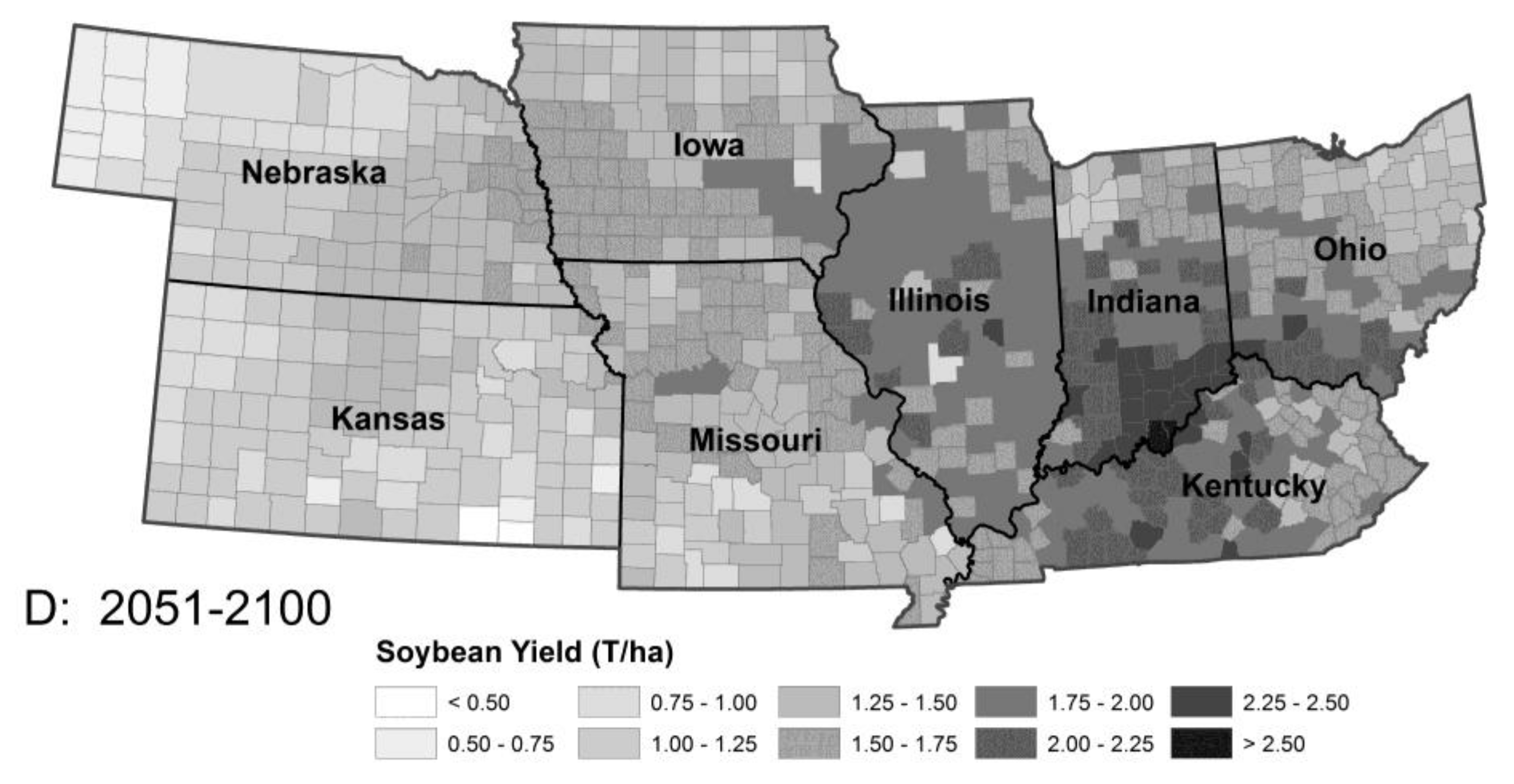
Figure 3.
The model predicted little change in crop damage (A) by stalk borer (without insecticides) from Period 1 to 2, except for an area in Eastern Kentucky, large increases in crop damage (B) across the region from Period 2 to 3 and a small recovery (C) from Period 3 to 4. Damage by Mexican bean beetle was similar in overall pattern but differed in detail.
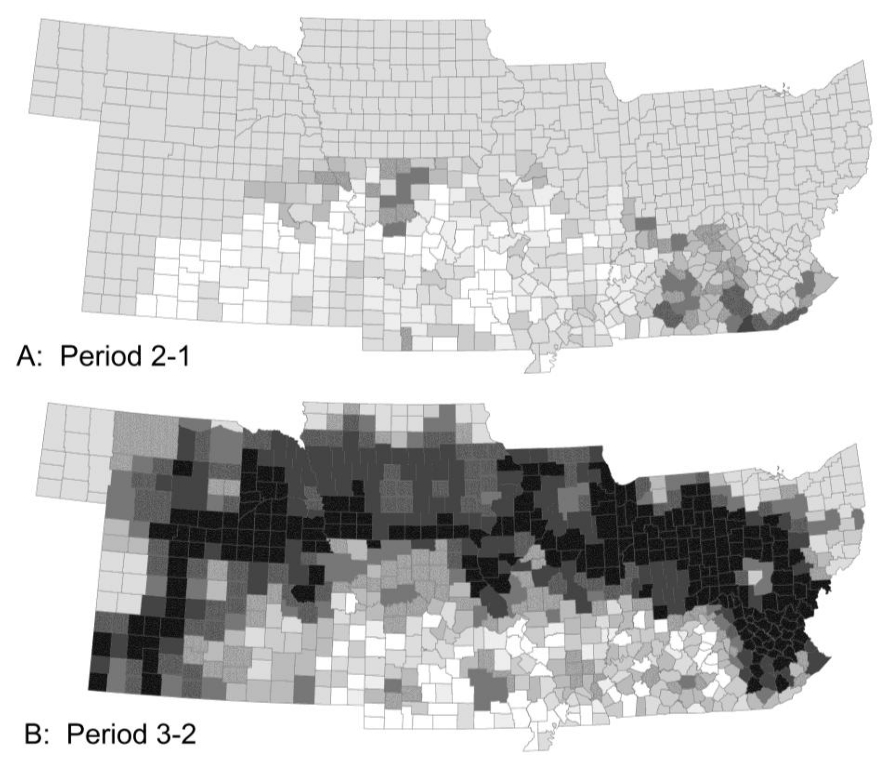

Figure 4.
The model predicted essentially no change in armyworm summer abundance from Period 1 (A) to Period 2 (B), an increase from Period 2 to 3 (C) with local changes only in abundance from Period 3 to 4 (D). The distribution and trajectory of back cutworm and corn earworm were similar.
Figure 4.
The model predicted essentially no change in armyworm summer abundance from Period 1 (A) to Period 2 (B), an increase from Period 2 to 3 (C) with local changes only in abundance from Period 3 to 4 (D). The distribution and trajectory of back cutworm and corn earworm were similar.

Figure 5.
The model predicted almost no climate-related change in percent of Mexican bean beetle surviving the winter from Period 1 to 2 (A) but a large increase in winter survival from Period 2–3 (B) and a shift in the isoclines as well as a small increase in survival from Period 3–4 (C). The pattern of survival of bean leaf beetle and European corn borer were similar although the values differed with European corn borer having the overall biggest increase in overwintering survival and bean leaf beetle the smallest.
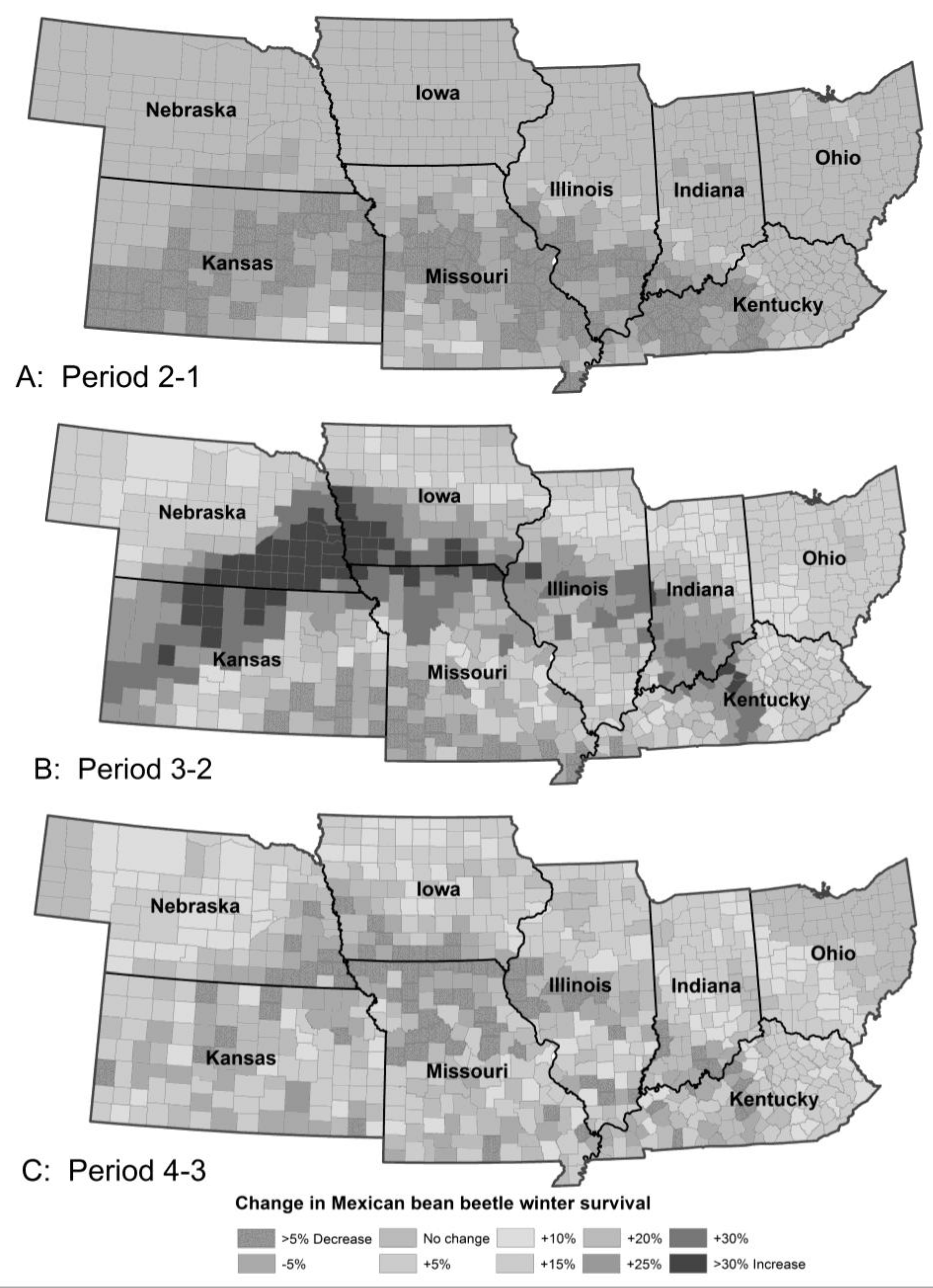
Figure 6.
The model predicted little change in number of generations per year of potato leafhopper between Periods 1 (A) and 2 (B) with a dramatic increase in the number of generations in the northern and western counties in Period 3 (C) and increased number of generations everywhere in Period 4 (D).
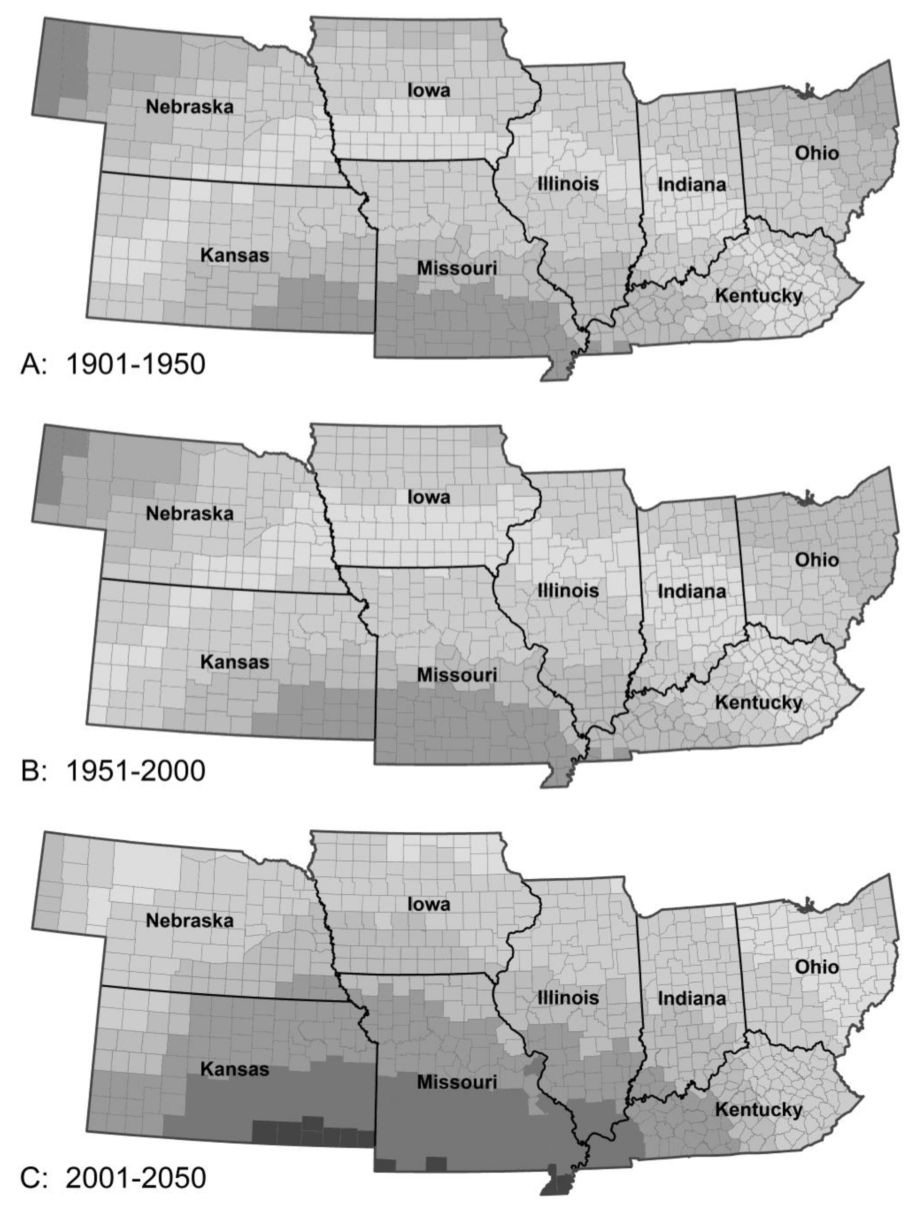

Figure 7.
All changes in the dynamics of the crop-pest system can be traced to the changes in the heat accumulations by the pest insects. The number of potato leafhopper generations per year is directly proportional to the total degree-days accumulated above its developmental threshold of 8.5 °C. With the exception of univoltine stalk borer, all species exhibited an increase in generations in proportion to accumulated degree-days.
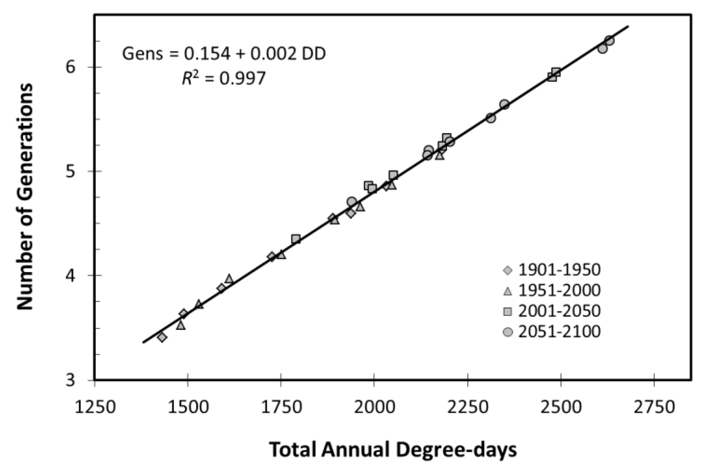
Figure 8.
The percentage change (±standard error) in degree-day accumulations increases with developmental threshold. Both the intercept and the gradients increased when Period 1 is compared with Periods 2, 3 and 4. The largest increases in degree-day accumulations occurred in the interval Period 2–3. Data presented here are for all nine species studied, each with a different developmental threshold.


Table 1.
Insect life history characteristics programmed into the Generalized Insect Life-SYstem Model (GILSYM).
Table 1.
Insect life history characteristics programmed into the Generalized Insect Life-SYstem Model (GILSYM).
| Pest Species | Status | Crops | Fecundity: Total Eggs; Eggs/Day | Feeding Rate (mg/Day) | Damage Potential | Thresholds (°C) | Degree-Days to Adult | Adult Lifespan (Days) | ||
|---|---|---|---|---|---|---|---|---|---|---|
| Beans | Corn | Upper | Lower | |||||||
| Coleoptera | ||||||||||
| Bean leaf beetle | R | B | 350; 35 | 3.5 | 6.5 | - | 30 | 10 | 490 | 30 |
| (Ceratoma trifurcata) | ||||||||||
| Mexican bean beetle | R | B | 300; 30 | 3.5 | 12.5 | - | 30 | 11.5 | 385 | 20 |
| (Epilachna varivestis) | ||||||||||
| Lepidoptera | ||||||||||
| Armyworm | M | C | 200; 20 | 25 | - | 25 | 30 | 9 | 610 | 15 |
| (Pseudaletia unipuncta) | ||||||||||
| Black cutworm | M | C | 100; 10 | 8 | - | 10 | 35 | 8 | 350 | 30 |
| (Agrotis ipsilon) | ||||||||||
| Corn earworm | RM | BC | 200; 40 | 6 | 8 | 50 | 35 | 12.5 | 480 | 20 |
| (Heliothis zea) | ||||||||||
| European corn borer | R | BC | 300; 30 | 8 | 8 | 3 | 30 | 9.5 | 660 | 15 |
| (Ostrinia nubilalis) | ||||||||||
| Stalk borer | R | BC | 750; 75 | 20 | 5 | 5 | 30 | 9 | 1250 | 10 |
| (Papaipama nebris) | ||||||||||
| Velvetbean caterpillar | M | B | 300; 30 | 25 | 25 | - | 35 | 11 | 485 | 20 |
| (Anticarsia gemmatalis) | ||||||||||
| Homoptera | ||||||||||
| Potato leafhopper | M | B | 600; 20 | 1.5 | 6.5 | - | 30 | 8.5 | 415 | 35 |
| (Empoasca fabae) | ||||||||||
Key: B = soybeans; C = corn; M = migratory; R = resident. Stalk borer is obligate univoltine; all other insects are capable of completing more than one generation per year. Black cutworm, corn earworm and stalk borer feed primarily on grasses but will feed on beans doing little damage normally. Overwintering adult Mexican bean beetles live for up to 5 months.
Table 2.
Changes in predicted outcomes and insect life history characteristics.
| Pest Species & Crop | Change from 1901 to 2000 | Change from 1901 to 2100 | |||||||||||
|---|---|---|---|---|---|---|---|---|---|---|---|---|---|
| Yield | Damage | Expose | Peak | Initial | Gens | Yield | Damage | Expose | Peak | Initial | Gens | ||
| (%) | (%) | (days) | (days) | (% or d) | (%) | (%) | (%) | (days) | (days) | (% or d) | (%) | ||
| Bean leaf beetle | B | 3.1 | −8.4 | −1.4 | −3.4 | −0.9% | −8.4 | 37 | 430 | 15.3 | 18.5 | 13.3% | 73.4 |
| Mexican bean beetle | B | 3.1 | −2.1 | −1.7 | −1.6 | −2.5% | 0.8 | 37 | 42 | 2.6 | 16.6 | 4.4% | 7.8 |
| Armyworm | C | 2.9 | 30.1 | 2.6 | 5.0 | −2.5 d | 7.1 | 21 | 100 | 14.4 | 19.2 | −7.0d | 26.0 |
| Black cutworm | C | 2.9 | 4.7 | 4.5 | 5.5 | −3.6 d | 5.6 | 21 | 16 | 18.9 | 18.8 | −9.1d | 23.8 |
| Corn earworm | C | 3.1 | 0 | 1.3 | 1.1 | 0.9 d | 1.3 | 37 | 480 | 14.2 | 32.8 | −7.1d | 31.6 |
| B | 2.9 | 42.9 | 4.5 | 7.5 | −3.4 d | 8.6 | 21 | 136 | 14.2 | 30.7 | −8.2d | 29.0 | |
| European corn borer | C | 3.1 | 5.0 | 2.7 | −0.1 | 2.6% | 1.2 | 37 | 1000 | 35.4 | 39.2 | 17.6% | 28.4 |
| B | 2.9 | 38.6 | 11.7 | 4.7 | 1.9% | 7.7 | 21 | 800 | 36.7 | 37.8 | 18.7% | 27.5 | |
| Stalk borer | C | 3.1 | 1.7 | 0.1 | 0.9 | 0.6% | 0 | 37 | 165 | −13.8 | 60.1 | 1.5% | 0 |
| B | 2.9 | 0.4 | −4.3 | 1.6 | 1.1% | 0 | 21 | 153 | −12.3 | 59.2 | 1.4% | 0 | |
| Velvetbean caterpillar | B | 3.1 | 2.0 | 2.7 | 1.0 | 0.5 d | 0.9 | 37 | 326 | 15.4 | 21.1 | −9.9d | 34.6 |
| Potato leafhopper | B | 3.1 | 4.1 | 1.3 | 1.1 | 1.5 d | 1.0 | 37 | 155 | 12.8 | 27.4 | −8.1d | 27.5 |
Key: B = soybeans; C = corn. Yield: Change in crop yield without insect damage; Damage: Change in crop lost to herbivory without insect control; Expose: Change in the number of days the crop was exposed to herbivory; Peak: Change in population/hectare of damaging stage at the peak population without insect control; Initial: Change in overwinter survival (%) for residents or timing of immigration for migrants (d); negative number indicates earlier immigration resulting in population establishment; Gens: Change in the number of generations per year. Statistics are averaged over all 813 counties.
© 2018 by the authors. Licensee MDPI, Basel, Switzerland. This article is an open access article distributed under the terms and conditions of the Creative Commons Attribution (CC BY) license (http://creativecommons.org/licenses/by/4.0/).
Share and Cite
MDPI and ACS Style
Taylor, R.A.J.; Herms, D.A.; Cardina, J.; Moore, R.H. Climate Change and Pest Management: Unanticipated Consequences of Trophic Dislocation. Agronomy 2018, 8, 7. https://doi.org/10.3390/agronomy8010007
AMA Style
Taylor RAJ, Herms DA, Cardina J, Moore RH. Climate Change and Pest Management: Unanticipated Consequences of Trophic Dislocation. Agronomy. 2018; 8(1):7. https://doi.org/10.3390/agronomy8010007
Chicago/Turabian StyleTaylor, R. A. J., Daniel A. Herms, John Cardina, and Richard H. Moore. 2018. "Climate Change and Pest Management: Unanticipated Consequences of Trophic Dislocation" Agronomy 8, no. 1: 7. https://doi.org/10.3390/agronomy8010007
Note that from the first issue of 2016, this journal uses article numbers instead of page numbers. See further details here.