Phosphorus and Nitrogen Yield Response Models for Dynamic Bio-Economic Optimization: An Empirical Approach


1
Department of Economics, University of Helsinki, Latokartanonkaari 7, 00790 Helsinki, Finland
2
Natural Resources Institute Finland (LUKE), Bioeconomy and environment/Sustainability Science and Indicators, Itäinen Pitkäkatu 4 A, 20520 Turku, Finland
3
Natural Resources Institute Finland (LUKE), Management and Production of Renewable Resources/Environmental Impact, Tietotie 4, FI-31600 Jokioinen, Finland
*
Author to whom correspondence should be addressed.
Agronomy 2018, 8(4), 41; https://doi.org/10.3390/agronomy8040041
Submission received: 24 January 2018
/
Revised: 26 March 2018
/
Accepted: 29 March 2018
/
Published: 31 March 2018
(This article belongs to the Special Issue Plant Mineral Nutrition: Principles and Perspectives)
Abstract
:Nitrogen (N) and phosphorus (P) are both essential plant nutrients. However, their joint response to plant growth is seldom described by models. This study provides an approach for modeling the joint impact of inorganic N and P fertilization on crop production, considering the P supplied by the soil, which was approximated using the soil test P (STP). We developed yield response models for Finnish spring barley crops (Hordeum vulgare L.) for clay and coarse-textured soils by using existing extensive experimental datasets and nonlinear estimation techniques. Model selection was based on iterative elimination from a wide diversity of plausible model formulations. The Cobb−Douglas type model specification, consisting of multiplicative elements, performed well against independent validation data, suggesting that the key relationships that determine crop responses are captured by the models. The estimated models were extended to dynamic economic optimization of fertilization inputs. According to the results, a fair STP level should be maintained on both coarse-textured soils (9.9 mg L−1 a−1) and clay soils (3.9 mg L−1 a−1). For coarse soils, a higher steady-state P fertilization rate is required (21.7 kg ha−1 a−1) compared with clay soils (6.75 kg ha−1 a−1). The steady-state N fertilization rate was slightly higher for clay soils (102.4 kg ha−1 a−1) than for coarse soils (95.8 kg ha−1 a−1). This study shows that the iterative elimination of plausible functional forms is a suitable method for reducing the effects of structural uncertainty on model output and optimal fertilization decisions.

1. Introduction
The motivation for using nutrient inputs in agriculture more efficiently has never been greater than it is currently. This motivation originates from increased demand for food, finite available arable land and fertilizer material resources, expected increase in energy costs, growing public concerns related to environmental effects of agriculture, and the need for improved productivity and profitability of cropping systems [1,2]. The changing climate and long-term socioeconomic trends are anticipated to alter the future challenges in agricultural production in complex, yet uncertain and possibly controversial ways [3,4,5]. Sustained supply and long-term efficiency in the use of inorganic fertilizers, namely nitrogen (N) and phosphorus (P), will be critical for meeting the increasing global food demand [6].
Bio-economic models can be used as tools to study economically and environmentally sound fertilizer inputs in crop production. Multiple empirical models have been developed to separately capture yield response to N inputs [7,8,9], and to P inputs [10,11,12], and as a response to plant-available soil P [13,14,15]. Both the response to P fertilizer and soil P dynamics have been incorporated into an economic analysis of nutrient inputs [16,17]. Lambert et al. [18] studied spatially and temporally optimal fertilizer inputs for soybean and corn rotation. To the best of our knowledge, this is the only prior study that simultaneously considered the N and P inputs with P carryover in an economic analysis of crop production. The joint impact of N and P inputs on crop yield was explicitly considered in dynamic crop growth simulation models, such as DAISY [19], HYPE [20], APSIM [21], and EPIC [22,23], and in decision support systems for agrotechnology transfer like DSSAT [24]. Although these models provide a rich and detailed description of the processes driving the yield response, they are not directly suited to dynamic economic optimization due to the large number of state variables and the extensive data requirements [25].
The existing literature investigating the joint impacts and dynamic feedbacks associated with economically optimal N and P fertilization is scarce, despite its importance for crop production. The obvious reason for the lack of this type of study is the need for extensive and long-term data from field experiments that capture the weather-induced variation in the impacts of N and P inputs and soil quality on crop growth [26]. Such field experiments are expensive to conduct [27]. Yield response modeling is a data-intensive process, as empirical data is needed for both building and validating the model [28]. In Finland, a long tradition of N and P fertilizer field experiments exists, motivated by the challenging agro-climatic production conditions due to the Nordic location and natural scarcity of P in the soil [9,11,12,29,30,31]. As a result of these experiments, extensive empirical data for main cereals and different soil textures have been accumulated over five decades. However, identifying the effects of the individual nutrients from the compound fertilizer experimental data is difficult due to the complex interactions between N and P, and the general multicollinearity problem [32].
The objective of this study was to estimate and validate yield response models suitable for simultaneous optimization of inorganic P and N fertilization for spring barley (Hordeum vulgare L.). The models were developed for the following two soil texture groups: clay soils and coarse-textured mineral soils. The plant-available phosphorus dynamics (soil test phosphorus: STP) were included in the modeling to allow for the examination of temporally optimal fertilization paths. The models were designed for optimizing long-term farm level N and P fertilization decisions. The relative importance of different sources of uncertainty, including structural and parametric uncertainty, were evaluated. The robustness of various model specifications for economic optimization was also assessed.
2. Materials and Methods
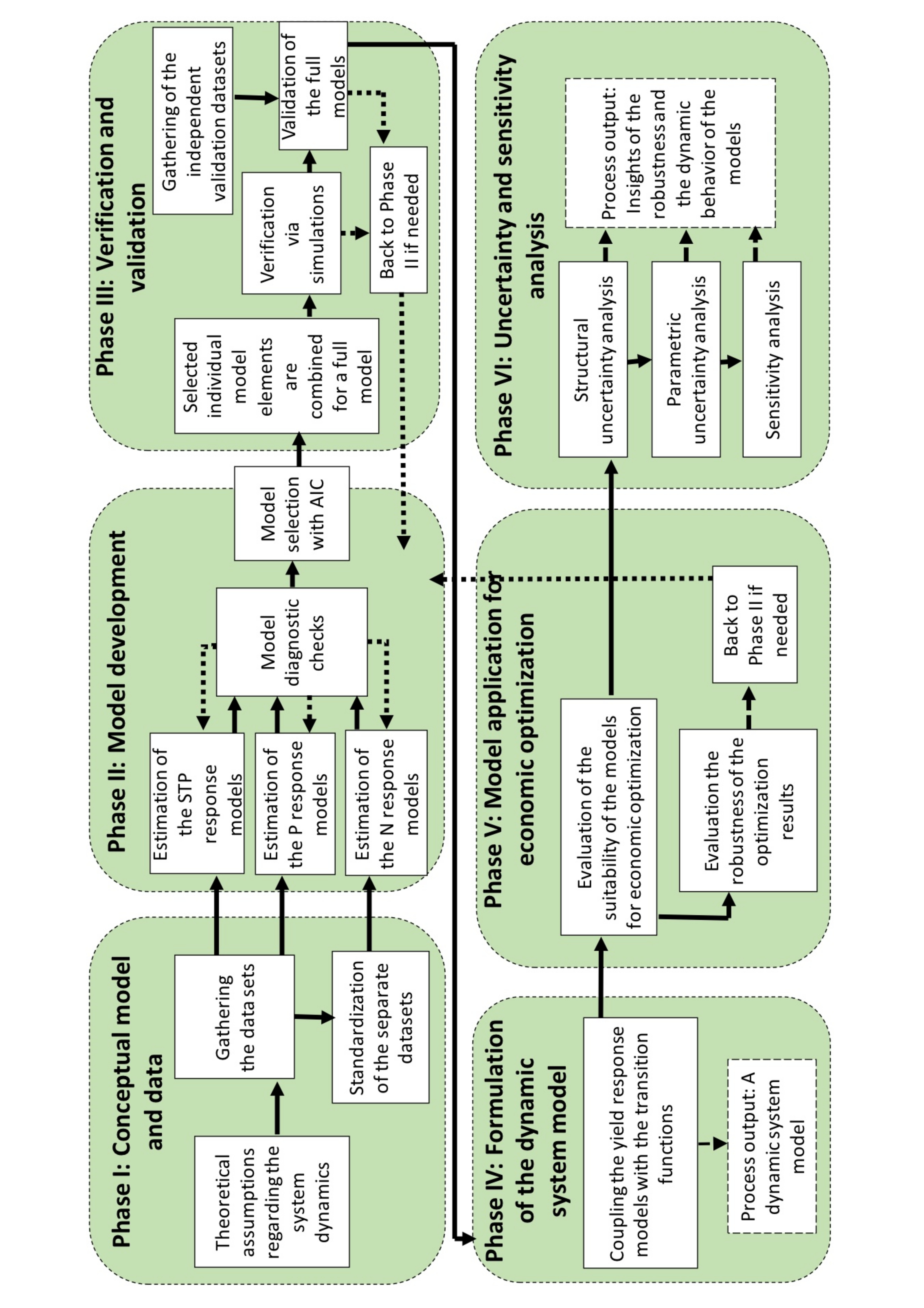
In this study, an iterative approach to model building was applied [33,34,35]. In the first phase (Figure 1), the conceptual model was developed and the available and relevant data for model estimation and validation were gathered. The second and the third phases included model estimation, verification, and validation. In the fourth phase, the yield response model was coupled with the transition function describing STP dynamics. In the fifth phase, the dynamic system model was applied for economic optimization. Finally, the sixth phase included uncertainty and sensitivity analyses.
2.1. Phase I: Conceptual Model and Data
Our conceptual model was built on the following findings from the literature: (1) the amounts of nutrients in mineral fertilizers that should be applied depend on the nutrient requirement of a crop and the nutrient supply from the soil [2]; (2) inputs of inorganic P and N fertilizers have a direct positive effect on annual yield up to a certain level, as the availability of N and P are typically the most limiting factors for crop growth [37,38,39]; (3) P fertilization has a direct positive effect on STP due to the accumulation of P in the soil if the application exceeds the P removal by the harvest [40,41,42]; (4) N fertilization has an indirect negative effect on P balance by positively and indirectly affecting crop P uptake, meaning that the P is removed annually from the system in the harvested yield; (5) a positive association exists between STP and crop yield [14,15,43,44]; and (6) P fertilizer responses are lower for higher STP levels as P is available for plants from the existing reserve in soil. Consequently, yield responses to P fertilization are probable for STP classes ranging from poor to fair, whereas the responses become improbable for STP classes ranging from satisfactory to excessive [12,45,46]. The applied ranges for the STP classes on coarse soils are here as follows: poor, 0–3; rather poor, 3–6; fair, 6–12; satisfactory, 12–20; good, 20–33; high, 33–50; excessive, >50 mg l−1 a−1. On clay soils, the corresponding ranges are 0–2, 2–3.5, 3.5–7, 7–14, 14–23, 23–40, and >40 mg l−1 a−1 [47]. STP was extracted from soil with acid ammonium acetate, pH 4.65 [48].
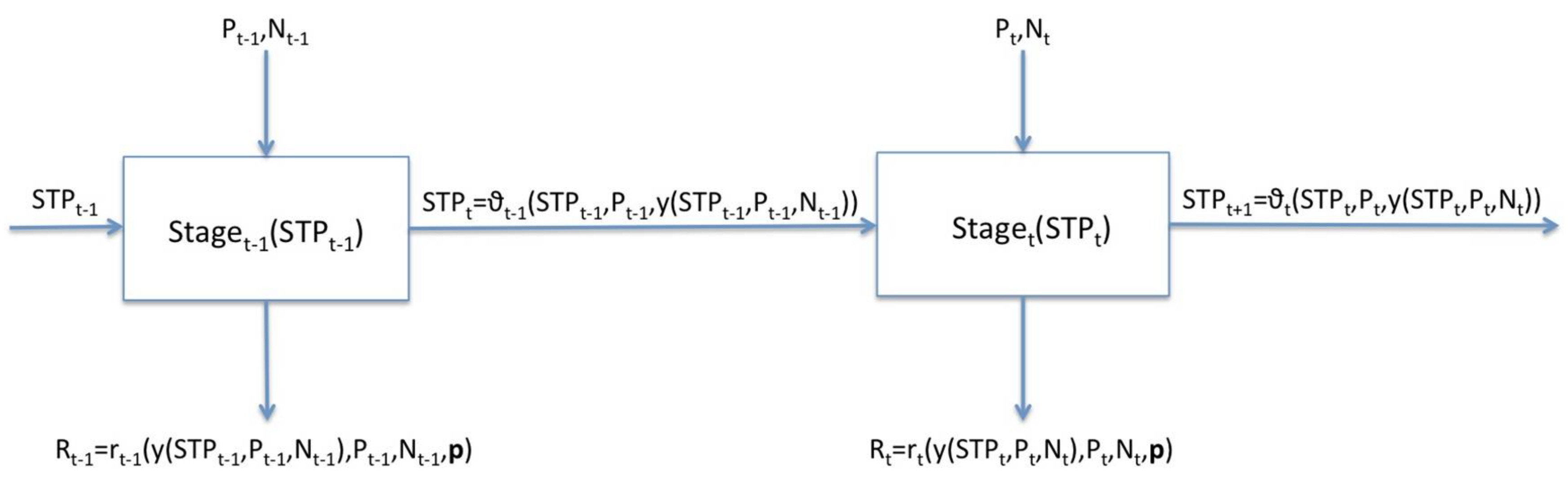
These findings were used to develop the conceptual farm-level dynamic decision model, where the planning horizon of the agricultural production, occurring on a representative field hectare, was divided into T stages at time (Figure 2). The length of a stage is one year. In each stage, the producer decides the amount of N and P fertilizers used. Each stage is characterized by a STP level, the state variable of the system. The system changes from one state at stage to another at the next stage, , as described by the transition function . The transition function is a function of the current state of the system (), the fertilization decisions made at that stage, and , and the resulting output, i.e., the current crop yield : = . At each stage, the decisions made and the state of the stage result in a stage return, , where is a stage return function, which is a function of the current output, input decisions, and fertilizer and crop prices (denoted by a vector ).
The data applied for the estimation of the yield response models included six separate datasets collected by Valkama et al. [9,12] that described the measurements from Finnish P and N fertilizer field experiments of cereals for clay and coarse-textured soils. The standardization of the separate datasets is shown in Appendix A1. Additional datasets for specifying the impact of STP on crop yield without added P fertilization were obtained from Saarela et al. [11], since the information regarding this relationship was limited in the data obtained from Valkama et al. [12]. Consequently, we were able to model the linkage between P response and STP, and the linkage between yield without added P and STP. However, the N fertilizer experiment datasets contained no information regarding the amount of N in the soil. Instead, the yields without added N were reported in the N datasets. Furthermore, the association between N response and the yields without added N was significantly negative (correlation = −0.63 (p-value = 2.35 × 10⁻⁸) for coarse soils and correlation = −0.49 (p-value = 0.00027) for clay soils). The datasets were initially unbalanced panel datasets, implying that the datasets contained multiple observations for each cross-section unit in the sample, but the time dimension was not the same for each individual experiment. However, the observations in the applied datasets were averaged over the experimental years. Therefore, the observations from longer experiments were more reliable, since these data were less affected by random variation attributable to weather-driven events [50]. Notably, the observations within the datasets were serially correlated, since multiple measurements were obtained from the same site. Moreover, for model validation, two independent datasets were gathered, including 28 short-term and long-term NPK fertilizer field experiments conducted in Finland between 1964 and 1988 at 10 sites on clay and coarse-textured soils. All the eight applied datasets are provided in the supplemental material.
2.2. Phase II: Model Development
In the applied datasets, the yield responses to individual nutrients were described as a relative increase in yield compared to the yield without the added nutrient. The Cobb−Douglas production function [51] is commonly used to describe such relationships. Our model specification resembled the Cobb−Douglas Mitschelich−Baule type production function [52] in that it included three multiplicative elements:
where
where denotes the crop yield (kg ha−1), is a particular fertilization experiment, denotes the yield without added P (kg ha−1), is a scaling factor for P fertilization, is a scaling factor for N fertilization, is a given nonlinear function specified by a certain structure for a model element , indicates an unknown parameter with subscript denoting a parameter number, indicates the model residual error, and denotes the yield without added N (kg ha−1). It is assumed that Equation (1) satisfies the typical properties of a production function [53]. The first element, defined by Equation (2), determines a yield without added P (kg ha−1) as a function of plant available soil P. The second element, defined by Equation (3), determines the yield response (%) to P fertilizer as a scaling factor that scales the first element up depending on the P application rate (kg P ha−1) and the STP level. The third element, defined by Equation (4), determines the yield response (%) to N fertilizer (kg N ha−1) as a scaling factor that scales the yield up or down depending on whether the N application rate is lower or higher than the average N rate in P experiments. The third model element is a decreasing function of yield without added N (kg ha−1). In model applications, was treated as a parameter rather than a variable due to the non-availability of a suitable transition function describing the N dynamics in the soil. The absence of a model component describing the N stock development is recognized as a model limitation. We hypothesized that a yield without added N must be lower than that without added P because typically N has a stronger effect on yields compared with P or STP [30,54]. Therefore, was fixed to a “reference-level” of 2/3 (2148 kg ha−1 and 2466 kg ha−1 for coarse-textured and clay soils, respectively).
We used the weighted nonlinear least squares method for separately estimating the parameters for the particular functional forms used for in Equations (2)–(4). We weighted the observations with the duration of the respective experiment. The heteroscedasticity and serial correlation of the data were considered by applying heteroscedasticity-and-autocorrelation-consistent (HAC) standard errors [55]. For the N fertilization data on clay soils, however, the application of HAC standard errors was insufficient to prevent the estimates from being almost perfectly correlated. Therefore, in this case, we applied nonlinear mixed-effect (nlme) modeling, where the unobserved site-specific characteristics were treated as random effects and the data were grouped by the experimental plots. Estimations were based on the maximum likelihood in this approach. The impacts of the random effects were assumed to be asymptotically normally distributed and zero on average. The residual error included two mutually independent and additively separable parts. These are a random effect for group , and the random residual for individual response of group is as follows: , where and . Consequently, Equation (4) takes the following form for clay soils: . Since the average expected yield is considered within the optimization and predictions, the site-specific random effects were set to their average expected level. More details about the estimation process can be obtained in Appendix A2.
Typically, multiple models can be fitted successfully into data [8,56]. Therefore, we examined several variations and combinations of commonly applied functional forms of in model elements in Equations (2)–(4) [35,57]. As a result of this process, we obtained a set of candidate models. We chose four or five models out of the numerous iteratively obtained alternatives for each model element in Equation (1) for both soil textures. We ranked the estimated models using the modified second order variant of Akaike information criteria (AIC) [36]. In addition, we calculated the relative likelihoods to quantitatively compare the models. We also performed a statistical goodness-of-fit analysis, as AIC is unable to indicate how well the models fit the data used for estimation [58]. In particular, the minimum requirement for a model performance is that the Nash−Sutcliffe efficiency (NSE), defined as the ratio between the residual variance and the measured data variance [59], must be positive. Following the recommendations of Moriasi et al. [60], we used NSE as an overall indicator of model efficiency instead of the index of agreement (IA) by Willmott [61], because IA clearly overestimated the model performance.
2.3. Phase III: Verification and Validation
We explored the model behavior via various simulations. We also used graphical comparison, statistical goodness-of-fit analysis, and standard statistical tests to compare the simulated versus observed data. We tested the normality of the residuals between observations and predictions using the Shapiro−Wilk normality test. We also estimated the following simple regression model:
where is the observed yield and is the simulated model prediction, to evaluate the linear relationship between predictions and observations. In this study, we tested the following composite hypothesis: H0: = 0 and = 1 [62,63]. Due to the serial correlation, following the suggestions of Marcus and Elias [63], HAC standard errors were again applied. Finally, we performed a paired t-test where the null hypothesis was that the mean of the observations is equal to the mean of the predictions, to quantify the differences between the observations and the predictions [62].
2.4. Phase IV: Formulation of the Dynamic System Model
To obtain the dynamic decision model (Figure 2), we coupled the estimated yield response models with the transition functions describing the soil P dynamics. We applied the following model [64]:
where indicates time (year), defines a transition from state to the next state , with as parameters, and indicates the P balance of the soil at time . The model of Uusitalo et al. [64] was developed for similar conditions to those estimated in this study. As such, the model required no calibration. We used the following model for the P balance [17]:
where and are parameters, and the term determines the P concentration of the crop yield. Thus, a P balance describes the difference between annually added P and removed P with the harvested yield, which is an increasing function of both and .
2.5. Phase V: Model Application for Economic Optimization
We formalized the economic optimization problem as a recursive finite horizon dynamic programming problem [65], where the objective is to maximize the net present value (NPV) of the discounted sum of the annual returns over the planning horizon by adjusting the control variables:
subject to
where is a discount factor, is a constant discount rate, is a state return function, is a constant price for yield, and denote constant prices for P and N, respectively, denotes an average expected yield at time (Equation (13) is an expectation of Equation (1) for a given ), denotes a scrap value [66], which approximates the following value of land after the production period: , and indicates the initial soil P level. This type of problem formulation is appropriate if we assume that the producers are risk-neutral, profit maximizers, and price takers. Furthermore, we assumed that farmers will own their farm for the decades ahead. Typically, farmers are interested in maximizing expected long-term profit if the farmer is a landowner and thus have a long-term planning horizon [67]. We evaluated the suitability of the certain functional form for economic optimization by examining whether the following requirements were satisfied: the optimal control trajectory must converge to a finite steady state where the optimal solution for each stage remains approximately the same, and the optimal steady-state fertilizer rates, STP levels, and the yields do not exceed the corresponding sample maximums.
2.6. Phase VI: Uncertainty and Sensitivity Analysis
We evaluated the sensitivity of the optimization results to the structural uncertainty by solving Equations (8)–(14) for different functions in constraint Equation (13) [8,57]. We also calculated the differences in NPV by simulating the best models for input vectors obtained from other model candidates (Appendix A3, Table A1) to approximate the potential economic losses resulting from incorrect decisions when selecting a yield response model [8]. The model combinations applied in structural uncertainty analysis are described in Appendix A4. Moreover, we examined the effects of parameter uncertainty on model outputs using Monte Carlo analysis. In the analysis, the probability distribution of all model parameters were assumed to asymptotically follow a normal distribution. We generated 10,000 values for each model parameter and computed the corresponding yields to obtain one realization for the yield distribution, which we described with the mean and the variance. To obtain the sampling distributions for the descriptive statistics of the yield distributions, we generated 10,000 realizations for the given statistic by looping the procedure. We also performed a sensitivity analysis to determine the sensitivity of the optimization results to the exogenous model parameters. We applied partial sensitivity analysis where the effect of each parameter on economic optimization results was examined while all the other parameters were held constant.
3. Results
3.1. Model Estimation
After estimating numerous different model formulations for each model element in Equations (2)–(4), by fitting various types of nonlinear functional forms for each dataset, and ranking the obtained model candidates using AIC (Appendix A3, Table A1), we obtained the explicit form for the Cobb−Douglas type yield response model for coarse soils and for clay soils, respectively, as follows:
where is the average expected yield, STP is the soil test phosphorus, P is the phosphorus fertilizer, N is the nitrogen fertilizer, and is a parameter with , indicating a model element, and indicates a parameter number in the given model element. Parameter denotes the minimum level of the scaling factor defining the P response. The numbers below Equations (15) and (16) refer to the model elements given in Equations (2)–(4). Hence, the first model element in Equations (15) and (16) defines the average expected yield without added P as a function of STP (recall Equation (2): ). The second model element in Equations (15) and (16) defines the average expected yield response to P fertilization as a function of P and STP (recall Equation (3): ). The third model element in Equations (15) and (16) defines the average expected yield response to N fertilization as a function of N and yield without added N (recall Equation (4): ). Table 1 shows the estimated parameters and the summary statistics for each model element of Equations (15) and (16). All the parameters were statistically significant at the 5% significance level.
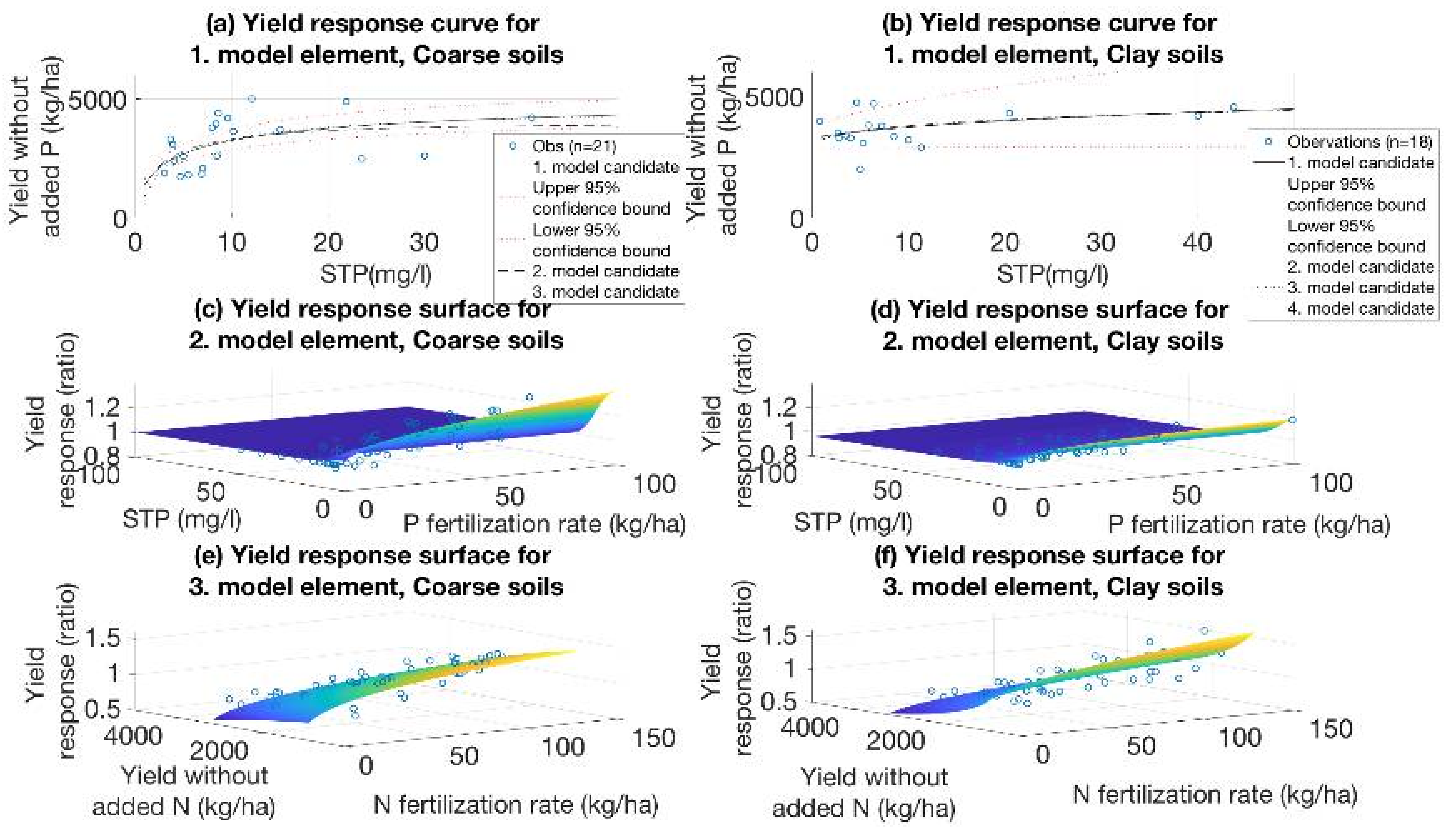
For both soil textures, the ability of the models to capture the observed variability in the data was highest for the N response models, indicating that the addition of the variable yield, without added N, corrects most of the omitted variable bias related to the omission of the soil N. In particular, the addition of site-specific random effects mitigated the omitted variable bias. The high predictive accuracy of the N response model for clay soil resulted from the fact that most of the variation could be explained by the random effects. The average value of the random effects was 0.0015 across the 15 groups and the associated standard deviation was 0.13, whereas the standard deviation of the residual errors was 0.088. However, the nlme approach was not applied to the other models since it reduces the generalizability of the models. This became apparent by the poorer fit to the validation data. Notably, the use of independent datasets for validation is known to be a convenient way to avoid the problem of overfitting [68]. The Nash–Sutcliffe efficiency (NSE) was also highest for the N response models for both soil textures (Table 2). In contrast, the discrepancy between observations and the model predictions was greatest for the model element describing the relationship between STP and yield without added P for both soil textures. The high prediction error was related to the relatively high variation in the dependent variable (yield) within the respective datasets, indicating that many other unobserved factors determining the variability in yields without added P, possibly more important than STP, exist.
3.2. Verification and Validation Results
Figure 3a,b show the simulated yield N-P-response surfaces for the fair STP class. The response surfaces are concave with respect to both nutrients. Moreover, the response surfaces for clay and coarse-textured soils were of the same order of magnitude, although for coarse soils, the observed P response (8.4% on average) was greater than that for clay soils (4.6% on average). For clay soils, in the other hand, the observed N response (74% on average) was greater than that for coarse soils (53% on average) (see footnotes for Tables S2 and S5 and for S3 and S6). Figure 3a,b also show that P fertilization does not affect the yield increases caused by N fertilization and vice versa. In this study, the yield responses of individual nutrients were estimated from the separate datasets; therefore, the interactions that are typically captured by the interaction term in polynomial function form could not be explicitly captured.
Figure 3c,d illustrate the yield response curves for various STP levels and show a non-monotonic yield response to STP for a certain range of the domain for substantial P fertilization applications. The non-monotonicity results from the yield-increasing effect of P fertilization (modeled by the second model element) is considerable for low STP levels, whereas the effect vanishes for higher STP levels (Appendix A3, Figure A1c,d). The yield in absolute terms, however, was an increasing function of STP (the relationship was modeled by the first model element). Therefore, the yield increased again for even higher STP levels. Thus, the interaction of the first and second model elements and the shapes of the respective response curves and surfaces (Appendix A3, Figure A1a–d) were a result of the non-monotonicity observed in Figure 3c,d.
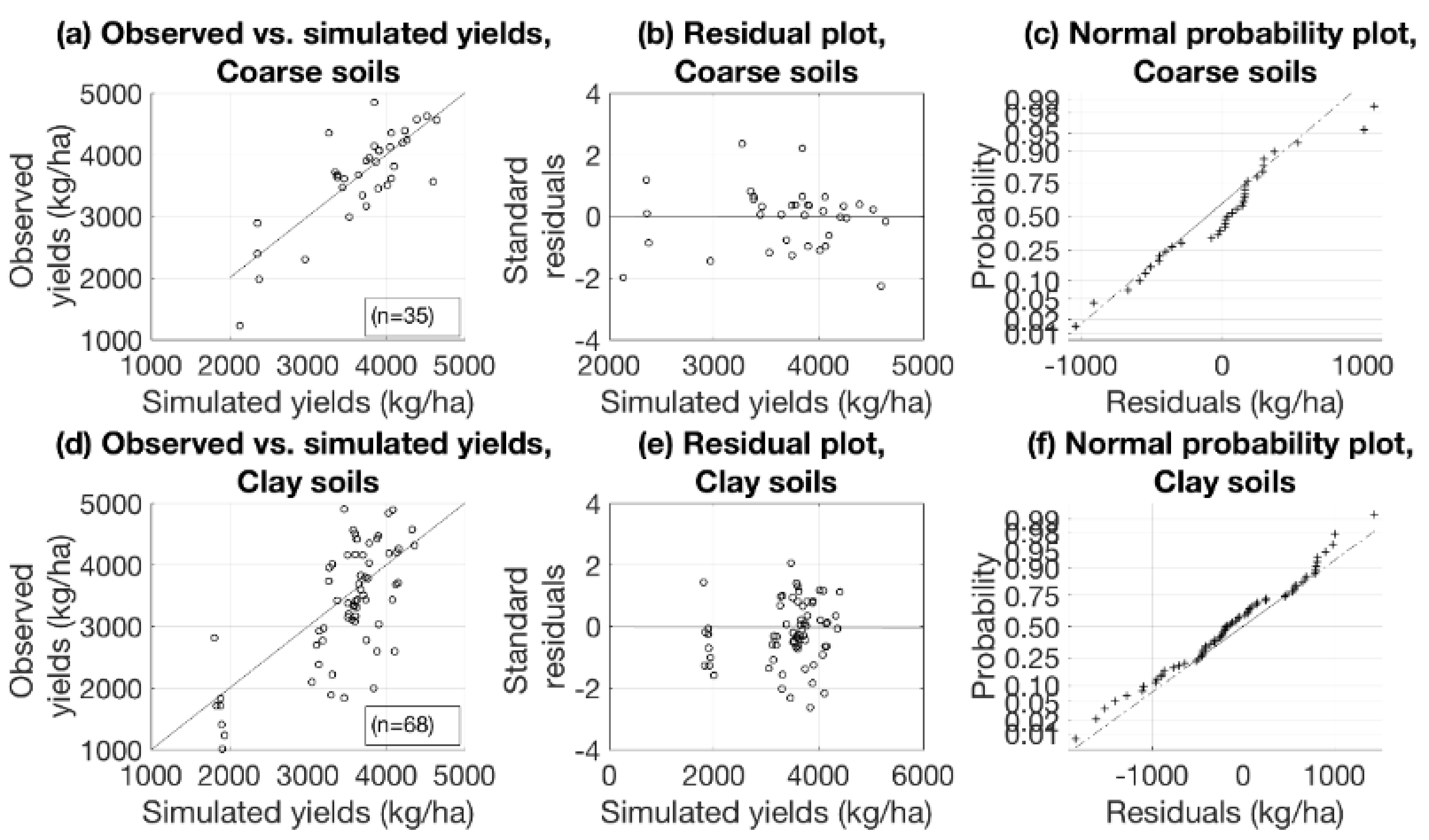
For both soil textures, the correlation between predicted and observed yield was reasonably high, suggesting that the model adequately represents the experimental results (Table 3). In addition, the relatively high NSE indicates that the variation in the observed yields was captured well, and the model simulation can be judged as “good” for coarse soils and “satisfactory” for clay soils [60]. The statistics measuring the prediction accuracy indicated that the model for coarse soils had a smaller prediction error than that for clay soils, which is mainly due to the greater amount of variation in yields in the clay soil data compared to that in the coarse soil data.
For both soils, the distribution of the residual errors was not significantly different from a normal distribution (Table 4). The estimation results of the simple regression described in Equation (5) showed that, for both soil textures, the parameter was nonsignificant at the 5% significance level, whereas the estimate for the -parameter was almost one and significant at the 5% significance level, indicating accurate predictive performance. The results of the paired t-test indicate that the mean of the observations was not significantly different from the mean of the predictions for either models, indicating that the absence of the interaction effect of P and N fertilization may be of minor importance for the performance of the models. This conclusion holds particularly well for the coarse-soils model.
For clay soils, more observations were overestimated than underestimated, demonstrated by the relatively high mean bias, which was expected because the average yield in the validation dataset for clay soils was only 3307 kg/ha (Table S8). However, the systematic bias was minor (Figure 4e). The normality of the residual errors appears in Figure 4c,f. Moreover, the distribution of the residual errors was more normal in clay soils, as suggested by the Shapiro−Wilk normality test.
3.3. Economically Optimal Nutrient Inputs and Uncertainty Analysis
For comparison, Table 5 shows the steady-state solutions obtained by solving the economic optimization problem by dynamic programming and by simulating the model using the present maximum permissible N and P rates denoted by the voluntary Finnish agri-environmental scheme. Applying rates equal to or below these maximum permissible rates is necessary for receiving the payments that provide compensation for additional or opportunity costs or both resulting from obeying environmentally friendly farming practices. The comparison shows that, for both soil textures, the economically optimal steady-state N rates were close to the maximum permissible N rates when the exemplary prices are valid. Instead, the economically optimal steady-state P rate was 36% higher on coarse soils and 58% lower on clay soils than for the maximum permissible P rates. Consequently, the steady-state STP level for economically optimal fertilizer rates was slightly higher for coarse soils and slightly lower for clay soils than the steady-state STP level for the fertilizer rates set at the maximum permissible level. Despite these differences, losses in annual profits and NPV were marginal in both cases. However, the chosen prices and the discount rate affected these results. The examination of the sensitivity of the optimization solution to the input costs, output price, and discount rate is shown in Appendix A4.
The statistics in Table 6 show that the average effect of the structural uncertainty is minor for both soil textures. The average economic loss of applying the “wrong” model, measured by the difference in NPV for the best model and any other model candidate, indicated by NPV (€ ha−1), is also minor. The relative (mean-scaled) effect of the structural uncertainty on model output was greater for coarse soils. Regardless, the relative cost of structural uncertainty was greater for clay soils.
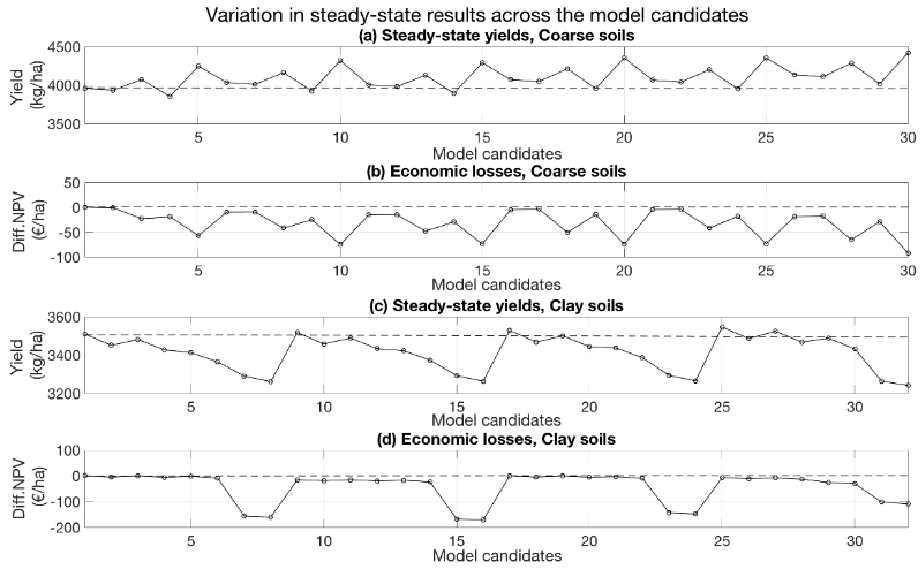
For coarse soils, most of the structural uncertainty effect was associated with the choice of the third model element (Figure 5a,b), which indicates that we were able to successfully fit function specifications, providing different response surfaces to the initial dataset. This can also be seen in Table 6, which shows that the relative effect (SD/Average) of the structural uncertainty was greater for optimal N fertilization (0.139) than for optimal P fertilization (0.07). Instead, for clay soils, the effect of structural uncertainty was mostly explained by the choice of the second model element (Figure 5c,d). Notably, Table 6 shows that, for clay soils, the relative effect of the structural uncertainty was greater for optimal P fertilization (0.41) than for optimal N fertilization (0.053). For both soil textures, the choice of the first model element had only a minor effect on the steady-state yield and NPV. However, the choice of the functional form affected the determination of the optimal steady-state yields (Figure 5a,c), and the incorrect choice may have economic consequences for the producer (Figure 5b,d).
The effect of parametric uncertainty on model output was greater for clay soils than for coarse soils (Table 7). For both soil textures, most parametric uncertainty stemmed from the third model element, the N response model. Moreover, the effect of parameter uncertainty on model output was greater than the effect of structural uncertainty. For coarse and clay soils the SD/Average ratios associated with the structural uncertainty were 0.037 and 0.027 for coarse and clay soils, respectively, whereas the corresponding ratios associated with the parametric uncertainty were 0.106 and 0.196 for coarse and clay soils, respectively.
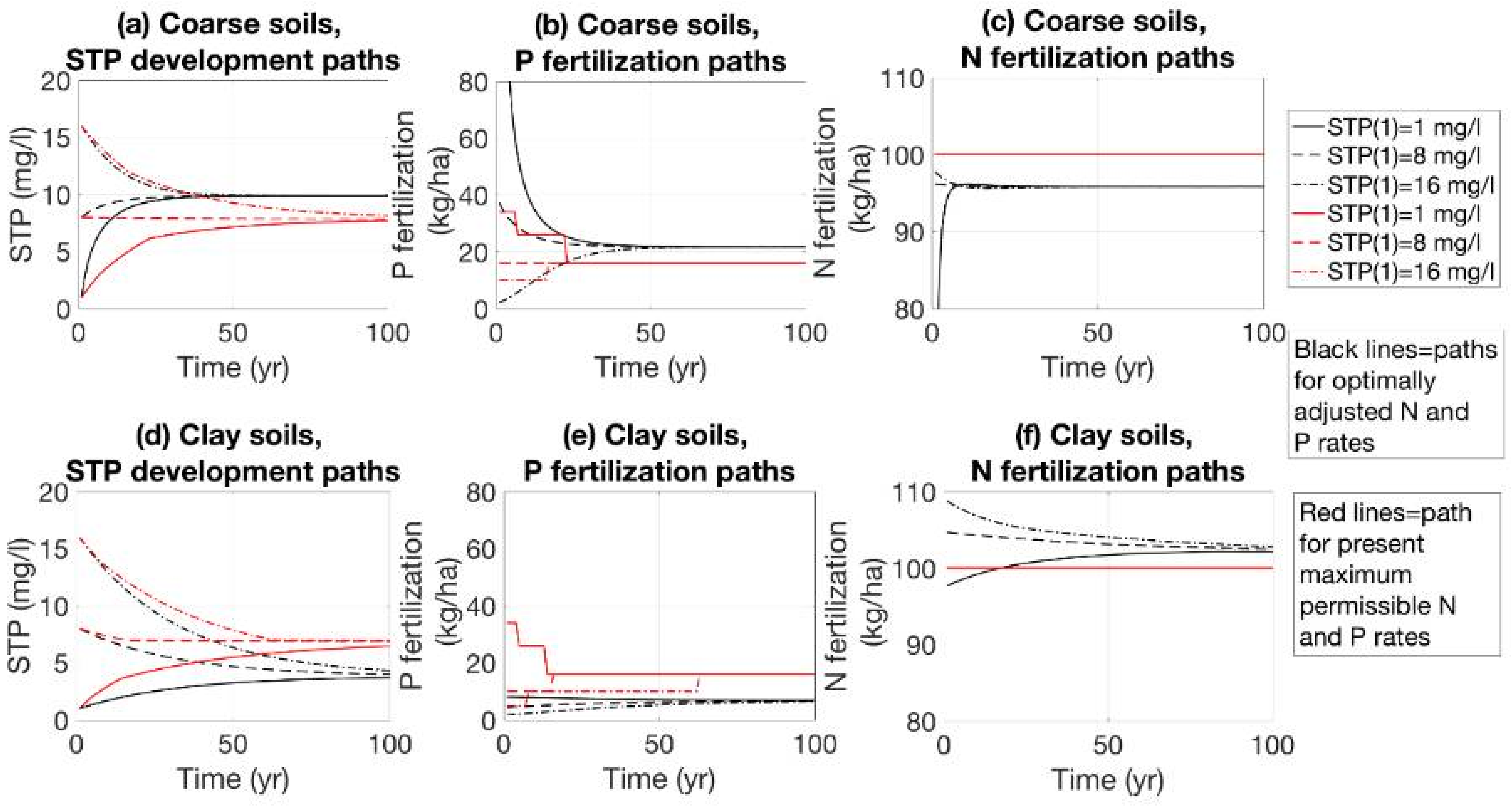
Lastly, we explored the effect of the initial STP level on optimization results using sensitivity analysis. The compared strategies were those where fertilization rates are adjusted to the initial STP levels by optimization and where the present maximum permissible rates of the voluntary agro-environmental scheme for each STP class are applied. When the initial STP level was below the steady-state level, applying a P rate above the steady-state level and a N rate below the steady-state level at the beginning of the planning horizon is optimal to rapidly achieve the steady state for STP (Figure 6). This resulted from the fact that, in the applied transition function for STP, the effect of N fertilization on STP development is negative:
Instead, when we differentiated the transition function with respect to P fertilization, we obtained the following condition:
In numerical applications, the effect of P on the development of STP is always positive (), since , [17], and . Conversely, when the initial STP level is above the steady-state level, there is no need for P fertilization for a long time. However, the STP level eventually declines below the steady-state level if no P fertilization is applied. To avoid this outcome, the optimal P fertilization rate thus increases steadily from zero to its steady-state level. Correspondingly, the optimal N rate is above the steady-state level at the beginning of the planning horizon and lowers to its steady-state level steadily. The convergence to the steady state was more gradual for clay soils than for coarse soils, since the N input is relatively more important for clay soils (Figure 6c,f).
When the present maximum permissible rates were applied, the path for STP development was similar to the path for optimally adjusted fertilization rates (Figure 6a,d). Additionally, the P fertilization paths for the two strategies resembled one another (Figure 6b,e). For coarse soils, the optimally adjusted P fertilization rate for the poor STP class was considerably higher than that of the maximum permissible rate strategy. For clay soils, the P fertilization rates for all STP classes were higher for the maximum permissible rate strategy than those for the optimally adjusted rates strategy. The differences between the management strategies were greatest for the first 10 years of the planning horizon. The difference between the N fertilization paths was minor in absolute terms between the two management strategies for both soil textures, although the optimally adjusted N fertilization rates adjusted slowly to the steady state for clay soils (Figure 6c,f).
The initial STP had a relatively minor effect on the NPV for clay soils, with the difference between very low and high STP being approximately 1000€, compared to coarse soils where the difference was approximately 3000€ (Figure 7). Moreover, the application of the present maximum permissible rates led only to small economic losses.
4. Discussion
An advantage of using the existing extensive experimental data, available separately for N and P responses, is that we were able to avoid the multicollinearity problem. Another strength is that applying existing data is cheaper than conducting new field experiments [70]. A disadvantage is that possible interactions in the joint effect of N and P fertilizer inputs were neglected due to the use of data from separate experiments for the two nutrients [38,39,71]. Conversely, since the estimated models performed relatively well against the independent NPK fertilizer experimental data used for validation, the neglected interaction might be of less importance. Furthermore, the structure of the model and the modeling process described in this study can, after calibration and validation, generally be applied for any region, given that the required data are available.
Our results about the effect of the initial STP level on the optimal fertilization management showed that applying P on soils characterized by high STP levels according to the present interpretation is not practical, whereas for soils characterized by low STP levels, substantial P rates are economically justified. Similar findings were reported by Cox [72] and Valkama et al. [12]. Maintaining fair or satisfactory STP levels has also been shown to require surplus P fertilization [15,29,73]. In some cases, accumulating and maintaining a certain level of STP to obtain optimal crop yields may be profitable [44,74]. According to our results, maintaining a fair STP level on both coarse-textured and clay soils was profitable. However, for coarse soils, this required higher P fertilizer inputs than clay soils, and the actual STP value was higher. This result shows the general effect of soil texture on the relation of P availability and STP for the examined specific region, and the generalization of the result requires exploration in other climatic regions. Thus, on coarse soils, the optimal fertilization strategy is more or less a so-called “build-up and maintenance” approach with a focus on the available amount of a nutrient in the soil. On clay soils, the optimal fertilization strategy follows more a “sufficiency” approach with a focus on the plant needs [2,44]. For N fertilization, the rate of convergence to the steady state was rapid for coarse soils and gradual for clay soils, reflecting the relative importance of the nutrients. Somewhat similar findings were obtained by Lambert et al. [18]. Thus, based on our results, the optimal steady-state fertilization rates and STP levels depend on the soil texture, among many other factors not included in the models. This result is consistent with suggestions provided by Syers et al. [44] and Reetz [2].
The developed models can be used to estimate the compensation farmers should be given for lowering the fertilization rates below the economically optimal rates. Our optimization results indicate that, although the present maximum permissible fertilization rates of the voluntary agro-environment scheme were somewhat different compared with the economically optimal fertilization rates determined by the models, the economic losses resulting from applying the maximum permissible rates were low. These results indicate that the present maximum fertilization rates applied in Finland successfully consider the effect of soil P dynamic feedback on optimal fertilization rates. For such cases, the compensation that farmers receive from applying fertilization rates that are different than the economically optimal rates could be minimal.
Previous studies showed that imperfect information regarding the model structure is often the main source of uncertainty associated with the model output [56,75]. Our results of the uncertainty analysis showed the opposite: the effect of the parametric uncertainty on model output was greater for both soil textures than the effect of the structural uncertainty. However, we examined only the structural uncertainty for the mathematical formulations and ignored the structural uncertainty caused by the choice of processes included in the model. The effect of functional forms on optimal fertilization rates have often been shown to be significant [8,76,77]. Our results for the effect of structural uncertainty on optimization results showed that the effect of functional form choice on optimal fertilizer rates was minor. Thus, via iterative elimination of plausible functional forms, by dropping the less suitable functional forms from further consideration in multiple phases, we efficiently reduced the effects of structural uncertainty on model output and optimal input decisions.
The results of the parametric uncertainty analysis showed that the parameter uncertainty had a greater impact on model output for clay soil models compared with coarse soil models. The impact of parametric uncertainty for clay soil models was associated with the greater variation in yield response to fertilization inputs within the initial data. This positive association between noisy data and model uncertainty has been recognized in previous literature [78,79,80].
Modeling exercises help detect areas where knowledge and data are scarce [81]. We identified several issues that need additional research. First, given the large variation in observed yields without added P, particularly for clay soils, more long-term data on the relationship between yield without added P and STP, and the critical factors affecting P supply from soil to plants that may not be covered by STP measurements only, are needed [82,83]. Secondly, more data and research are needed about the dynamics between soil N and soil organic matter (SOM), and the effect of these variables on crop yield. The weak association between SOM and a yield response was ignored in this study [9]. Instead, the N status in the soil is quite volatile [84,85,86]. Due to the data limitations and to consider the absence of soil N, our approach was to include a yield without added N into a model as an independent variable. Consequently, the N response models performed well against the initial N experimental data. Nevertheless, we recognized the absence of the N transition function from the economic model as a model limitation. To fully capture the dynamic behavior of the system, the soil N should be included in the economic model as a state variable. Hence, a natural extension for this study is the estimation of the transition function for N and the coupling of the transition function with the economic model. This extension, however, can be included in the model only once the data limitations are overcome. Moreover, the economic model could be expanded by introducing stochastic weather-related variables. Agriculture is strongly influenced by seasonal, weather-related, and climate-related uncertainty [87,88,89]. Annual variation in crop yields is often explained better with annual weather-related variation in production conditions than with variation in fertilizer application rates [12,30,90]. Nevertheless, when considering the long-term management of a farm, focusing on average expected yield is reasonable. Last, the explicit examination of the leaching potential remains a subject for further studies, since this would require coupling the system models with appropriate leaching functions for N and P.
5. Conclusions
The validation results suggest that the key relationships determining the crop responses were captured by the Cobb−Douglas type model specification consisting of multiplicative elements. The estimated models can be extended to assess the impacts of alternative management prescriptions and agricultural policies on the economic surplus of crop cultivation. This information may help improve long-term fertilization management plans. On coarse-textured soils, the optimal fertilization strategy can be described as build-up and maintenance, whereas on clay soils the optimal fertilization strategy is in line with the sufficiency rule of thumb. However, to fully capture the nutrient dynamics in bio-economic modeling, further research is required. Modeling approaches based on iterative elimination of plausible functional forms were efficient at reducing the effects of structural uncertainty on model output and on optimal input decisions.
Supplementary Materials
The following are available online at https://www.mdpi.com/2073-4395/8/4/41/s1, Table S1: Dataset for the first model element for coarse soils, Table S2: Dataset for the second model element for coarse soils. STP was measured at the beginning of experiments from the control (without added P), Table S3: Dataset for the third model element for coarse soils, Table S4: Dataset for the first model element for clay soils, Table S5: Dataset for the second model element for clay soils, Table S6: Dataset for the third model element for clay soils, Table S7: Validation dataset for coarse soils, Table S8, Validation dataset for clay soils.
Acknowledgments
This work resulted from the BONUS BALTICAPP project and was supported by BONUS (Art 185), funded jointly by the EU and Academy of Finland. We would like to thank Antti Iho, Antonios Rezitis, Timo Sipiläinen, Stefan Bäckman and Risto Uusitalo for their constructive comments. All remaining errors are the authors’ responsibility.
Author Contributions
The original research idea was developed by Kari Hyytiainen and Matti Sihvonen. The study was also planned by Kari Hyytiainen and Matti Sihvonen. Kari Hyytiainen was also responsible for commenting and writing the manuscript. Matti Sihvonen was mainly responsible for writing the manuscript, carrying-out the coding and all the numerical estimations and optimization calculations, formulating the economic optimization framework, producing the results, and gathering the datasets used for model validation. Elena Valkama and Eila Turtola were responsible for providing the datasets used for the estimation of nitrogen and phosphorus yield response models. Elena Valkama and Eila Turtola also participated in writing and commenting the manuscript.
Conflicts of Interest
The authors declare no conflict of interest.
Appendix A
Appendix A.1. Standardization of the Separate Datasets
The standardization of the separate datasets proceeded according to the following steps. First, we defined the weighted average N fertilization rate applied in P fertilization experiments as a reference N rate (kg/ha) and labeled it . This rate was approximately 70 and 95 kg/ha for coarse and clay soils, respectively. We determined the yield response in a given experiment , corresponding to the reference N rate, with the following relationship:
where is the yield response observed in N-experiment corresponding to and is the hypothetical yield response obtained by applying the reference amount of N fertilization in this given experiment. Third, we used the average of the calculated yield responses corresponding to a reference N fertilization rate (), and we divided every yield response observed in the N experiment data by this value:
where is the reference N-scaled yield response for N fertilization in experiment . Thus, the N dataset was mean-scaled with the hypothetical average N response, corresponding to the average N rate applied in P experiments.
However, the N fertilization experiment data had to be scaled with respect to the reference yield without added N (), which was set as two-thirds of the average yields without added P. A 2:3 ratio was considered as a scaling parameter to be calibrated, labeled by . Thus, , where is an average yield without added P and is a scaling parameter. We then repeated the second and third steps for the reference yield without added N:
where is the yield response observed in N-experiment corresponding to and is the hypothetical yield response obtained if the yield without added N would have been equal to the reference yield without added N in the given experiment. Next, we used the average of the calculated yield responses corresponding to a reference yield without added N () and divided every reference N-scaled yield response observed in the N experiment data by this value:
where is the scaling factor for the yield response to N fertilization in experiment . These scaled data were used for the estimation of the third model element.
Appendix A.2. Estimating the Yield Response Models
The yield response models were estimated by applying the weighted nonlinear least squares (WNLS) method, where the numerical (iterative) minimization is used to minimize the weighted residual sum of squares (RSS) as follows:
where is an observation in a particular field experiment, is the weight of the observation , is an observed dependent variable, denotes an observed explanatory variable, is a parameter to minimize the RSS, and is a nonlinear functional form. Since no closed-form expression for exists, a numerical optimization procedure was used to compute . In this optimization procedure, the RSS was calculated iteratively for different parameter values, which were determined based on the data, the model, and the current parameter values, until the predetermined stopping criteria was satisfied, meaning an optimum was approximately reached. The decrease in RSS value obtained by changing the parameter values was so small that the iterative process was stopped, meaning the parameter values converged. The iterative optimization procedure required adequate starting values for the convergence. Further, fitting many functional forms to data with almost identical success is functionally possible. This was the case for our datasets. Therefore, we tried many different functional forms for .
Before fitting any functional form, the first step was always to graphically examine the shape of the distribution of the observations in a given dataset. This preliminary examination provided a glimpse of the possible functional form that could be used to describe the data and the range of the possible starting values for the parameters. When a particular functional form was chosen and fitted to data, we graphically explored the shape of the resulting yield curve or surface first. At this step, particular attention was paid to the concavity and convergence of the model. These properties are essential to optimize the designed models. After visual exploration, we examined the associated residuals and the goodness-of-fit statistics, comparing the model simulations and observations. After graphical and statistical exploration, the functional form was used in dynamic economic optimization and simulations. If the function form performed according to intuition and the general findings from the literature in optimization and simulation applications, the functional form was included in the set of candidate models, which were eventually ranked using AIC.
We applied bootstrapping for the first model element for clay soils. Bootstrapping was applied because the dataset was so small that bootstrapped standard errors and parameter estimates were considered more liable than the small sample WNLS estimates. During bootstrapping, we mimicked the repetition of an experiment by resampling the dataset B times with repetition. For each B dataset, the WNLS was applied:
where is a particular bootstrap sample. The bootstrap estimate was obtained as an average of the obtained estimates:
and the variance-covariance matrix of was estimated by the empirical variance–covariance matrix of :
For nonlinear mixed effect models, which is the third model element for clay soil models, . The likelihood method was applied for estimation instead of the least squares method. Using this method, we estimated the parameter values for by maximizing the likelihood of the observations :
where is the conditional density of the observations given the random effects, and is the density of the individual parameters of plot . Since is nonlinear, the likelihood was approximated numerically. Once the numerical approximation of the likelihood was obtained, the resulting likelihood was maximized by applying the standard quasi-Newton minimization algorithm.
All final estimations were performed with Rstudio software, using nlstools and nlme packages. A preliminary visual exploration of the yield response curves and surfaces and preliminary fits were performed using MATLAB software. All starting values for WNLS and nlme estimations were obtained by first fitting the model with the MATLAB Curve Fitting toolbox. In addition, all optimization and simulation applications were performed with MATLAB.
Appendix A.3. Estimated Models and the Yield Response Curves and Surfaces
Table A1 shows the estimated models for each model element in the yield response models for coarse and clay soils. The model candidates are ranked from best to worst by Akaike information criteria (AIC).

Table A1.
The estimated models and the summary of the model ranking results for coarse and clay soils †.
Table A1.
The estimated models and the summary of the model ranking results for coarse and clay soils †.
| Soil Texture, Model Element ‡ | Model Structure § | |||||
|---|---|---|---|---|---|---|
| Coarse 1. Model element | 20.26 × 10⁶ | 317.0 | 0.00 | 0.42 | 1 | |
| 21.63 × 10⁶ | 318.5 | 1.51 | 0.20 | 2.13 | ||
| 20.06 × 10⁶ | 319.2 | 2.18 | 0.14 | 2.97 | ||
| 20.19 × 10⁶ | 319.4 | 2.34 | 0.13 | 3.22 | ||
| 20.39 × 10⁶ | 319.6 | 2.56 | 0.12 | 3.59 | ||
| 2. Model element | 0.335 | −344.5 | 0.00 | 0.54 | 1 | |
| 0.3315 | −343.0 | 1.51 | 0.25 | 2.12 | ||
| 0.3515 | −341.3 | 3.16 | 0.11 | 4.86 | ||
| 0.3532 | −341.0 | 3.49 | 0.09 | 5.73 | ||
| 3. Model element | 0.4828 | −300.5 | 0.00 | 0.27 | 1 | |
| 0.4836 | −300.4 | 0.10 | 0.26 | 1.05 | ||
| 0.4882 | −299.8 | 0.70 | 0.19 | 1.42 | ||
| 0.4920 | −299.3 | 1.20 | 0.15 | 1.82 | ||
| 0.4416 | −299.0 | 1.48 | 0.13 | 2.09 | ||
| Clay 1. Model element | 7.16 × 10⁶ | 236.8 | 0.00 | 0.29 | 1 | |
| 7.22 × 10⁶ | 236.9 | 0.06 | 0.28 | 1.03 | ||
| 7.23 × 10⁶ | 237.0 | 0.22 | 0.26 | 1.12 | ||
| 7.52 × 10⁶ | 237.8 | 0.95 | 0.18 | 1.61 | ||
| 2. Model element | 0.0698 | −264.5 | 0.00 | 0.34 | 1 | |
| 0.0711 | −263.7 | 0.78 | 0.23 | 1.476 | ||
| 0.0720 | −263.2 | 1.28 | 0.18 | 1.90 | ||
| 0.0684 | −263.0 | 1.49 | 0.16 | 2.110 | ||
| 0.0669 | −261.5 | 2.98 | 0.08 | 4.446 | ||
| 3. Model element | 0.2945 | −250.3 | 0.00 | 0.58 | 1 | |
| 0.3041 | −248.7 | 1.61 | 0.26 | 2.239 | ||
| 0.3163 | −246.8 | 3.57 | 0.10 | 5.96 | ||
| 0.3067 | −246.0 | 4.36 | 0.07 | 8.826 |
† RSS is the sum of squared residuals, AICc is the second order variant of Akaike’s information criteria, Δ is the AIC difference, is the Akaike’s weight, and is the evidence ratio between the best model (1) and another model j, and the parameter is the minimum observation for yield response (0.96). ‡ The 1. Model element refers to Equation (2) in the main text describing the association between soil test P (STP) and yield without added P (), 2. Model element refers to Equation (3) in the main text describing the yield response to P fertilization (), and the 3. Model element refers to Equation (4) in the main text describing the yield response to N fertilization (). § indicates expected average yield without added P, STP indicates soil test P, indicates the scaling factor for the average expected P response, indicates the scaling factor for the average expected N response, and indicates the yield without added N.
The representative yield response curves and surfaces and observed data points are shown in Figure A1. Figure A1a,b illustrate the yield response curves for the estimated STP response models. The response curves provided by the different models were almost identical for clay soils (Figure A1b). For coarse soils, the response curves were also almost identical for STP levels below 20 mg/L. After this threshold, the curves started to separate (Figure A1a). For the observed STP levels, all response curves provided by the different models were within the 95% confidence bounds of the best model candidates. Additionally, for coarse soils, the yield without added P sharply increased as STP increased when the STP level ranged from the poor to fair STP class. Instead, for clay soils, the yield without added P increased smoothly for higher STP levels. Figure A1c,d illustrate the associated predictive response surfaces for estimated best P response models. The yield response to P fertilization was observed only for STP classes ranging from poor to fair, whereas the response vanished rapidly for higher STP levels. The maximum P response was considerably higher for coarse soils than clay soils, indicating that the P fertilizer is a relatively more important input for coarse soils. Furthermore, the surface converged faster to its maximum plateau on clay soils when the P rate increased. Figure A1e,f illustrate the N response surfaces for the estimated models predicting lower yield responses to N fertilization for higher yields without added N. The maximum response to N fertilization was higher for clay soils, indicating that N fertilizer is a relatively more important input for clay soils. In addition, the coarse soil models converged to the maximum plateau for lower N rates. The illustrated models were the best model candidates.
Appendix A.4. Model Combinations Applied in Analysis of the Structural Uncertainty
The set of candidate models examined by analyzing the structural uncertainty would have been too large if all model combinations were considered. Therefore, we examined only the models for which the evidence ratio was less than three. For the coarse soils, there were three candidates for the first model element, two candidates for the second model element, and five candidates for the third model element, for a total of 30 models. For clay soils, there were four candidates for the first model element, four candidates for the second model element, and two candidates for the third model element, for 32 models in total.
Figure A1.
The data points and STP response curves for (a) coarse and (b) clay soils. The P response surfaces for (c) coarse and (d) clay soils, and the N response surfaces for (e) coarse and (f) clay soils provided by the best candidate models. For the third model element for clay soils, the random effects were set to their expected zero level.

Appendix A.5. Sensitivity Analysis Results
The results of the sensitivity analysis of the optimization for the economic parameters of the model, namely the prices for barley, fertilizer inputs, and the discount rate, were examined using partial sensitivity analysis. Table A2 shows the results of the sensitivity analysis. The P price had a considerable effect on optimal P fertilization, whereas it had a relatively minor effect on optimal N fertilization. Since the N fertilization was a relatively more important factor in determining the annual yield than P fertilization, the effect of the P price on optimal annual yields was relatively minor. Moreover, for every variable, the higher the P price, the lower the absolute amount of the variable, which would suggest that P and N are not easily substituted by one another. Both inputs are important factors for production. The P price had a greater effect on P fertilization for clay soils than for coarse soils. Instead, the effect on N fertilization and annual yield was greater for coarse soils. These results indicate that the P fertilization is a relatively more important factor for production with coarse soils than with clay soils. The N price had a considerable effect on the optimal N fertilization rate for both soil textures. As a result, the annual yields were considerably affected by N price. Moreover, the effect was similar for all variables: the higher the N price, the lower the optimal level of the variable. Because the N fertilization was a relatively more important factor for production for clay soils than for coarse soils, the effect of N price was more substantial for clay soils. The barley price also had a considerable effect on optimal fertilization rates. Furthermore, the effect of barley yield price on yield was greater for clay soils than for coarse soils, indicating greater elasticity in the yield price for clay soils.
Conversely, the effect of a discount rate was relatively minor compared with the other examined parameters. The higher the discount rate, the lower the optimal P fertilization rate for both soil textures. Instead, the optimal N fertilization rate was a decreasing function of the discount rate on coarse soils, whereas the optimal N fertilization rate was an increasing function of the discount rate on clay soils. This results from the fact that N fertilization was a more important factor for production on clay soils. Therefore, on clay soils, compensating for the marginal decrease in P applications caused by the increased discount rate by increasing the N fertilization rate is optimal. For coarse soils, the P fertilizer was a more important factor for production, so the reduction in P fertilization cannot be compensated by increasing applications of N.
Table A2.
The sensitivity of the steady-state N and P fertilizer rates and yields to the economic parameters of the model.
Table A2.
The sensitivity of the steady-state N and P fertilizer rates and yields to the economic parameters of the model.
| Parameter | Value | Steady-State P Rate | Steady-State N Rate | Steady-State Yield | |||
|---|---|---|---|---|---|---|---|
| Coarse Soils | Clays Soils | Coarse Soils | Clay Soils | Coarse Soils | Clay Soils | ||
| P price (€/kg) | 1 | 27.9 | 13 | 101.8 | 108.6 | 4123 | 3644 |
| 1.99 (baseline) | 21.7 | 6.78 | 95.8 | 102.4 | 3959 | 3509 | |
| 3 | 15.7 | 4.06 | 87.5 | 98.4 | 3699 | 3416 | |
| N price (€/kg) | 0.5 | 25 | 10.5 | 207 | 344.6 | 4635 | 4868 |
| 0.91 (baseline) | 21.7 | 6.78 | 95.8 | 102.5 | 3959 | 3509 | |
| 2 | 17.6 | 4.57 | 32.1 | 20.9 | 3183 | 2626 | |
| Barley price (€/kg) | 0.06 | 5.79 | 1.78 | 28.5 | 23.8 | 2693 | 2600 |
| 0.12 (baseline) | 21.75 | 6.78 | 95.8 | 102.4 | 3959 | 3509 | |
| 0.24 | 31.17 | 19.25 | 244.8 | 443.2 | 4898 | 5387 | |
| Discount rate (%) | 1 | 24.37 | 8.1 | 97.1 | 102.3 | 4029 | 3526 |
| 3.5 (baseline) | 21.75 | 6.78 | 95.8 | 102.4 | 3959 | 3509 | |
| 6 | 19.85 | 6.41 | 94.9 | 102.6 | 3897 | 3504 | |
References
- Snyder, C.S.; Bruulsem, W.T. Nutrient Use Efficiency and Effectiveness in North America: Indices of Agronomic and Environmental Benefit; International Plant Nutrition Institute: Peachtree Corners, GA, USA, 2007. [Google Scholar]
- Reetz, H.F., Jr. Fertilizers and their Efficient Use; International Fertilizer Industry Association (IFA): Paris, France, 2016; p. 114. [Google Scholar]
- Kang, Y.; Khan, S.; Ma, X. Climate change impacts on crop yield, crop water productivity and food security—A review. Prog. Nat. Sci. 2009, 19, 1665–1674. [Google Scholar] [CrossRef]
- Asseng, S.; Ewert, F.; Rosenzweig, C.; Jones, J.W.; Hatfield, J.L.; Ruane, A.C. Uncertainty in simulating wheat yields under climate change. Nat. Clim. Chang. 2013, 3, 827–832. [Google Scholar] [CrossRef]
- Popp, A.; Calvin, K.; Fujimori, S.; Havlik, P.; Humpenöder, F.; Stehfest, E.; Bodirskyah, B.L.; Dietricha, J.; Doelmanne, J.C.; Gusti, M.; et al. Land-use futures in the shared socio-economic pathways. Glob. Environ. Chang. 2017, 42, 331–345. [Google Scholar] [CrossRef]
- Gilbert, N. The disappearing nutrient. Nature 2009, 461, 716–718. [Google Scholar] [CrossRef] [PubMed]
- Bock, B.R.; Sikora, F.J. Modified-Quadratic/Plateau Model for Describing Plant Responses to Fertilizer. Soil Sci. Soc. Am. J. 1990, 54, 1784–1789. [Google Scholar] [CrossRef]
- Cerrato, M.E.; Blackmer, A.M. Comparison of models for describing corn yield response to nitrogen fertilizer. Agron. J. 1990, 82, 138–143. [Google Scholar] [CrossRef]
- Valkama, E.; Salo, T.; Esala, M. Nitrogen balances and yields of spring cereals as affected by nitrogen fertilization in northern conditions: A meta-analysis. Agric. Ecosyst. Environ. 2013, 164, 1–13. [Google Scholar] [CrossRef]
- Judel, G.K.; Gebauer, W.G.; Mengel, K. Yield response and availability of various phosphate fertilizer types as estimated by EUF. Plant Soil 1985, 83, 107–115. [Google Scholar] [CrossRef]
- Saarela, I.; Järvi, A.; Hakkola, H.; Rinne, K. Fosforilannoituksen Porraskokeet 1977–1994; Vuosittain Annetun Fosforimäärän Vaikutus Maan Viljavuuteen ja Peltokasvien Satoon Monivuotisissa Kenttäkokeissa. Maatalouden Tutkimuskeskus Tiedote 16/95; Maatalouden Tutkimuskeskus: Jokioinen, Finland, 1995. [Google Scholar]
- Valkama, E.; Uusitalo, R.; Turtola, E. Yield response models to phosphorus application: A research synthesis of Finnish field trials to optimize fertilizer P use of cereals. Nutr. Cycl. Agroecosyst. 2011, 91, 1–15. [Google Scholar] [CrossRef] [Green Version]
- Yajragupta, Y.; Halley, L.E.; Melsted, S.W. Correlation of phosphorus soil test values with rice yields in Thailand. Soil Sei Soe. Am. Proe. 1963, 27, 395–398. [Google Scholar] [CrossRef]
- Analogides, D.; Rendig, V.V. Functional Relationships between Yield Response and Soil Phosphorus Supply, Choice of the independent variable. Plant Soil 1972, 37, 545–559. [Google Scholar] [CrossRef]
- Dodd, J.R.; Mallarino, A.P. Soil-test Phosphorus and Crop Grain Yield Responses to Long-Term Phosphorus Fertilization for Crop-Soybean Rotations. Soil Sci. Soc. Am. J. 2005, 69, 1118–1128. [Google Scholar] [CrossRef]
- Kennedy, J.O.S.; Whan, I.F.; Jackson, R.; Dillon, J.L. Optimal fertilizer carry-over and crop recycling policies for a tropical grain crop. Aust. J. Agric. Econ. 1973, 147, 104–113. [Google Scholar]
- Iho, A.; Laukkanen, M. Precision phosphorus management and agricultural phosphorus loading. Ecol. Econ. 2012, 77, 91–102. [Google Scholar] [CrossRef]
- Lambert, D.M.; Lowenberg-DeBoer, J.; Malzer, G. Managing phosphorus soil dynamics over space and time. Agric. Econ. 2007, 37, 43–53. [Google Scholar] [CrossRef]
- Hansen, S.; Jensen, H.E.; Nielsen, N.E.; Svendsen, H. DAISY: A Soil Plant System Model; Danish Simulation Model for Transformation and Transport of Energy and Matter in the Soil-Plant-Atmosphere System; National Agency for Environmental Protection: Copenhagen, Denmark, 1990.
- Eckersten, H.; Jansson, P.-E.; Johnsson, H. SOILN Model–User’s Manual, 2nd ed.; Division of Agricultural Hydrotechnics Communications, Department of Soil Sciences, Swedish University of Agricultural Sciences: Uppsala, Sweden, 1994; p. 58. [Google Scholar]
- Keating, B.A.; Carberry, P.S.; Hammer, G.L.; Probert, M.E.; Robertson, M.J.; Holzworth, D. An overview of APSIM, a model designed for farming systems simulation. Eur. J. Agron. 2003, 18, 267–288. [Google Scholar] [CrossRef]
- Strauss, F.; Schmid, E.; Moltchanova, E.; Formayer, H.; Wang, X. Modeling climate change and biophysical impacts of crop production in the Austrian Marchfeld Region. Clim. Chang. 2012, 111, 641–664. [Google Scholar] [CrossRef]
- Van der Velde, M.; Folberth, C.; Balkovič, J.; Ciais, P.; Fritz, S.; Janssens, I.A. African crop yield reductions due to increasingly unbalanced Nitrogen and Phosphorus consumption. Glob. Chang. Biol. 2014, 20, 1278–1288. [Google Scholar] [CrossRef] [PubMed]
- Dzotsi, K.A.; Jones, J.W.; Adiku, S.G.K.; Naab, J.B.; Singh, U.; Porter, C.H.; Gijsman, A.J. Modeling soil and plant phosphorus within DSSAT. Ecol. Model. 2010, 211, 2839–2849. [Google Scholar] [CrossRef]
- Cichota, R.; Snow, V.O. Estimating nutrient loss to waterways—An overview of models of relevance to New Zealand pastoral farms. N. Z. J. Agric. Res. 2009, 52, 239–260. [Google Scholar] [CrossRef]
- Bolland, M.D.A.; Allen, D.G.; Barroe, N.J. Sorption of Phosphorus by Soils: How It Is Measured in Western Australia; Bulletin 4591; Department of Agriculture and Food: Kensington, Australia, 2003; p. 32.
- Li, X.; Coble, K.H.; Tack, J.B.; Barnett, B.J. Estimating Site-Specific Crop Yield Response using Varying Coefficient Models. Selected. In Proceedings of the 2016 Agricultural & Applied Economics Association Annual Meeting, Boston, MA, USA, 31 July–2 August 2016; p. 30. [Google Scholar]
- Sargent, R.G. Verification and validation of simulation models. In Proceedings of the 2011 Winter Simulation Conference, Phoenix, AZ, USA, 11–14 December 2011; Jain, S., Creasey, R.R., Himmelspach, J., White, K.P., Fu, M., Eds.; IEEE: Piscataway, NJ, USA, 2011; pp. 183–198. [Google Scholar]
- Saarela, I.; Järvi, A.; Hakkola, H.; Rinne, K. Phosphorus status of diverse soils in Finland as influenced by long-term P fertilization 2. Changes of soil test values in relation to P balance with references to incorporation depth of residual and freshly applied P. Agric. food Silenc. 2004, 13, 276–294. [Google Scholar] [CrossRef]
- Salo, T.; Turtola, E.; Virkajärvi, P.; Saarijärvi, K.; Kuisma, P.; Tuomisto, J.; Susanna, M.; Marja, T. Nitrogen Fertilizer Rates, N Balances, and Related Risk of N Leaching in Finnish Agriculture. MTT Report 102. 2013. Available online: http://www.mtt.fi/mttraportti/pdf/mttraportti102.pdf (accessed on 4 June 2017).
- Valkama, E.; Uusitalo, R.; Ylivainio, K.; Virkajärvi, P.; Turtola, E. Phosphorus fertilization: A meta-analysis of 80 years of research in Finland. Agric. Ecosyst. Environ. 2009, 130, 75–85. [Google Scholar] [CrossRef]
- Sheahan, M.; Black, R.; Jayne, T.S. Are Kenyan Farmers Under-Utilizing Fertilizer? Implications for Input Intensification Strategies and Reseach. Food Policy 2013, 41, 39–52. [Google Scholar] [CrossRef]
- Refsgaard, J.C.; Van der Sluijs, J.P.; Hojberg, A.L.; Vanrolleghem, P.A. Uncertainty in the environmental modelling process—A framework and guidance. Environ. Model. Softw. 2007, 22, 1543–1556. [Google Scholar] [CrossRef]
- Bennett, N.D.; Croke, B.F.W.; Guariso, G.; Guillaume, J.H.A.; Hamilton, S.H.; Jakeman, A.J.; Marsili-Libellic, S.; Newhama, L.T.H.; Nortona, J.P.; Perrin, C.; et al. Characterising performance of environmental models. Environ. Model. Softw. 2013, 40, 1–20. [Google Scholar] [CrossRef]
- Archontoulis, S.V.; Miguez, F.E. Nonlinear Regression Models and Applications in Agricultural Research. Agron. J. 2015, 107, 786–798. [Google Scholar] [CrossRef]
- Akaike, H. Information theory as an extension of the maximum likelihood principle. In The Second International Symposium on Information Theory; Petrov, B.N., Csaki, F., Eds.; Akademiai Kiado: Budapest, Hungary, 1973; pp. 267–281. [Google Scholar]
- Atkins, R.E.; Stanford, G.; Dumenil, L. Effects of Nitrogen and Phosphorus Fertilizer on Yield and Malting Quality of Barley. Plant Nutr. Eff. 1955, 3, 609–615. [Google Scholar]
- Cerutti, T.; Delatorre, C.A. Nitrogen and phosphorus interaction and cytokinin: Responses of the primary root of Arabidopsis thaliana and the pdr1 mutant. Plant Sci. 2013, 198, 91–97. [Google Scholar] [CrossRef] [PubMed]
- Kassa, M.; Sorsa, Z. Effect of Nitrogen and Phosphorus Fertilizer Rates on Yield and Yield Components of Barley (Hordeum Vugarae L.) Varieties at Damot Gale District, Wolaita Zone, Ethiopia. Am. J. Agric. For. 2015, 3, 271–275. [Google Scholar] [CrossRef]
- Sharpley, A.N. Disposition of fertilizer phosphorus applied to winter wheat. Soil Sci. Soc. Am. J. 1986, 50, 953–958. [Google Scholar] [CrossRef]
- McLaughlin, M.J.; Alston, A.M.; Martin, J.K. Phosphorus cyclin in wheat-pasture rotations. I. The source of phosphorus taken up by wheat. Aust. J. Soil Res. 1988, 26, 323–331. [Google Scholar] [CrossRef]
- Hooda, P.; Truesdale, V.; Edwards, A.; Withers, P.; Aitken, M.; Miller, A.; Rendell, A. Manuring and Fertilization Effects on Phosphorus Accumulation in Soils and Potential Environmental Implications. Adv. Environ. Res. 2001, 5, 13–21. [Google Scholar] [CrossRef]
- Barrow, N.J. Evaluation and utilization of residual phosphorus in soils. In Proceedings of the a Symposium The Role of Phosphorus in Agriculture, National Fertilizer Development Center, Tennessee Valley Authority, Muscle Shoals, AL, USA, 1–3 June 1976; Khasawneh, F.E., Sample, E.C., Kamprath, E.J., Eds.; American Society of Agronomy, Crop Science Society of America, Soil Science Society of America: Madison, WI, USA, 1980; pp. 333–359. [Google Scholar]
- Syers, J.K.; Johnston, A.E.; Curtin, D. Efficiency of Soil and Fertilizer Phosphorus Use. Reconciling Changing Concepts of Soil Phosphorus Behaviour with Agronomic Information; FAO, Fertilizer and Plant Nutrient Bulletin; FAO: Rome, Italy, 2008; Volume 18, pp. 1–108. [Google Scholar]
- Engelstad, O.P.; Teraman, G.L. Agronomic Effectiveness of Phosphate Fertilizers. In Proceedings of the a Symposium The Role of Phosphorus in Agriculture, National Fertilizer Development Center, Tennessee Valley Authority, Muscle Shoals, AL, USA, 1–3 June 1976; Khasawneh, F.E., Sample, E.C., Kamprath, E.J., Eds.; American Society of Agronomy, Crop Science Society of America, Soil Science Society of America: Madison, WI, USA, 1980; pp. 311–332. [Google Scholar]
- Mallarino, A.P.; Prater, J. Corn and soybean grain yield, phosphorus removal, and soil-test responses to long-term phosphorus fertilization strategies. In Proceedings of the 2007 Integrated Crop Management Conference, Ames, IA, USA, 28–29 November 2007; pp. 241–254. [Google Scholar]
- Ylivainio, K.; Sarvi, M.; Lemola, R.; Uusitalo, R.; Turtola, E. Regional P stocks in Soil and in Animal Manure As comparEd to P Requirement of Plants in Finland. Baltic Forum for Innovative Technologies for Sustainable Manure Management. WP4 Standardisation of Manure Types with Focus on Phosphorus. MTT Report 124. 2014, p. 35. Available online: http://jukuri.luke.fi/handle/10024/481761 (accessed on 10 December 2017).
- Vuorinen, J.; Mäkitie, O. The method of soil testing in use in Finland. Agrogeol. Publ. 1955, 63, 1–44. [Google Scholar]
- Hardaker, J.B.; Gudbrand, L.; Anderson, J.R.; Huirne, R.B.M. Coping with Risk in Agriculture, 3rd ed.; Applied Decision Analysis: Wallingford, Oxfordshire, UK, 2015; p. 276. [Google Scholar]
- Esala, M.; Larpes, G. Kevätviljojen Sijoituslannoitus Savimailla; MTTK–Maatalouden Tutkimuskeskus, Tiedote 2/84; Maanviljelyskemian ja–Fysiikan Osasto: Jokioinen, Finland, 1984; ISSN 0359-7652. [Google Scholar]
- Cobb, C.W.; Douglas, P.H. A Theory of Production. Am. Econ. Rev. 1928, 18, 139–165. [Google Scholar]
- Frank, M.D.; Beattie, B.R.; Embleton, M.E. A Comparison of Alternative Crop Response Models. Am. J. Agric. Econ. 1990, 72, 597–603. [Google Scholar] [CrossRef]
- Chambers, R.G. Applied Production Analysis—A Dual Approach; Cambridge University Press: Cambridge, UK, 1988; p. 331. [Google Scholar]
- Carlgren, K.; Mattson, L. Swedish Soil Fertility Experiments. Acta Agric. Scand. Sect. B Soil Plant Sci. 2001, 51, 49–76. [Google Scholar] [CrossRef]
- Andrews, D.W.K. Heteroskedasticity and Autocorrelation Consistent Covariance Matrix Estimation. Econometrica 1991, 59, 817–858. [Google Scholar] [CrossRef]
- Hojberg, A.L.; Refsgaard, J.C. Model uncertainty–parameter uncertainty versus conceptual models. Water Sci. Technol. 2005, 52, 177–186. [Google Scholar] [PubMed]
- Griffin, R.C.; Montgomerym, J.M.; Rister, M.E. Selecting Functional Form in Production Function Analysis. West. J. Agric. Econ. 1987, 12, 216–227. [Google Scholar]
- Burnham, K.P.; Anderson, D.R. Model Selection and Multimodel Inference: A Practical Information-Theoretic Approach, 2nd ed.; Springer: Berlin, Germany, 2002; p. 488. [Google Scholar]
- Nash, J.E.; Sutcliffe, J.V. River flow forecasting through conceptual models part I—A discussion of principles. J. Hydrol. 1970, 10, 282–290. [Google Scholar] [CrossRef]
- Moriasi, D.N.; Arnold, J.G.; van Liew, M.W.; Bingner, R.I.; Harmel, R.D.; Veith, T.I. Model Evaluation Guidelines for Systematic Quantification of Accuracy in Watershed Simulations. Soil Water Div. ASABE 2007, 50, 885–900. [Google Scholar]
- Willmot, C.J. On the validation of models. Phys. Geogr. 1981, 2, 184–194. [Google Scholar]
- Kleijnen, J.P.C. Theory and Methodology–Verification and validation of simulation models. Eur. J. Oper. Res. 1995, 82, 145–162. [Google Scholar] [CrossRef]
- Marcus, A.H.; Elias, R.W. Some Useful Statistical Methods for Model Validation. Environ. Health Perpect. 1998, 106, 1541–1550. [Google Scholar] [CrossRef]
- Uusitalo, R.; Hyväluoma, J.; Valkama, E.; Ketoja, E.; Vaahtoranta, A.; Virkajärvi, P. A Simple Dynamic Model of Soil Test Phosphorus Responses to Phosphorus Balances. J. Environ. Qual. 2016, 45, 977–983. [Google Scholar] [CrossRef] [PubMed]
- Bellman, R. Dynamic Programming; Princeton University Press: Princeton, NJ, USA, 1957; p. 339. [Google Scholar]
- Ikefuji, M.; Laeven, R.J.A.; Magnus, J.R.; Muris, C.H.M. Scrap Value Functions in Dynamic Decision Problems; CentER Discussion Paper 77; Tilburg University: Tilburg, The Netherlands, 2010; p. 18. [Google Scholar] [CrossRef]
- Debertin, D.L. Agricultural Production Economics, 2nd ed.; Amazon Createspace: North Charleston, SC, USA, 2012; p. 431. [Google Scholar]
- Berthold, M.; Hand, D. Intelligent Data Analysis. An Introduction, 2nd ed.; Springer: Berlin/Heidelberg, Germany; New York, NY, USA, 2007; ISBN 3-540-43060-1. [Google Scholar]
- Ministry of Agriculture and Forestry. Government Regulation of Environmental Compensation; Ministry of Agriculture and Forestry: Helsinki, Finland, 2014. Available online: https://www.edilex.fi/saadoskokoelma/20150235.pdf. Web address verified 04 01.2018 (accessed on 17 April 2016). (In Finnish)
- Jones, W.J.; Antle, J.M.; Basso, B.; Boote, K.J.; Conant, R.T.; Foster, I.; Godfray, H.C.J.; Herrero, M.; Howitt, R.E.; Janssen, S.; et al. Brief history of agricultural systems modeling. Agric. Syst. 2017, 155, 240–254. [Google Scholar] [CrossRef] [PubMed]
- Sumner, M.E.; Farina, M.P.W. Phosphorus Interactions with Other Nutrients and Lime in Field Cropping Systems. Adv. Soil Sci. 1986, 5, 201–236. [Google Scholar] [CrossRef]
- Cox, F.R. Range in soil phosphorus critical levels with time. Soil Sci. Soc. Am. J. 1992, 56, 1504–1509. [Google Scholar] [CrossRef]
- Cope, J.T. Effects of 50 Years of Fertilization with Phosphorus and Potassium on Soil Test Levels and Yields at Six Locations. Soil Sci. Soc. Am. J. 1981, 45, 342–347. [Google Scholar] [CrossRef]
- Taylor, A.W.; Pionke, H.B. Inputs of Phosphorus toe the Chesapeake Bay Watershed. In Agriculture and Phosphorus Management: The Chesapeake Bay; Sharpley, A.N., Ed.; CRC Press: Boca Raton, FL, USA, 1999; p. 256. [Google Scholar]
- Dobus, I.; Brown, C.; Beulke, S. Sources of uncertainty in pesticide fate modelling. Sci. Total Environ. 2003, 317, 53–72. [Google Scholar] [CrossRef]
- Abraham, T.P.; Rao, V.Y. An investigation on functional models for fertilizer response studies. J. Indian Soc. Agric. Stat. 1965, 18, 45–61. [Google Scholar]
- Brorsen, B.D.; Richter, F.G.-C. Experimental designs for estimating plateau-type production functions and economically optimal input levels. J. Prod. Anal. 2012, 38, 45–52. [Google Scholar] [CrossRef]
- Addiscott, T.M.; Tuck, G. Non-linearity and error in modelling soil processes. Eur. J. Soil Sci. 2001, 52, 129–138. [Google Scholar] [CrossRef]
- Schoups, G.; Hopmans, J.W. Evaluation of model complexity and input uncertainty of field-scale water flow and salt transport. Vadose Zone J. 2006, 5, 951–962. [Google Scholar] [CrossRef]
- Briggs, A.H.; Weinstein, M.C.; Fenwick, E.A.L.; Karnon, J.; Sculpher, M.J.; Paltiel, A.D. Model Parameter Estimation and Uncertainty: A Report of the ISPOR-SMDM Modeling Good Research Practices Task Force-6. Value Health 2012, 15, 835–842. [Google Scholar] [CrossRef] [PubMed]
- Pereira, A.R. Simulação do crescimento e da produtividade. In Simpósio Sobre o Manejo de Água Na Agricultura Anais; Fundação Cargill: Campinas, Brazil, 1987; p. 226. [Google Scholar]
- Dodd, J.R.; McDowell, R.W.; Condron, L.M. Predicting the changes in environmentally and agronomically significant phosphorus forms following cessation of phosphorus fertilizer applications to grassland. Soil Use Manag. 2012, 28, 135–147. [Google Scholar] [CrossRef]
- Ylivainio, K.; Jauhiainen, L.; Uusitalo, R.; Turtola, E. Waterlogging severely retards P use efficiency of spring barley (Hordeum vulgare). J. Agro Crop Sci. 2018, 204, 74–85. [Google Scholar] [CrossRef]
- Karlsson, T. Carbon and Nitrogen Dynamics in Agricultural Soils Model Applications at Different Scales in Time and Space. Ph.D. Thesis, Swedish University of Agricultural Sciences, Uppsala, Sweden, 2012. [Google Scholar]
- Baoqing, C.; Enke, L.; Qizhuo, T.; Changrong, Y.; Yanqing, Z. Soil nitrogen dynamics and crop residues. A review. Agron. Sustain. Dev. 2014, 34, 429–442. [Google Scholar] [CrossRef]
- Wild, B.; Schnecker, J.; Knoltsch, A.; Takriti, M.; Mooshammer, M.; Gentsch, N. Microbial nitrogen dynamics in organic and mineral soil horizons along a latitudinal transect in western Siberia. Glob. Biogeochem. Cycles 2015, 29, 567–582. [Google Scholar] [CrossRef] [PubMed] [Green Version]
- Tumusiime, E.; Brorsen, B.W.; Mosali, J.; Johnson, J.; Locke, J.; Biermacher, J.T. Determining Optimal Levels of Nitrogen Fertilizer Using Random Parameter Models. J. Agric. Appl. Econ. 2011, 43, 541–552. [Google Scholar] [CrossRef]
- Boyer, C.N.; Larson, J.A.; Roberts, R.K.; McClure, A.T.; Tyler, D.D.; Zhou, V. Stochastic Corn Yield Response Functions to Nitrogen for Corn after Corn, Corn after Cotton, and Corn after Soybeans. J. Agric. Appl. Econ. 2013, 45, 669–681. [Google Scholar] [CrossRef]
- Ray, D.K.; Gerber, J.S.; MacDonald, G.K.; West, P.C. Climate variation explains a third of global crop yield variability. Nat. Commun. 2015, 6, 9. [Google Scholar] [CrossRef] [PubMed]
- Nemeth, T. Application of the Bray-Mitscherlich equation approach for economically and environmentally sound fertilization of field crops in Hungary. Commun. Soil Sci. Plant Anal. 2006, 37, 2227–2247. [Google Scholar] [CrossRef]
Figure 1.
Schematic diagram of the modeling process. AIC stands for Akaike information criteria [36]. STP, soil test phosphorus.
Figure 1.
Schematic diagram of the modeling process. AIC stands for Akaike information criteria [36]. STP, soil test phosphorus.
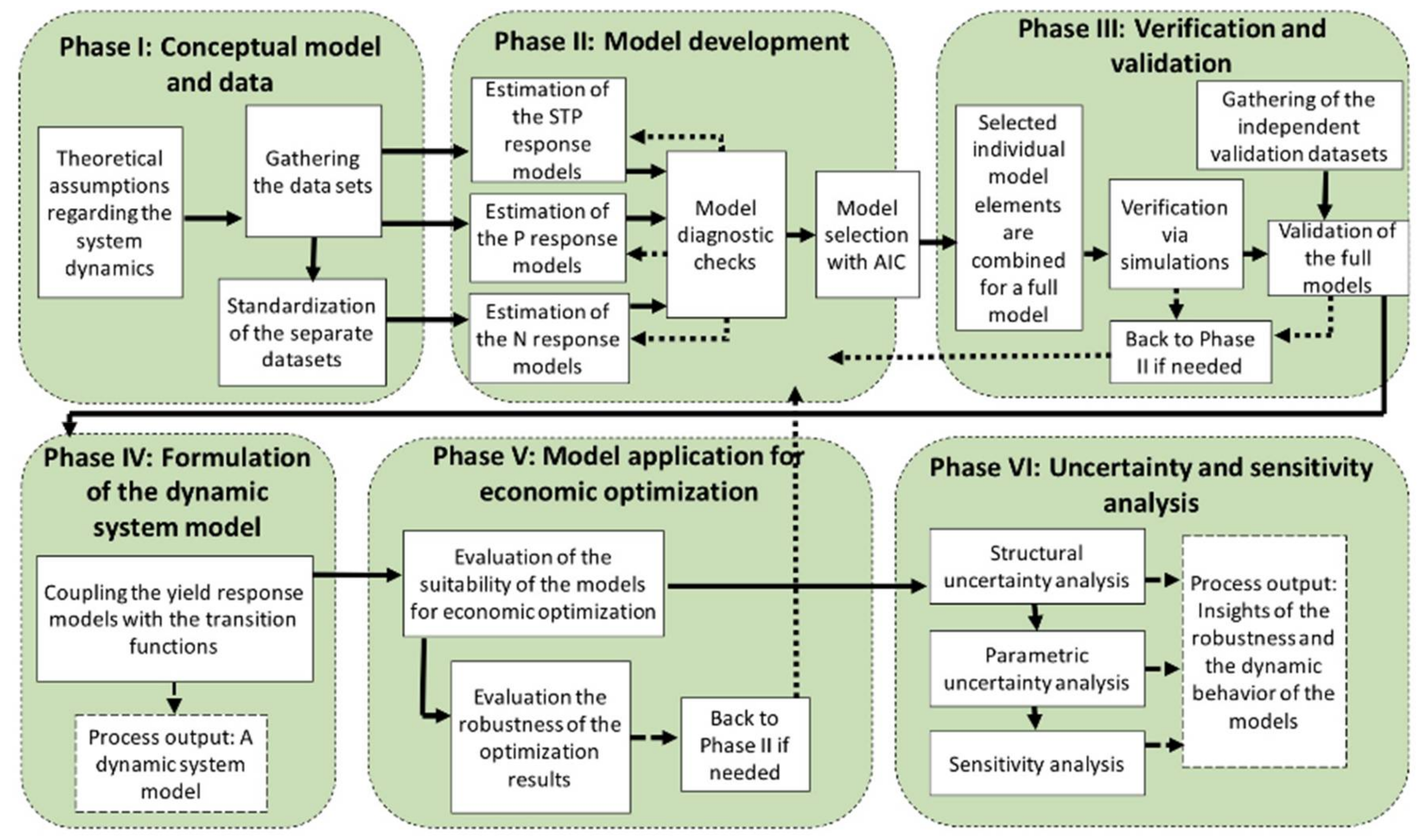
Figure 2.
The conceptual farm-level dynamic decision model (adapted from Hardaker et al. [49]), where t denotes a stage (one year), STP is the soil test P, which is the state of the system, P and N denote annual input decisions, R denotes the annual state return, r is the stage return function, y is the annual crop yield, p denotes the prices of inputs and output, and denotes a transition function that determines the evolution of the system from one stage to the next.

Figure 3.
Above the simulated yield N-P-response surfaces for the fair STP class for (a) coarse and (b) clay soils. Below the yield as a function of STP for various P and N rates for (c) coarse and (d) clay soils.
Figure 3.
Above the simulated yield N-P-response surfaces for the fair STP class for (a) coarse and (b) clay soils. Below the yield as a function of STP for various P and N rates for (c) coarse and (d) clay soils.
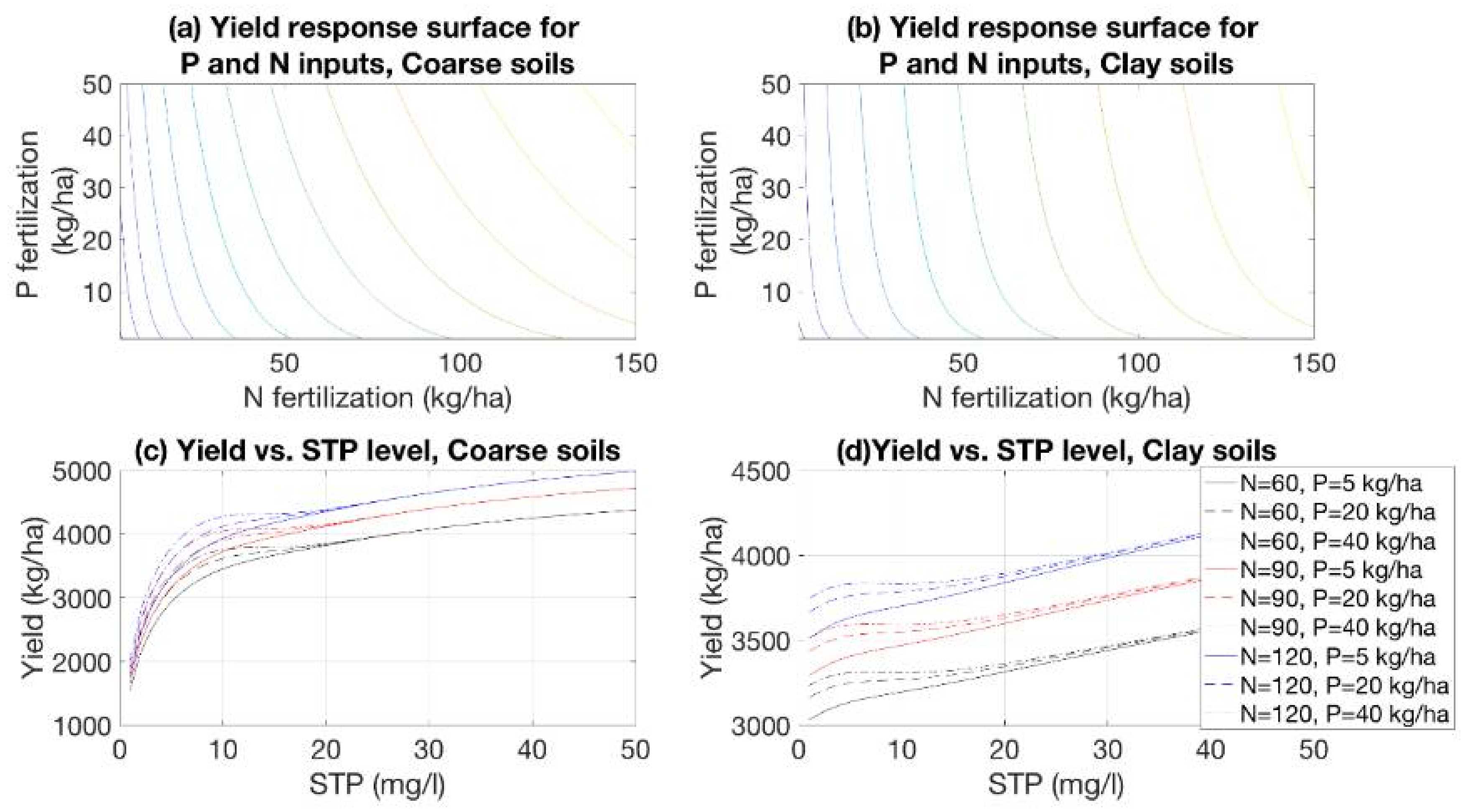
Figure 4.
Graphical model validation results for (a–c) coarse-textured soils and (d–f) clay soils.

Figure 5.
Steady-state yields for (a) coarse-textured soils and (c) clay soils determined by the different model candidates, and the associated economic losses resulting from incorrect model specification measured in differences in net present value (NPV) for (b) coarse and (d) clay soils. The dashed line indicates the level associated with the best model candidate.

Figure 6.
The effect the initial STP level on paths for STP development and for P and N fertilization for two fertilization management strategies.
Figure 6.
The effect the initial STP level on paths for STP development and for P and N fertilization for two fertilization management strategies.

Figure 7.
The relationship between the initial soil test P (STP) and net present value (NPV) for the cases where the fertilization paths were determined by economic optimization and by applying the present maximum permissible rates (100 kg N ha−1 a−1) and declining maximum permissible P rates for the increasing STP classes.
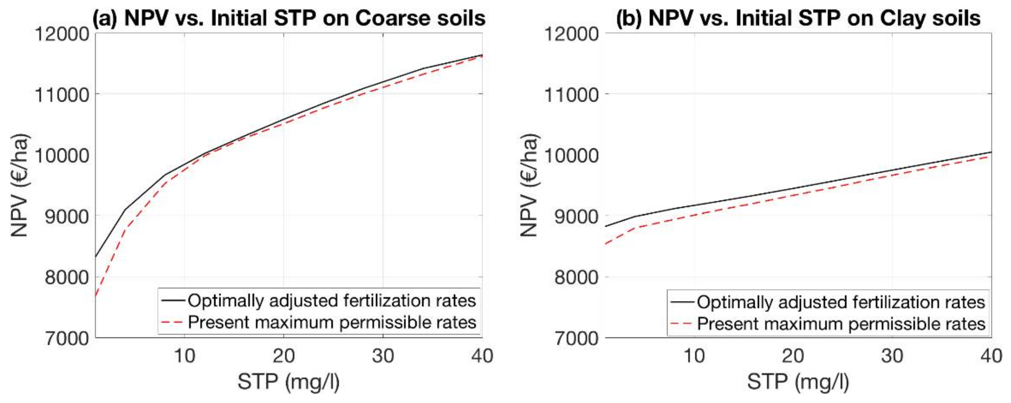
Table 1.
Parameters and the associated statistics for the models describing the yield response to soil test P (STP), P and N fertilization on coarse and clay soils as per Equations (15) and (16) †.
Table 1.
Parameters and the associated statistics for the models describing the yield response to soil test P (STP), P and N fertilization on coarse and clay soils as per Equations (15) and (16) †.
| Soil Texture | Parameter | Estimate | SD * | t-Value | P (>) |
|---|---|---|---|---|---|
| Coarse | 0.0133 | 4.535 × 10⁻⁴ | 29.37 | <2.2 × 10⁻¹⁶ | |
| 0.0797 | 0.0126 | 6.33 | 2.747 × 10⁻⁸ | ||
| 0.0095 | 0.0031 | 3.09 | 0.0029 | ||
| 0.727 | 0.0742 | 9.787 | 4.791 × 10⁻¹⁴ | ||
| 0.0269 | 0.00269 | 10.01 | 2.023 × 10⁻¹⁴ | ||
| 3.653 × 10⁻⁸ | 6.694 × 10⁻⁹ | 5.46 | 9.699 × 10⁻⁷ | ||
| Clay | 0.317 | 0.150 | 2.12 | 0.0493 | |
| 65.80 | 1.248 | 52.74 | <2.2 × 10⁻¹⁶ | ||
| 0.0372 | 0.0041 | 9.08 | 2.93 × 10⁻¹¹ | ||
| 0.010 | 0.0045 | 2.232 | 0.0313 | ||
| 0.0799 | 0.021 | 3.81 | 6 × 10⁻⁴ | ||
| 0.0377 | 0.0048 | 7.91 | <2.2 × 10⁻¹⁶ |
† The standard errors are heteroscedasticity-and-autocorrelation-consistent (HAC) for the coarse soils. In the case of first model element for the clay soils, the parameters were estimated via bootstrapping since the data sample was small. For the second model element, the standard errors were not HAC since the distribution of the residual errors was not significantly different from a normal one. Nonlinear mixed-effect (nlme) estimation was applied to the third model element.
Table 2.
Evaluation of the goodness-of-fit between the yield response models and the initial datasets †.
Table 2.
Evaluation of the goodness-of-fit between the yield response models and the initial datasets †.
| Soil Texture | Number of the Model Element ‡ | NSE | RMSE | MB | MAE | |
|---|---|---|---|---|---|---|
| Coarse | (1) | 0.62 | 0.36 | 939 (29%) | −65 (2.0%) | 811 (25.2%) |
| (2) | 0.8 | 0.63 | 0.07 (6.5%) | 0.01 (0.9%) | 0.05 (4.6%) | |
| (3) | 0.87 | 0.76 | 0.09 (9.2%) | 0.01 (1.0%) | 0.07 (7.2%) | |
| Clay | (1) | 0.46 | 0.21 | 630 (2.3%) | 32.28 (0.8%) | 458.1 (12%) |
| (2) | 0.76 | 0.54 | 0.04 (3.8%) | 0.005 (4.7%) | 0.03 (2.9%) | |
| (3) | 0.94 | 0.89 | 0.08 (8.5%) | 0.01 (0.6%) | 0.06 (6.4%) |
† Pearson’s product-moment correlation coefficient between measured and simulated values is indicated by r, NSE is Nash−Sutcliffe efficiency, RMSE is root mean squared error, MB is the mean bias, and MAE is the mean absolute error. The statistics are a percentage of the observed mean values, in brackets. ‡ Model Element (1) refers to Equation (2), Model Element (2) refers to Equation (3), and Model Element (3) refers to Equation (4).
Table 3.
Evaluation of the goodness-of-fit between the model simulations and the observations in the validation datasets †.
Table 3.
Evaluation of the goodness-of-fit between the model simulations and the observations in the validation datasets †.
| Soil Texture | r | NSE | RMSE | MAE | MB |
|---|---|---|---|---|---|
| Coarse | 0.81 | 0.66 | 452 (12%) | 338 (9.2%) | 21.1 (0.6%) |
| Clay | 0.76 | 0.54 | 706 (21%) | 564 (17%) | 132 (4%) |
† The mean-normalized statistics are shown in brackets. Pearson’s product-moment correlation coefficient between measured and simulated values is indicated by r, NSE is Nash−Sutcliffe efficiency, RMSE is root mean squared error, MAE is the mean absolute error, and MB is the mean bias.
Table 4.
Summary of the statistical tests for the model validation results.
| Soil Texture | Test | Test Statistic | p-Value |
|---|---|---|---|
| Coarse | Shapiro−Wilk normality test | 0.95 | 0.124 |
| t-test for coefficient in Equation (5) | −35.9 | 0.96 | |
| t-test for coefficient in Equation (5) | 1.004 | 3.66 × 10⁻⁶ | |
| Paired t-test | −0.124 | 0.902 | |
| Clay | Shapiro−Wilk normality test | 0.98 | 0.55 |
| t-test for coefficient in Equation (5) | −713 | 0.119 | |
| t-test for coefficient in Equation (5) | 1.17 | 7.155 × 10⁻¹³ | |
| Paired t-test | −0.87 | 0.39 |
Table 5.
Steady states obtained by applying economically optimal fertilization rates and the maximum permissible fertilizer rates of the voluntary agro-environmental scheme in Finland †.
Table 5.
Steady states obtained by applying economically optimal fertilization rates and the maximum permissible fertilizer rates of the voluntary agro-environmental scheme in Finland †.
| Soil Texture | Variable ‡ | Values Characterizing the Steady State | |
|---|---|---|---|
| Values Obtained by Dynamic Optimization | Values Obtained by Simulating the Model Using the Present Maximum Permissible Fertilization Rates § | ||
| Coarse | N rate (kg N ha−1 a−1) | 95.8 | 100 |
| P rate (kg P ha−1 a−1) | 21.7 | 16 | |
| STP (mg P l−1 a−1) | 9.88 | 7.85 | |
| Yield (kg ha−1 a−1) | 3958 | 3795 | |
| Profit (€ ha−1 a−1) | 345 | 333 | |
| NPV (€ ha−1) | 9614 | 9446 | |
| Clay | N rate (kg N ha−1 a−1) | 102.4 | 100 |
| P rate (kg P ha−1 a−1) | 6.75 | 16 | |
| STP (mg P l−1 a−1) | 3.86 | 6.81 | |
| Yield (kg ha−1 a−1) | 3509 | 3603 | |
| Profit (€ ha−1 a−1) | 314.3 | 309.6 | |
| NPV (€ ha−1) | 9006 | 8809 | |
† The exemplary fixed prices are 0.91€ kg−1, 1.99€ kg−1, and 0.12€ kg−1, for N, P, and barley, respectively. The discount rate is 3.5% and the initial STP levels are 7.5 mg L−1 and 4.5 mg L−1 for coarse and clay soils, respectively. ‡ STP indicates soil test P and NPV indicates net present value. § The present maximum permissible N rate is 100 kg ha−1 and that of P is 34 kg ha−1 for the poor STP class, 26 kg ha−1 for the rather poor STP class, 16 kg ha−1 for the fair STP class, 10 kg ha−1 for the satisfactory STP class, 5 kg ha−1 for the good STP class, and 0 kg ha−1 for the high and excessive STP classes [69].
Table 6.
Effect of the structural uncertainty on the robustness of the economic optimization results †.
Table 6.
Effect of the structural uncertainty on the robustness of the economic optimization results †.
| Soil Texture | Variable ‡ | Average Steady-State Value (95% CI) | Range (min, max) | SD/Average |
|---|---|---|---|---|
| Coarse | N rate (kg N ha−1 a−1) | 103 (73.7, 132) | (82.8, 125) | 0.139 |
| P rate (kg P ha−1 a−1) | 22.8 (19.6, 26) | (19.6, 25.7) | 0.07 | |
| STP (mg P l−1 a−1) | 10.1 (8.96, 11.2) | (9.08, 10.9) | 0.055 | |
| Yield (kg ha−1 a−1) | 4100 (3790, 4410) | (3852, 4421) | 0.037 | |
| Profit (€ ha−1 a−1) | 353 (342, 364) | (343, 366) | 0.016 | |
| NPV (€ ha−1) | 9846 (9503, 10190) | (9568, 10200) | 0.017 | |
| NPV (€ ha−1) | −31.8 (−86.9, 23.3) | (−92.3, 0) | −0.85 | |
| Clay | N rate (kg N ha−1 a−1) | 95.2 (84.9, 105) | (86.2, 103) | 0.053 |
| P rate (kg P ha−1 a−1) | 5.96 (1.01, 10.9) | (1.71, 9.36) | 0.41 | |
| STP (mg P l−1 a−1) | 3.79 (2.64, 4.93) | (2.81, 4.64) | 0.15 | |
| Yield (kg ha−1 a−1) | 3412 (3221, 3602) | (3241, 3546) | 0.027 | |
| Profit (€ ha−1 a−1) | 311 (303, 319) | (304, 317) | 0.013 | |
| NPV (€ha−1) | 8914 (8709, 9119) | (8730, 9068) | 0.011 | |
| NPV (€ ha−1) | −44.25 (−168, 79.54) | (−171.3, 0) | −1.37 |
† The number of the model candidates was 30 for coarse soils and 32 for clay soils. ‡ STP indicates soil test P, NPV indicates net present value, and NPV indicates the difference in NPV between the best model candidate and any other model candidate.
Table 7.
Summary of the Monte Carlo analysis results used for examining the effect of the parametric uncertainty on model output (the barley yield), associated with individual model elements and the entire model for coarse and clay soils †.
Table 7.
Summary of the Monte Carlo analysis results used for examining the effect of the parametric uncertainty on model output (the barley yield), associated with individual model elements and the entire model for coarse and clay soils †.
| Soil Texture | Model Element Subject to Parametric Uncertainty | Average Yield (95% CI) | SD (95% CI) | 95% CI (for Mean Values) | SD/Average |
|---|---|---|---|---|---|
| kg ha−1 a−1 | |||||
| Coarse | First model element | 3947 (+/−5) | 270 (+4, −3) | (3397, 4497) | 0.068 |
| Second model element | 3938 (+/−2) | 101 (+2, −1) | (3732, 4144) | 0.026 | |
| Third model element | 3936 (+/−6) | 303 (+/−4) | (3319, 4553) | 0.077 | |
| Entire model | 3955 (+7, −9) | 421 (+/−6) | (3099, 4811) | 0.106 | |
| Clay | First model element | 3518 (+5, −6) | 281 (+/−4) | (2967, 4069) | 0.08 |
| Second model element | 3509 (+/−1) | 41(+/−0.6) | (3429, 3589) | 0.012 | |
| Third model element | 3567 (+/−12) | 636 (+/−11) | (2320, 4814) | 0.178 | |
| Entire model | 3578 (+/−14) | 702 (+/−12) | (2201, 4954) | 0.196 | |
† During Monte Carlo analysis, the values for N, P, and STP were fixed to their economically optimal steady state levels as shown in Table 5. The asymptotic 95% CI for the average yield and its standard deviations illustrate the uncertainty of the statistic. ‡ The first model element refers to Equation (2), the second model element refers to Equation (3), and the third model element refers to Equation (4).
© 2018 by the authors. Licensee MDPI, Basel, Switzerland. This article is an open access article distributed under the terms and conditions of the Creative Commons Attribution (CC BY) license (http://creativecommons.org/licenses/by/4.0/).
Share and Cite
MDPI and ACS Style
Sihvonen, M.; Hyytiäinen, K.; Valkama, E.; Turtola, E. Phosphorus and Nitrogen Yield Response Models for Dynamic Bio-Economic Optimization: An Empirical Approach. Agronomy 2018, 8, 41. https://doi.org/10.3390/agronomy8040041
AMA Style
Sihvonen M, Hyytiäinen K, Valkama E, Turtola E. Phosphorus and Nitrogen Yield Response Models for Dynamic Bio-Economic Optimization: An Empirical Approach. Agronomy. 2018; 8(4):41. https://doi.org/10.3390/agronomy8040041
Chicago/Turabian StyleSihvonen, Matti, Kari Hyytiäinen, Elena Valkama, and Eila Turtola. 2018. "Phosphorus and Nitrogen Yield Response Models for Dynamic Bio-Economic Optimization: An Empirical Approach" Agronomy 8, no. 4: 41. https://doi.org/10.3390/agronomy8040041
Note that from the first issue of 2016, this journal uses article numbers instead of page numbers. See further details here.