Assessing Olive Evapotranspiration Partitioning from Soil Water Balance and Radiometric Soil and Canopy Temperatures

ICAAM-Instituto de Ciências Agrárias e Ambientais Mediterrânicas, Universidade de Évora, Núcleo da Mitra, Ap. 94, 7002-554 Évora, Portugal
Agronomy 2018, 8(4), 43; https://doi.org/10.3390/agronomy8040043
Submission received: 8 March 2018
/
Revised: 3 April 2018
/
Accepted: 5 April 2018
/
Published: 6 April 2018
(This article belongs to the Special Issue Sensing and Automated Systems for Improved Crop Management)
Abstract
:Evapotranspiration (ETc) partitioning and obtaining of FAO56 dual crop coefficient (Kc) for olive was carried out with the SIMDualKc software application for root zone and topsoil soil water balance based on the dual crop coefficients. A simplified two source-energy balance model (STSEB), based on daily remotely sensed soil and canopy thermal infrared data and retrieval of surface fluxes, also provided information on partitioning ETc for the olive orchard. Both models were calibrated and validated with ground-based, sap flow-derived transpiration rates, and their performance was compared in partitioning ETc for incomplete cover, intensive olive grown in orchards (≤300 trees ha−1). The SIMDualKc proved adequate in partitioning ETc. The STSEB model underestimated ETc mostly by inadequately simulating soil evaporation and its contribution to the total latent heat flux. Such results suggest difficulties in using information from the STSEB algorithm for assessing ETc and dual Kc crop coefficients of intensive olive orchards with incomplete ground cover.
1. Introduction
A reliable assessment of olive water requirements at different stages in the olive’s development is particularly relevant for the correct estimation of daily water needs and the improvement of irrigation management. For deficit irrigation (DI) scheduling routines applied to olives to reduce production costs, improve fruit quality, and save water [1], such knowledge is particularly relevant to avoid severe water stress on sensitive phases of the growing period [2,3,4,5,6], as the responses to DI regimes are often variable, depending on the timing and severity of water deficits [2,7]. So, the precise monitoring of actual olive water use throughout the irrigation cycle is of utmost importance. The usual approach for the estimation of crop water requirements is the crop coefficient Kc-ETo approach adopted by FAO56 [8]. Single and dual crop coefficient Kc values are defined and tabulated by FAO56 [8,9] for a wide range of agricultural crops, with Kc expressing differences between reference and target crop in terms of ground cover, canopy properties, and aerodynamic resistance. In the single approach, both crop transpiration (T) and soil evaporation (Es) components of crop ETc are timely averaged into a single coefficient (Kc), whereas in the dual approach, the Kc coefficient is the separate sum of a daily basal crop coefficient (Kcb), representing the plant transpiration, and a daily soil evaporation coefficient (Ke). Usage of the dual Kc approach is particularly appealing in two counts; it allows for the partitioning of ETc and the estimation of potential, non-stressed transpiration, T, which is more suitable for irrigation management purposes, as it closely relates to crop yield [7,10,11,12], and the estimation of soil evaporation, whose accuracy is improved with the procedure [12,13]. For crops with incomplete ground cover, such as olive, Allen and Pereira [9] further refined the concept of dual Kc, and tabulated sets of Kc and Kcb values for orchards and vines by taking into account their planting density, canopy size and height, and active understory growing vegetation. For deficit irrigation strategies that impose some degree of stress to crops, such as in olive irrigation, they adjusted the traditional FAO56 approach to estimate ETc with the dual crop coefficient method by replacing the potential ETc with an actual ETc (ETc act), the result of a Kc act coefficient derived from a stress coefficient (Ks), and a soil evaporation coefficient Ke, i.e., Kc act = KsKcb + Ke. The multiplier Ks is equal to 1.0 for no soil water stress and less than 1.0 with water stress conditions. To estimate Ks and Ke, water balance calculations for the root zone and the topsoil are required on a daily basis, which often entails an appropriate computational model framework [9,14]. The SIMDualKc model [15,16,17] provides such computational structure by incorporating the most recent refinements in the concept of dual crop coefficients and by performing the required soil water balance, to provide information on the stress coefficient Ks, on potential and actual Kcb, on Ke, and finally on potential and actual Kc. The results of using the model compared well with field observations for annual, vine, and woody crops [11,13,17,18,19,20,21,22,23]. The SIMDualKc approach on olives has focused on comparing daily transpiration simulated data with those obtained with sap flow measurements [17,18,19,24], and has been applied exclusively to super high-density olive orchards (≥1500 trees ha−1). The merits of this application to intensive orchards (≤300 trees ha−1) with larger incomplete ground cover such as the one in this study remain uncertain.
Other than using the SIMDualKc soil water balance for partitioning ETc, the partition is traditionally performed by classic processes grounded on the two-source (soil + vegetation) layer surface energy balance models [25,26,27,28,29,30,31,32]. A simpler version of the two-source configuration (STSEB) has been more recently proposed by [33] and successfully used in assessing the ETc act and the corresponding Kc act of cover crops [34,35]. Based on remotely sensed thermal infrared data and retrieval of surface fluxes, the framework computes T and Es, and hence ETc, as residuals to the components soil and vegetation energy-balance budgets directly from measured soil (Ts) and canopy (Tc) radiometric temperatures. The success of the developed STSEB relationships in partitioning and establishing accurate ETc values from the soil and canopy contributions to the total sensible heat flux has been established mainly for herbaceous crops, such as corn [33], sorghum [35], sunflower, and canola [34]. No studies were found evaluating the strength of the STSEB relationships in predicting ETc for fruit trees, in particular, olives.
In consideration of the above-mentioned methods and techniques and the need to obtain accurate information on actual ETc partitioning and related dual Kc crop coefficients for better irrigation management of intensive olive orchards grown in southern Portugal, a region of scarce water resources where water plays a decisive role in agricultural development and imposes the optimization of olive-growing irrigation water use, the main objectives of this study were: (1) to test and validate the simplified version of the two-source configuration (STSEB) for olives from thermal infrared radiometry, ancillary meteorological data, and sap flow field measurements; (2) to test and validate the SIMDualKc model with data from sap-flow field measurements; (3) to assess and compare actual olive T, Es, and ETc with information derived from the STSEB and SIMDualKc energy- and water-balance models.
2. Material and Methods
2.1. Study Site and Measurements
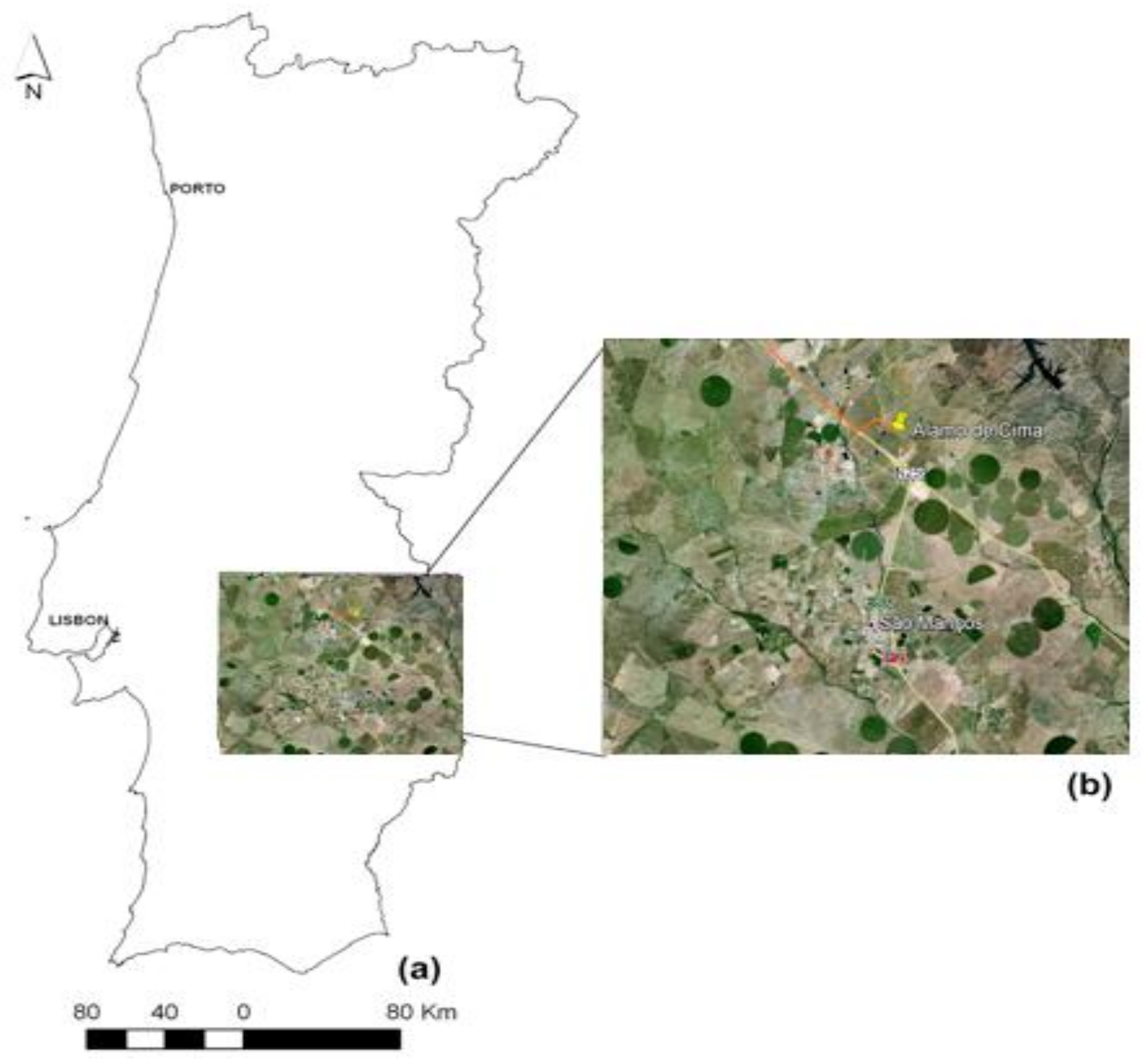
The experiments were carried out in an intensive commercial olive orchard at the Herdade Álamo de Cima, near Évora (38°29′49.44′’ N, 7°45′8.83′’ W; alt. 75 m) in southern Alentejo, Portugal. The orchard was established with 10-year old trees in grids of 8.0 × 4.2 m (300 trees ha−1) in the E-W direction. Climate in the region is typically Mediterranean, with long-term average annual rainfall of around 650 mm, mostly distributed from September/October to May, with the remaining summer months dry and hot. Half-hour average of the meteorological parameters wind speed, air temperature, solar radiation, precipitation, and relative humidity were evaluated from data recorded in an automatic weather station adjacent to the orchard, equipped with a solar panel and a standard set of sensors recording maximum and minimum air temperature, relative humidity, wind speed and wind direction, barometric pressure, solar radiation, and precipitation. Daily values of ETo were calculated using the FAO-Penman–Monteith equation and the procedures prescribed in [8]. The average values for the 2-year experimental period (2013 and 2014) of potential evapotranspiration (ETo) and precipitation (P) were 1161.0 mm and 791.0 mm, respectively. Half-hour average of thirty seconds net radiation above the canopy of trees was obtained throughout the irrigation cycle using one NrLite net radiometer (Kipp & Konen, Delft, The Netherlands) connected to a data logger (Delta-T, DL2e, Delta-T Devices, Cambridge, UK). Collected ground data included fraction of ground shaded by canopy (fc) and tree height, whose measurements were used to calibrate and validate both models. The fc was approximately 0.28, and tree height was around 3.5 m. The procedure to obtain fc was based upon measurements in 35 randomly selected trees of the projection of their crown diameters. Soils are sandy loam Regosoil Haplic of weakly developed and unconsolidated materials [36]. The average apparent bulk soil density was 1.52 Mg m−3, and average volumetric soil water content at 0.03 MPa was 0.28 m3 m−3, whereas it was 0.16 m3 m−3 at 1.5 MPa. The average total available soil water in the root zone (TAW) was 194 mm for a soil depth of 1.2 m. The olive orchard was typically irrigated almost every day, during spring and summer, with a drip system having emitters with 1.0 m spacing along the row and discharging 2.3 L h−1 (0.27 mm h−1). In general, irrigation season started in March/April and ended in September/October. The average daily irrigation amounts were close to 4.2 mm d−1 during the two irrigation seasons. Irrigation dates and depths were provided by the farm manager and were locally measured with a tipping-bucket rain gauge (ARG100, Environmental Measurements Ltd., Sunderland, UK) connected to recording data loggers. Figure 1 shows the study area location in southern Portugal (a) and the intensive commercial orchard where experiments were carried out (b).
2.2. Field Data
Data obtained from ground-based measurements were used to validate information obtained with the SIMDualKc and STSEB simulation models. Olive daily sap flow-based transpiration rates (Tsf) on a ground area basis (mm d−1) were assessed for the 2-year experimental seasons using sap flow measurements by the Compensation Heat Pulse method [37,38]. A set of six heat-pulse probes (Tranzflo, Palmerston, New Zealand) was distributed by seriated trees, according to trunk diameter class frequency, established in a larger sample of the plot [17] and continuously monitored from the period 113 to 304 DOY (day of year) in 2013, and 126 to 278 DOY in 2014. Thirty-minute data were stored in a datalogger (Model CR1000, Campbell Scientific, Inc., Logan, UT, USA). Heat-pulse (ideal) velocity was corrected for probe-induced wounding effects in the trunk near the probes using coefficients after [39]. To calibrate and validate the SIMDualKc and STSEB models, and support the derivation of olive crop coefficients, which is analyzed in Section 3, daily sap flow-based transpiration data were used, thus comparing transpiration rates simulated by SIMDualKc (TSDual) and STSEB (TSTSEB) with derived Tsf (n = 146 in 2013 for calibration and n = 146 in 2014 for validation). Radiometric soil (Ts) and canopy (Tc) surface temperatures were measured according to procedures in [34]. Apogee S-111 thermal infrared radiometers (IRT) were used. One was placed at a height of 2.0 m above the canopy level, looking at the surface with nadir view, and a second radiometer was placed between rows, directly pointing to the soil at 0.40 m height and 1.2 m distance from the tree row, respectively. A third IRT was placed at 2.0 m above canopy height at an angle of 53° to measure sky brightness temperature. Data were used for atmospheric correction of the surface temperature (Apogee Instruments, Logan, UT, USA, 2016), as the STSEB model requires calibrated thermal-infrared observations adjusted for atmospheric effects and corrected for surface emissivity in the thermal infrared band to produce accurate results. All thirty-minute data were stored in dataloggers (Model CR1000, Campbell Scientific, Inc., Logan, UT, USA). IRT measurements were limited to year 2014 and were collected for the period 163 to 304 DOY. An independent energy balance between the atmosphere and each component of the surface was established, leading to daily values of soil evaporation (EsSTSEB) and olive transpiration (TSTSEB), as discussed below.
Incident daily photosynthetically active radiation (PAR) and the fraction of PAR intercepted by the canopy were obtained from logged (CR10X, Campbell Scientific, Inc., Logan, UT, USA) measurements (umol m−2 s−1) of a set of six Quantum sensors (QPAR-02, 400–700 nm, Tranzflo, Palmerston, NZ, USA) placed in a fixed transect of three sensors on each side (East and West) of the tree line (N-S) at 0.2, 1.0, and 1.88 m, respectively, with one placed on top of the canopy (5.0 m). On clear sky days, leaf area index (LAI) measurements were taken periodically with a ceptometer (Accupar-LP80, Decagon Devices Inc., Pullman, WA, USA) that takes into account the canopy’s leaf distribution to make the calculation of LAI an instant measurement from the radiation measurements. We followed the measurement strategy proposed in [40] for olive orchards. Half-hour average of thirty seconds net radiation above the canopy of trees was obtained throughout the irrigation cycle using one NrLite net radiometer (Kipp & Konen, Delft, The Netherlands) connected to a data logger (Delta-T, DL2e, Delta-T Devices, Cambridge, UK). Mean weather variables for both study seasons are shown in Table 1. The olive trees are of cultivar Cobrançosa.
2.3. The STSEB Simplified Energy Balance Model
The simplified version (STSEB) of the two-source modeling configuration for computing surface fluxes using soil and canopy temperature observations introduced by [34] was used in this study. According to the approach described in [34], the latent heat flux, λETc, represents the energy required for ETcSTSEB and is computed as the residual of the following surface energy balance simplified form,
in which Rn is the net radiation flux (W m−2), H is the sensible heat flux (W m−2), and G is the soil heat flux (W m−2). Soil and canopy sensible fluxes, Hs (W m−2) and Hc (W m−2), weighed by their partial cover areas, add to total sensible flux, H, as:
A complete and independent energy balance between the atmosphere and each component of the surface is then established by the following relationships:
in which λEsSTSEB and λTSTSEB are the energy required for soil evaporation, EsSTSEB, and canopy transpiration, TSTSEB, respectively. Calculated λEsSTSEB, and λTSTSEB, and λETcSTSEB are converted to soil evaporation (EsSTSEB), plant transpiration (TSTSEB), and evapotranspiration (ETcSTSEB), respectively, by means of the latent heat of vaporization, λ, (MJ kg−1). The energy connected to soil warming, G, is estimated as a fraction (CG) of the soil contribution to the net radiation as follows, in which CG can vary in a range of 0.2–0.5 depending on the soil type and moisture.
Net radiation is computed from a balance between the incoming and outgoing short-wave and long-wave radiances, in which Rnc and Rns are the contributions of the canopy and soil, respectively, to the total net radiation flux.
in which α and ε are the surface parameters albedo and emissivity, respectively, σ is the Stefan-Boltzman constant, S is the solar radiation (W m−2), and Lsky (W m−2) is the incident long-wave radiation, Tc and Ts, and the canopy and soil surface temperatures (K). The soil and canopy contributions to the total sensible heat flux, Hs and Hc, respectively, are expressed as:
in which ρCp is the volumetric heat capacity of air (J K−1 m−3), Ta is the air temperature at a reference height (K), is the aerodynamic resistance to heat transfer between the canopy and the reference height at which the atmospheric data are measured (s m−1), is the aerodynamic resistance to heat transfer between the point zOM + d (zOM: canopy roughness length for momentum, and d: displacement height) and the reference height (s m−1), and is the aerodynamic resistance to heat flow in the boundary layer immediately above the soil surface (s m−1). We used expressions to estimate the resistances reported in [33]. Using daily radiometric temperatures data collected in 2014, together with the meteorological variables wind speed, solar and long-wave radiation, and biophysical information on canopy height and fractional vegetation cover as inputs in the above equations, we obtained results of the different terms of the energy balance equation for every 30 min. Modeled daily values of transpiration (TSTSEB) were then tested by comparison with field observed sap flow daily transpiration rates (Tsf). To further test the performance of the STSEB model, these findings, as well as soil evaporation (EsSTSEB) and evapotranspiration (ETcSTSEB) results, were compared with related 2014 SIMDualKc results, and their recognized robustness in modeling soil evaporation and crop evapotranspiration was considered [20,21].
2.4. The SIMDualKc Water Balance Model
The SIMDualKc is a soil water balance model that applies the dual crop coefficient approach to simulate ETc, the basal (Kcb) and soil evaporation (Ke) coefficients that relate to crop transpiration (Tc), and soil evaporation (Es), respectively, as:
in which ETcSDual is crop evapotranspiration for no stress conditions. When water stress occurs, ETcSDual is adjusted as a function of the available soil water in the root zone by considering a stress coefficient (KsSDual), thus providing ETcSDual act (mm d−1), which is the actual evapotranspiration.
in which KsSDual, the water stress coefficient, is an indicator of the relative intensity of the stress effect on a specific growth process and growth stage. The coefficient KsSDual is in essence a modifier of the parameter KcbSDual and ranges in value from one (no stress) to zero (full stress). The coefficient is often used to adjust ETcSDual to reflect the soil water conditions [9,16]; it is computed by SIMDualKc through a daily soil water balance algorithm for the entire root zone, and as a function of root zone water depletion. Concerning adjustments of FAO crop coefficients [12], the model takes into account plant density and height [9], through a density coefficient Kd, to better adjust the final computations of KcSDual or KcbSDual.
in which KcSDualfull is the estimated basal KcbSDual during the peak plant growth for conditions of full ground cover, and KcSDualmin is the minimum KcSDual for bare soil [16,17]. Kd is estimated from the effective fraction of ground cover as:
in which fc eff is the effective fraction of ground covered or shaded by vegetation near solar noon, ML is a multiplier on fc eff describing the effect of canopy density on shading and on maximum relative ETc per fraction of ground shaded, and h (m) is the mean height of the vegetation.
As previously mentioned, measured sap flow data (Tsf) from 2013 was used to calibrate the SIMDualKc model, and validation was performed with 2014 collected Tsf data. Table 2 shows the standard and calibrated parameters used in SIMDualKc model. In the calibration and validation processes, we used the methodologies and procedure described in [15,16,17].
2.5. Statistical Analysis
Agreement between observed and measured values, as well as the goodness of fit, was assessed in terms of the Willmot [41] index of agreement (WIA, dimensionless), the root mean squared error (RMSE), mean absolute error (MAE), average absolute error (AAE), and mean bias error (MBE). The software StatPlus, AnalystSoft Inc. version 6 was used.
3. Results and Discussion
3.1. Validation of the SIMDualKc Model
As stated previously, the SIMDualKc model was calibrated with data of 2013 and validated with data of the year 2014. The values of all initial and calibrated parameters are presented in Table 2. Model results are analyzed in detail in Section 3.3.
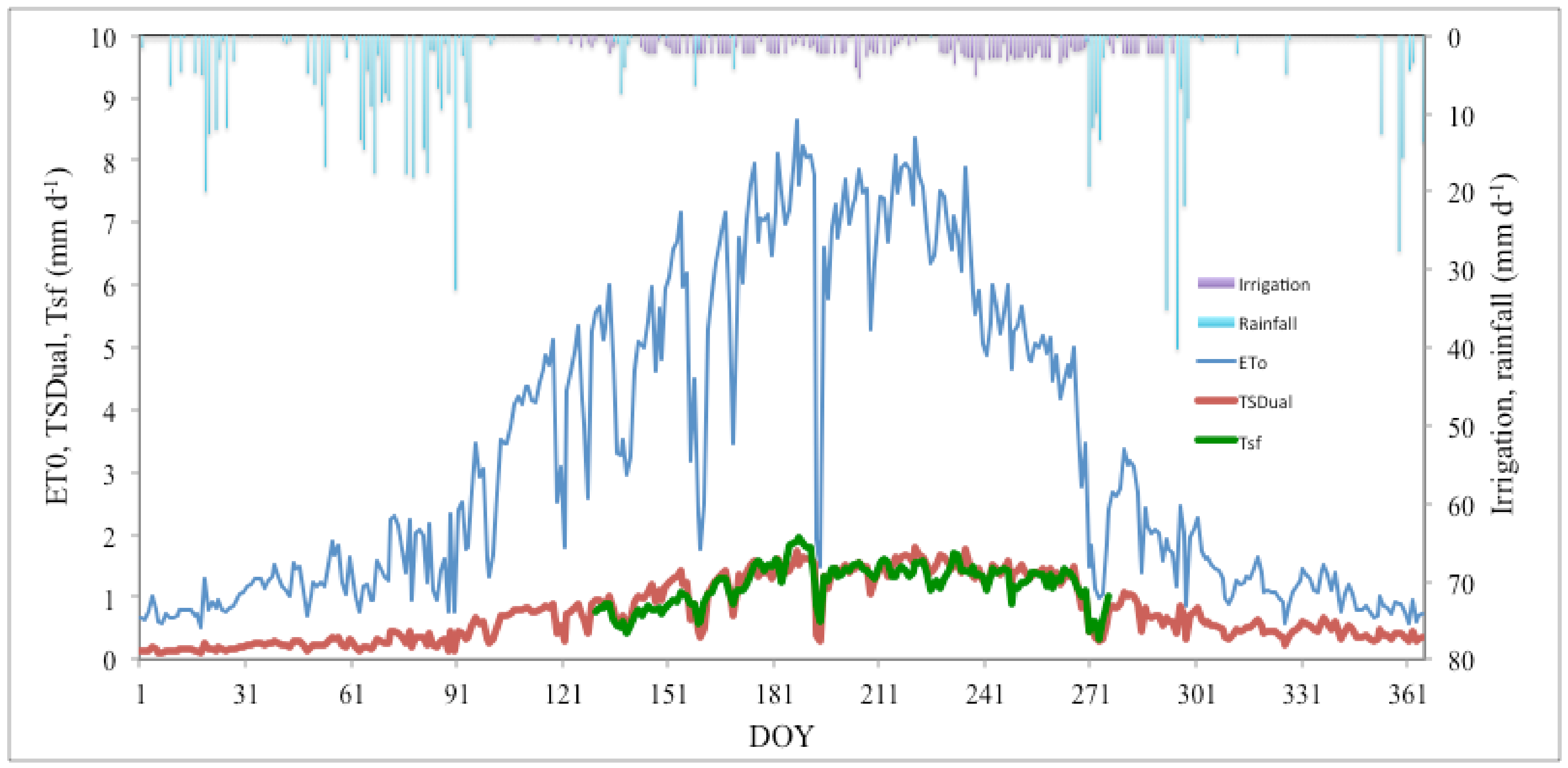
The comparison of transpiration data simulated by SIMDualKc (TSDUal) with observed data (Tsf), for the two years is shown in Figure 2, which includes ETo, rainfall, and irrigation data.
The data plots visually indicate that the model produces transpiration estimates close to observed data for the calibration year 2013, with no conspicuous patterns of deviations for the validation year 2014. Related goodness of fit and error indicators presented in Table 3 allow one to assume that SIMDualKc model performed well in capturing the characteristics of our intensive olive orchard of incomplete cover (≤300 trees ha−1), as it did for a super-intensive orchard (≥1500 trees ha−1) in the region, reported in [17,18]. 2014 observed (Tsf) and estimated transpiration data (TSDual) were compared (Figure 2) to validate the model.
Data show good correlation, with a higher determination coefficient (R2 = 0.81) and a regression coefficient b = 0.97, which is smaller than that for the calibration year (Table 3). Results indicate a slight underestimation but a strong explanation of data variance with overall goodness of fit data showing a good performance of the model during validation, with good agreement between TSDual and Tsf. Table 4 shows the mean modeled and observed transpiration values for the calibration and validation years (DOY 130 to 276, the period with available sap flow data).
Mean values were very similar in 2013 (1.25 and 1.21 mm d−1, respectively) and in 2014 (1.31 and 1.35 mm d−1). Minimum and maximum transpiration values in Table 4 were also quite close for both the calibration and validation years.
3.2. Validation TSTSEB with Field Sap Flow Transpiration Rates
Almost 960 half-hour canopy and soil surface temperature observations were obtained from DOY 166 to 273 and were used to run and evaluate the STSEB model output. For estimation of the contribution of canopy and soil, respectively, to the total net radiation flux, Equations (8) and (9) were applied using values of αs = 0.12, αc = 0.20, εs = 0.96, and εcs = 0.985, which were characteristics of the olive canopy [28,42,43]. The soil and canopy contributions to the total sensible heat flux, Hs and Hc, respectively, were evaluated with Equations (10) and (11). Related expressions, parameters, and constants to estimate the aerodynamic resistances were obtained from literature (Appendix A in [26,29,33,44] and ancillary meteorological and biophysical measurements of key variables to the STSEB model (vd. Section 2.1, and Section 2.2). The energy required for canopy transpiration and soil evaporation was evaluated with Equations (4) and (5), and the total energy balance was estimated with Equation (3). A constant value of CG = 0.35 was used in Equation (6), corresponding to the midpoint between its likely units [33,45]. Modeled daily values of transpiration (TSTSEB) were then tested by comparison with field observed sap flow daily transpiration rates (Tsf). The comparison is shown in Figure 3, with related goodness of fit indicators presented in Table 5.
Overall, simulated (TSTSEB) overestimate transpiration rates for values in-between 1.75 and 2.0 mm d−1 and underestimate them for lower values, indicated in the b = 0.99 coefficient of regression. Mean observed (Tsf) and simulated (TSTSEB) transpirations of 1.77 and 1.81 mm d−1, respectively, show the STSEB overestimation, also indicated in the percent value of the bias indicator PBIAS (−1.9%), with the negative sign referring to the occurrence of overestimation bias [14]. Generally, the statistical indicators show an acceptable performance of the model in simulating olive transpiration from July to mid-September, the region-relevant period for olive irrigation. To further test the performance of the STSEB model, soil evaporation (EsSTSEB) and evapotranspiration (ETcSTSEB) results are compared below with related 2014 results obtained with the validated SIMDualKc model. Additionally, simulated T, Es, and ETc with the two models are compared.
3.3. Assessing ETc with the SIMDualKc and STSEB Models
Series of ETc act (ETcSDual act) with the same length as simulated TSDual were obtained with SIMDualKc for 2014, with Figure 4 showing the time evolution of EsSDual, TSDual, and ETc act (ETcSDual act).
A mean EsSDual value of 0.56 mm d−1 is predicted for a maximum of 2.4 mm d−1 in DOY 177, a minimum of 0.02 mm d−1 in DOY 156, and a total of 202.2 mm for the year. Mean ETcSDual act of 1.4 mm d−1 (0.82 mm d−1 for TcSDual) is predicted for a maximum of 3.8 mm d−1 (1.89 mm d−1 for TSDual), a minimum of 0.31 mm d−1 (0.14 mm d−1 for TSDual), and a total of 500.8 mm for the year (298.6 mm for TSDual). The SIMDualKc approach to dual Kc for olives with incomplete ground cover takes into account the fraction of soil surface wetted by irrigation and exposed to radiation [46,12,19], hence reflected in the values of EsSDual [17,18].
Similarly, series of ETcSTSEB were obtained with STSEB model for 2014; the time evolution of EsSTSEB, TSTSEB, and ETcSTSEB for the period in-between June 15th and September 30th is presented in Figure 5.
A mean EsSTSEB value of 1.12 mm d−1 is predicted for a maximum of 1.36 mm d−1 in DOY 192, a minimum of 0.81 mm d−1 in DOY 265, and a total of 121.4 mm for the period. Mean ETcSTSEB of 1.33 mm d−1 (1.80 mm d−1 for TcSTSEB) is predicted for a maximum of 1.61 mm d−1 (2.21 mm d−1 for TSTSEB), a minimum of 0.95 mm d−1 (1.27 mm d−1 for TSTSEB), and a total of 143.4 mm for the period (194.8 mm for TSTSEB).
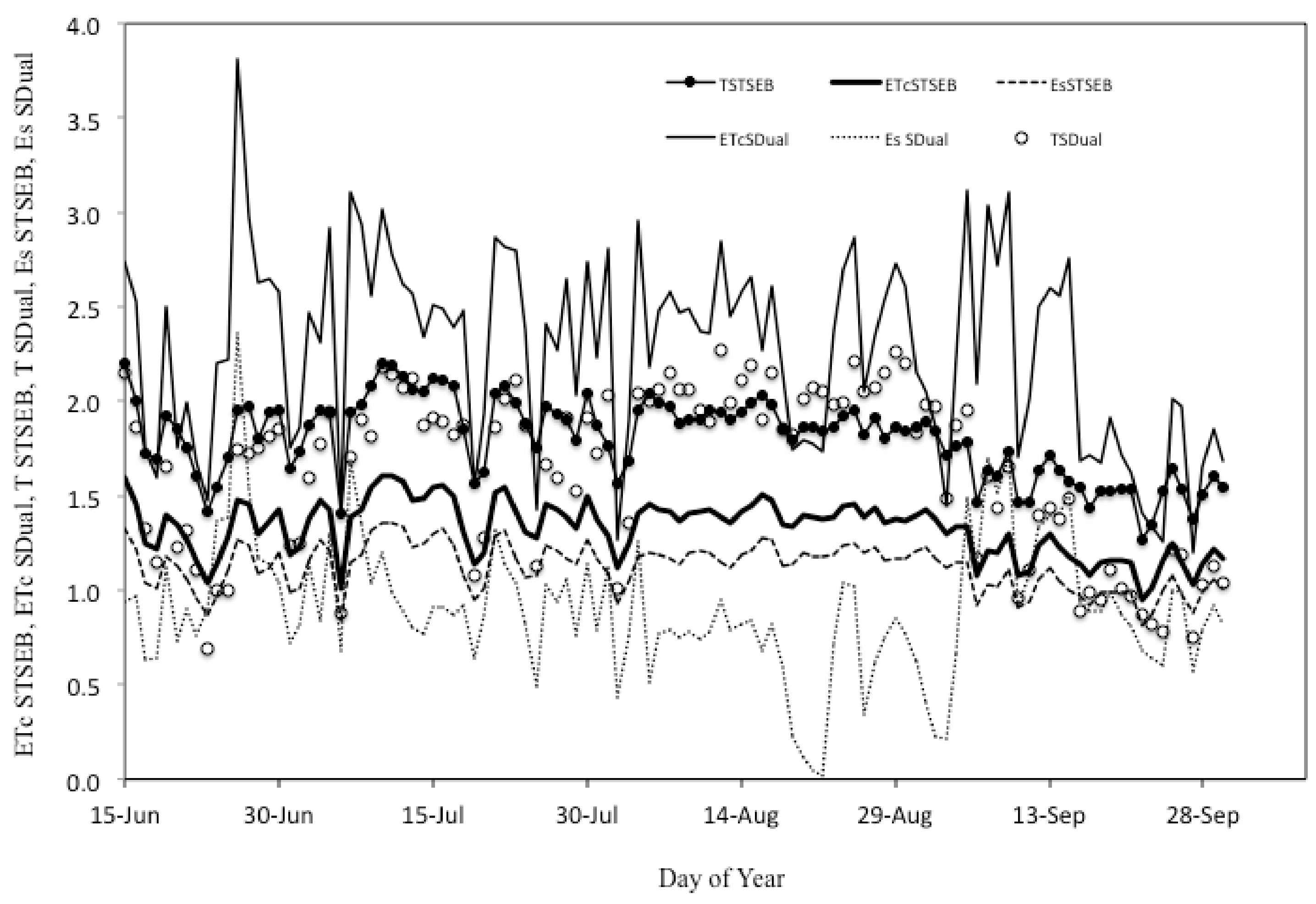
To further test the STSEB model, the ETcSTSEB simulated values with Equation (3) were compared to ETcSDual values. Figure 6 presents such values, as well as the TSDual, EsSDual, EsSTSEB, and TSTSEB plots.
The deviation of EsSTSEB from the values obtained with the SIMDualKc model is apparent. The mean EsSDual value of 0.89 mm d−1 (for a maximum of 2.36 mm d−1 and a minimum of 0.02 mm d−1) contrasts with the 1.12 mm d−1 value simulated with STSEB model (for a maximum of 1.36 and a minimum of 0.81 mm d−1), showing that simulated STSEB soil evaporation values stayed relatively high throughout the period, with a 0.55 mm d−1 difference between the maximum and minimum values, for a corresponding 2.24 mm d−1 difference with the SIMDualKc simulation. Moreover, ETcSTSEB values also considerably depart from simulated ETcSDual values. They stay always below TSTSEB values and very close to EsSTSEB values, which is an incongruity. The ratio of mean ETcSTSEB/ETcSDual = 0.56 and corresponding maximum and minimum ratios of 0.42 and 0.79, respectively, emphasize the inconsistency. Table 6 summarizes the results of actual ETc, T, and Es simulated with both models, in which the overestimation of TSTSEB for the entire period (TcSTEB of 194.8 mm vs. TcSDaul of 147.2 mm) and the high discrepancy between the total ETc (ETcSTEB of 143.4 mm vs. ETcSDaul of 245.1 mm) and Es values (ETsSTEB of 121.4 mm vs. ETsSDaul of 98 mm), are apparent.
In the latter above two cases, the source and main reason for the described inconsistencies appear to result from the built-in expectation in the STSEB model that the canopy geometry and evolution of fractional vegetation cover (fc) would rapidly progress as a function of the leaf area index (LAI) to a value close to 1, as it does for row crops [34,35]. Consequently, the estimated values of the fraction 1-fc, and EsSTSEB in Equation (3), would evolve to approach zero at the stage of complete ground cover by canopy, with TSTSEB weighted by its respective partial shaded area approaching 1.0, thus becoming the major contributor to ETc. In the case of our intensive olive orchard, with nearly constant fc (0.28 in our study) throughout the growing period, such assumption does not apply, leading to a clear underestimation of ETcSTSEB values (Figure 6, Table 6). Moreover, with practically constant values of EsSTEB estimated for the summer dry months (low or no rainfall, and efficient drip irrigation), the available energy for soil evaporation accounted for by Equation (5) does not in fact translate into a real soil evaporation, resulting in misleadingly high modeled soil evaporation results. As seen, the nearly constant ETsSTSEB values (mean of 1.12 mm d−1) are higher than the ones simulated with the SIMDualKc model (mean of 0.89 mm d−1), with the latter showing through the model soil surface water balance the existence of peaks and valleys from the occasional rainfall and the recurrent dry summer spells (Figure 4). Contrarily, the STSEB model, which tends to simulate nearly constant EsSTSEB values, shows EsSTSEB no reaction to the cycle of wet and dry spring and summer events. Moreover, weighing EsSTSEB by its constant partial cover area in Equation (3) also lowers ETcSTSEB simulated values, leading to its unrealistically low actual values for olive (Figure 6) and, moreover, it does not add up to the sum of TSTSEB and EsSTSEB (Table 6). In partitioning ETc for sunflower and canola, Sánchez [34] also obtained higher values of KeSTSEB than the ones proposed by FAO56, which reproduces lower values for soil Es. The study also refers to significant deviations in ETc between the lower STSEB simulated values and the ones proposed by FAO56 [34].
4. Conclusions
The main objective of the present study was the partitioning and computation of olive ETc with energy and water balance models. Simple soil and canopy radiometric measurements, as well as sap flow-derived transpiration measurements, provided the main required information for the SIMDualKc and STSEB ETc modeling. Good results obtained in the validation year between SIMDualKc and observed transpiration data encourage its use to validate the partitioning of intensive olive orchard ETc (≤300 trees ha−1) in both T and Es components. The simplified two-source energy balance (STSEB) model was also able to partition ETc into Es and T, with reasonable agreement between predicted TSTSEB and sapflow measured T values. The EsSTSEB clearly overestimated Es when compared to the EsSDual benchmark values, mainly due to the inability of the model in responding to the dynamics of Es throughout the irrigation period, with its higher and lower values generated from soil wetting and drying episodes. The obtained results show that Es and T, and consequently ETc, for intensive olive orchards are affected by several factors including the canopy architecture, the fraction of ground shaded by canopy, and the crop management practices, which are well captured into the SIMDualKc water balance modeling. The heterogeneous and incomplete ground cover associated with this type of perennial crop increases the relative importance of adequately modeling the soil evaporation component of ETc.
Acknowledgments
This work is funded by FEDER Funds through the Operational Programme for Competitiveness Factors-COMPETE and National Funds through FCT-Foundation for Science and Technology under the Strategic Project PEst-C/AGR/UI0115/2011 and Program SFRH/BSAB/113589/2015.
Conflicts of Interest
The author declares no conflict of interest.
References
- Fereres, E.; Soriano, M. Deficit Irrigation for Reducing Agricultural Water Use. J. Exp. Bot. 2007, 58, 147–159. [Google Scholar] [CrossRef] [PubMed]
- Fernández, J.E.; Perez-Martin, A.; Torres-Ruiz, J.M.; Cuevas, M.V.; Rodriguez-Dominguez, C.M.; Elsayed-Farag, S.; Morales-Sillero, A.; García, J.M.; Hernandez-Santana, V.; Diaz-Espejo, A. A regulated deficit irrigation strategy for hedgerow olive orchards with high plant density. Plant Soil 2013, 372, 279–295. [Google Scholar] [CrossRef] [Green Version]
- Palese, A.M.; Nuzzo, V.; Favati, F.; Pietrafesa, A.; Celano, G.; Xiloyannisa, C. Effects of water deficit on the vegetative response, yield and oil quality of olive trees (Olea europaea L., cv Coratina) grown under intensive cultivation. Sci. Hortic. 2010, 125, 222–229. [Google Scholar] [CrossRef]
- Iniesta, F.; Testi, L.; Orgaz, F.; Villalobos, F.J. The effects of regulated and continuous deficit irrigation on the water use, growth and yield of olive trees. Eur. J. Agron. 2009, 30, 258–265. [Google Scholar] [CrossRef]
- Moriana, A.; Orgaz, F.; Pastor, M.; Fereres, E. Yield responses of a mature olive orchard to water deficits. J. Am. Soc. Hortic. Sci. 2003, 128, 425–431. [Google Scholar]
- Connor, D.J. Adaptation of olive (Olea europaea L.) to water-limited environments. Aust. J. Agric. Res. 2005, 56, 1181–1189. [Google Scholar] [CrossRef]
- Girona, J.; Mata, M.; Arbonès, A.; Alegre, S.; Rufat, J.; Marsal, J. Peach tree response to single and combined regulated deficit irrigation regimes under swallow soils. J. Am. Soc. Hortic. Sci. 2003, 128, 432–440. [Google Scholar]
- Allen, R.G.; Pereira, L.S.; Raes, D.; Smith, M. Crop Evapotranspiration: Guide-Lines for Computing Crop Water Requirements; Irrigation and Drainage Paper; FAO: Rome, Italy, 1998; p. 56. [Google Scholar]
- Allen, R.G.; Pereira, L.S. Estimating crop coefficients from fraction of ground cover and height. Irrig. Sci. 2009, 28, 17–34. [Google Scholar] [CrossRef]
- Kool, D.; Agam, N.; Lazarovitch, N.; Heitman, J.L.; Sauer, T.J.; Ben-Gal, A. A review of approaches for evapotranspiration partitioning. Agric. For. Meteorol. 2014, 184, 56–70. [Google Scholar] [CrossRef]
- Paredes, P.; Rodrigues, G.C.; Alves, I.; Pereira, L.S. Partitioning evapotranspiration, yield prediction and economic returns of maize under various irrigation management strategies. Agric. Water Manag. 2014, 135, 27–39. [Google Scholar] [CrossRef]
- Allen, R.; Pereira, L.; Smith, M.; Raes, D.; Wright, J. FAO-56 dual crop coefficient method for estimating evaporation from soil and application extensions. J. Irrig. Drain. Eng. 2005, 131, 2–13. [Google Scholar] [CrossRef]
- Pereira, L.S.; Allen, R.G.; Smith, M.; Raes, D. Crop evapotranspiration estimation with FAO56: Past and future. Agric. Water Manag. 2015, 147, 4–20. [Google Scholar] [CrossRef]
- Pereira, L.S.; Paredes, P.; Rodrigues, G.C.; Neves, M. Modeling malt barley water use and evapotranspiration partitioning in two contrasting rainfall years. Assessing AquaCrop and SIMDualKc models. Agric. Water Manag. 2015, 159, 239–254. [Google Scholar] [CrossRef]
- Rosa, R.D.; Paredes, P.; Rodrigues, G.C.; Alves, I.; Fernando, R.M.; Pereira, L.S.; Allen, R.G. Implementing the dual crop coefficient approach in interactive software. 1. Background and computational strategy. Agric. Water Manag. 2012, 103, 8–24. [Google Scholar] [CrossRef]
- Rosa, R.D.; Paredes, P.; Rodrigues, G.C.; Fernando, R.M.; Alves, I.; Pereira, L.S.; Allen, R.G. Implementing the dual crop coefficient approach in interactive software: 2. Model testing. Agric. Water Manag. 2012, 103, 62–77. [Google Scholar] [CrossRef]
- Paço, T.A.; Pôças, I.; Cunha, M.; Silvestre, J.C.; Santos, F.L.; Paredes, P.; Pereira, L.S. Evapotranspiration and crop coefficients for a super intensive olive orchard. An application of SIMDualKc and METRIC models using ground and satellite observations. J. Hydrol. 2014, 519, 2067–2080. [Google Scholar] [CrossRef]
- Pôças, I.; Paço, T.; Paredes, P.; Cunha, M.; Pereira, L. Estimation of actual crop coefficients using remotely sensed vegetation indices and soil water balance modelled data. Remote Sens. 2015, 7, 2373–2400. [Google Scholar] [CrossRef]
- Pôças, I.; Paço, T.A.; Cunha, M.; Andrade, J.A.; Silvestre, J.; Sousa, A.; Santos, F.L.; Pereira, L.S.; Allen, R.G. Satellite based evapotranspiration of a super-intensive olive orchard: Application of METRIC algorithms. Biosyst. Eng. 2014, 126, 69–81. [Google Scholar] [CrossRef]
- Wei, Z.; Paredes, P.; Liu, Y.; Chi, W.-W.; Pereira, L.S. Modelling transpiration, soil evaporation and yield prediction of soybean in North China Plain. Agric. Water Manag. 2015, 147, 43–53. [Google Scholar] [CrossRef]
- Zhao, N.; Liu, Y.; Cai, J.; Paredes, P.; Rosa, R.D.; Pereira, L.S. Dual crop coefficient modeling applied to the winter wheat—Summer maize crop sequence in North China Plain: Basal crop coefficients and soil evaporation component. Agric. Water Manag. 2013, 117, 93–105. [Google Scholar] [CrossRef]
- Fandiño, M.; Cancela, J.J.; Rey, B.J.; Martínez, E.M.; Rosa, R.G.; Pereira, L.S. Using the dual-Kc approach to model evapotranspiration of albariño vineyards (Vitis vinifera L. cv. albariño) with consideration of active ground cover. Agric. Water Manag. 2012, 112, 75–87. [Google Scholar] [CrossRef]
- Flumignan, D.L.; de Faria, R.T.; Prete, C.E.C. Evapotranspiration components and dual crop coefficients of coffee trees during crop production. Agric. Water Manag. 2011, 98, 791–800. [Google Scholar] [CrossRef]
- Paço, T.; Ferreira, M.; Rosa, R.; Paredes, P.; Rodrigues, G.; Conceição, N.; Pacheco, C.; Pereira, L. The dual crop coefficient approach using a density factor to simulate the evapotranspiration of a peach orchard: SIMDualKc model versus eddy covariance measurements. Irrig. Sci. 2012, 30, 115–126. [Google Scholar] [CrossRef]
- Diarra, A.; Jarlan, L.; Er-Raki, S.; Le Page, M.; Khabba, S.; Bigeard, G.; Tavernier, A.; Chirouze, J.; Fanise, P.; Moutammani, A.; et al. Characterization of evapotranspiration over irrigated crops in a semi-arid area (Marrakech, Marocco). Procedia Environ. Sci. 2013, 19, 504–513. [Google Scholar] [CrossRef]
- Minacapilli, M.; Agnese, C.; Blanda, F.; Cammalleri, C.; Ciraolo, G.; D’Urso, G.; Iovino, M.; Pumo, D.; Provenzano, G.; Rallo, G. Estimation of actual evapotranspiration of Mediterranean perennial crops by means of remote-sensing based surface energy balance models. Hydrol. Earth Syst. Sci. 2009, 13, 1061–1074. [Google Scholar] [CrossRef] [Green Version]
- Neale, C.; Geli, H.; Kustas, W.P.; Alfieri, J.G.; Gowda, P.; Evett, S.R.; Prueger, J.H.; Hipps, L.E.; Dulaney, W.P.; Chavez, J.; et al. Soil water content estimation using a remote sensing based hybrid evapotranspiration modeling approach. Adv. Water Res. 2012, 50, 152–161. [Google Scholar] [CrossRef]
- Cammalleri, C.; Anderson, M.C.; Ciraolo, G.; D’Urso, G.; Kustas, W.P.; La Loggia, G.; Minacapilli, M. Applications of a remote sensing-based two-source energy balance algorithm for mapping surface fluxes without in situ air temperature observations. Remote Sens. Environ. 2012, 124, 502–515. [Google Scholar] [CrossRef]
- Liu, S.; Lu, L.; Mao, D.; Jia, L. Evaluating parameterizations of aerodynamic resistance to heat transfer using field measurements. Hydrol. Earth Syst. Sci. 2007, 11, 769–783. [Google Scholar] [CrossRef]
- Yunusa, I.A.M.; Walker, R.R.; Lu, P. Evapotranspiration components from energy balance, sap flow and microlysimetry techniques for an irrigated vineyard in inland Australia. Agric. For. Meteorol. 2004, 127, 93–107. [Google Scholar] [CrossRef]
- Norman, J.M.; Kustas, W.P.; Humes, K.S. Source approach for estimating soil and vegetation energy fluxes in observations of directional radiometric surface temperature. Agric. For. Meteorol. 1995, 77, 263–293. [Google Scholar] [CrossRef]
- Shuttleworth, W.J.; Wallace, J.S. Evaporation from sparse crops—An energy combination theory. Quart. J. Roy. Meteorol. Soc. 1985, 111, 839–855. [Google Scholar] [CrossRef]
- Sánchez, J.M.; Kustas, W.P.; Caselles, V.; Anderson, M. Modelling surface energy fluxes over maize using a two-source patch model and radiometric soil and canopy temperature observations. Remote Sens. Environ. 2008, 112, 1130–1143. [Google Scholar] [CrossRef]
- Sánchez, J.M.; López-Urrea, R.; Rubio, E.; González-Piqueras, J.; Caselles, V. Assessing crop coefficients of sunflower and canola using two-source energy balance and thermal radiometry. Agric. Water Manag. 2014, 137, 23–29. [Google Scholar] [CrossRef]
- Sánchez, J.M.; López-Urrea, R.; Rubio, E.; Caselles, V. Determining water use of sorghum from two-source energy balance and radiometric temperatures. Hydrol. Earth Syst. Sci. 2011, 15, 3061–3070. [Google Scholar] [CrossRef] [Green Version]
- World Reference Base (WRB). World Reference Base for Soil Resources; World Soil Resources Report 84; FAO: Rome, Italy, 2006. [Google Scholar]
- Green, S.R.; Clothier, B.E.; Jardine, B. Theory and practical application of heat pulse to measure sap flow. Agron. J. 2003, 95, 1371–1379. [Google Scholar] [CrossRef]
- Santos, F.L.; Valverde, P.C.; Ramos, A.F.; Reis, J.L.; Castanheira, N.L. Water use and response of a dry-farmed olive orchard recently converted to irrigation. Biosyst. Eng. 2007, 98, 102–114. [Google Scholar] [CrossRef]
- Fernández, J.E.; Palomo, M.J.; Díaz-Espejo, A.; Clothier, B.E.; Green, S.R.; Girón, I.F.; Moreno, F. Heat-pulse measurements of sap flow in olives for automating irrigation: Tests, root flow and diagnostics of water stress. Agric. Water Manag. 2001, 51, 99–123. [Google Scholar] [CrossRef]
- Villalobos, F.J.; Orgaz, F.; Mateos, L. Non-destructive measurement of leaf area in olive (Olea europaea L.) trees using a gap inversion method. Agric. For. Meteorol. 1995, 73, 29–42. [Google Scholar] [CrossRef]
- Willmott, C.J. On the validation of models. Phys. Geogr. 1981, 2, 184–194. [Google Scholar]
- Ortega Farías, S.; Antonioletti, R.; Olioso, A. Net radiation model evolution at an hourly time step for Mediterranean conditions. Agronomie 2000, 20, 157–164. [Google Scholar] [CrossRef]
- Choudhury, B.J.; Monteith, J.L. A four-layer model for the heat budget of homogeneous land surfaces. Quart. J. R. Meteorol. Soc. 1998, 114, 373–398. [Google Scholar] [CrossRef]
- Kalma, J.D. A Comparison of Expressions for the Aerodynamic Resistance to Sensible Heat Transfer; Technical Memorandum 89/6; CSIRO, Institute of Natural Resources and Energy, Division of Water Resources: Canberra, Australia, 1989. [Google Scholar]
- Ezzahar, J.; Er-Raki, S.; Marah, H.; Khabba, S.; Amenzou, N.; Chehbouni, G. Coupling soil-vegetationatmosphere-transfer model with energy balance model for estimating energy and water vapor fluxes over an olive grove in a semi-arid region. Glob. Meteorol. 2012, 1. [Google Scholar] [CrossRef]
- Er-Raki, S.; Chehbouni, A.; Boulet, G.; Williams, D.G. Using the dual approach of FAO-56 for partitioning ET into soil and plant components for olive orchards in a semi-arid region. Agric. Water Manag. 2010, 97, 1769–1778. [Google Scholar] [CrossRef] [Green Version]
Figure 1.
Location of the study area in southern Portugal (a) with identification of the intensive commercial olive orchard at the Herdade Álamo de Cima near Évora (38°29′49.44′’ N, 7°45′8.83′’ W; alt. 75 m), in the Alentejo region (b).
Figure 1.
Location of the study area in southern Portugal (a) with identification of the intensive commercial olive orchard at the Herdade Álamo de Cima near Évora (38°29′49.44′’ N, 7°45′8.83′’ W; alt. 75 m), in the Alentejo region (b).

Figure 2.
Crop transpiration modeled with SIMDualKc (TSDual), calibrated transpiration derived from sap-flow data (Tsf), reference evapotranspiration (ETo), and irrigation and rainfall amounts for 2014 (upper panel) and 2013 (lower panel).
Figure 2.
Crop transpiration modeled with SIMDualKc (TSDual), calibrated transpiration derived from sap-flow data (Tsf), reference evapotranspiration (ETo), and irrigation and rainfall amounts for 2014 (upper panel) and 2013 (lower panel).
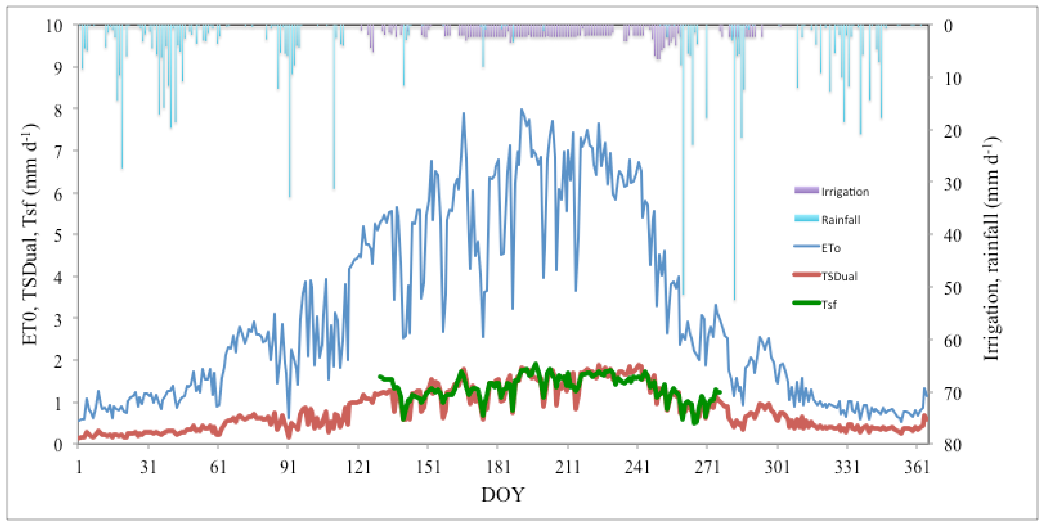

Figure 3.
Crop transpiration modeled with STSEB (TSTSEB) and measured with sap flow (Tsf) in 2014.

Figure 4.
Crop evapotranspiration (ETcSDual), transpiration (TSDual), and soil evaporation (EsSDual) modeled with SIMDualKc for 2014.
Figure 4.
Crop evapotranspiration (ETcSDual), transpiration (TSDual), and soil evaporation (EsSDual) modeled with SIMDualKc for 2014.
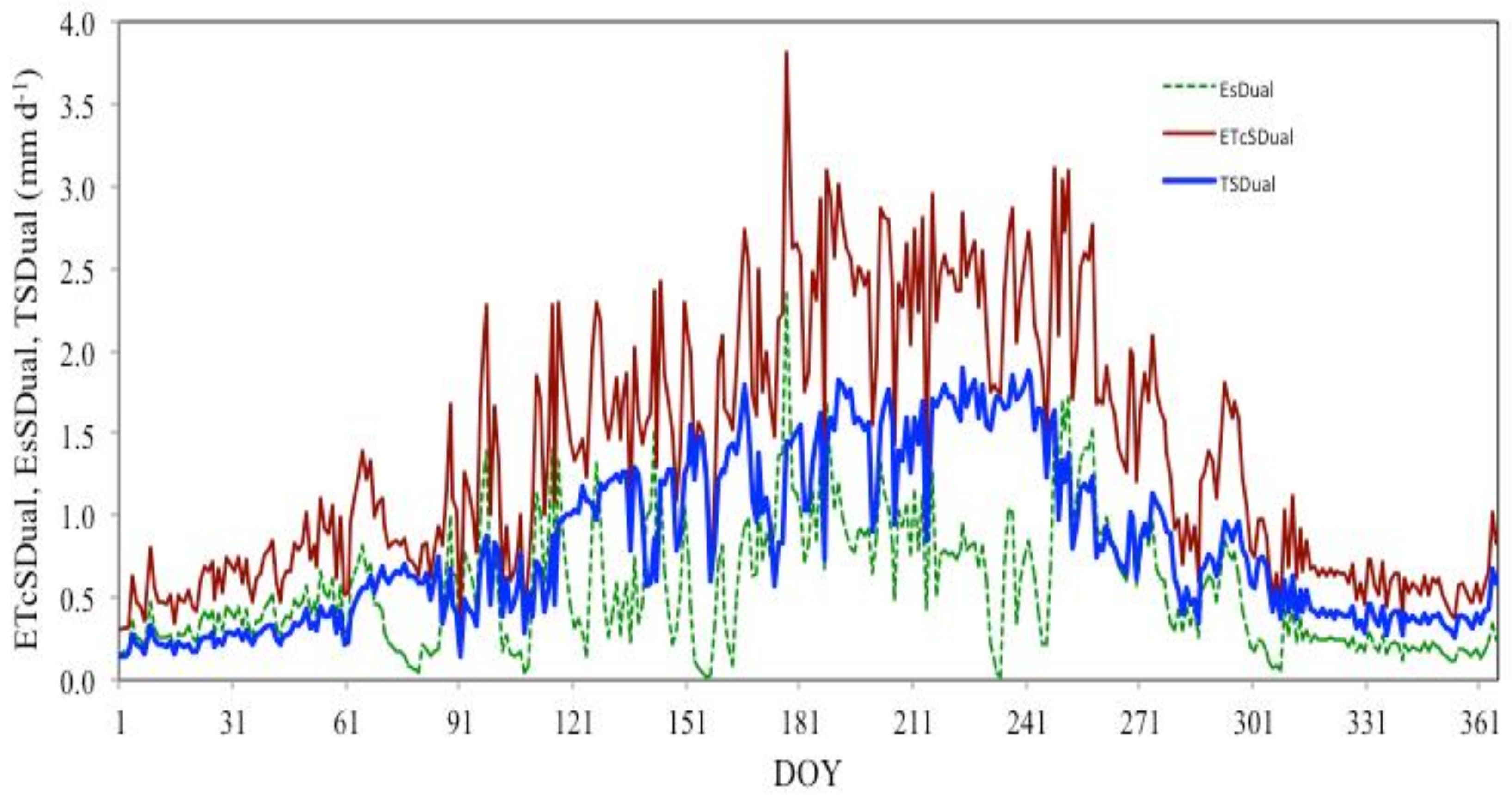
Figure 5.
Crop evapotranspiration (ETcSTSEB), transpiration (TSTSEB), and soil evaporation (EsSTSEB) modeled with STSEB for 2014.
Figure 5.
Crop evapotranspiration (ETcSTSEB), transpiration (TSTSEB), and soil evaporation (EsSTSEB) modeled with STSEB for 2014.
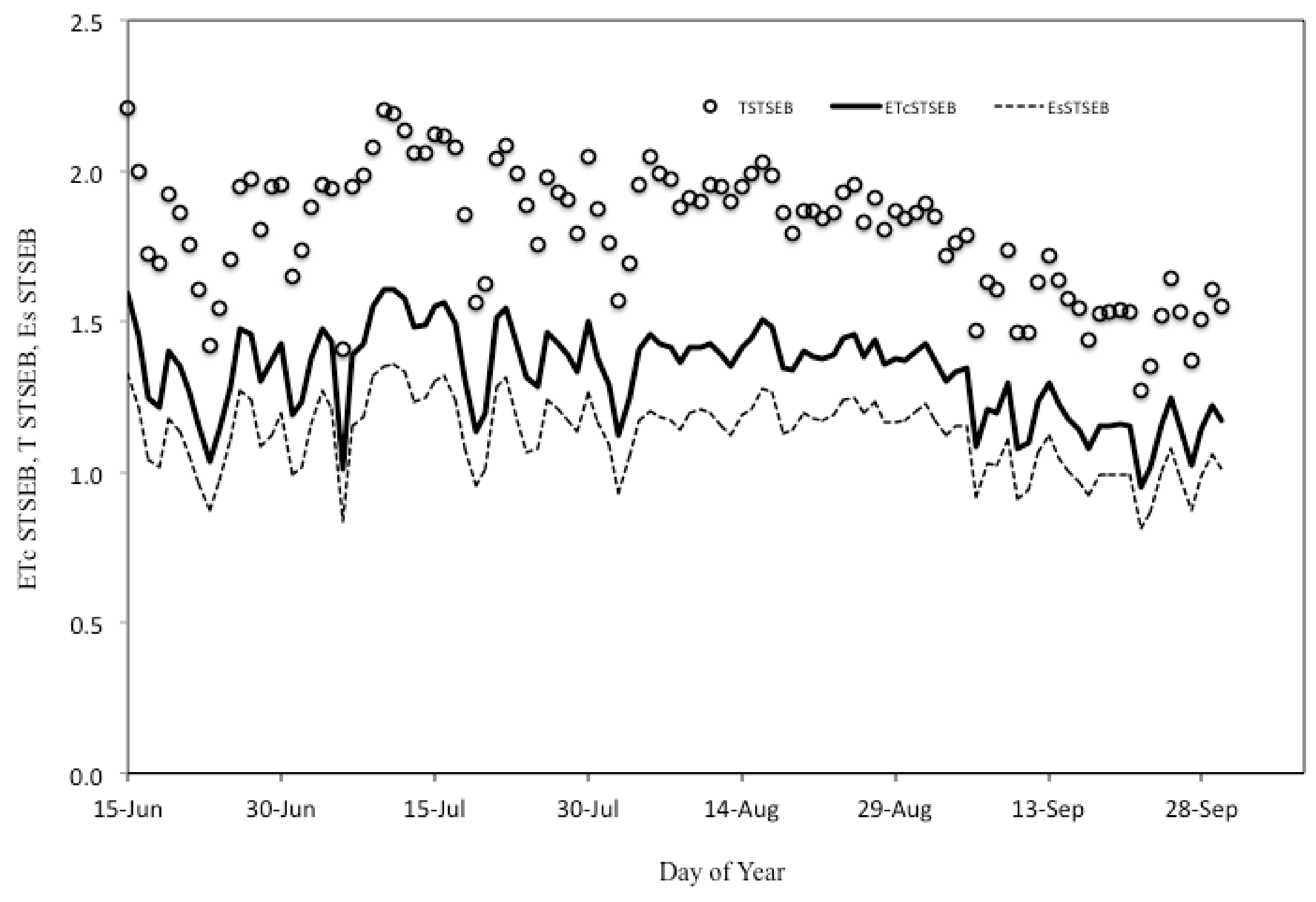
Figure 6.
Comparing actual evapotranspiration (ETcSDual), transpiration (TcSDual), and soil evaporation (EsSDual) modeled with SIMDualKc with STSEB modeled evapotranspiration (ETcSTSEB), transpiration (TSTSEB), and soil evaporation (EsSTSEB) for 2014 (DOY 130 to 276). Plotted values are in mm d−1.
Figure 6.
Comparing actual evapotranspiration (ETcSDual), transpiration (TcSDual), and soil evaporation (EsSDual) modeled with SIMDualKc with STSEB modeled evapotranspiration (ETcSTSEB), transpiration (TSTSEB), and soil evaporation (EsSTSEB) for 2014 (DOY 130 to 276). Plotted values are in mm d−1.

Table 1.
Summary of the monthly values of maximum and minimum temperatures (°C), rainfall (mm month−1), and reference evapotranspiration (mm month−1) for the two study years.
Table 1.
Summary of the monthly values of maximum and minimum temperatures (°C), rainfall (mm month−1), and reference evapotranspiration (mm month−1) for the two study years.
| Mean Maximum Temperature (°C) | Mean Mimimum Temperature (°C) | Rainfall (mm Month−1) | ETo (mm Month−1) | |||||
|---|---|---|---|---|---|---|---|---|
| Month | 2013 | 2014 | 2013 | 2014 | 2013 | 2014 | 2013 | 2014 |
| January | 15.2 | 14.9 | 6.3 | 6.8 | 89.9 | 102.2 | 28.4 | 31.9 |
| February | 14.8 | 14.5 | 3.8 | 5.6 | 48.9 | 148.0 | 42.5 | 35.0 |
| March | 16.2 | 18.5 | 7.9 | 5.9 | 240 | 40.1 | 51.5 | 80.9 |
| April | 20.8 | 21.3 | 7.7 | 9.7 | 26.2 | 119.1 | 99.9 | 82.3 |
| May | 24.6 | 25.7 | 8.2 | 9.9 | 15.2 | 16.7 | 134.6 | 144.1 |
| June | 29.8 | 28.5 | 12.3 | 13.1 | 13.0 | 9.4 | 167.6 | 150.7 |
| July | 33.1 | 31.5 | 15.3 | 14.3 | 0.1 | 5.5 | 175.3 | 173.8 |
| August | 35.0 | 31.7 | 15.0 | 14.6 | 0.1 | 0.0 | 176.0 | 175.2 |
| September | 31.0 | 27.7 | 14.4 | 15.6 | 55.9 | 124.1 | 125.4 | 97.8 |
| October | 24.3 | 24.8 | 12.8 | 13.9 | 159.9 | 106.3 | 83.5 | 80.1 |
| November | 16.9 | 16.8 | 5.9 | 7.7 | 8.2 | 172.8 | 52.8 | 53.5 |
| December | 15.6 | 14.3 | 4.4 | 3.7 | 79.7 | 9.0 | 43.0 | 35.0 |
Table 2.
Standard and calibrated parameters used in SIMDualKc model (p—depletion fraction, Kcb ini—basal crop coefficient for the initial crop development stage; Kcb mid—basal crop coefficient for the mid stage; Kcb end—basal crop coefficient for the end-season stage, ML parameter; TEW—total evaporable water; REW—readily evaporable water; Ze—thickness of the evaporation layer; CN—curve number; aD and bD—deep percolation parameters).
| Parameters | Initial | Calibrated |
|---|---|---|
| KcbSDual ini | 0.5 | 0.4 |
| KcbSDual mid | 0.55 | 0.3 |
| KcbSDual end | 0.5 | 0.5 |
| pini, pmid, pend | 0.5 | 0.4; 0.4; 0.5 |
| Soil evaporation parameters | ||
| REW (mm) | 9.0 | 8.0 |
| TEW (mm) | 22.0 | 22.0 |
| Ze (mm) | 0.10 | 0.10 |
| Runoff and deep percolation parameters | ||
| CN | 68 | 68 |
| aD | 235 | 235 |
| bD | 0.02 | 0.02 |
Table 3.
Goodness of fit indicators relative to SIMDualKc predicted transpiration values when compared with observed transpiration data derived from sap-flow measurements.
Table 3.
Goodness of fit indicators relative to SIMDualKc predicted transpiration values when compared with observed transpiration data derived from sap-flow measurements.
| TSDual vs. Tsf | n | b | R2 | RMSE (mm d−1) | Emax (mm d−1) | AAE (mm d−1) | ARE (%) | EF | WIA |
|---|---|---|---|---|---|---|---|---|---|
| Calibration, 2013 | 146 | 1.02 | 0.72 | 0.20 | 0.52 | 0.215 | 20.3 | 0.67 | 0.92 |
| Validation, 2014 | 146 | 0.97 | 0.81 | 0.20 | 0.55 | 0.201 | 16.0 | 0.62 | 0.92 |
n = number of observations; b = regression coefficient; R2 = determination coefficient; RMSE = root mean square error; Emax = maximum absolute error; AAE = average absolute error; ARE = average relative error; EF = modeling efficiency; WIA = index of agreement; TSDual and Tsf are for transpiration simulated with SIMDualKc and observed with sapflow, respectively.
Table 4.
Mean, maximum, and minimum values of predicted (TSDual) and observed (Tsf) olive orchard transpiration rates for calibration (2013) and validation years (2014).
Table 4.
Mean, maximum, and minimum values of predicted (TSDual) and observed (Tsf) olive orchard transpiration rates for calibration (2013) and validation years (2014).
| DOY 130 to 276 | TSDual (mm d−1) | Tsf (mm d−1) |
|---|---|---|
| Calibration year (2013) | ||
| Mean | 1.25 | 1.21 |
| Maximum | 1.79 | 1.94 |
| Minimum | 1.29 | 1.31 |
| Validation year (2014) | ||
| Mean | 1.31 | 1.35 |
| Maximum | 1.89 | 1.92 |
| Minimum | 0.58 | 0.49 |
Table 5.
Goodness of fit indicators relative to STSEB predicted transpiration values when compared with observed transpiration data derived from sap-flow measurements.
Table 5.
Goodness of fit indicators relative to STSEB predicted transpiration values when compared with observed transpiration data derived from sap-flow measurements.
| TSTSEB vs. Tsf | n | b | R2 | RMSE (mm d−1) | Emax (mm d−1) | AAE (mm d−1) | ARE (%) | EF | WIA |
|---|---|---|---|---|---|---|---|---|---|
| 2014 | 107 | 0.99 | 0.86 | 0.20 | 0.68 | 0.169 | 12.4 | 0.70 | 0.87 |
n = number of observations; b = regression coefficient; R2 = determination coefficient; RMSE = root mean square error; Emax = maximum absolute error; AAE = average absolute error; ARE = average relative error; EF = modeling efficiency; WIA = Wilmott index of agreement. TSTSEB and Tsf are for transpiration simulated with STSEB and observed with sapflow, respectively.
Table 6.
Total, mean, maximum, and minimum actual evapotranspiration (ETc), transpiration (T), and soil evaporation (Es) simulated with the SIMDualKc and STSEB models in the year 2014 during the period DOY 166 to 273.
Table 6.
Total, mean, maximum, and minimum actual evapotranspiration (ETc), transpiration (T), and soil evaporation (Es) simulated with the SIMDualKc and STSEB models in the year 2014 during the period DOY 166 to 273.
| DOY 166 to 273 (2014) | SIMDualKc | Total (mm) | STSEB | Total (mm) |
|---|---|---|---|---|
| Mean (mm d−1) | ||||
| ETc | 2.37 | 245.1 | 1.33 | 143.4 |
| T | 1.48 | 147.2 | 1.80 | 194.8 |
| Es | 0.89 | 98.0 | 1.12 | 121.4 |
| Maximum (mm d−1) | ||||
| ETc | 3.81 | 1.61 | ||
| T | 1.89 | 2.21 | ||
| Es | 2.36 | 1.36 | ||
| Minimum (mm d−1) | ||||
| ETc | 1.20 | 0.95 | ||
| T | 0.58 | 1.27 | ||
| Es | 0.02 | 0.81 |
© 2018 by the author. Licensee MDPI, Basel, Switzerland. This article is an open access article distributed under the terms and conditions of the Creative Commons Attribution (CC BY) license (http://creativecommons.org/licenses/by/4.0/).
Share and Cite
MDPI and ACS Style
Santos, F.L. Assessing Olive Evapotranspiration Partitioning from Soil Water Balance and Radiometric Soil and Canopy Temperatures. Agronomy 2018, 8, 43. https://doi.org/10.3390/agronomy8040043
AMA Style
Santos FL. Assessing Olive Evapotranspiration Partitioning from Soil Water Balance and Radiometric Soil and Canopy Temperatures. Agronomy. 2018; 8(4):43. https://doi.org/10.3390/agronomy8040043
Chicago/Turabian StyleSantos, Francisco L. 2018. "Assessing Olive Evapotranspiration Partitioning from Soil Water Balance and Radiometric Soil and Canopy Temperatures" Agronomy 8, no. 4: 43. https://doi.org/10.3390/agronomy8040043
Note that from the first issue of 2016, this journal uses article numbers instead of page numbers. See further details here.