Olive Water Use, Crop Coefficient, Yield, and Water Productivity under Two Deficit Irrigation Strategies


Departamento de Engenharia Rural, ICAAM—Instituto de Ciências Agrárias e Ambientais Mediterrânicas, Universidade de Évora, Núcleo da Mitra, Ap. 94, 7006-554 Évora, Portugal
Agronomy 2018, 8(6), 89; https://doi.org/10.3390/agronomy8060089
Submission received: 10 May 2018
/
Revised: 23 May 2018
/
Accepted: 1 June 2018
/
Published: 3 June 2018
(This article belongs to the Special Issue Innovative Approaches to Improve Crop Water Productivity under Irrigated Conditions)
Abstract
:Reports on the annual effects of deficit irrigation regimes on olive trees are critical in shedding light on their impacts on water use, yield, and water productivity in distinct olive growing climate regions of the world. From the account of a four-year experiment, the aim of this work is to add insight into such effects on olive growing in southern Portugal. We worked with trees in an intensive ‘Cobrançosa’ orchard (300 trees ha−1) under full irrigation (FI) treatment and two regulated deficit irrigation (DI) treatments designed to replace around 70% and 50% of the FI water supply, respectively. Crop transpiration (T), irrigation water use (IWU), total water use (TWU), irrigation water use efficiency (IWUE), yield (Ya), and water productivity (WP) obtained from all treatments were analyzed, as well as their crop coefficients (Kc), simulated with the SIMDualKc software application for root zone and soil water balance based on the FAO dual crop coefficients. As expected, IWUE of the 50DI treatment was the highest among treatments, with 70DI being slightly lower. Ya showed alternate bearing with an “on-off” year sequence and was consistently higher for the 70DI treatment. WP (the ratio of Ya to IWU) values for the 70DI treatment were also consistently the highest among all treatments and years. The mean simulated Kc act values for 70DI and 50DI for the initial, mid-, and end-season compared well to the FAO56 Kc for olive crops. In general, to rank the irrigation treatments, 70DI presented the highest conversion efficiency among all treatments and years, providing a suitable DI alternative for our ‘Cobrançosa’ orchard. The 50DI treatment may be an attractive DI regime to undertake under scarce farm water resources or the expansion of olive hectares under water constraints.
1. Introduction
Alentejo is the region in Portugal with the largest area devoted to olive growing, making up approximately 52% of all olive growing areas, and it is where the economic impact of olive growing is most significant [1]. In 2010, olive groves occupied approximately 162,834 hectares in Alentejo [2], and projections estimate that the olive oil national production will be of around 100,000 Mg by 2020 [3]. Such an expansion requires from farmers an acute and careful irrigation water management of their orchards, as this is a region of scarce water resources, where water plays a decisive role in agricultural development. The ever-increasing water scarcity in a climate of mild winters and hot and dry summers means that olive irrigation water use (IWU) must be optimized in order to reduce the region’s water resources demand from its main water use sector. With an annual reference evapotranspiration (ETo) of around 1200 mm, resulting in a high water demand by crops and near daily irrigation in the summer, the sustainability of olive production in the region requires improved irrigation water productivity (WP), with deficit irrigation (DI) management being advocated as a way to better yields, oil quality, and economic returns of newly commercial orchards [4,5]. In southern Portugal, mature drip-irrigated olive orchards with planting densities of around 300 trees ha−1 require between 3500 and 4000 m3 ha−1 (350 to 400 mm) to satisfy irrigation needs for full irrigation (FI) [6,7]. Applying irrigation depths smaller than those, and at variable rates in distinct periods of the crop growth cycle (regulated deficit irrigation, RDI) has been advocated [8,9,10] to enhance water productivity (WP). Water productivity can generally be quantified in physical or economic terms [11,12]. Although WP can be defined with different perspectives [13,14], relative to irrigation [15] WP refers to the ratio between the yield (Ya) and the irrigation water applied and used (IWU) by crops. Improving WP can lead to the achievement of the highest benefits from water, and hence it is viewed as a major contributor to water saving [11]. In regions where water supply is limited and farmers are frequently forced to apply DI strategies to manage their water supply, as in southern Portugal, the increase in IWUE leads to the betterment of WP.
A recommended approach for the estimation of IWU and water stress is the dual Kc-ETo methodology adopted by FAO56 [16], where for DI strategies the concept of potential crop evapotranspiration (ETc) are replaced by the ETc (ETc act), the result of a Kc act coefficient derived from a stress coefficient (Ks) and a soil evaporation coefficient Ke, i.e., Kc act = KsKcb + Ke [17,18,19]. The SIMDualKc model [7,20,21] provides such a computational structure [17,18,22]. The implementation of DI strategies also requires knowing the plant water status, preferably determined by plant-based measurement methods [5,21,23]. Aside from providing a sign indicating when to irrigate, these strategies offer valuable information on crop water stress.
The aim of this study was to evaluate the effect of two regulated deficit irrigation regimes on ETc, IWUE, Ya, WP, and Kc in “Cobrançosa” olive trees, grown in intensive orchards in southern Portugal. Deficit irrigation is compared with fully irrigated trees. Moreover, and according to the soil water conditions, the SIMDualKc model is used to obtain and adjust Kc and Kcb to plant height and density, as well as to estimate ETc.
2. Material and Methods
2.1. Experiment Location and Design
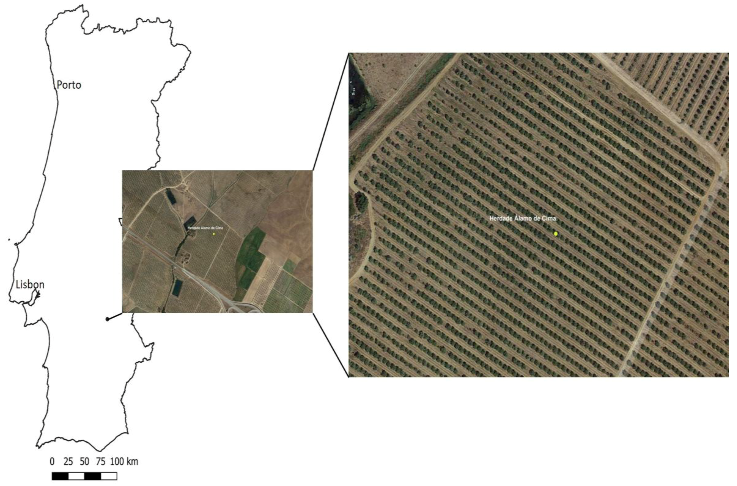
The impact of two DI scheduling regimes on ETc, IWU, IWUE, Ya, and WP for an olive orchard cv. Cobrançosa were assessed during the irrigation seasons from 2011 to 2014. The experiments were conducted at the Herdade Álamo de Cima, near Évora (38°29′49.44″ N, 7°45′8.83″ W; altitude 75 m) in southern Alentejo, Portugal. The orchard was established with 10-year old trees in grids of 4.2 m × 8.0 m (300 trees ha−1) in the East-West direction, and experiments were conducted on a shallow sandy loam Regosoil Haplic of weakly developed and unconsolidated materials [24]. The average apparent bulk soil density was 1.52 Mg m−3. The average volumetric soil water content at field capacity (i.e., at 0.03 MPa) was 0.28 m3 m−3, whereas it was 0.16 m3 m−3 at wilting point (i.e., at 1.5 MPa). Climate in the region is typically Mediterranean with long-term average annual rainfall mostly distributed from September/October to May, the remaining summer months being dry and hot. Daily values of weather data obtained from a meteorological station located at the farm and near the olive orchard were used, and daily values of ETo were calculated with the procedures prescribed in Reference [16].
In the approximately 12-hectare orchard, we applied an FI and two DI treatments. Difficulties in accurately monitoring irrigation water in the FI treatment in 2011 and a data logger short circuit in 2012 lead to this treatment being only accounted for in the years 2013 and 2014. We planned the DI strategy with two levels of irrigation to replace 70% (70DI) and 50% (50DI) of the IWU calculated for FI, based on daily ETc obtained with the single Kc approach [16,25]. Irrigation length and frequency were adjusted throughout the irrigation cycle, taking into account the crop growth and reproductive cycle, as well as rainfall events. A randomized block design with three 16.8 m × 16 m plots per treatment was used for the treatments. Each plot contained four central trees surrounded by eight border trees. All samples were taken from the central trees only. The average tree trunk diameter was 0.13 m at a height of 0.62 m from the soil surface, for an average tree height of 3.7 m. Each tree within FI plots was supplied with water by a single drip irrigation line serviced by 3.6 L h−1 emitters delivering water at a rate of 0.43 mm h−1. Emitters were spaced 1.0 m apart throughout the entire length of the emitter line placed at the soil surface and laid out along each tree row. Trees within the 70DI and 50DI plots were supplied with 2.3 and 1.6 L h−1 emitters, delivering water at rates of 0.27 and 0.19 mm h−1, respectively, and spaced 1.0 m apart in the emitter line. In general, irrigation season started in March/April and ended in September/October. Water applied (IWU) in each irrigation event was obtained by directly measuring the amount of water collected in rain gauges placed underneath selected emitters and connected to recording data loggers.
2.2. Climatic Characterization
Table 1 shows the average temperature, rainfall, and ETo for the study years. ETo for each irrigation season spanning from June to September was 861 and 718 mm in 2011 (1210 mm, annual) and 2012 (1218 mm, annual), and 878 (1233 mm, annual) and 770 mm (1209 mm, annual) in 2013 and 2014, respectively. Accordingly, on average 66% of the annual ETo encompassed the olive growth irrigation season. Total rainfall for the same irrigation period and years were 220 (662, annual), 52 (491, annual), 180 (610, annual), and 130 mm (766 mm, annual), respectively, with 2012 being the driest of all irrigation seasons. The irrigation season from June to September accounts for 23% of the total annual rainfall and 66% of the total annual ETo, making commercially irrigated olive orchards in Alentejo particularly vulnerable to climatic and water demand pressures.
2.3. Sap Flow, Stem Water Potential, Leaf Conductance, and Photosynthetically Active Radiation (PAR)
Daily tree transpiration rates on a ground area basis (mm day−1) for each irrigation treatment and year were obtained from May to the end of September or early October by continuously monitoring sap flow (Tsf) in one representative tree per plot of each treatment by the Compensation Heat Pulse method reported in Reference [26]. Heat-pulse sensors were calibrated in the laboratory on young potted trees by the water balance method, and their (ideal) velocity was corrected for probe-induced wounding effects in the trunk near the probes using coefficients, after Reference [27]. As described in Reference [4], the representative tree in the plot was selected and outfitted with two sets of heat-pulse velocity (HPV) probes and specific software was used for analysis of results [26,27]. Concerning plant water status, stem water potential (Ψst) was periodically monitored at midday with a Scholander-type pressure chamber (PMS Instruments, Corvallis, WA, USA) on two long shoots per tree, supporting five to 10 leaves in a total of eight representative samples. The detached stems from three individual trees per treatment were previously enclosed in plastic bags and reflective aluminum foil to suppress leaf transpiration, allowing leaf water potential to equilibrate with stem water potential at the point of attachment [28]; equilibration periods took about 2 h. Also, 54 midday measurements of leaf stomatal conductance (gs, mmol m−2 s−1) per treatment were taken at noon with a transient porometer (AP4, Delta-T Devices Ltd., Cambridge, UK) in three well illuminated and in three shaded leaves from the same three individual trees per treatment. Incident daily photosynthetically active radiation (PAR) and the fraction of PAR intercepted by the tree canopy were obtained from logged (CR10X, Campbell Scientific, Inc., Logan, UT, USA) measurements (umol m−2 s−1) of a set of six Quantum sensors (QPAR-02, 400–700 nm, Tranzflo, Palmerston, NT, Australia) placed in a fixed transect of three sensors on each side (North-South) of the tree line at 0.2, 1.0, and 1.88 m, respectively, and one on top of the canopy (5.0 m). Figure 1 shows the study area location in southern Portugal (a) and the intensive commercial orchard where experiments were carried out (b).
2.4. Orchard Yield, Water Use Efficiency, and Water Productivity
Trees in the central row of all plots of the three treatments were manually harvested and their fresh fruits were weighed in the field and averaged to obtain the final Ya per treatment. For each year and treatment, WP (kg m−3) [11,15] was then calculated as the ratio of final fresh fruit Ya to cumulative irrigation water supplied (IWU). IWUE per treatment was also evaluated as the ratio of tree water uptake (Tsf, mm) per treatment to IWU (mm).
2.5. ETc and Dual Kc
As mentioned above, the SIMDualKc model was used in this study. Details on soil water balance equations, adjustments to plant density and height, as well as crop water stress are given in References [17,20]. To calibrate and validate the model [17,20], and support the derivation of olive ETc act and dual Kc, the daily sap flow-based Tsf data per treatment and year was used, thus comparing T simulated by SIMDualKc (Tsim) with the observed Tsf. 70DI sap flow transpiration data (Tsf) from 2013 was used to calibrate the SIMDualKc model and validation was performed with Tsf data collected from 70DI in 2014. In the simulation, the soil evaporation (Es) was obtained in SIMDualKc. Es is an important component of ETc, especially over sparse vegetation, but difficult to measure accurately at the appropriate space-scale. It was not tested in this study. However, the goodness of the model in simulating Es was assumed as it has previously been validated for various crops, including olive crops [4,21,29,30,31], with good results. Table 2 shows the standard and calibrated parameters used in the SIMDualKc model. In the calibration and validation processes we used the methodologies described in Reference [22].
In general, the calibration of the model aimed to optimize the crop parameters Kcb and p, as well as the soil evaporation and deep percolation parameters, and the runoff curve number (CN). In the model validation process, calibrated model predictions were compared to additional and independent observed Tsf data collected in 2014. The derivation of olive dual Kc and ETc act for 70DI and 50DI in the years 2011 to 2014 were conducted after the SIMDualKc calibration and validation processes. Statistical data analysis was carried out with the software StatPlus, AnalystSoft Inc version 6 [32], and was used to assess the agreement between simulated SIMDualKc and observed values as well as their goodness of fit. Error variables are also reported.
3. Results
3.1. Water Supply, Water Use Efficiency, and Olive Transpiration
An average of 417 mm of IWU was supplied to FI (two years), for an average of 267 and 186 mm supplied to 70DI and 50DI, respectively, in the same period. Average seasonal olive Tsf was 201 mm for FI, and 190 and 163 mm for 70DI and 50DI, respectively, in the same period. Table 3 shows the seasonal values of IWU, Tsf, and ETo from 2011 to 2014.
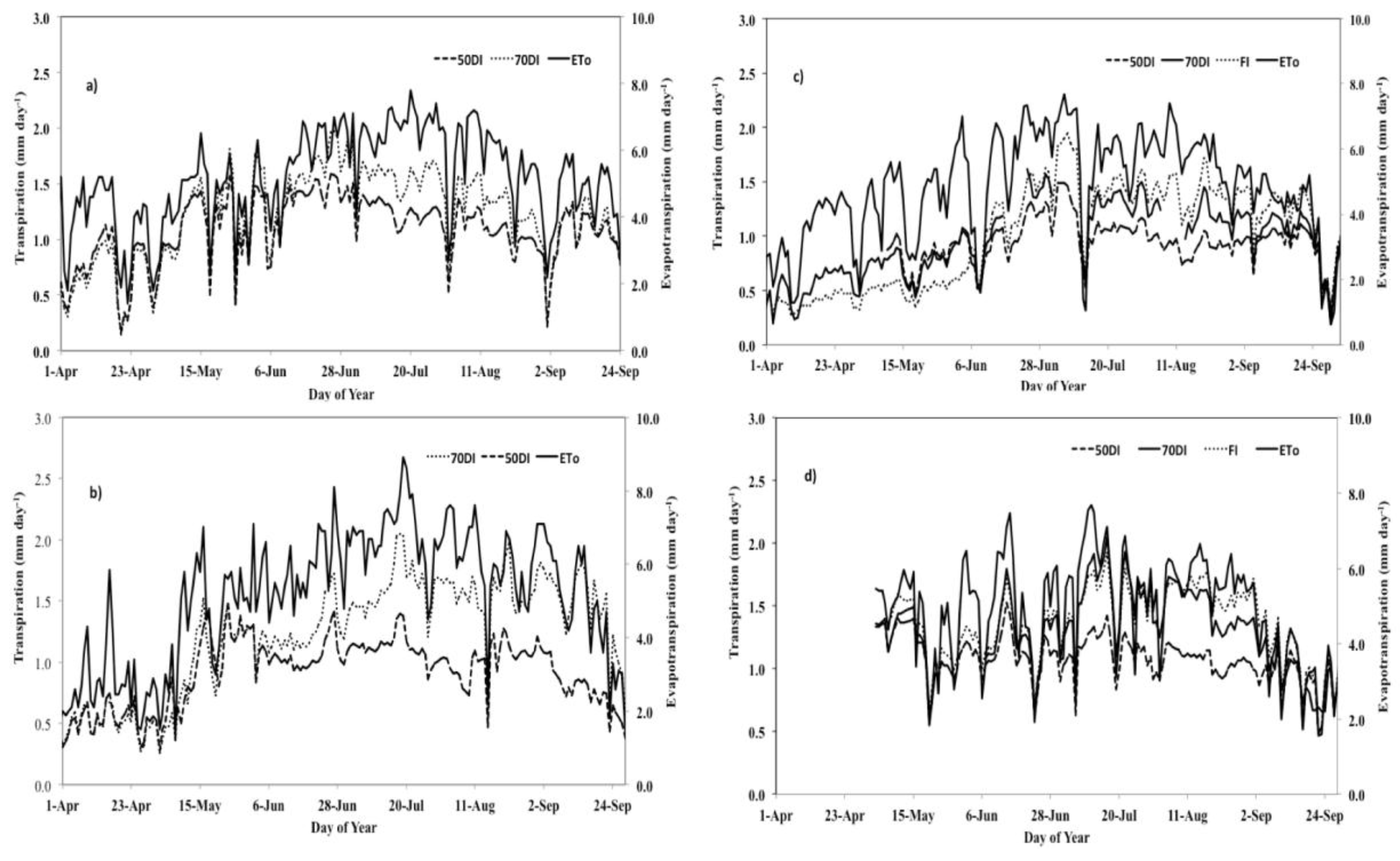
Mean daily Tsf for FI (2013 and 2014) and mean daily Tsf for 70DI and 50DI for all measured years were 1.24 ± 0.35, 1.22 ± 0.35, and 1.03 ± 0.23 mm day−1, respectively. When evaluated by their IWUE, the performance of 50DI was the highest. In 2013 and 2014, the 50DI treatment had the highest mean value of 0.88, while the corresponding value for the 70DI treatment was slightly lower, at 0.76. In the same period, the full irrigation of olive trees (FI) had the lowest IWUE, of 0.48, proving that the IWU applied was excessive. Figure 2 presents the course of daily Tsf for all treatments, as well as ETo, where differences between the day of year (DOY) recorded maximum Tsf values reflect the impacts of summer rainfall and the imposed DI treatment strategies on available soil water for olive transpiration. Their influences were most acute on 50DI in the moderate to dry summers of 2014 and 2012, respectively, when the DOY for maximum Tsf values lagged considerably behind those for FI and 70DI. Figure 2 also depicts the relative daily differences in olive water uptake (Tsf) according to the planned IWU restrictions set for each treatment.
3.2. Stomatal Leaf Conductance and Stem Water Potential
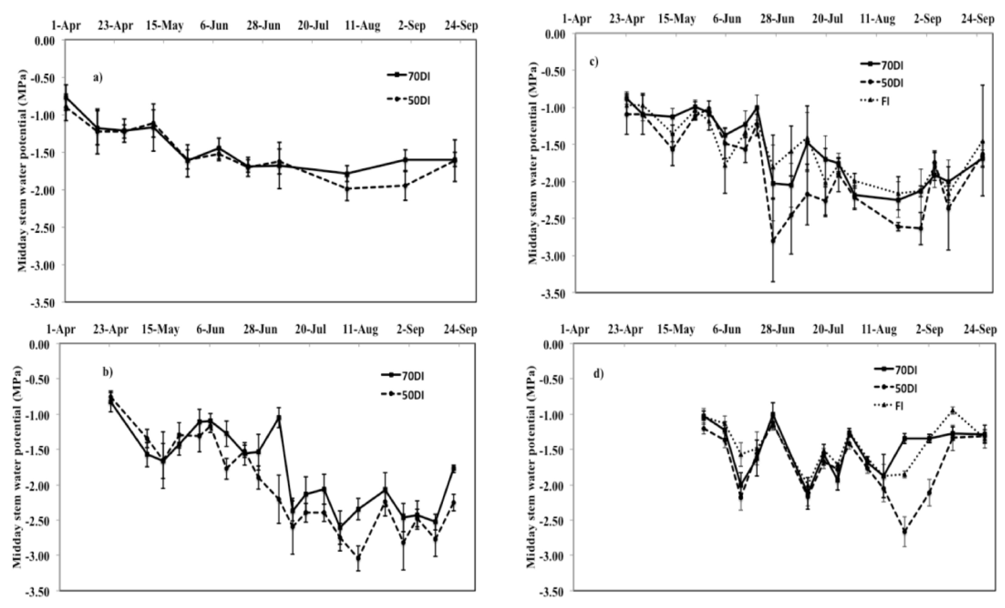
The time evolution of midday stem water potential (Ψst) for all treatments are presented in Figure 3. They provide critical tree water potential values when transpiration rates are at peak.
During the wet irrigation season of 2011, the evolution of 70DI Ψst readings (Figure 3a) until beginning of the month of August are not distinct from those of the 50DI treatment. On 6 June the stress imposed on 50DI declines Ψst readings to −1.99 MPa. The largest Ψst reading differential of −0.34 MPa among the two treatments was observed at the end of August, the driest month in the irrigation season, reflecting the effect of the lower soil water content of 50DI on leaf water status. With the first rainfall in September, both treatments quickly recovered and returned to their Ψst readings of the end of May and June. 2011 was an atypically wet year, with a total rainfall of 170 mm during the irrigation period. This helped to reduce the stress imposed on 50DI and maintained Ψs values closer to the readings obtained for 70DI.
If 2011 was wet, 2012 was an atypically dry year, with a low annual rainfall of 491 mm (long-term annual mean of around 600 mm), and 52 mm during the irrigation season, which mostly occurred in May and September with barely any rainfall from June to end of August. Reading values for Ψst (Figure 3b) of −1.01 and −1.17 MPa on 6 June for 70DI and 50DI, respectively, steadily dropped to lower values in July and August, with a slight recovery in between when mean the daily temperature and vapor pressure deficit (Da, data not shown) favored tree transpiration. With the first rains in September, and as it is expected in this Mediterranean region, both Ψst treatment readings rose to their typical pre-summer values of around −1.5 MPa. As observed in Figure 3b, 70DI readings stayed above the corresponding 50DI readings from the end of June (27 June) to mid-October (15 October), reflecting its higher IWU received during the summer months.
The more typical rainfall year of 2013 brought back expected Ψst readings for 70DI (Figure 3c), with the anticipated mild declining values from June to August and fast recovery from there onwards. For 50DI, as expected, Ψst readings declined more quickly than for 70DI and its lower value of −2.80 MPa was reached at the end of June (26 June). The first rains of September brought a quick recovery to both treatments. As for FI, Ψst readings were imperceptibly different from those of 70DI throughout the irrigation period. As seen in Figure 3c, the irrigation regime applied to FI trees provided them of needed water in crucial periods of their development growth but their Ψst readings never departed from those of 70DI, suggesting stomata closure during the dry and hot summer months of July and August even in the presence of higher water supply.
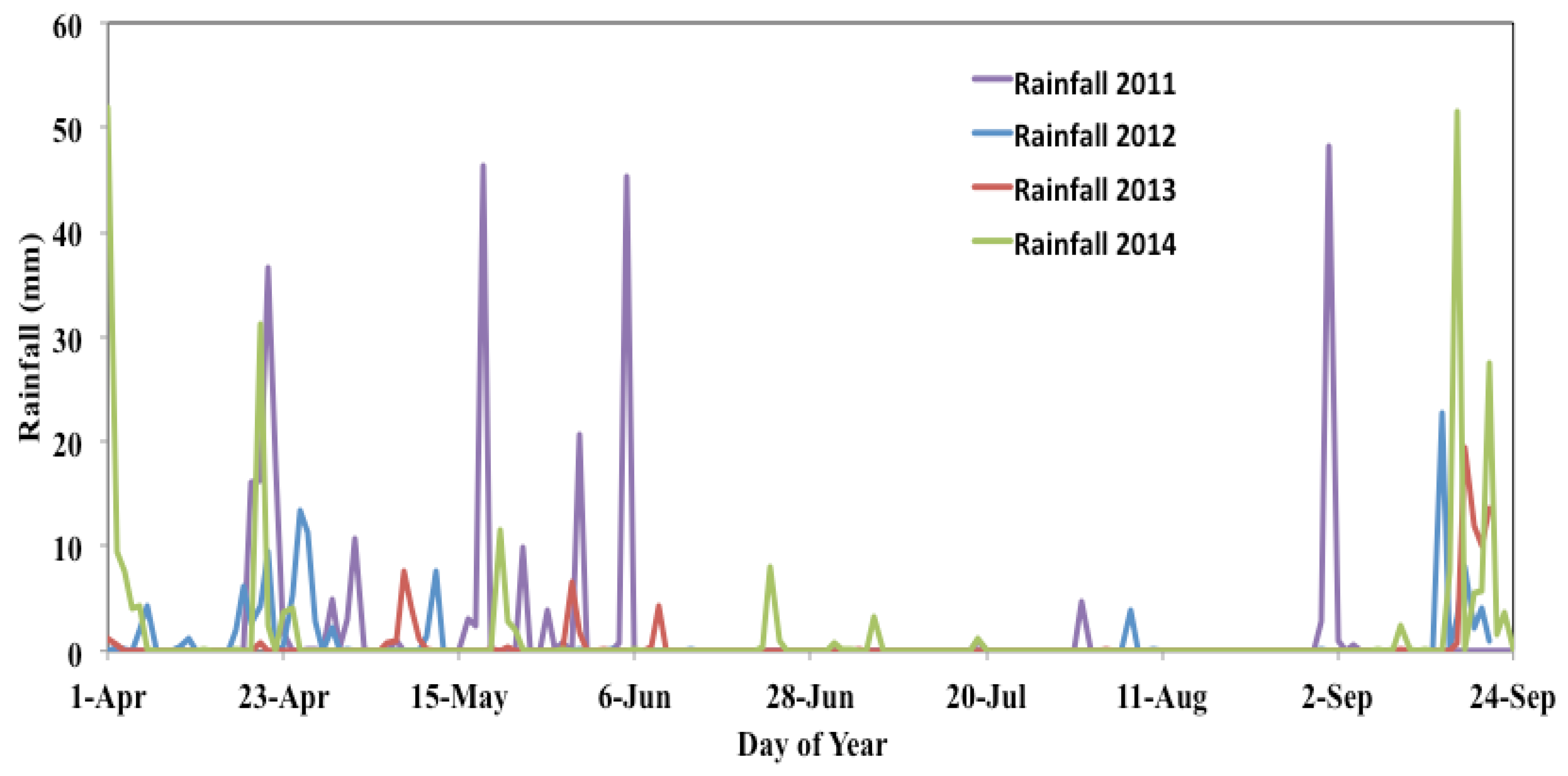
2014 was mildly wet, with 130 mm of rain falling during the irrigation season. As observed in Figure 3d, Ψst readings reflected the mild conditions until the end of July, with readings of the three treatments barely departing from each other until 6 August. The dry month of August brought a decline in Ψst readings in all treatments, with 50DI values steadily declining to its lowest value of −2.66 MPa in August (22 August), and quickly recovering in September with the first rains. Similar behavior was observed for FI and 70DI, which also saw their Ψst readings declining in August to their lowest values of −1.88 MPa in 22 August, with a quick recovery in September. Figure 4 shows the daily rainfall during the four irrigation seasons of the study.
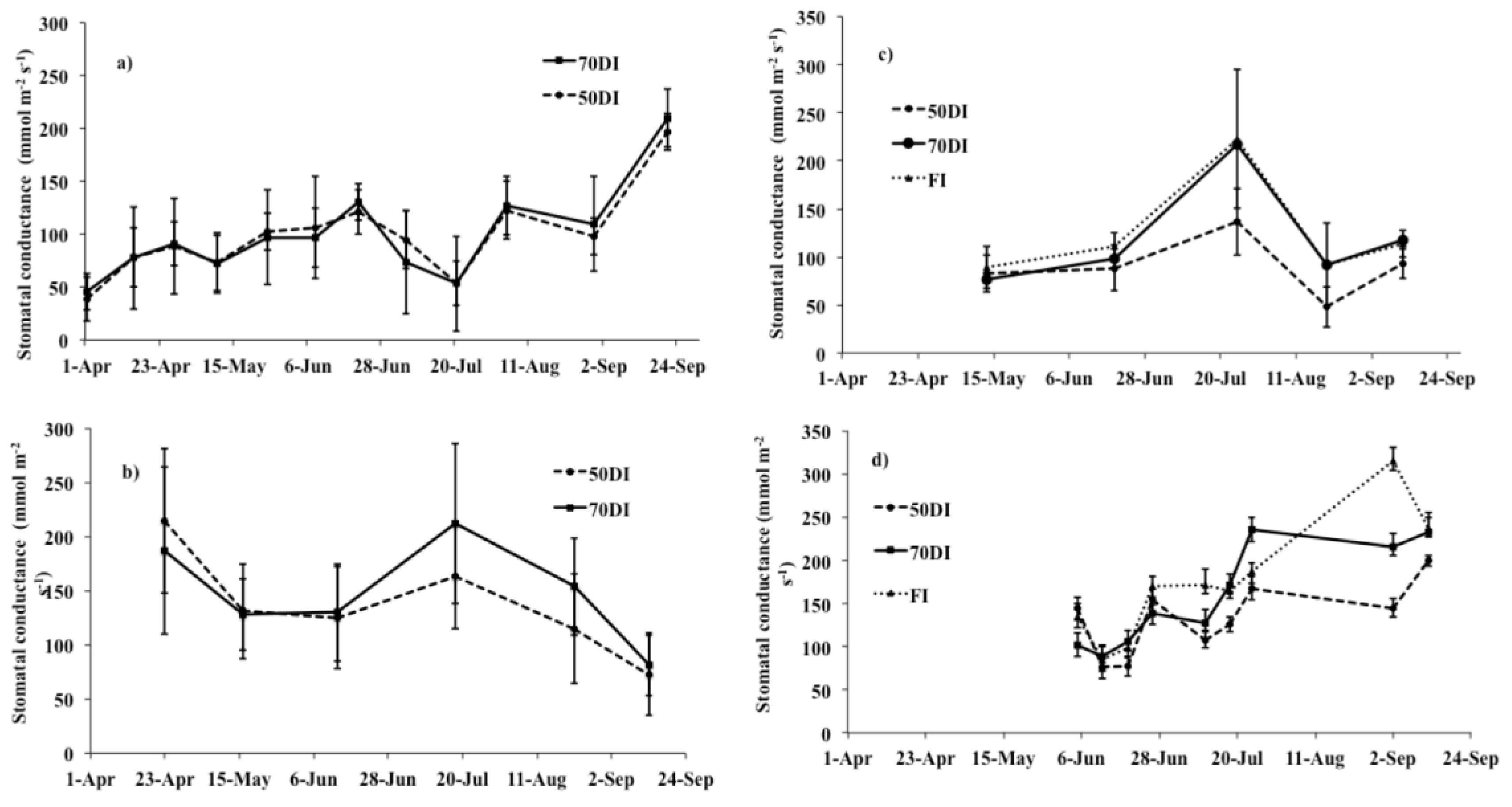
Midday stomatal leaf conductance (gs) was also influenced by the different DI regimes, as depicted in Figure 5.
In 2011 (Figure 5a), trees of 70DI and 50DI showed the same gs season trend as their counterpart Ψst readings, and displayed their lowest value of 53 mmol m−2 s−1 in 20 July. Their values slowly recovered in August, and more rapidly with the first rains at the beginning of September. In general, 70 trees showed a gs trend very similar to that observed for 50DI but with slightly higher values. In 2012 the gs values for both treatments followed the expected trend of lower readings during summer months and quick recovery in September. The higher gs value of 212 mmol m−2 s−1 was observed on 18 July, when the combination of a higher average temperature of around 30 °C and a Da of 3.4 kPa, respectively, increased transpiration and gs readings.
The gs values obtained for 2013 (Figure 5c) showed that FI exhibited practically the same gs values as 70DI throughout the irrigation season. As for 50DI, gs readings were low throughout summer. They stayed below the 70DI readings from 19 June onwards, never recovering to their gs readings until the end of September, showing that IWU and the lack of late summer rainfall deprived 50DI trees of needed water in crucial periods of the growing cycle. Furthermore, with the imposed stress their recovery was slow and never fully achieved. In the milder year of 2014, the decline of 50DI stomatal conductance was less conspicuous than that in 2013, but from 11 July onward their gs values departed from 70DI values and stayed below for most of the summer, slightly recovering in September. Regarding FI, the set of gs values obtained in 2014 (Figure 5d) showed that they match those of 70DI for most of the irrigation period, departing from them only in September, when the combination of their higher IWU and the early rainfall helped increase their values to 315 mmol m−2 s−1, but with a quick return to the same 237 mmol m−2 s−1 later in the month.
3.3. ETc and Kc
As previously stated, the SIMDualKc model was calibrated with 70DI data of 2013, and validated with 70DI data of the year 2014. The comparison of transpiration data simulated by SIMDualKc (Tsim) with observed data (Tsf) for the two years is shown in Table 4.
For the calibration year, observed and simulated transpiration data were found to be well correlated: the determination coefficient (R2 = 0.72) is high, and the root mean square error (RMSE) and average absolute error (AAE) indicators are also low, of 0.20 mm day−1, respectively. The modeling efficiency is good (EF = 0.67) and the Willmott [33] index of agreement (WIA) is high (0.92), reflecting the good correlation. In 2014, the observed (Tsf) and estimated transpiration data (Tsim) were again compared to validate the model and were found to be well correlated, with a higher determination coefficient (R2 = 0.81) and a regression coefficient b = 0.97, smaller that for the calibration year (Table 5). Overall, the goodness of fit data indicates a good performance of the model during validation, showing that the agreement between Tsim and Tsf was good. Mean Tsim and Tsf values for the calibration and validation years (10 May to 3 October, the period with available sap flow data) were very similar in 2013 (1.25 and 1.21 mm day−1, respectively) and in 2014 (1.31 and 1.35 mm day−1). Minimum mean Tsim (1.29 mm day−1) and Tsf (1.31 mm day−1) values in 2013 and in 2014 (0.58 and 0.49 mm day−1) as well as maximum Tsim (1.79 mm day−1) and Tsf (1.94 mm day−1) values in 2013 and in 2014 (1.89 and 1.92 mm day−1) were also quite close for both the calibration and validation years.
Figure 6 shows the evolution of daily crop coefficients Kcb act, Kcb, and Kc in the year 2014 for 70DI and 50DI.
For 70DI, the values were 0.24 for Kcb ini, 0.26 for Kcb mid, and 0.43 for Kcb end. A slight water stress for 70DI is shown in the graph between DOY 100 and 110, since with SIMDualKc no stress is identified when both curves of Kcb and Kcb act are coincident. Related 70DI Kc curves (Kc act, the result of the daily sum of Ke with the adjusted Kcb act) for 2014 show that the mean Kc act values were 0.51 for the initial season, 0.43 for the mid-season, and 0.67 for the end-season. These values are similar to the Kc for olive crops published by Reference [34]. Figure 6 also presents the simulated 70DI Ke curve related to soil evaporation. Initial and end-season values are on average higher, around 0.3, with mid-season showing lower values but several peaks resulting mainly from precipitation events. The year 2014 was wet, with high rainfall in April followed by more moderate events throughout July (Table 1, Figure 4). Concerning the 2014 50DI regime, Figure 6 also shows that values of Kcb act were 0.27 for Kcb ini, 0.22 for Kcb mid and 0.51 for Kcb end. Due to the low rainfall in July and August (5.5 mm) and the imposed DI regime, a water stress induced by both is shown between DOY 200 and DOY 250, since both curves of Kcb and Kcb act are not coincident. September rainfall (124 mm) and cooler weather helped to alleviate the stress. The corresponding 50DI related Kc act curves for 2014 show values of 0.54 for the initial season, 0.42 for the mid-season, and 0.76 for the end-season. These values are within the limits of Kc for olive crops, with an effective fraction of ground cover between 0.25 and 0.5 set by Reference [34]. The simulated Ke curve shows a high initial and end-season soil evaporation of around 0.3, with lower mid-season values.
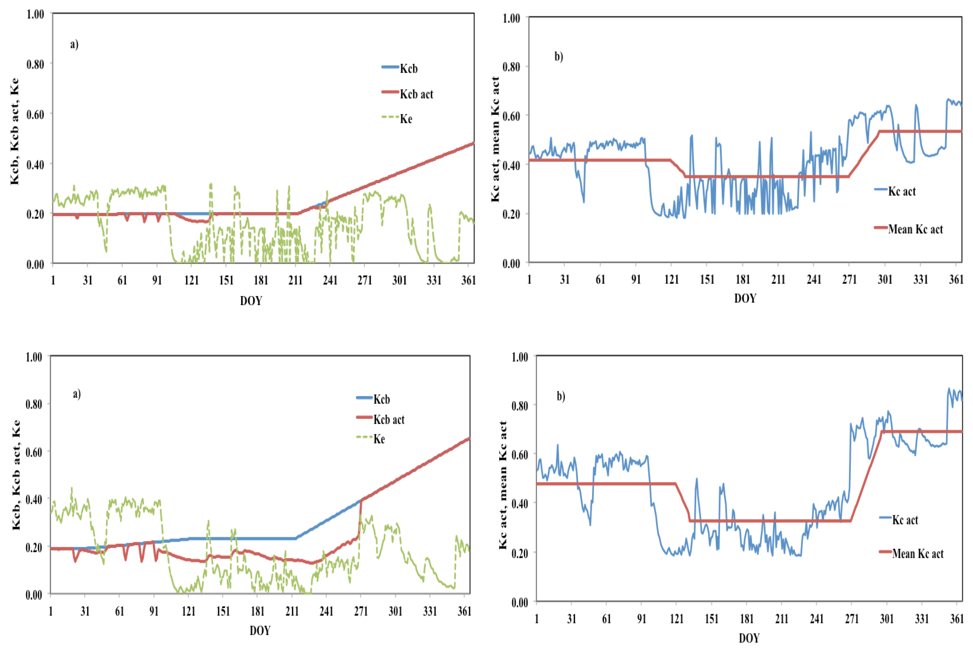
Similar curves are presented in Figure 7 that show the evolution of daily crop coefficients Kcb act, Kcb, and Kc in the year 2013 for 70DI and 50DI.
A dry summer with a cumulative rainfall of 0.2 mm in July and August (Table 1, Figure 4) and a modest rainfall in September (56 mm) added to the low IWU of the 50DI regime, resulting in a persistent water stress throughout the irrigation season as portrayed in the shape of the Kcb act curve and its departure from Kcb. Such behavior was prevented in the case of 70DI by its higher IWU regime. Table 5 summarizes the SIMDualKc annual and mean ETc act and Tsim obtained for 70DI and 50DI for all four years of the experiment, as well as the Kcb act, Ke, and Kc act obtained for the initial, mid-, and end-seasons.
Mean Kc act values in the four years of the experiment for 70DI and 50DI treatments are similar, with slightly lower values for 70DI in the initial and end-season and higher mid-season values. Similarly, mean Kcb act values in the same periods are lower for 70DI in the initial and end-season and higher in the mid-season. Mean seasonal olive Tsf for FI (Table 3), similar to the values observed for 70DI (201 mm and 200 mm, respectively), made testing for Kc values of FI with the SIMDualKc model redundant. The simulated annual and mean ETc act and Tsim values for 70DI and 50DI in the four years of the experiment are also presented in Table 5.
3.4. Ya and WP
Table 6 summarizes the obtained yield (Ya) and water productivity (WP) for all years and treatments. Olive harvest for 2012 was an exceptional “on” year, with contrasting Ya difference with the remaining years both for 70DI and 50DI. However, tree yield variability was high between all irrigated treatments and years, with bearing yields showing contrasting differences within years where an “on” year was followed by an “off” year.
On both “off” years of 2011 and 2013, respectively, 70DI yields were 41% and 50% higher than those of 50DI. In 2011 and 2013, respectively, 70DI yields were 22% and 45% higher than those of FI. Both FI and 70DI were significantly different from 50DI in 2011, with the 70DI yield being significantly different from both of the other two treatments in 2013. The “on” year of 2012 was an exceptionally higher yield year. Yields were on average higher from all treatments, with no significant differences among them. The “on” year of 2014 returned significantly different yields between 70DI and 50DI, respectively, while the FI yield was not significantly different from that of 70DI. 70DI averaged a 48% higher yield in 2014 than 50DI. In the four years, the mean 70DI yield was significantly different from those of FI and 50DI. Concerning WP, it was not significantly different for 70DI and 50DI treatments in the years 2011 and 2012, respectively. Years 2013 and 2014 brought higher and significantly different 70DI WP than either 50DI and FI, whose WP values were not significantly different between years. Accordingly, in the four years of the experiment, 70DI yielded an average of 3.0 kg of fresh fruit m−3 IWU, which was not significantly different from the 2.7 kg m−3 for 50DI. Relatively to the average amount of IWU incorporated in each unit of fresh fruit in the four years of the experiment, the results were 0.69 m3 IWU kg−1 of fresh fruit for 50DI and 0.53 m3 kg−1 for 70DI. In general, WP resulted in 5.1 and 4.7 kg of fresh fruit m−3 in the biennium 2011/2012 for 70DI and 50DI, respectively, and 3.1 and 1.9 kg m−3 of olive water uptake for 70DI and 50DI in 2013/2014, respectively. FI yielded 2.4 kg m−3 in the biennium 2013/2014.
Accounting for the total water use (TWU) in irrigation plus effective rainfall (I + R), the corresponding water productivity (WPI+R) for the 70DI treatment yielded on average 0.9 kg of fresh fruit m−3 TWU, compared to 0.7 kg m−3 for 50DI in the four years of treatment.
4. Discussion
For our ‘Cobrançosa’ trees grown in orchards in southern Portugal, the main aim of this study was to evaluate the effect of two deficit irrigation (DI) regimes on tree evapotranspiration (ETc), water use efficiency (IWUE), yield (Ya), and water productivity (WP). Deficit irrigation was compared with fully irrigated (FI) trees. The average irrigation water supplied to FI in 2013 and 2014 was considerably different from the FI crop water uptake in the same period. Average irrigation water supplied to 70DI and 50DI were more in harmony with their crop water consumption during the years of the experiment. The irrigation water use efficiency of 50DI was the highest among treatments, closely followed by the 70DI treatment, while FI water use efficiency lagged behind in the two last seasons of the study. Significant water savings were achieved with both DI regimes, as many authors have reported [9,35]. As for us, water savings by DI regimes are usually viewed as major contributors to their water productivity enhancement [11], with little impact on yield [35,36,37,38]. Also, as our data also show, many authors have reported increases in water productivity under DI regimes for olive [39,40,41,42].
Reference [37] compared deficit irrigated to fully irrigated olive trees and reported that the DI strategy reduced ETc, and consequently the yield, through an asymptotic yield-ETc function [39]. In our study, olive yields did not always increase with expanding seasonal irrigation water applied. Comparatively, and despite the larger irrigation supplies, FI used almost the same amount of water in satisfying olive seasonal consumptive use as 70DI (201 and 190 mm, respectively, in the two last seasons of the study), with no significant yield increase. Reference [5] showed similar results for cv. ‘Cordova’ low-density olive trees grown in orchards in southern Portugal. We observed alternate bearing [39,43]; in the “off” years of 2011 and 2013, the mean yield difference among treatments was significant, with 45% reduction in fruit for FI as compared to 70DI, although there was no significant mean yield difference for the “on” years. FI yield reduction in the “off” year in relation to 70DI, despite the overall similarity of their Ψst and gs readings, may be justified by FI stomata closure in the summer [37,39] and the eventual non-linear (second order) relationships mediating water use and yield [37,39,44]. For the 70DI treatments, yield significantly increased with the irrigation water applied, except in 2012, when no significant differences were found between treatments. Reductions in fruit, as compared to 70DI, were 60% and 50% for 50DI in the “off” year of 2011 and 2013, and 47% in the “on” year of 2014, in agreement with the typically Ya reported results for DI [9]. While the irrigation water use efficiency for 50DI was the highest among treatments, meaning increases in efficiency with decreasing water application, their water productivity was lower than that of 70DI. Maximizing olive irrigation water use efficiency may not necessarily be the best option here, as growers will be likely more interested in maximizing their systems conversion of water into goods and services by consequently improving water productivity [8]. The abovementioned increases in WP for 70DI and 50DI in relation to FI are more related to their water savings through better irrigation water use efficiency (lower irrigation water applied) than through yield, as the Ya averages demonstrate. However, in a region short on water resources, as in Alentejo, it is prudent to look into water productivity and irrigation water use efficiency and performances for adequately selecting DI regimes. Furthermore, it is worthwhile to recall that in the abovementioned years of 2013 and 2014, Tsf for FI and 70DI were on average almost the same (201 and 190 mm, respectively) for an irrigation water application of 417 for FI and 267 mm for 70DI, respectively, which precludes considering FI regimes for cv. ‘Cobrançosa’ olive in Alentejo.
Readings of Ψst and gs from 2011 through 2014 provided a good assessment of olive response to water stress induced by the distinct DI regimes [5,37,40] and indirectly of their expected Ya and WP [25,45]. Other authors have found similar patterns of Ψst and gs versus Ya in similar climates [25,46]; a result of the olive adaptation to drought, when trees under stress tend to control transpiration through stomatal closure [25] and the lowering of their gs readings, with subsequent decreases in net CO2 assimilation and consequently yields [46]. Concurrently, they increase their irrigation water use efficiency, as observed for the 50DI regime.
Our seasonal trend of T followed similar patterns to those of ETo, with maximum T values observed in mid-summer [25]. However, as compared to spring and autumn, ETo values increase more in mid-summer than T values, contributing to the lower observed Kcb values in July and August than before and after mid-summer [47]. In general, mean Kc act values in the four years of the experiment for 70DI followed the characteristic olive U-shape pattern described in Reference [47]. They also were similar to the FAO Kc for olive crops published by Reference [34]. Reference [48] described a Kc for olive crops of around 0.35 during summer, and an increase thereafter. References [49,50] reported similar Kc values, after adjustments for ground cover, while Reference [51] accounted for comparable Kc values for their olive experiment in northwestern Argentina (southern hemisphere). The basal mean Kcb act values in the same periods, for 70DI and 50DI, respectively, were also similar to the standard ones proposed by Reference [34] for intensive orchards such as the one in our study (≤300 trees ha−1). They were lower than Kc act, reflecting the partitioning of ETc into transpiration (T) and soil evaporation (Es). Actually, Kc act values for 70DI and 50DI, markedly influenced by soil evaporation as they integrated the seasonal evolution of ETc act values (Table 5), illustrated the importance and influence of Es in the expression of olive ETc values for olive orchards in Mediterranean climate regions [52]; in particular, they accentuated the need for a water balance simulation model to quantify Es [31,52,53] and predict ETc and Kc for drip-irrigated olive orchards in Alentejo. Despite the good results obtained in assessing tree transpiration and the derived Kc values from sap flow tree measurements, it is worth cautioning that a small number of uncalibrated sap flow probes per tree, as used in this study, is reported to lead to large flow variability (radial and azimuthal) within and between trees [54].
5. Conclusions
For our intensive orchard cv. ‘Cobrançosa’, servicing trees with FI led to increased irrigation water applications with relatively low crop water uptake, resulting in a considerably low irrigation water use efficiency as well as reduced yields and water productivity. The moderate 70DI regime allowed for adequate values of irrigation water application and efficiency, in a region of very limited available resources, and for more robust and significant yield and water productivity values. To rank the irrigated treatments in terms of water productivity, 70DI had the highest productivity, followed by 50DI. FI showed a decline in yield per amount of applied water. Ya and the related WP results seemed to indicate 70DI as the preferred DI treatment for the ‘Cobrançosa’ orchard. Also, it is worth recalling that while 50DI had on average the highest IWUE (received 28% less irrigation water than 70DI) and on average 36% lower Ya, it generated only 12% lower WP than 70DI, which makes 50DI an attractive DI regime to undertake when farm water resources are too scarce or when the expansion of olive hectares is assumed under low farm water resources. The good Kc results obtained with SIMDualKc also show that the dual Kc simulation procedure proved adequate for our olive crop under DI regimes.
Acknowledgments
This work is funded by National Funds through the FCT—Foundation for Science and Technology under the Project UID/AGR/00115/2013.
Conflicts of Interest
The author declares no conflicts of interest.
References
- INE. Instituto Nacional de Estatística. 2016. Available online: www.ine.pt/xportal/xmain?xpid=INE&xpgid=ine_main (accessed on 14 February 2016).
- Direcção Regional de Agricultura e Pescas do Alentejo. 2016. Available online: http://www.drapal.min-agricultura.pt/drapal/ (accessed on 14 February 2016).
- COI. Consejo Oleicola Inernacional. 2016. Available online: www.internationaloliveoil.org/?lang=es_ES (accessed on 14 February 2016).
- Santos, F.L.; Valverde, P.C.; Ramos, A.F.; Reis, J.L.; Castanheira, N.L. Water use and response of a dry-farmed olive orchard recently converted to irrigation. Biosyst. Eng. 2007, 98, 102–114. [Google Scholar] [CrossRef] [Green Version]
- Ramos, A.F.; Santos, F.L. Water use, transpiration, and crop coefficients for olives (cv. Cordovil), grown in orchards in Southern Portugal. Biosyst. Eng. 2009, 102, 321–333. [Google Scholar] [CrossRef] [Green Version]
- Pôças, I.; Paço, T.; Paredes, P.; Cunha, M.; Pereira, L. Estimation of actual crop coefficients using remotely sensed vegetation indices and soil water balance modelled data. Remote Sens. 2015, 7, 2373–2400. [Google Scholar] [CrossRef]
- Paço, T.A.; Pôças, I.; Cunha, M.; Silvestre, J.C.; Santos, F.L.; Paredes, P.; Pereira, L.S. Evapotranspiration and crop coefficients for a super intensive olive orchard. An application of SIMDualKc and METRIC models using ground and satellite observations. J. Hydrol. 2014, 519B, 2067–2080. [Google Scholar] [CrossRef]
- Fernández, J.E. Understanding olive adaptation to abiotic stresses as a tool to increase crop performance. Environ. Exp. Bot. 2014, 103, 158–179. [Google Scholar] [CrossRef] [Green Version]
- Fernández, J.E.; Perez-Martin, A.; Torres-Ruiz, J.M.; Cuevas, M.V.; Rodriguez-Dominguez, C.M.; Elsayed-Farag, S.; Morales-Sillero, A.; García, J.M.; Hernandez-Santana, V.; Diaz-Espejo, A. A regulated deficit irrigation strategy for hedgerow olive orchards with high plant density. Plant Soil 2013, 372, 279–295. [Google Scholar] [CrossRef] [Green Version]
- Iniesta, F.; Testi, L.; Orgaz, F.; Villalobos, F.J. The effects of regulated and continuous deficit irrigation on the water use, growth and yield of olive trees. Eur. J. Agron. 2009, 30, 258–265. [Google Scholar] [CrossRef]
- Rodrigues, G.C.; Pereira, L.S. Assessing economic impacts of deficit irrigation as related to water productivity and water costs. Biosyst. Eng. 2009, 103, 536–551. [Google Scholar] [CrossRef] [Green Version]
- Seckler, D.; Amarasinghe, U.; Molden, D.; de Silva, R.; Barker, R. World Water Demand and Supply, 1990 to 2025: Scenarios and Issues; Research Report 19; International Water Management Institute: Colombo, Sri Lanka, 1998. [Google Scholar]
- Playán, E.; Mateos, L. Modernization and optimization of irrigation systems to increase water productivity. Agric. Water Manag. 2005, 80, 100–116. [Google Scholar] [CrossRef] [Green Version]
- Molden, D.; Murray-Rust, H.; Sakthivadivel, R.; Makin, I. A water productivity framework for understanding and action. In Water Productivity in Agriculture: Limits and Opportunities for Improvement; Kijne, J.W., Barker, R., Molden, D., Eds.; CABI Publishing: Wallingford, UK, 2003; pp. 1–18. [Google Scholar]
- Pereira, L.S.; Cordery, I.; Iacovides, I. Coping with Water Scarcity: Addressing the Challenges; Springer: Dordrecht, The Netherlands, 2009. [Google Scholar]
- Allen, R.G.; Pereira, L.S.; Raes, D.; Smith, M. Crop Evapotranspiration: Guide-Lines for Computing Crop Water Requirements; Irrigation and Drainage Paper, 56; Food and Agriculture Organization (FAO): Rome, Italy, 1998. [Google Scholar]
- Santos, F.L. Assessing Olive Evapotranspiration Partitioning from Soil Water Balance and Radiometric Soil and Canopy Temperatures. Agronomy 2018, 8, 43. [Google Scholar] [CrossRef]
- Pereira, L.S.; Paredes, P.; Rodrigues, G.C.; Neves, M. Modeling malt barley water use and evapotranspiration partitioning in two contrasting rainfall years. Assessing AquaCrop and SIMDualKc models. Agric. Water Manag. 2015, 159, 239–254. [Google Scholar] [CrossRef]
- Er-Raki, S.; Chehbouni, A.; Boulet, G.; Williams, D.G. Using the dual approach of FAO-56 for partitioning ET into soil and plant components for olive orchards in a semi-arid region. Agric. Water Manag. 2010, 97, 1769–1778. [Google Scholar] [CrossRef] [Green Version]
- Rosa, R.D.; Paredes, P.; Rodrigues, G.C.; Alves, I.; Fernando, R.M.; Pereira, L.S.; Allen, R.G. Implementing the dual crop coefficient approach in interactive software. 1. Background and computational strategy. Agric. Water Manag. 2012, 103, 8–24. [Google Scholar] [CrossRef]
- Paço, T.; Ferreira, M.; Rosa, R.; Paredes, P.; Rodrigues, G.; Conceição, N.; Pacheco, C.; Pereira, L. The dual crop coefficient approach using a density factor to simulate the evapotranspiration of a peach orchard: SIMDualKc model versus eddy covariance measurements. Irrig. Sci. 2012, 30, 115–126. [Google Scholar] [CrossRef]
- Rosa, R.D.; Paredes, P.; Rodrigues, G.C.; Fernando, R.M.; Alves, I.; Pereira, L.S.; Allen, R.G. Implementing the dual crop coefficient approach in interactive software: 2. Model testing. Agric. Water Manag. 2012, 103, 62–77. [Google Scholar] [CrossRef]
- Jones, H.G. Monitoring plant and soil water status: Established and novel methods revisited and their relevance to studies of drought tolerance. J. Exp. Bot. 2007, 58, 119–130. [Google Scholar] [CrossRef] [PubMed]
- WRB. World Reference Base for Soil Resources; World Soil Resources Report 84; Food and Agriculture Organization (FAO): Rome, Italy, 2006. [Google Scholar]
- Fernández, J.E.; Green, S.R.; Caspari, H.W.; Diaz-Espejo, A.; Cuevas, M.V. The use of sap flow measurements for scheduling irrigation in olive, apple and Asian pear trees and in grapevines. Plant Soil 2008, 305, 91–104. [Google Scholar] [CrossRef]
- Green, S.R.; Clothier, B.E.; Jardine, B. Theory and practical application of heat pulse to measure sap flow. Agron. J. 2003, 95, 1371–1379. [Google Scholar] [CrossRef]
- Fernández, J.E.; Palomo, M.J.; Díaz-Espejo, A.; Clothier, B.E.; Green, S.R.; Girón, I.F.; Moreno, F. Heat-pulse measurements of sap flow in olives for automating irrigation: Tests, root flow and diagnostics of water stress. Agric. Water Manag. 2001, 51, 99–123. [Google Scholar] [CrossRef]
- Goldhamer, D.A.; Fereres, E. Simplified tree water status measurements can aid almond irrigation. Calif. Agric. 2001, 55, 32–37. [Google Scholar] [CrossRef] [Green Version]
- Wei, Z.; Paredes, P.; Liu, Y.; Chi, W.W.; Pereira, L.S. Modelling transpiration, soil evaporation and yield prediction of soybean in North China Plain. Agric. Water Manag. 2015, 147, 43–53. [Google Scholar] [CrossRef]
- Zhao, N.; Liu, Y.; Cai, J.; Paredes, P.; Rosa, R.D.; Pereira, L.S. Dual crop coefficient modeling applied to the winter wheat–summer maize crop sequence in North China Plain: Basal crop coefficients and soail evaporation component. Agric. Water Manag. 2013, 117, 93–105. [Google Scholar] [CrossRef]
- Bonachela, S.; Orgaz, F.; Villalobos, F.J.; Fereres, E. Measurement and simulation of evaporation from soil olive orchards. Irrig. Sci. 1999, 18, 205–211. [Google Scholar] [CrossRef]
- StatPlus, AnalystSoft Inc. Statistical Analysis Program for Mac OS®. Version v6. Available online: http://www.analystsoft.com/en/ (accessed on 25 October 2017).
- Willmott, C.J. On the validation of models. Phys. Geogr. 1981, 2, 184–194. [Google Scholar]
- Allen, R.G.; Pereira, L.S. Estimating crop coefficients from fraction of ground cover and height. Irrig. Sci. 2009, 28, 17–34. [Google Scholar] [CrossRef]
- García, J.M.; Cuevas, M.V.; Fernández, J.E. Production and oil quality in ‘Arbequina’ olive (Olea europaea, L.) trees under two deficit irrigation strategies. Irrig. Sci. 2013, 31, 359–370. [Google Scholar] [CrossRef]
- Fernandes-Silva, A.A.; Ferreira, T.C.; Correia, C.M.; Malheiro, A.C.; Villalobos, F.J. Influence of different irrigation regimes on crop yield and water use efficiency of olive. Plant Soil 2010, 333, 35–47. [Google Scholar] [CrossRef] [Green Version]
- Moriana, A.; Orgaz, F.; Pastor, M.; Fereres, E. Yield responses of a mature olive orchard to water deficits. J. Am. Soc. Hortic. Sci. 2003, 128, 425–431. [Google Scholar]
- Moriana, A.; Fereres, E. Plant indicator for scheduling irrigation of young olive trees. Irrig. Sci. 2002, 21, 83–90. [Google Scholar]
- Tognetti, R.; d’Andria, R.; Lavini, A.; Morelli, G. The effect of deficit irrigationon crop yield and vegetative development of Olea europaea L. (cvs. Frantoio and Leccino). Eur. J. Agron. 2006, 25, 356–364. [Google Scholar] [CrossRef]
- Tognetti, R.; d’Andria, R.; Morelli, G.; Alvino, A. The effect of deficit irrigation seasonal variations of plant water use in Olea europaea L. Plant Soil 2005, 273, 139–155. [Google Scholar] [CrossRef]
- Wahbi, S.; Wakrim, R.; Aganchich, B.; Tahi, H.; Serraj, R. Effects of partial rootzone drying (PRD) on adult olive tree (Olea europaea) in field conditions under arid climate. I. Physiological and agronomic responses. Agric. Ecosyst. Environ. 2005, 106, 289–301. [Google Scholar] [CrossRef]
- Romero, M.P.; Tovar, M.J.; Girona, J.; Motilva, M.J. Changes in the HPLC phenolic profile of virgin olive oil from young trees (Olea europaea L. cv. Arbequina) grown under different deficit irrigation strategies. J. Agric. Food Chem. 2002, 50, 5349–5354. [Google Scholar] [CrossRef] [PubMed]
- Lavee, S.; Wodner, M. The effect of yield, harvest time and fruit size on the oil content in fruits of irrigated olive trees (Olea europaea), cvs. Barnea and Manzanillo. Sci. Hortic. 2004, 99, 267–277. [Google Scholar] [CrossRef]
- Grattan, S.R.; Berenguer, M.J.; Connell, J.H.; Polito, V.S.; Vossen, P.M. Olive oil production as influenced by different quantities of applied water. Agric. Water Manag. 2006, 85, 133–140. [Google Scholar] [CrossRef]
- Boughalleb, F.; Hajlaoui, H. Physiological and anatomical changes induced by drought in two olive cultivars (cv. Zalmati and Chemlali). Acta Physiol. Plant. 2011, 33, 53–65. [Google Scholar] [CrossRef]
- Naor, A.; Schneider, D.; Ben-Gal, A.; Zipori, I.; Dag, A.; Kerem, Z.; Birger, R.; Peres, M.; Gal, Y. The effects of crop load and irrigation rate in the oil accumulation stage on oil yield and water relatiins of ‘Koroneiki’ olives. Irrig. Sci. 2013, 31, 781–791. [Google Scholar] [CrossRef]
- Testi, L.; Villalobos, F.J.; Orgaz, F.; Fereres, E. Water requirements of olive orchards—I: Simulation of daily evapotranspiration for scenario analysis. Irrig. Sci. 2006, 24, 69–76. [Google Scholar] [CrossRef]
- Villalobos, F.J.; Testi, L.; Orgaz, F.; García-Tejera, O.; Lopez-Bernal, A.; González-Dugo, M.V.; Ballester-Lurbe, C.; Castel, J.R.; Alarcón-Cabañero, J.J.; Nicolás-Nicolás, E.; et al. Modelling canopy conductance and transpiration of fruit trees in Mediterranean areas: A simplified approach. Agric. For. Meteorol. 2013, 171–172, 93–103. [Google Scholar] [CrossRef]
- Pastor, M.; Orgaz, F. Riego deficitario del olivar: Los programas de recorte de riego en olivar. Agricultura 1994, 746, 768–776. [Google Scholar]
- Orgaz, F.; Fereres, E. Riego. In El Cultivo del Olivo, 4th ed.; Barranco, D., Fernández-Escobar, R., Rallo, L., Eds.; Coedición Junta de Andalucía y Ediciones Mundi-Prensa: Madrid, España, 2004; pp. 285–306. [Google Scholar]
- Rousseaux, M.C.; Figuerola, P.I.; Correa-Tolesco, G.; Searles, P.S. Seasonal variations in sap flow and soil evaporation in an olive (Olea europaea L.) grove under two irrigation regimes in an arid region of Argentina. Agric. Water Manag. 2009, 96, 1037–1044. [Google Scholar] [CrossRef]
- Bonachela, S.; Orgaz, F.; Villalobos, F.J.; Fereres, E. Soil evaporation from drip-irrigated olive orchards. Irrig. Sci. 2001, 20, 65–71. [Google Scholar] [CrossRef]
- Ritchie, J. Model for predicting evaporation from a row crop with incomplete cover. Water Resour. Res. 1972, 8, 1204–1213. [Google Scholar] [CrossRef]
- López-Bernal, A.; Alcántara, E.; Testi, L.; Villalobos, F.J. Spatial sap flow and xylem anatomical characteristics in olive trees under different irrigation regimes. Tree Phys. 2010, 30, 1536–1544. [Google Scholar] [CrossRef] [PubMed] [Green Version]
Figure 1.
Location of the study area in southern Portugal (a) with identification of the intensive commercial olive orchard at the Herdade Álamo de Cima near Évora (38°29′49.44″ N, 7°45′8.83″ W altitude 75 m), in the Alentejo region (b).
Figure 1.
Location of the study area in southern Portugal (a) with identification of the intensive commercial olive orchard at the Herdade Álamo de Cima near Évora (38°29′49.44″ N, 7°45′8.83″ W altitude 75 m), in the Alentejo region (b).

Figure 2.
Daily evapotranspiration (ETo) and transpiration rates obtained from sap flow measurements for full irrigation (FI), 70% deficit irrigation (70DI), and 50% deficit irrigation (50DI) regimes applied to olive orchards: (a) 2011, deficit irrigation (DI) treatments; (b) 2012, DI treatments; (c) 2013, all irrigation treatments; (d) 2014, all irrigation treatments.

Figure 3.
Midday stem water potential obtained with the pressure chamber for: (a) 2011, in DI treatments; (b) 2012, in DI treatments; (c) 2013, in all irrigation treatments; (d) 2014, in all irrigation treatments.
Figure 3.
Midday stem water potential obtained with the pressure chamber for: (a) 2011, in DI treatments; (b) 2012, in DI treatments; (c) 2013, in all irrigation treatments; (d) 2014, in all irrigation treatments.

Figure 4.
Daily rainfall during the four irrigation seasons of the study, from 2011 to 2014.

Figure 5.
Leaf stomatal conductance obtained with a porometer for: (a) 2011, in DI treatments; (b) 2012, in DI treatments; (c) 2013, in all irrigation treatments; (d) 2014, in all irrigation treatments.
Figure 5.
Leaf stomatal conductance obtained with a porometer for: (a) 2011, in DI treatments; (b) 2012, in DI treatments; (c) 2013, in all irrigation treatments; (d) 2014, in all irrigation treatments.

Figure 6.
Daily crop coefficients derived from the SIMDualKc model in the year 2014 for 70DI (upper panel) and 50DI (lower panel); (a) basal crop coefficient adjusted for climate conditions and canopy density (Kcb), basal crop coefficient (Kcb act) adjusted for water stress conditions, soil evaporation coefficient (Ke); (b) actual (Kc act) and mean crop coefficient for the different growth stages.

Figure 7.
Daily crop coefficients derived from the SIMDualKc model in the year 2013 for 70DI (upper panel) and 50DI (lower panel); (a) basal crop coefficient adjusted for climate conditions and canopy density (Kcb), basal crop coefficient (Kcb act) adjusted for water stress conditions, soil evaporation coefficient (Ke); (b) actual (Kc act) and mean crop coefficient for the different growth stages.


Table 1.
Monthly average values of temperature (°C), rainfall (mm month−1), and ETo (mm month−1) in the four years of the study.
Table 1.
Monthly average values of temperature (°C), rainfall (mm month−1), and ETo (mm month−1) in the four years of the study.
| Month | Temperature (°C) | Rainfall (mm month−1) | ETo (mm month−1) | |||||||||
|---|---|---|---|---|---|---|---|---|---|---|---|---|
| 2011 | 2012 | 2013 | 2014 | 2011 | 2012 | 2013 | 2014 | 2011 | 2012 | 2013 | 2014 | |
| January | 9.2 | 8.6 | 10.8 | 10.9 | 76.1 | 15.0 | 89.9 | 102.2 | 31.7 | 36.0 | 28.4 | 31.9 |
| February | 10.4 | 7.7 | 9.3 | 10.1 | 62.5 | 0.6 | 48.9 | 148.0 | 48.5 | 60.8 | 42.5 | 35.0 |
| March | 12.0 | 13.1 | 12.1 | 12.2 | 39.3 | 27.0 | 240 | 40.1 | 72.5 | 95.7 | 51.5 | 80.9 |
| April | 17.0 | 11.9 | 14.3 | 15.5 | 97.6 | 39.1 | 26.2 | 119.1 | 110.8 | 81.8 | 99.9 | 82.3 |
| May | 19.8 | 18.7 | 16.4 | 17.8 | 99.0 | 44.1 | 15.2 | 16.7 | 140.7 | 136.3 | 134.6 | 144.1 |
| June | 21.2 | 21.4 | 21.1 | 20.8 | 46.0 | 0.3 | 13.0 | 9.4 | 172.7 | 174.7 | 167.6 | 150.7 |
| July | 22.2 | 23.0 | 24.2 | 22.9 | 5.8 | 0.0 | 0.1 | 5.5 | 201.9 | 211.8 | 175.3 | 173.8 |
| August | 22.7 | 23.3 | 25.0 | 23.2 | 51.1 | 3.9 | 0.1 | 0.0 | 173.3 | 189.3 | 176.0 | 175.2 |
| September | 21.6 | 21.8 | 22.7 | 21.7 | 1.6 | 41.5 | 55.9 | 124.1 | 135.2 | 140.0 | 125.4 | 97.8 |
| October | 19.4 | 16.8 | 18.6 | 19.4 | 56.7 | 95.1 | 159.9 | 106.3 | 103.2 | 76.2 | 83.5 | 80.1 |
| November | 12.4 | 11.8 | 11.4 | 12.3 | 129.2 | 229.2 | 8.2 | 172.8 | 42.0 | 34.0 | 52.8 | 53.5 |
| December | 9.1 | 10.1 | 10.0 | 9.0 | 12.5 | 71.9 | 79.7 | 9.0 | 28.3 | 23.6 | 43.0 | 35.0 |
Table 2.
Standard and calibrated parameters used in SIMDualKc model (p, depletion fraction, Kcb ini, basal crop coefficient for the initial crop development stage, Kcb mid, basal crop coefficient for the mid-season stage, Kcb end, basal crop coefficient for the end-season stage, TEW, total evaporable water, REW, readily evaporable water, Ze, thickness of the evaporation layer, CN, curve number, aD and bD, deep percolation parameters).
| Parameters | Initial | Calibrated |
|---|---|---|
| KcbSDual ini | 0.5 | 0.4 |
| KcbSDual mid | 0.55 | 0.3 |
| KcbSDual end | 0.5 | 0.5 |
| pini, pmid, pend | 0.5 | 0.4; 0.4; 0.5 |
| Soil evaporation parameters | ||
| REW (mm) | 9.0 | 8.0 |
| TEW (mm) | 22.0 | 22.0 |
| Ze (mm) | 0.10 | 0.10 |
| Runoff and deep percolation parameters | ||
| CN | 68 | 68 |
| aD | 235 | 235 |
| bD | 0.02 | 0.02 |
Table 3.
Summary of seasonal irrigation water use (IWU), sap flow transpiration (Tsf), and reference evapotranspiration (ETo) recorded values for full irrigation (FI), 70% deficit irrigation (70DI), and 50% deficit irrigation (50DI) regimes applied to olive orchards from 2011 to 2014.
Table 3.
Summary of seasonal irrigation water use (IWU), sap flow transpiration (Tsf), and reference evapotranspiration (ETo) recorded values for full irrigation (FI), 70% deficit irrigation (70DI), and 50% deficit irrigation (50DI) regimes applied to olive orchards from 2011 to 2014.
| Year | IWU (mm) | Tsf (mm) | ETo (mm) | ||||
|---|---|---|---|---|---|---|---|
| FI | 70DI | 50DI | FI | 70DI | 50DI | ||
| 2011 | 254 | 202 | 233 | 207 | 861 | ||
| 2012 | 261 | 181 | 187 | 191 | 718 | ||
| 2013 | 410 | 262 | 182 | 192 | 178 | 160 | 878 |
| 2014 | 424 | 271 | 189 | 209 | 202 | 166 | 770 |
Table 4.
Goodness of fit indicators relative to SIMDualKc predicted transpiration values when compared with observed transpiration data derived from sap-flow measurements.
Table 4.
Goodness of fit indicators relative to SIMDualKc predicted transpiration values when compared with observed transpiration data derived from sap-flow measurements.
| Tsim vs. Tsf | n | b | R2 | RMSE (mm day−1) | Emax (mm day−1) | AAE (mm day−1) | ARE (%) | EF | WIA |
|---|---|---|---|---|---|---|---|---|---|
| Calibration, 2013 | 146 | 1.02 | 0.72 | 0.20 | 0.52 | 0.215 | 20.3 | 0.67 | 0.92 |
| Validation, 2014 | 146 | 0.97 | 0.81 | 0.20 | 0.55 | 0.201 | 16.0 | 0.62 | 0.92 |
n = number of observations, b = regression coefficient, R2 = determination coefficient, RMSE = root mean square error, Emax = maximum absolute error, AAE = average absolute error, ARE = average relative error, EF = modeling efficiency, WIA = Willmott index of agreement. Tsim and Tsf stand for transpiration simulated with SIMDualKc and observed with sap flow, respectively.
Table 5.
Summary of the annual and mean ETc act and Tsim obtained for 70DI and 50DI for all four years of the experiment, as well as the Kcb act, Ke, and Kc act obtained for the initial, mid-, and end-seasons.
Table 5.
Summary of the annual and mean ETc act and Tsim obtained for 70DI and 50DI for all four years of the experiment, as well as the Kcb act, Ke, and Kc act obtained for the initial, mid-, and end-seasons.
| Year | 70DI | |||||||||
| Kcb act | Kc act | ETc act | Tsim | |||||||
| ini | mid | end | ini | mid | end | mm | mm day−1 | mm | mm day−1 | |
| 2014 | 0.24 | 0.26 | 0.43 | 0.51 | 0.43 | 0.67 | 501 | 1.37 | 297 | 0.82 |
| 2013 | 0.19 | 0.22 | 0.40 | 0.42 | 0.35 | 0.54 | 432 | 1.18 | 277 | 0.76 |
| 2012 | 0.36 | 0.26 | 0.40 | 0.47 | 0.41 | 0.65 | 553 | 1.51 | 367 | 1.00 |
| 2011 | 0.44 | 0.25 | 0.29 | 0.61 | 0.41 | 0.55 | 579 | 1.59 | 367 | 1.00 |
| Mean | 0.31 | 0.25 | 0.38 | 0.50 | 0.40 | 0.60 | 516 | 1.41 | 327 | 0.90 |
| Year | 50DI | |||||||||
| Kcb act | Kc act | ETc act | Tsim | |||||||
| ini | mid | end | ini | mid | end | mm | mm day−1 | mm | mm day−1 | |
| 2014 | 0.27 | 0.22 | 0.51 | 0.54 | 0.42 | 0.76 | 498 | 1.38 | 271 | 0.74 |
| 2013 | 0.18 | 0.18 | 0.54 | 0.48 | 0.33 | 0.69 | 428 | 1.17 | 242 | 0.66 |
| 2012 | 0.45 | 0.17 | 0.26 | 0.56 | 0.37 | 0.58 | 526 | 1.43 | 297 | 0.81 |
| 2011 | 0.45 | 0.19 | 0.32 | 0.52 | 0.35 | 0.63 | 560 | 1.55 | 295 | 0.80 |
| Mean | 0.34 | 0.19 | 0.41 | 0.53 | 0.37 | 0.67 | 503 | 1.38 | 276 | 0.75 |
Table 6.
Summary of yield (Ya) and water productivity (WP) obtained for all years and treatments.
| Yield, Ya (Mg ha−1) | Water Productivity, WP (kg m−3 IWU) | ||||||||||
|---|---|---|---|---|---|---|---|---|---|---|---|
| 2011 | 2012 | 2013 | 2014 | Mean | 2011 | 2012 | Mean | 2013 | 2014 | Mean | |
| FI | 2.1 ± 0.8 a | 14.4 ± 2.5 a | 2.1 ± 0.7a a | 7.9 ± 2.8 a | 6.0 ± 1.8 a | - | - | - | 0.51 a | 1.85 a | 1.18 a |
| 70DI | 2.7 ± 1.5 a | 16.6 ± 2.6 a | 3.8 ± 2.0 b | 8.1 ± 2.4 a | 7.8 ± 2.1 b | 1.08 a | 6.37 a | 3.73 a | 1.43 b | 3.00 b | 2.22 b |
| 50DI | 1.6 ± 1.0 b | 12.2 ± 3.9 a | 1.9 ± 1.6 a | 4.2 ± 3.5 b | 5.0 ± 2.5 a | 0.81 a | 6.73 a | 3.77 a | 1.06 a | 2.22 a | 1.64 a |
a Treatments with the same letter in the same column are not significantly different by the Tukey test at p ≤ 0.05.
© 2018 by the author. Licensee MDPI, Basel, Switzerland. This article is an open access article distributed under the terms and conditions of the Creative Commons Attribution (CC BY) license (http://creativecommons.org/licenses/by/4.0/).
Share and Cite
MDPI and ACS Style
Santos, F.L. Olive Water Use, Crop Coefficient, Yield, and Water Productivity under Two Deficit Irrigation Strategies. Agronomy 2018, 8, 89. https://doi.org/10.3390/agronomy8060089
AMA Style
Santos FL. Olive Water Use, Crop Coefficient, Yield, and Water Productivity under Two Deficit Irrigation Strategies. Agronomy. 2018; 8(6):89. https://doi.org/10.3390/agronomy8060089
Chicago/Turabian StyleSantos, Francisco L. 2018. "Olive Water Use, Crop Coefficient, Yield, and Water Productivity under Two Deficit Irrigation Strategies" Agronomy 8, no. 6: 89. https://doi.org/10.3390/agronomy8060089
Note that from the first issue of 2016, this journal uses article numbers instead of page numbers. See further details here.