Next Generation Sequence Analysis and Computational Genomics Using Graphical Pipeline Workflows

Abstract
:
1. Review of the Current Methodologies and Tools for NGS DNA-Sequencing Data Analysis

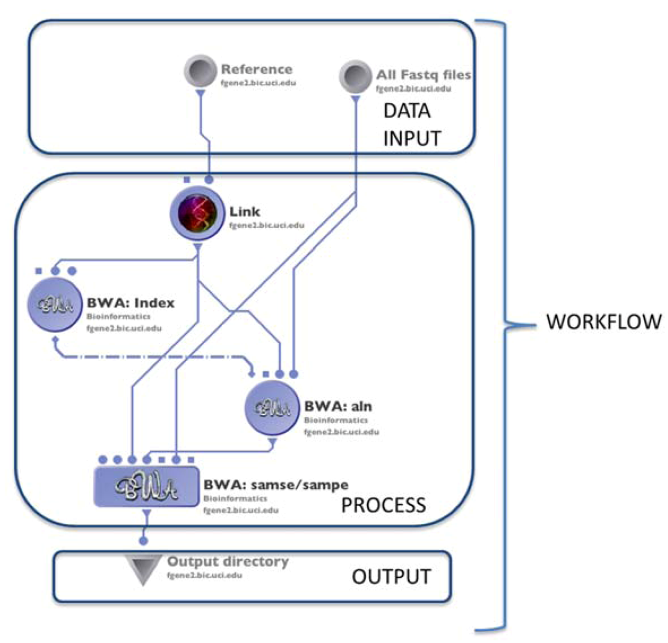
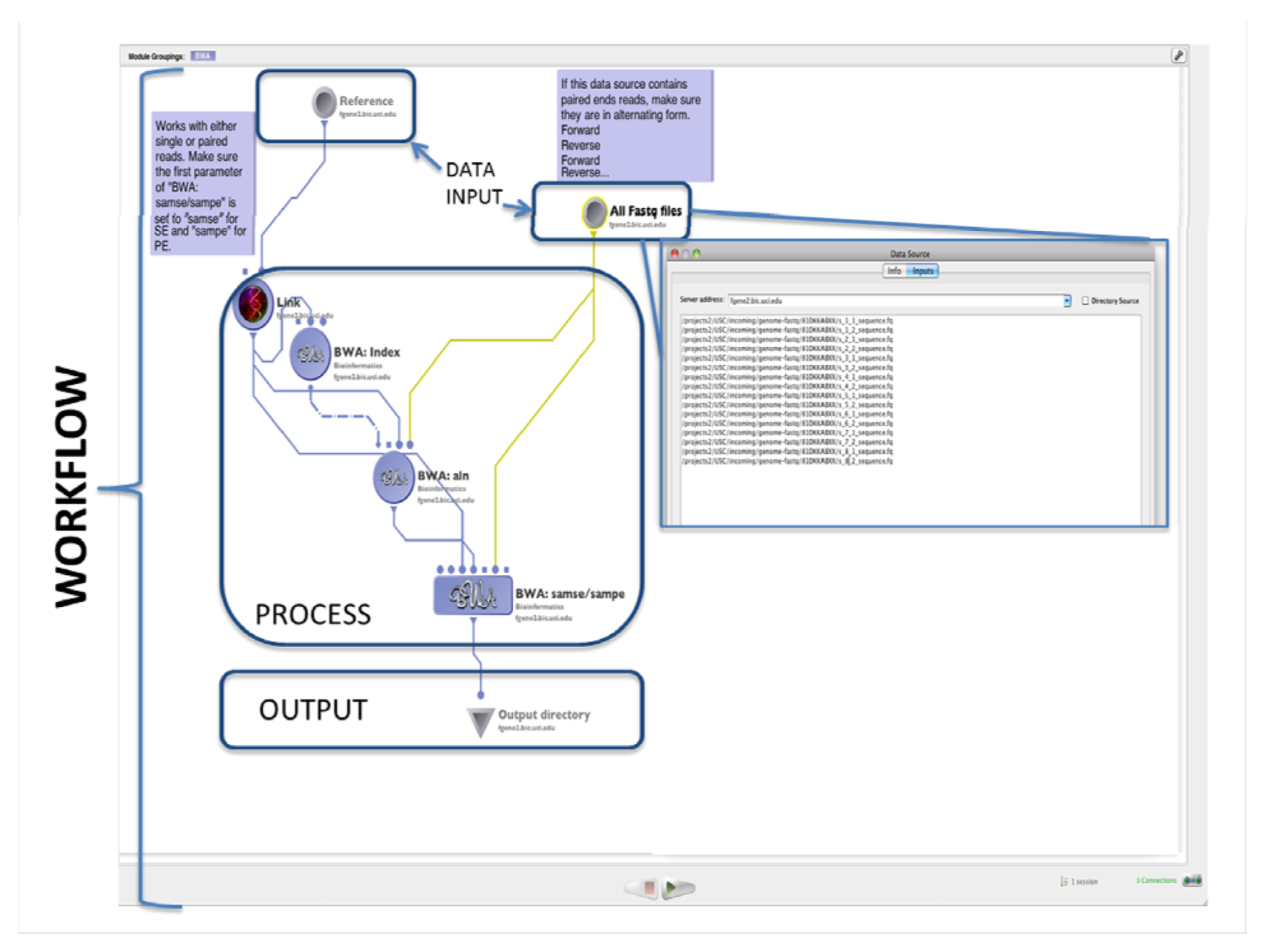
1.1. Alignment
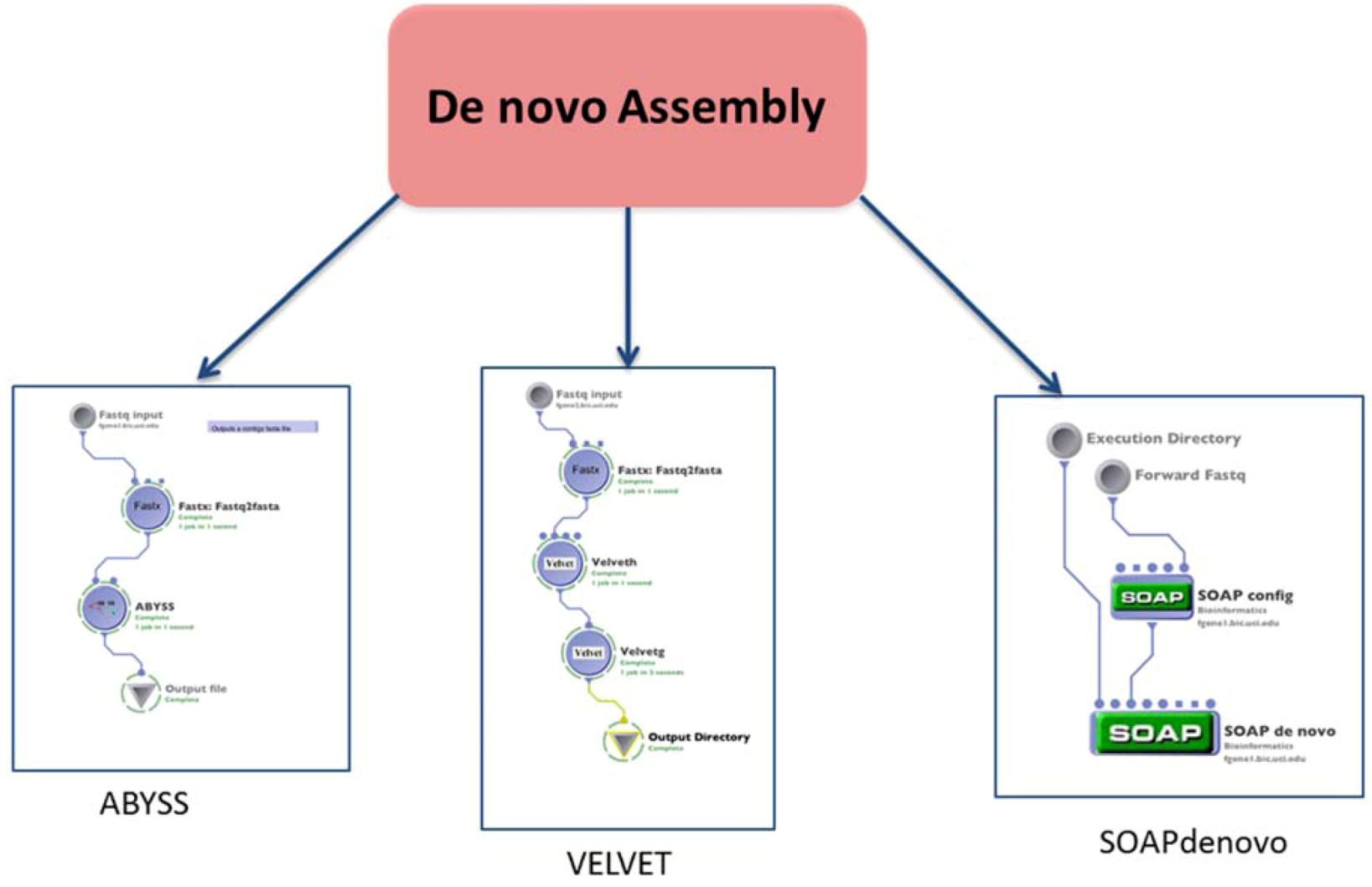
1.2. Assembly
1.3. Quality Control Improvement of Reads
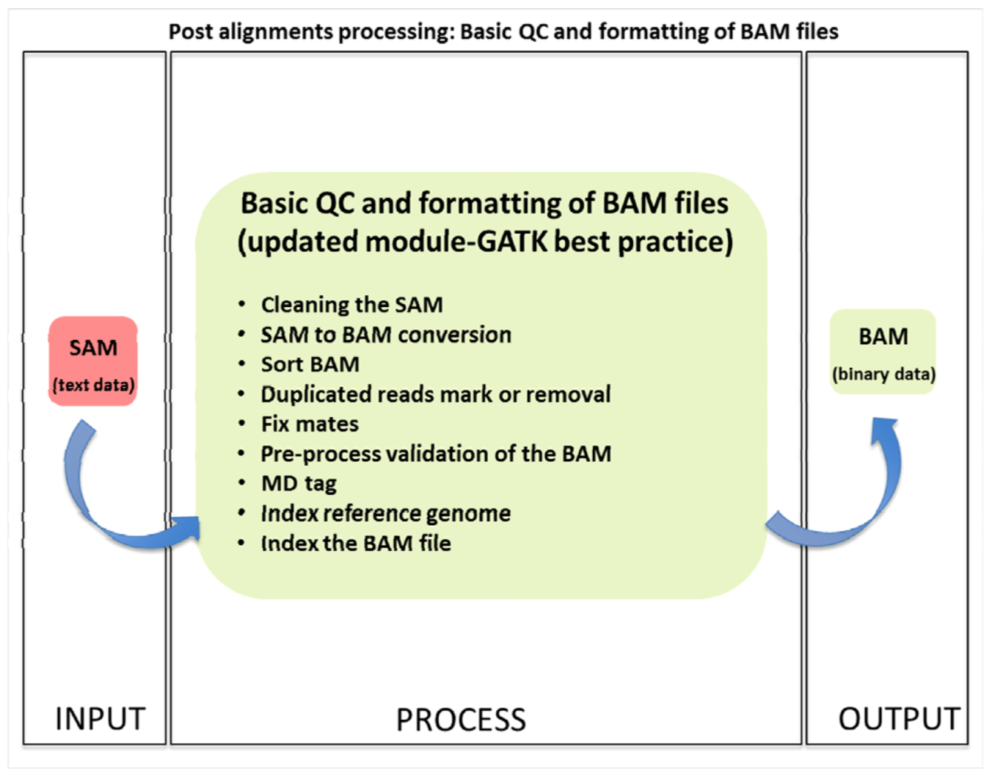
1.3.1. Basic Quality Control and File Formatting
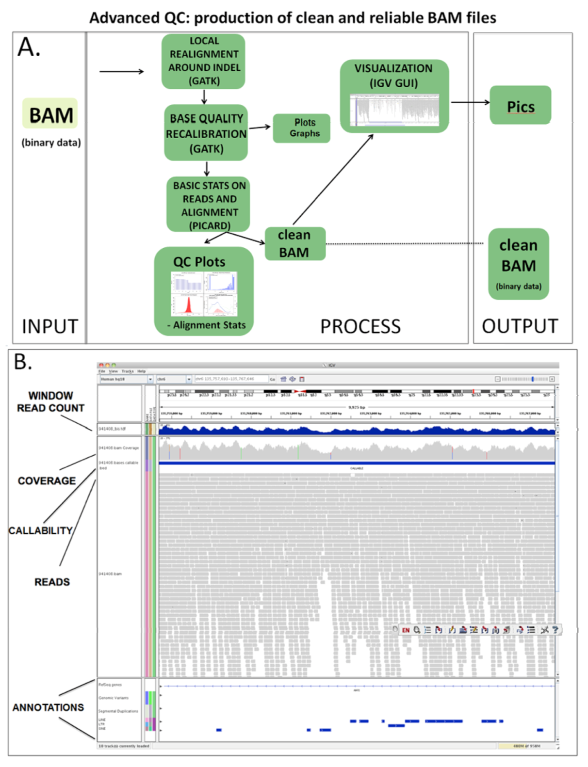
1.3.2. Advanced QC
1.4. Variant Calling and Annotation
1.4.1. SNPs and Indels Calling and Annotation
1.4.2. CNVs Calling
1.5. Statistical and Variant Prioritization Analysis
1.6. Graphical Workflows
| Workflow Management System | Module concatenation and interoperability | Asynchronous Task Management | Requires Tool Recompiling | Data Storage | Platform Independent | Client-Server Model | Grid Enabled |
|---|---|---|---|---|---|---|---|
| LONI Pipeline [57] | Y | Y | N | External | Y | Y | Y |
| pipeline.loni.ucla.edu | |||||||
| Taverna [61] | Y | N | Y | Internal(MIR) | Y | N | Y |
| taverna.sourceforge.net | |||||||
| Kepler [54] | Y | N | Y | Internal(actors) | Y | N | Y |
| kepler-project.org | |||||||
| Triana [66] | Y | N | Y | Internal data structure | Y | N | Y |
| trianacode.org | |||||||
| Workflow Navigation System [67] | N | N | N/A | External | Y | N | N |
| wns.nig.ac.jp | |||||||
| Galaxy [55] | N | N | Y | External | N | Y | N |
| usegalaxy.org | |||||||
| VisTrails [55] | Y | N | Y | Internal | N | N | N |
| www.vistrails.org |
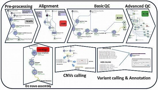
2. Description of the GPCG

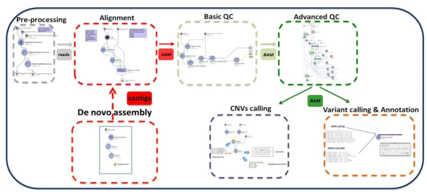
| Process | Process Description | Software & Algorithms | Input * | Output (Files) | Upstream Module Dependencies | Downstream Module Dependencies |
|---|---|---|---|---|---|---|
| Preprocessing step | Test the NGS raw data and functionality | homemade script | reads (original solexa format) | subset of reads (fastq format) | none | (1.1) Alignment, (1.2) De novo assembly |
| (1.1) Alignment | Mapping the reads to the reference genome | MAQ | reads (binary fastq format) | SAM | Preprocessing | (1.2) Basic QC |
| BWA | reads (fastq format) | SAM | ||||
| BWA-SW (SE only) | reads (solexa format) | SAM | ||||
| PERM | reads (fastq format) | SAM | ||||
| BOWTIE | reads (solexa format) | SAM | ||||
| SOAPv2 | reads (fastq format) | SAM | ||||
| MOSAIK | reads (solexa format) | SAM | ||||
| NOVOALIGN | reads (solexa format) | SAM | ||||
| (1.2) De novo assembly | Build a de novo genome sequence | VELVET | reads (fastq format) | contigs file | Preprocessing | (1.1) Alignment or none $ |
| SOAPdenovo | reads (fastq format) | contigs file | ||||
| ABYSS | reads (fastq format) | contigs file | ||||
| (1.3) Basic QC | Basic Data formatting and quality control | PICARD, SAMTOOLS | SAM | BAM | (1.1) Alignment | (1.4) Advanced QC |
| (1.4) Advanced QC | QC for advanced issues | PICARD, SAMTOOLS, GATK | BAM | BAM clean | (1.3) Basic QC | (2.1a) Variant calling (2.1b) CNV analysis |
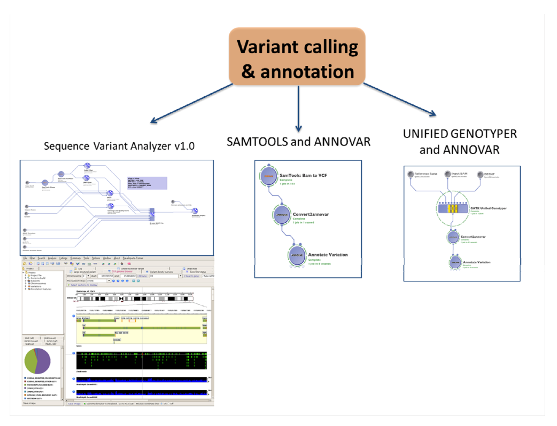
| (2.1a) Variant calling and annotation | Identify and visualize SNPs and Indels from the whole genome | Sequence Variant Analyzer v1.0 | BAM clean | csv files with variants and annotation | (1.4) Advanced QC | Statistical analysis and visualization software # |
| SAMTOOLS and ANNOVAR for annotation | BAM clean | txt files with variants | ||||
| Unified genotyper and ANNOVAR for annotation | BAM clean | txt files with variants | ||||
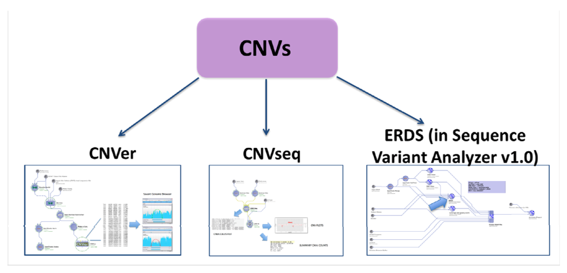
| (2.1b) CNVs calling | Analysis of CNVs (ins & del > 1 Kb) | BOWTIE CNVer SAVANT | reads (solexa format) | txt file with the CNVs calls | (1.4) Advanced QC | Statistical analysis and visualization software # |
| CNVseq | SAM | txt file with the CNVs calls | R (stat software) | |||
| SAMTOOLS ERDS Sequence variant analyzer ERDS v1.0 | BAM clean | csv file with the CNVs calls | Statistical analysis and visualization software # | |||
| Simulated data generation tool | Generate simulated reads according to the needs of the user | dwgsim | - | SE or PE .fastq files | - | (1.1) Alignment, (1.2) De novo assembly |
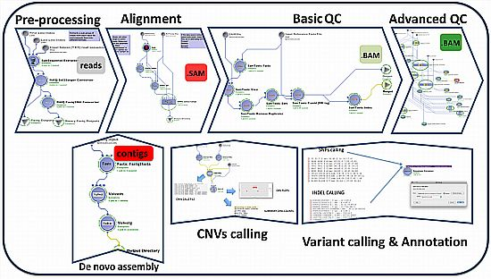
2.1. Alignment

2.2. Assembly

2.3. Quality Control Improvement of Reads
2.3.1. Basic Quality Control and File Formatting
2.3.2. Advanced QC


2.4. Variant Calling and Annotation
2.4.1. SNPs and Indels Calling and Annotation
2.4.2. CNVs Calling
2.5. Evaluation with Simulated Data
| Analytical category | Input file(file size) | Job description | GPCG workflow name | Time | Galaxy module name | Time |
|---|---|---|---|---|---|---|
| Data upload | 2.4 Gb × 2 (PE) | Upload of the data into the webserver | (N/A) | (N/A) | Upload of the data | 180 min |
| Preprocessing | 2.4 Gb fastq file | Conversion of solexa into sanger format | Preprocessing pipeline: sol2sanger | 6 min | FASTQ Groomer | 45 min |
| Alignment | 2.4 Gb × 2 fastq files (PE) | BWA paired end alignment with default parameters | BWA PE (1.1) | 132 min | Map with BWA for Illumina | 240 min |
| 2.4 G × 2 fastq files (PE) | Bowtie paired end alignment with default parameters | BOWTIE PE (1.1) | 205 min | Map with Bowtie for Illumina | 270 min | |
| Quality control (metrics and cleaning) | 1.6 Gb SAM file | Synchronization of mate-pair information | Fix Mate Information (Basic QC, 1.3) | 6 min | Paired Read Mate Fixer for paired data | 30 min |
| 1.6 Gb SAM file | Marks duplicate reads | Mark Duplicates (Basic QC, 1.3) | 2 min | Marks duplicate reads | 20 min | |
| 1.6 Gb SAM file | Reports the alignment metric of a SAM/BAM file | Collect Alignment Summary Metrics (Advanced QC, 1.4) | 2 min | SAM/BAM Alignment Summary Metrics | 6 min | |
| 1.6 Gb SAM file | Reports the SAM/BAM GCbias metrics | Collect GC Bias Metrics (Advanced QC, 1.4) | 3 min | SAM/BAM GC Bias Metrics | 7 min | |
| 1.6 Gb SAM file | Reports the insert size metrics | Collect Insert Size Metrics (Advanced QC, 1.4) | 2 min | Insertion size metrics for PAIRED data | 6 min |
2.6. Evaluation with Real Data

3. Discussion
4. Methods
4.1. The LONI Environment and Workflow Creation
4.2. Accessibility of the GPCG
4.3. Evaluation of the GPCG Workflows with Simulated and Real Data
5. Conclusions
Acknowledgments
Conflicts of Interest
References
- Dalca, A.V.; Brudno, M. Genome variation discovery with high-throughput sequencing data. Brief. Bioinform. 2010, 11, 3–14. [Google Scholar] [CrossRef]
- Alkan, C.; Coe, B.P.; Eichler, E.E. Genome structural variation discovery and genotyping. Nat. Rev. Genet. 2011, 12, 363–376. [Google Scholar] [CrossRef]
- Flicek, P.; Birney, E. Sense from sequence reads: Methods for alignment and assembly. Nat. Methods 2009, 6, S6–S12. [Google Scholar] [CrossRef]
- Pepke, S.; Wold, B.; Mortazavi, A. Computation for chip-seq and rna-seq studies. Nat. Methods 2009, 6, S22–S32. [Google Scholar] [CrossRef]
- Meaburn, E.; Schulz, R. Next generation sequencing in epigenetics: Insights and challenges. Semin. Cell Dev. Biol. 2011, 23, 192–199. [Google Scholar]
- Walsh, T.; McClellan, J.M.; McCarthy, S.E.; Addington, A.M.; Pierce, S.B.; Cooper, G.M.; Nord, A.S.; Kusenda, M.; Malhotra, D.; Bhandari, A.; et al. Rare structural variants disrupt multiple genes in neurodevelopmental pathways in schizophrenia. Science 2008, 320, 539–543. [Google Scholar]
- Rumble, S.M.; Lacroute, P.; Dalca, A.V.; Fiume, M.; Sidow, A.; Brudno, M. Shrimp: Accurate mapping of short color-space reads. PLoS Comput. Biol. 2009, 5, e1000386. [Google Scholar] [CrossRef]
- Lin, H.; Zhang, Z.; Zhang, M.Q.; Ma, B.; Li, M. Zoom! Zillions of oligos mapped. Bioinformatics 2008, 24, 2431–2437. [Google Scholar]
- Li, R.; Yu, C.; Li, Y.; Lam, T.W.; Yiu, S.M.; Kristiansen, K.; Wang, J. Soap2: An improved ultrafast tool for short read alignment. Bioinformatics 2009, 25, 1966–1967. [Google Scholar] [CrossRef]
- Chen, Y.; Souaiaia, T.; Chen, T. Perm: Efficient mapping of short sequencing reads with periodic full sensitive spaced seeds. Bioinformatics 2009, 25, 2514–2521. [Google Scholar]
- Langmead, B.; Trapnell, C.; Pop, M.; Salzberg, S.L. Ultrafast and memory-efficient alignment of short DNA sequences to the human genome. Genome Biol. 2009, 10, R25. [Google Scholar] [CrossRef]
- Li, H.; Durbin, R. Fast and accurate short read alignment with burrows-wheeler transform. Bioinformatics 2009, 25, 1754–1760. [Google Scholar] [CrossRef]
- Chen, K.; Wallis, J.W.; McLellan, M.D.; Larson, D.E.; Kalicki, J.M.; Pohl, C.S.; McGrath, S.D.; Wendl, M.C.; Zhang, Q.; Locke, D.P.; et al. Breakdancer: An algorithm for high-resolution mapping of genomic structural variation. Nat. Methods 2009, 6, 677–681. [Google Scholar]
- Olson, S.A. Emboss opens up sequence analysis. European molecular biology open software suite. Brief. Bioinform. 2002, 3, 87–91. [Google Scholar] [CrossRef]
- Myers, E.W. Toward simplifying and accurately formulating fragment assembly. J. Comput. Biol. 1995, 2, 275–290. [Google Scholar] [CrossRef]
- Pevzner, P.A.; Tang, H.; Waterman, M.S. An eulerian path approach to DNA fragment assembly. Proc. Natl. Acad. Sci. USA 2001, 98, 9748–9753. [Google Scholar] [CrossRef]
- Myers, E.W.; Sutton, G.G.; Delcher, A.L.; Dew, I.M.; Fasulo, D.P.; Flanigan, M.J.; Kravitz, S.A.; Mobarry, C.M.; Reinert, K.H.; Remington, K.A.; et al. A whole-genome assembly of drosophila. Science 2000, 287, 2196–2204. [Google Scholar]
- Jaffe, D.B.; Butler, J.; Gnerre, S.; Mauceli, E.; Lindblad-Toh, K.; Mesirov, J.P.; Zody, M.C.; Lander, E.S. Whole-genome sequence assembly for mammalian genomes: Arachne 2. Genome Res. 2003, 13, 91–96. [Google Scholar] [CrossRef]
- Zerbino, D.R.; Birney, E. Velvet: Algorithms for de novo short read assembly using de bruijn graphs. Genome Res. 2008, 18, 821–829. [Google Scholar] [CrossRef]
- Li, R.; Zhu, H.; Ruan, J.; Qian, W.; Fang, X.; Shi, Z.; Li, Y.; Li, S.; Shan, G.; Kristiansen, K.; Yang, H.; Wang, J. De novo assembly of human genomes with massively parallel short read sequencing. Genome Res. 2010, 20, 265–272. [Google Scholar]
- Simpson, J.T.; Wong, K.; Jackman, S.D.; Schein, J.E.; Jones, S.J.; Birol, I. Abyss: A parallel assembler for short read sequence data. Genome Res. 2009, 19, 1117–1123. [Google Scholar] [CrossRef]
- Miller, J.R.; Koren, S.; Sutton, G. Assembly algorithms for next-generation sequencing data. Genomics 2010, 95, 315–327. [Google Scholar]
- Ewing, B.; Green, P. Base-calling of automated sequencer traces using phred. Ii. Error probabilities. Genome Res. 1998, 8, 186–194. [Google Scholar]
- Brockman, W.; Alvarez, P.; Young, S.; Garber, M.; Giannoukos, G.; Lee, W.L.; Russ, C.; Lander, E.S.; Nusbaum, C.; Jaffe, D.B. Quality scores and snp detection in sequencing-by-synthesis systems. Genome Res. 2008, 18, 763–770. [Google Scholar] [CrossRef]
- Li, M.; Nordborg, M.; Li, L.M. Adjust quality scores from alignment and improve sequencing accuracy. Nucleic Acids Res. 2004, 32, 5183–5191. [Google Scholar]
- Li, R.; Li, Y.; Fang, X.; Yang, H.; Wang, J.; Kristiansen, K. Snp detection for massively parallel whole-genome resequencing. Genome Res. 2009, 19, 1124–1132. [Google Scholar]
- DePristo, M.A.; Banks, E.; Poplin, R.; Garimella, K.V.; Maguire, J.R.; Hartl, C.; Philippakis, A.A.; del Angel, G.; Rivas, M.A.; Hanna, M.; et al. A framework for variation discovery and genotyping using next-generation DNA sequencing data. Nat. Genet. 2011, 43, 491–498. [Google Scholar]
- Ning, Z.; Cox, A.J.; Mullikin, J.C. Ssaha: A fast search method for large DNA databases. Genome Res. 2001, 11, 1725–1729. [Google Scholar] [CrossRef]
- Martin, M.V.; Rollins, B.; Sequeira, P.A.; Mesen, A.; Byerley, W.; Stein, R.; Moon, E.A.; Akil, H.; Jones, E.G.; Watson, S.J.; et al. Exon expression in lymphoblastoid cell lines from subjects with schizophrenia before and after glucose deprivation. BMC Med. Genomics 2009, 2, 62. [Google Scholar] [CrossRef]
- Drmanac, R.; Sparks, A.B.; Callow, M.J.; Halpern, A.L.; Burns, N.L.; Kermani, B.G.; Carnevali, P.; Nazarenko, I.; Nilsen, G.B.; Yeung, G.; et al. Human genome sequencing using unchained base reads on self-assembling DNA nanoarrays. Science 2010, 327, 78–81. [Google Scholar]
- Bentley, D.R.; Balasubramanian, S.; Swerdlow, H.P.; Smith, G.P.; Milton, J.; Brown, C.G.; Hall, K.P.; Evers, D.J.; Barnes, C.L.; Bignell, H.R.; et al. Accurate whole human genome sequencing using reversible terminator chemistry. Nature 2008, 456, 53–59. [Google Scholar]
- Koboldt, D.C.; Chen, K.; Wylie, T.; Larson, D.E.; McLellan, M.D.; Mardis, E.R.; Weinstock, G.M.; Wilson, R.K.; Ding, L. Varscan: Variant detection in massively parallel sequencing of individual and pooled samples. Bioinformatics 2009, 25, 2283–2285. [Google Scholar] [CrossRef]
- Wheeler, D.A.; Srinivasan, M.; Egholm, M.; Shen, Y.; Chen, L.; McGuire, A.; He, W.; Chen, Y.J.; Makhijani, V.; Roth, G.T.; et al. The complete genome of an individual by massively parallel DNA sequencing. Nature 2008, 452, 872–876. [Google Scholar]
- Mokry, M.; Feitsma, H.; Nijman, I.J.; de Bruijn, E.; van der Zaag, P.J.; Guryev, V.; Cuppen, E. Accurate snp and mutation detection by targeted custom microarray-based genomic enrichment of short-fragment sequencing libraries. Nucleic Acids Res. 2010, 38, e116. [Google Scholar] [CrossRef]
- Shen, Y.; Wan, Z.; Coarfa, C.; Drabek, R.; Chen, L.; Ostrowski, E.A.; Liu, Y.; Weinstock, G.M.; Wheeler, D.A.; Gibbs, R.A.; et al. A snp discovery method to assess variant allele probability from next-generation resequencing data. Genome Res. 2010, 20, 273–280. [Google Scholar]
- Hoberman, R.; Dias, J.; Ge, B.; Harmsen, E.; Mayhew, M.; Verlaan, D.J.; Kwan, T.; Dewar, K.; Blanchette, M.; Pastinen, T. A probabilistic approach for snp discovery in high-throughput human resequencing data. Genome Res. 2009, 19, 1542–1552. [Google Scholar]
- Malhis, N.; Jones, S.J. High quality snp calling using illumina data at shallow coverage. Bioinformatics 2010, 26, 1029–1035. [Google Scholar] [CrossRef]
- Handsaker, R.E.; Korn, J.M.; Nemesh, J.; McCarroll, S.A. Discovery and genotyping of genome structural polymorphism by sequencing on a population scale. Nat. Genet. 2011, 43, 269–276. [Google Scholar] [CrossRef]
- Kim, J.; Sinha, S. Indelign: A probabilistic framework for annotation of insertions and deletions in a multiple alignment. Bioinformatics 2007, 23, 289–297. [Google Scholar] [CrossRef]
- Li, H.; Ruan, J.; Durbin, R. Mapping short DNA sequencing reads and calling variants using mapping quality scores. Genome Res. 2008, 18, 1851–1858. [Google Scholar] [CrossRef]
- Hormozdiari, F.; Alkan, C.; Eichler, E.E.; Sahinalp, S.C. Combinatorial algorithms for structural variation detection in high-throughput sequenced genomes. Genome Res. 2009, 19, 1270–1278. [Google Scholar] [CrossRef]
- Lee, S.; Hormozdiari, F.; Alkan, C.; Brudno, M. Modil: Detecting small indels from clone-end sequencing with mixtures of distributions. Nat. Methods 2009, 6, 473–474. [Google Scholar] [CrossRef]
- Korbel, J.O.; Abyzov, A.; Mu, X.J.; Carriero, N.; Cayting, P.; Zhang, Z.; Snyder, M.; Gerstein, M.B. Pemer: A computational framework with simulation-based error models for inferring genomic structural variants from massive paired-end sequencing data. Genome Biol. 2009, 10, R23. [Google Scholar] [CrossRef]
- Sindi, S.; Helman, E.; Bashir, A.; Raphael, B.J. A geometric approach for classification and comparison of structural variants. Bioinformatics 2009, 25, i222–i230. [Google Scholar] [CrossRef]
- Pelak, K.; Shianna, K.V.; Ge, D.; Maia, J.M.; Zhu, M.; Smith, J.P.; Cirulli, E.T.; Fellay, J.; Dickson, S.P.; Gumbs, C.E.; et al. The characterization of twenty sequenced human genomes. PLoS Genet. 2010, 6, e1001111. [Google Scholar] [CrossRef]
- Ye, K.; Schulz, M.H.; Long, Q.; Apweiler, R.; Ning, Z. Pindel: A pattern growth approach to detect break points of large deletions and medium sized insertions from paired-end short reads. Bioinformatics 2009, 25, 2865–2871. [Google Scholar]
- Xie, C.; Tammi, M.T. Cnv-seq, a new method to detect copy number variation using high-throughput sequencing. BMC Bioinformatics 2009, 10, 80. [Google Scholar] [CrossRef]
- Medvedev, P.; Fiume, M.; Dzamba, M.; Smith, T.; Brudno, M. Detecting copy number variation with mated short reads. Genome Res. 2010, 20, 1613–1622. [Google Scholar] [CrossRef]
- Nielsen, R.; Paul, J.S.; Albrechtsen, A.; Song, Y.S. Genotype and snp calling from next-generation sequencing data. Nat. Rev. Genet. 2011, 12, 443–451. [Google Scholar]
- Wang, K.; Li, M.; Hakonarson, H. Annovar: Functional annotation of genetic variants from high-throughput sequencing data. Nucleic Acids Res. 2010, 38, e164. [Google Scholar]
- Ge, D.; Ruzzo, E.K.; Shianna, K.V.; He, M.; Pelak, K.; Heinzen, E.L.; Need, A.C.; Cirulli, E.T.; Maia, J.M.; Dickson, S.P.; et al. Sva: Software for annotating and visualizing sequenced human genomes. Bioinformatics 2011, 27, 1998–2000. [Google Scholar]
- Neale, B.M.; Rivas, M.A.; Voight, B.F.; Altshuler, D.; Devlin, B.; Orho-Melander, M.; Kathiresan, S.; Purcell, S.M.; Roeder, K.; Daly, M.J. Testing for an unusual distribution of rare variants. PLoS Genet. 2011, 7, e1001322. [Google Scholar]
- Adzhubei, I.A.; Schmidt, S.; Peshkin, L.; Ramensky, V.E.; Gerasimova, A.; Bork, P.; Kondrashov, A.S.; Sunyaev, S.R. A method and server for predicting damaging missense mutations. Nat. Methods 2010, 7, 248–249. [Google Scholar] [CrossRef]
- Yandell, M.; Huff, C.; Hu, H.; Singleton, M.; Moore, B.; Xing, J.; Jorde, L.B.; Reese, M.G. A probabilistic disease-gene finder for personal genomes. Genome Res. 2011, 21, 1529–1542. [Google Scholar]
- Zhang, J.; Chiodini, R.; Badr, A.; Zhang, G. The impact of next-generation sequencing on genomics. J. Genet. Genomics 2011, 38, 95–109. [Google Scholar]
- Torkamani, A.; Scott-Van Zeeland, A.A.; Topol, E.J.; Schork, N.J. Annotating individual human genomes. Genomics 2011, 98, 233–241. [Google Scholar]
- Mardis, E.R. The $1,000 genome, the $100,000 analysis? Genome Med. 2010, 2, 84. [Google Scholar] [CrossRef]
- Milano, F. Power System Architecture. In Power System Modelling and Scripting; Milano, F., Ed.; Springer: Berlin/Heidelberg, Germany, 2010; pp. 19–30. [Google Scholar]
- Wang, D.; Zender, C.; Jenks, S. Efficient clustered server-side data analysis workflows using swamp. Earth Sci. Inform. 2009, 2, 141–155. [Google Scholar] [CrossRef]
- Ye, X.-Q.; Wang, G.-H.; Huang, G.-J.; Bian, X.-W.; Qian, G.-S.; Yu, S.-C. Heterogeneity of mitochondrial membrane potential: A novel tool to isolate and identify cancer stem cells from a tumor mass? Stem Cell Rev. Rep. 2011, 7, 153–160. [Google Scholar] [CrossRef]
- Yoo, J.; Ha, I.; Chang, G.; Jung, K.; Park, K.; Kim, Y. Cnvas: Copy number variation analysis system—The analysis tool for genomic alteration with a powerful visualization module. BioChip J. 2011, 5, 265–270. [Google Scholar] [CrossRef]
- Chard, K.; Onyuksel, C.; Wei, T.; Sulakhe, D.; Madduri, R.; Foster, I. Build Grid Enabled Scientific Workflows Using Gravi and Taverna. In Proceedings of IEEE Fourth International Conference on eScience2008. eScience '08, Indianapolis, IN, USA, 7–12 December 2008; pp. 614–619.
- Ludäscher, B.; Altintas, I.; Berkley, C.; Higgins, D.; Jaeger, E.; Jones, M.; Lee, E.A.; Tao, J.; Zhao, Y. Scientific workflow management and the kepler system. Concurr. Comput. Pract. Exp. 2006, 18, 1039–1065. [Google Scholar]
- Goecks, J.; Nekrutenko, A.; Taylor, J.; Team, T.G. Galaxy: A comprehensive approach for supporting accessible, reproducible, and transparent computational research in the life sciences. Genome Biol. 2010, 11, R86. [Google Scholar]
- Dinov, I.; Torri, F.; Macciardi, F.; Petrosyan, P.; Liu, Z.; Zamanyan, A.; Eggert, P.; Pierce, J.; Genco, A.; Knowles, J.; et al. Applications of the pipeline environment for visual informatics and genomics computations. BMC Bioinformatics 2011, 12, 304. [Google Scholar] [CrossRef]
- Taylor, I.; Shields, M.; Wang, I.; Harrison, A. The Triana Workflow Environment: Architecture and Applications. In Workflows for e-Science; Taylor, I., Deelman, E., Gannon, D., Shields, M., Eds.; Springer: Secaucus, NJ, USA, 2007; pp. 320–339. [Google Scholar]
- Kwon, Y.; Shigemoto, Y.; Kuwana, Y.; Sugawara, H. Web API for biology with a workflow navigation system. Nucleic Acids Res. 2009, 37, W11–W16. [Google Scholar]
- Oinn, T.; Addis, M.; Ferris, J.; Marvin, D.; Senger, M.; Greenwood, M.; Carver, T.; Glover, K.; Pocock, M.; Wipat, A.; et al. Taverna: A tool for the composition and enactment of bioinformatics workflows. Bioinformatics 2004, 20, 3045–3054. [Google Scholar] [CrossRef]
- Schatz, M. The missing graphical user interface for genomics. Genome Biol. 2010, 11, 128. [Google Scholar] [CrossRef]
- Dinov, I.; Lozev, K.; Petrosyan, P.; Liu, Z.; Eggert, P.; Pierce, J.; Zamanyan, A.; Chakrapani, S.; van Horn, J.; Parker, D.; et al. Neuroimaging study designs, computational analyses and data provenance using the loni pipeline. PLoS One 2010, 5, e13070. [Google Scholar]
- Rex, D.E.; Ma, J.Q.; Toga, A.W. The loni pipeline processing environment. Neuroimage 2003, 19, 1033–1048. [Google Scholar]
- Service, R.F. Gene sequencing. The race for the $1000 genome. Science 2006, 311, 1544–1546. [Google Scholar] [CrossRef]
- Mardis, E.R. Next-generation DNA sequencing methods. Annu. Rev. Genomics Hum. Genet. 2008, 9, 387–402. [Google Scholar] [CrossRef]
- Mardis, E.R. The impact of next-generation sequencing technology on genetics. Trends Genet. 2008, 24, 133–141. [Google Scholar] [CrossRef]
- Li, H.; Handsaker, B.; Wysoker, A.; Fennell, T.; Ruan, J.; Homer, N.; Marth, G.; Abecasis, G.; Durbin, R.; Subgroup, G.P.D.P. The sequence alignment/map format and samtools. Bioinformatics 2009, 25, 2078–2079. [Google Scholar]
- Leung, K.; Parker, D.S.; Cunha, A.; Dinov, I.D.; Toga, A.W. Irma: An image registration meta-algorithm—Evaluating alternative algorithms with multiple metrics. Lect. Notes Comput. Sci. 2008, 5069, 612–617. [Google Scholar] [CrossRef]
- Leung, K.T.K. Principal Ranking Meta-Algorithms.
- Rex, D.E.; Shattuck, D.W.; Woods, R.P.; Narr, K.L.; Luders, E.; Rehm, K.; Stolzner, S.E.; Rottenberg, D.E.; Toga, A.W. A meta-algorithm for brain extraction in mri. NeuroImage 2004, 23, 625–637. [Google Scholar] [CrossRef]
- Ruffalo, M.; LaFramboise, T.; Koyutürk, M. Comparative analysis of algorithms for next-generation sequencing read alignment. Bioinformatics 2011, 27, 2790–2796. [Google Scholar] [CrossRef]
- McKenna, A.; Hanna, M.; Banks, E.; Sivachenko, A.; Cibulskis, K.; Kernytsky, A.; Garimella, K.; Altshuler, D.; Gabriel, S.; Daly, M.; et al. The genome analysis toolkit: A mapreduce framework for analyzing next-generation DNA sequencing data. Genome Res. 2010, 20, 1297–1303. [Google Scholar] [CrossRef]
- Gunter, C. Genomics: A picture worth 1000 genomes. Nat. Rev. Genet. 2010, 11, 814. [Google Scholar] [CrossRef]
- Fiume, M.; Williams, V.; Brook, A.; Brudno, M. Savant: Genome browser for high-throughput sequencing data. Bioinformatics 2010, 26, 1938–1944. [Google Scholar]
- Hamada, M.; Wijaya, E.; Frith, M.C.; Asai, K. Probabilistic alignments with quality scores: An application to short-read mapping toward accurate snp/indel detection. Bioinformatics 2011. [Google Scholar] [CrossRef]
- Hamada, M.; Wijaya, E.; Frith, M.C.; Asai, K. Probabilistic alignments with quality scores: An application to short-read mapping toward accurate snp/indel detection. Bioinformatics 2011, 27, 3085–3092. [Google Scholar]
- Raffan, E.; Semple, R.K. Next generation sequencing—Implications for clinical practice. Br. Med. Bull. 2011, 99, 53–71. [Google Scholar] [CrossRef]
- Haas, J.; Katus, H.A.; Meder, B. Next-generation sequencing entering the clinical arena. Mol. Cell. Probes 2011, 25, 206–211. [Google Scholar]
Supplementary Files
© 2012 by the authors; licensee MDPI, Basel, Switzerland. This article is an open access article distributed under the terms and conditions of the Creative Commons Attribution license (http://creativecommons.org/licenses/by/3.0/).
Share and Cite
Torri, F.; Dinov, I.D.; Zamanyan, A.; Hobel, S.; Genco, A.; Petrosyan, P.; Clark, A.P.; Liu, Z.; Eggert, P.; Pierce, J.; et al. Next Generation Sequence Analysis and Computational Genomics Using Graphical Pipeline Workflows. Genes 2012, 3, 545-575. https://doi.org/10.3390/genes3030545
Torri F, Dinov ID, Zamanyan A, Hobel S, Genco A, Petrosyan P, Clark AP, Liu Z, Eggert P, Pierce J, et al. Next Generation Sequence Analysis and Computational Genomics Using Graphical Pipeline Workflows. Genes. 2012; 3(3):545-575. https://doi.org/10.3390/genes3030545
Chicago/Turabian StyleTorri, Federica, Ivo D. Dinov, Alen Zamanyan, Sam Hobel, Alex Genco, Petros Petrosyan, Andrew P. Clark, Zhizhong Liu, Paul Eggert, Jonathan Pierce, and et al. 2012. "Next Generation Sequence Analysis and Computational Genomics Using Graphical Pipeline Workflows" Genes 3, no. 3: 545-575. https://doi.org/10.3390/genes3030545