Remote Sensing and Modeling of Cyclone Monica near Peak Intensity

Jet Propulsion Laboratory, California Institute of Technology, Pasadena, CA 91109, USA
Atmosphere 2010, 1(1), 15-33; https://doi.org/10.3390/atmos1010015
Submission received: 31 May 2010
/
Revised: 29 June 2010
/
Accepted: 30 June 2010
/
Published: 12 July 2010
Abstract
:Cyclone Monica was an intense Southern Hemisphere tropical cyclone of 2006. Although no in situ measurements of Monica’s inner core were made, microwave, infrared, and visible satellite instruments observed Monica before and during peak intensity through landfall on Australia’s northern coast. The author analyzes remote sensing measurements in detail to investigate Monica’s intensity. While Dvorak analysis of its imagery argues that it was of extreme intensity, infrared and microwave soundings indicate a somewhat lower intensity, especially as it neared landfall. The author also describes several numerical model runs that were made to investigate the maximum possible intensity for the observed environmental conditions; these simulations also suggest a lower intensity than estimates from Dvorak analysis alone. Based on the evidence from the various measurements and modeling, the estimated range for the minimum sea level pressure at peak intensity is 900 to 920 hPa. The estimated range for the one-minute averaged maximum wind speed at peak intensity is 72 to 82 m/s. These maxima were likely reached about 24 hours prior to landfall, with some weakening occurring afterward.
1. Introduction
Cyclone Monica was an intense Southern Hemisphere tropical cyclone occurring in April of 2006. Indeed, one preliminary estimate placed its minimum sea level pressure (MSLP) below that of the world record holder, Typhoon Tip of 1979 [1]. Although no in situ measurements of surface pressure or wind speed were made in Monica’s eye or eyewall, microwave, infrared, and visible satellite remote sensing instruments observed Monica before and during peak intensity. The purpose of this paper is to use remote sensing and model calculations to assess the probable peak intensity of Monica. An outline of the paper is as follows: (1) review of the various existing intensity estimates and other pertinent data, (2) new estimates based on remote sensing data, (3) calculation of maximum potential intensity, and (4) results of modeling Monica with the Weather Research and Forecasting (WRF) model [2]. While each of the sensing or modeling techniques employed here have, for the most part, been presented previously in the literature, the contribution of this work is to integrate them into a single analysis of a cyclone that occurred in a remote area. Such an analysis can improve our understanding of tropical cyclone intensity estimation in areas with no aircraft and little or no surface observations. The paper also provides experiences with WRF modeling of a cyclone in the Northern Australia region.
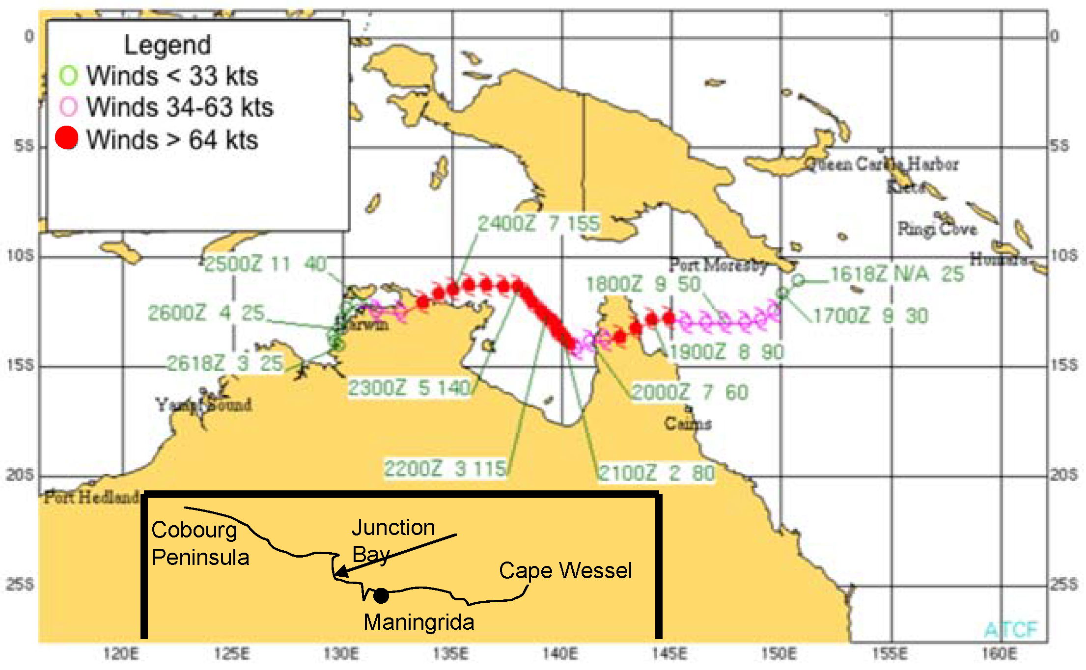
Figure 1.
Track of Cyclone Monica (courtesy JTWC). Inset at bottom of map (added by author) provides a simplified view of the Northern Territory, Australia area where Cyclone Monica made landfall (track show as arrow).
Figure 1.
Track of Cyclone Monica (courtesy JTWC). Inset at bottom of map (added by author) provides a simplified view of the Northern Territory, Australia area where Cyclone Monica made landfall (track show as arrow).

2. Cyclone Monica Overview
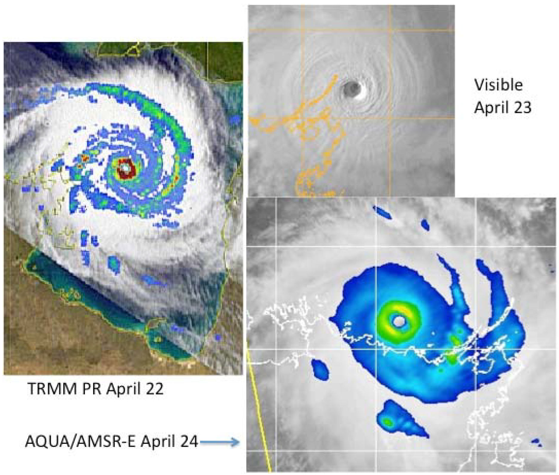
Cyclone Monica’s track is shown in Figure 1. It began as a tropical depression on 16 April 2006, in association with an equatorial Rossby wave [3]. From its formation area to the east of Papua New Guinea, it drifted southwest into the Coral Sea and intensified [4]; it was christened Cyclone Monica at 0000 UTC on 17 April. Upon reaching tropical storm strength, it took a more westward track and reached hurricane force prior to making its first landfall on the Queensland Australia coast on the afternoon of 19 April. It weakened as it crossed the Cape York Peninsula into the Gulf of Carpentaria. Once over water again it began to intensify rapidly as it moved northwestward. On 23 April it took a more westward track along the northern coast of the Northern Territory of Australia. It paralleled the coast and then turned southwest, making its second landfall around 1000 UTC on 24 April as an intense tropical cyclone. The location of landfall was in an unpopulated region at Junction Bay, over 40 km to the west of the town of Maningrida, as shown on the inset in Figure 1, based on the BOM track data [5]. Just prior to landfall, it actually came within about 35 km of Maningrida. Images of Cyclone Monica from spaceborne radar, visible, and passive microwave are shown in Figure 2 for the 22nd, 23rd, and 24th of April. An inspection of these images shows Monica to have been a very symmetric storm with a well-defined eye.
Figure 2.
Selected imagery of Cyclone Monica. (a) TRMM Precipitation Radar image at 1608 UTC on 22 April 2006. Maximum rain rate (dark red) exceeds 50 mm/h. (b) Visible imagery at 0900 UTC on 23 April 2006. (c) 85 GHz PCT image of Monica from NASA Aqua/AMSR-E at 0430 UTC on 24 April, overlaid on visible imagery. Yellow in eyewall is ~160 K. Courtesy US Navy/NRL-Monterey.

3. In situ Measurements and Damage Assessment
As noted in the introduction, there were no in situ measurements of Monica’s eyewall or eye. However, the center of Monica did pass near Cape Wessel, Australia on the 23rd. Prior to serious damage to the weather station there, a minimum pressure of 970 hPa was reported [6]. Based on radar imagery from Gove, Australia and BOM track data, the Cape Wessel measurement was taken somewhat outside the eyewall (40–50 km from the center of the eye). Monica was a small storm; the radar radius of maximum convection in the eyewall was about 20 km, assumed to be roughly the radius of maximum winds. Indeed, BOM estimated the radius of maximum winds at 19 km at this time [6]. Extrapolation of the pressure observation to MSLP could be done using Holland’s model [7]. The model pressure profile versus radius r is:
where penv is the environmental pressure (1005 hPa), pc is the MSLP, Rw is the radius of maximum wind speed, and B is a parameter that depends on storm size and structure. For various choices of B, r, and Rw, (1) can yield pressures from about 920 hPa down to values well below 900 hPa. Unfortunately, although the distance from the center to the observation is only 40–50 km, this distance is still rather large compared to storm size, making application of an exponential profile sensitive to errors in the input parameters. Other pressure observations (e.g., 986 hPa at Maningrida) were also well outside the eyewall. Courtney and Knaff [8] did extrapolate surface measurements to an MSLP of 920 hPa, but their method isn’t detailed.
p(r) = penv + (penv − pc)exp(−(Rw/r)B)
Damage reports from Maningrida, while significant, indicate that the sustained winds there were much less than the estimated maximum winds in the eyewall. A peak gust of 41 m/s was reported at Maningrida. Since the center of the eye came within about 35 km of Maningrida, the relatively sharp decrease in winds between the center and Maningrida suggests that Monica was still a compact storm at landfall. BOM estimated a radius of maximum winds at 22 m [6]. The compact size is further confirmed by the vegetation damage swath, reported as approximately 50 km [10]. Pictures on the BOM website of the vegetation in the landfall area show nearly complete defoliation and felled trees. Cook and Goyens [9] also note that the 50 km swath of destruction extended inland 130 km. As pointed out in [10], the damage appears similar to that seen in tornadoes; the trees were felled toward the ocean by the winds. BOM also reported evidence of a 5–6 m storm surge [6]. Heavy rainfall (up to 190 mm) was also reported as Monica moved inland on the 24th [6,11].
4. Intensity Estimates Based on the Dvorak Technique
Intensity estimates were provided by BOM, the Joint Typhoon Warning Center (JTWC), and the University of Wisconsin Cooperative Institute for Meteorological Satellite Studies (CIMSS). These estimates are based on the Dvorak technique [12,13] and are summarized in Table 1; estimates have been interpolated to the standard UTC observation times. BOM initially placed Monica’s peak intensity at 905 hPa [11]. The BOM final track summary, however, revised this upward to 916 hPa (with 79 m/s winds, one-minute average); this estimated intensity was reached at 0600 UTC on 23 April, staying nearly constant until landfall on the following day [5]. JTWC gave a peak intensity MSLP estimate of 879 hPa and 80 m/s [14]; the JTWC estimated peak intensity was reached around 1800 UTC on the 23rd and maintained until 0000 UTC on the 24th, followed by very slight weakening prior to landfall. The initial CIMSS estimate placed Monica’s MSLP at 869 hPa, which is just below the 870 hPa record measured by aircraft in Typhoon Tip in 1979 [1]. The CIMSS estimate is based on application of the automated Advanced Dvorak Technique (ADT), described by Olander and Velden [15]. The timing for this intensity estimate roughly coincides with the JTWC estimate. Application of updated ADT software still yields an MSLP of 870 hPa; however, this estimate uses the same pressure/wind relationship as the previous estimate. CIMSS also produced an estimate using a modified Knaff-Zehr relation, described in [8] for use in the Australia region. This yields a maximum wind of 81 m/s and an MSLP of 906 hPa, lasting from 0400 to 2000 UTC on the 23rd [16]. The higher MSLP is due to Monica’s low latitude and small size. In [8] the MSLP for a storm with 75 m/s (1-minute) winds is increased by 5 hPa, relative to the MSLP at larger latitude (25 versus 12 degrees) and larger size (radius gale force winds 110 versus 270 km). Since Monica was much smaller than even the smaller storm size in [8], a larger increase in MSLP would be expected. The estimated MSLP based on [8] with a 1005 hPa environmental pressure and very small size should be near 900 hPa, as in the CIMSS updated estimate.
A manual Dvorak analysis, such as used by Hoarau et al. on Typhoons Tip, Gay, or Angela [17], was also applied by Hoarau [18] to Monica, resulting in a maximum wind speed of 82 m/s and MSLP of 890 hPa. He also noted, however, that storms with intense pressure gradients could produce winds near 80 m/s even with MSLP slightly above 900 hPa. The four Dvorak-based peak intensity estimates are listed in Table 2. The wind speeds range from 79 to 82 m/s and are relatively close to each other. Since the wind speed is the primary Dvorak product, the greater variability in MSLP is likely due to the wind/pressure relations used to estimate MSLP from the maximum wind speed [8].
As a comparison, Cyclone Orson of 1989 was one of the few storms near Australia to have had an in situ measurement of its MSLP near peak intensity as it passed over an oil platform northwest of Australia. Orson’s measured MSLP was 905 hPa; its presentation on enhanced infrared is similar to Monica’s but was rated slightly lower on the Dvorak scale [19]. This could argue for an MSLP of less than 905 hPa for Monica, but Monica may have been somewhat smaller in size.

Table 1.
Intensity estimates versus time for BOM, JTWC, and CIMSS. BOM 10-minute average maximum wind speeds were converted to 1-minute average using a multiplying factor of 1.14. Estimates have been interpolated to standard times for comparison.
| Time | BOM MSLP/Max Wind (hPa, m/s) | JTWC Max Wind (m/s), no MSLP | CIMSS ADT MSLP/Max Wind (hPa, m/s) |
|---|---|---|---|
| 22 Apr 2006 00:00 | 947/59 | 59 | 936/55 |
| 22 Apr 2006 06:00 | 935/65 | 64 | 930/65 |
| 22 Apr 2006 12:00 | 928/73 | 64 | 930/71 |
| 22 Apr 2006 18:00 | 928/73 | 67 | 927/71 |
| 23 Apr 2006 00:00 | 929/73 | 72 | 912/76 |
| 23 Apr 2006 06:00 | 916/79 | 77 | 906/81 |
| 23 Apr 2006 12:00 | 919/79 | 80 | 906/81 |
| 23 Apr 2006 18:00 | 917/79 | 80 | 906/81 |
| 24 Apr 2006 00:00 | 919/79 | 80 | 906/81 |
| 24 Apr 2006 06:00 | 917/79 | 80 | 906/80 |
| 24 Apr 2006 12:00 | 954/53 | 59 | 909/60 |
| Method | Maximum Wind Speed (m/s) (1-minute averaging time) | MSLP (hPa) |
|---|---|---|
| Dvorak–BOM | 79 | 916 |
| Dvorak–JTWC | 80 | 879 |
| Advanced Dvorak–CIMSS | 81 | 906 |
| Manual Dvorak–Hoarau | 82 | 890 |
5. Satellite Remote Sensing of Intensity
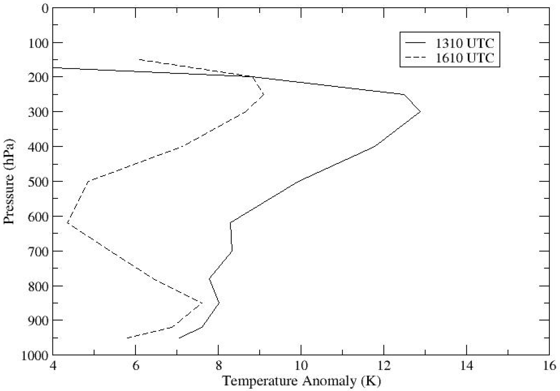
This section describes analyses of other satellite datasets that provide additional clues as to the peak intensity of Monica. The data used generally fall into the class of either sounding or imaging. In the case of infrared sounding, multiple spectral channels are inverted for temperature and humidity profiles [20]. If such profiles can be obtained in the eye, it is possible to directly integrate the hydrostatic equation to get surface pressure [21,22]. Figure 3 shows the eye temperature anomaly profiles from the Moderate Resolution Imaging Spectrometer (MODIS) for the only two passes over Monica with usable data in the eye; other passes from late on the 22nd to early on the 24th had too much cloud cover for profile retrieval. The temperature anomaly is the difference between the temperature profile retrieved within the eye and the environmental temperature profile outside the storm. The maximum anomaly is 13 K in the 1310 UTC pass. To estimate the surface pressure we begin with the hydrostatic equation:
![Atmosphere 01 00015 i001]() where R is the gas constant, g is gravitational acceleration, and T(p) is the retrieved temperature at pressure level p. To include moisture effects, we use the virtual temperature, rather than the ordinary temperature. We assume that the height of the 100 hPa pressure surface is the same both inside and outside the storm. This implies that the integral of this equation from surface to 100 hPa should be the same both inside and outside.
where R is the gas constant, g is gravitational acceleration, and T(p) is the retrieved temperature at pressure level p. To include moisture effects, we use the virtual temperature, rather than the ordinary temperature. We assume that the height of the 100 hPa pressure surface is the same both inside and outside the storm. This implies that the integral of this equation from surface to 100 hPa should be the same both inside and outside.

Figure 3.
Temperature anomaly profiles from MODIS data for Terra pass at 1310 UTC and Aqua pass at 1610 UTC on 23 April 2006.
Figure 3.
Temperature anomaly profiles from MODIS data for Terra pass at 1310 UTC and Aqua pass at 1610 UTC on 23 April 2006.

This leads to the following equation that we solve for the eye pressure pc:
![Atmosphere 01 00015 i002]() where ps is the environmental surface pressure, and the pressure at the top of the storm or in the environment pt is 100 hPa. We fit 5th order polynomials to the retrieved temperature profiles to carry out the integrations in (3). This technique gives 955 hPa at 1310 and 965 hPa at 1610 at the location of the MODIS pixels, both of which are away from the eye center, adjacent to the eyewall. As noted by Willoughby [23] an additional 20% or so of the total pressure drop occurs between the eyewall and eye center, so it is reasonable to adjust the MODIS retrievals downward by 10 hPa to better estimate the MSLP at each time. This yields 945 hPa at 1310 and 955 hPa at 1610, still considerably higher than expected. The MODIS profile data have very good spatial resolution (5 km) but rather poor spectral and, hence, vertical resolution [24]. Hence, it is possible that the vertical resolution was too coarse to see the true temperature anomaly over the eye.
where ps is the environmental surface pressure, and the pressure at the top of the storm or in the environment pt is 100 hPa. We fit 5th order polynomials to the retrieved temperature profiles to carry out the integrations in (3). This technique gives 955 hPa at 1310 and 965 hPa at 1610 at the location of the MODIS pixels, both of which are away from the eye center, adjacent to the eyewall. As noted by Willoughby [23] an additional 20% or so of the total pressure drop occurs between the eyewall and eye center, so it is reasonable to adjust the MODIS retrievals downward by 10 hPa to better estimate the MSLP at each time. This yields 945 hPa at 1310 and 955 hPa at 1610, still considerably higher than expected. The MODIS profile data have very good spatial resolution (5 km) but rather poor spectral and, hence, vertical resolution [24]. Hence, it is possible that the vertical resolution was too coarse to see the true temperature anomaly over the eye.

We were also able to obtain an Atmospheric Infrared Sounder (AIRS) sounding close to the eye center at 1610 at 15 km horizontal resolution via special processing at CIMSS [25]; the standard horizontal resolution is 45 km, which is too coarse to resolve the tropical cyclone eye in many cases. AIRS operates only on the Aqua platform, so AIRS data at 1310 are not available. Although the horizontal spatial resolution is coarser than MODIS, the vertical resolution is much better due to the many AIRS channels (Seemann et al. [24]). The maximum temperature anomaly in the AIRS retrieval is 11 K, about 2 K larger than found from the MODIS data for the same time. The retrieved MSLP using the 1610 GMT AIRS data is 954 hPa, very close to the corrected MODIS measurement. The 15-km footprint of AIRS is still rather coarse relative to the 35 km eye diameter (based on microwave imagery), so some downward correction in the AIRS estimate is probably also appropriate. While the retrieved MSLP (even with some downward adjustment) is indicative of a major tropical cyclone, it is well above the values in Table 1 and Table 2 and raises questions about the retrieval methodology. There are at least three possible explanations: (1) Monica’s actual MSLP was higher than originally estimated, at least at the time of the MODIS observations, (2) the satellite temperature profiles from both AIRS and MODIS are flawed, or (3) the method of finding MSLP based on (3) is incorrect.
To assess the third explanation, a simpler version of the retrieval method was developed by parameterizing the temperature anomaly profile. This allows use of temperature anomalies observed by aircraft reconnaissance to estimate MSLP and compare with the MSLP directly measured by dropsondes. To do this, we rewrite (3) by breaking the integral on the right side into two parts:
![Atmosphere 01 00015 i003]()

Both of the integrals from pt to pc in (4) can be combined into a single integral of the temperature anomaly. This integral is then equal to the integral of the environmental temperature profile from the central pressure down to the environmental surface pressure:
![Atmosphere 01 00015 i004]()

The right side of (5) can be computed using a mean environmental sounding, in this case that of Jordan [26]. For the left side of (5), the temperature anomaly from past storms [27] was used to get an approximate form. It tends to increase rapidly from 100 to 200 hPa and then slowly drop to the 600 hPa level, followed by a drop to near zero at the surface. It is approximated with a 5th order polynomial. The central pressure pc is then chosen to satisfy (5). Table 3 shows the results of using this technique for various historic storms. Information for these storms is provided in [21] and [28,29,30,31,32]; the MSLP estimate for Zeb would likely have been higher for a smaller storm with similar features. The MSLP estimated using (5) is in reasonable agreement with the observed MSLP, given the uncertainties in the measurements and variability of storm size and location. The storms in Table 3 varied from large typhoons to very small hurricanes. Inez, for example, had a radius of maximum wind of less than 20 km [29] and was thus similar in size to Monica. It seems that the estimated MSLP of 944 hPa is consistent with the 13 K temperature anomaly. An MSLP of less than 900 hPa should correspond to an anomaly of at least 20 K; indeed the mean typhoon of Frank [27] has an upper level temperature anomaly maximum of 15 K. Hence, the conversion between eye temperature and MSLP seems reasonable and so is eliminated as a significant source of error.
Table 3.
MSLP estimated from simplified model using temperature anomaly as input. Temperature anomaly and observed MSLP are based on aircraft measurements unless otherwise noted.
| Tropical Cyclone | Max Temperature anomaly (K) | Estimated MSLP using (5) (hPa) | Observed MSLP (hPa) |
|---|---|---|---|
| Monica (4/23, 1310 UTC) | 13 | 945 | - |
| Monica (4/23, 1610 UTC) | 11 | 956 | - |
| Erin (2001) | 11 | 956 | 968 |
| Bonnie (1998) | 14 (AMSU) | 941 | 954 |
| Oliver (1993) | 10 | 959 | 950 |
| Georges (1998) | 14 (AMSU) | 941 | 939 |
| Inez (1966) | 16 | 931 | 927 |
| Floyd (1999) | 18 (AMSU) | 923 | 924 |
| Mitch (1998) | 19 (AMSU) | 918 | 917 |
| Zeb (1998) | 20 (AMSU) | 913 | 900 (Dvorak) |
| Marge (1951) | 20 @ 500 hPa 24@ 200 hPa (est) | 896 | 895 |
Could the temperature retrievals for both AIRS and MODIS underestimate the temperature anomaly? Resolution and sampling can have an impact as noted above. Apart from these error sources, it seems unlikely that the profiles retrieved from both sensors using different algorithms would seriously underestimate the anomaly. Another potential source of error in both retrievals is the use of global numerical forecast model surface pressure as input. Due to poor resolution, the surface pressures are usually close to environmental (too high by up to 100 hPa or so). Experiments with a radiative transfer code, however, suggest that the impact on the retrieved profiles is likely small. The largest reasonable temperature anomaly would use 13 K at 1310 and increase it by 3–4 K due to resolution and sampling errors (based on simulations with Gaussian-shaped anomaly fields and sensor responses). A 16–17 K temperature anomaly corresponds to an MSLP of about 930 hPa at 1310 UTC.
Based on evaluation of the second and third explanations for the higher values of MSLP, the first explanation, that Monica actually had a higher MSLP at the times of MODIS and AIRS sampling, seems likely. Since, the number of MODIS and AIRS soundings is very limited due to cloud cover in the eye, it is possible that Monica had reached a greater intensity earlier and had weakened somewhat by the time of the soundings. Indeed, the MODIS sounding at 1310 UTC on the 23rd gives a larger temperature anomaly than a pass three hours later, indicative of weakening. This is examined with additional data in the following.
Microwave sounders such as the Advanced Microwave Sounding Unit (AMSU) [30] and the Special Sensor Microwave Imager Sounder (SSMIS) [33] provide an alternative to AIRS and MODIS. Temperature and humidity profiles can be retrieved using algorithms similar to those for infrared sounding (see, for example, Staelin [34]), with the advantage of less impact due to clouds. However, microwave sensors have relatively coarse resolutions (50 km for AMSU and 40 km for SSMIS), so the observed brightness temperature must be deconvolved [35] prior to a physically-based retrieval or statistically-based retrieval [22,36]. CIMSS routinely generates an MSLP estimate based on a statistical regression relating AMSU data to MSLP. Their AMSU product for Monica reports a minimum MSLP of 903 hPa and maximum wind of 85 m/s [16]. Direct examination of the AMSU data shows that the channel 8 (55.5 GHz) anomaly peaks at 5 K on April 23. The anomaly in SSMIS channel 5 (55.5 GHz) data is also 5 K; the anomaly in channel 4 (54.4 Hz) is about 0.5 K lower. For comparison, the channel 4 SSMIS maximum anomaly for Katrina is 7.5 K, with MSLP 902 hPa [33], but Katrina was a larger storm, so its anomaly should have been better resolved. Using the CIMSS regression between the channel 8 anomaly and MSLP [37] gives an MSLP of around 920 hPa, but with large error bars. The CIMSS AMSU product estimate of 903 hPa depends on the raw maximum anomaly, deconvolution of the brightness temperature estimates, and corrections for attenuation, scattering, and sampling error. These steps are particularly important for storms as small as Monica. CIMSS also produces a satellite consensus (SATCON) product that makes use of both ADT and AMSU estimates; the maximum intensity in their SATCON product is 80 m/s and 904 hPa, early on the 23rd. The intensity decreases to 68 m/s and 928 hPa near landfall [16], so Monica would have been weakening at the time of the soundings from AIRS and MODIS. It is interesting that the weakening trend in the SATCON estimates is based on microwave data. While the ADT MSLP rises only slightly, to 909 hPa (see Table 1), the AMSU MSLP rises to 930 hPa at landfall.
An alternative to sounders is microwave and infrared imagers that respond to precipitation and clouds. However, imagers provide no vertical information, so intensity must be estimated from either the absolute brightness temperature or from relative variation between pixels (i.e., texture). Several studies have related the microwave brightness temperature to storm intensity. Cecil and Zipser [38] find that the inner core average 85-GHz polarization corrected temperature (PCT) is correlated with the intensity. Hoshino and Nakazawa [39] find that the minimum 10-GHz horizontally polarized brightness temperature within 0.5° distance of the center has the highest correlation with intensity. They also find that the averaged 10-GHz horizontally polarized brightness temperature within 1° of the center is correlated with intensity.
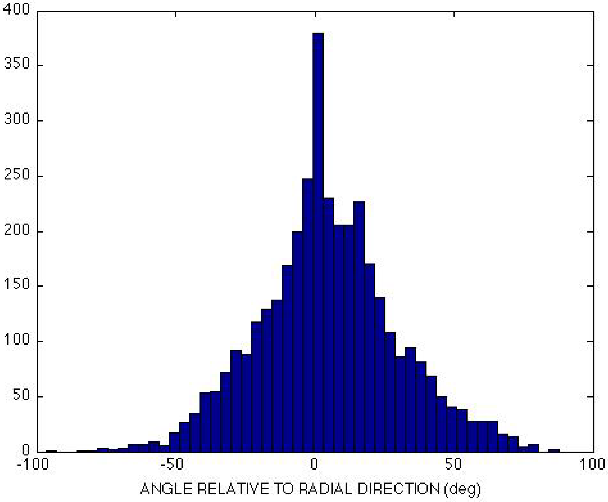
Figure 4.
Histogram of IR brightness temperature gradient vectors relative to radial direction for Cyclone Monica 1610 UTC MODIS data. Y-axis is relative count. The variance computed from this histogram is 508 degrees-squared.
Figure 4.
Histogram of IR brightness temperature gradient vectors relative to radial direction for Cyclone Monica 1610 UTC MODIS data. Y-axis is relative count. The variance computed from this histogram is 508 degrees-squared.

Taking a different approach, Pineros et al. [40] estimated intensity by calculating the statistics of gradient vectors of geostationary IR data. Since the gradient vector always points in the direction of maximum change, a circularly symmetric image would have all gradient vectors pointing at the center. As the distribution deviates from perfectly symmetric, the distribution of the angular direction of the vectors broadens. Since the more intense storms are more symmetric, their brightness temperature gradient vectors all point toward the storm center, with small standard deviation. Weaker, asymmetric storms tend to have a much broader spread in the gradient vector angle. Figure 4 shows a histogram of the gradient vectors obtained from a MODIS 10.7 micrometer image of Monica.
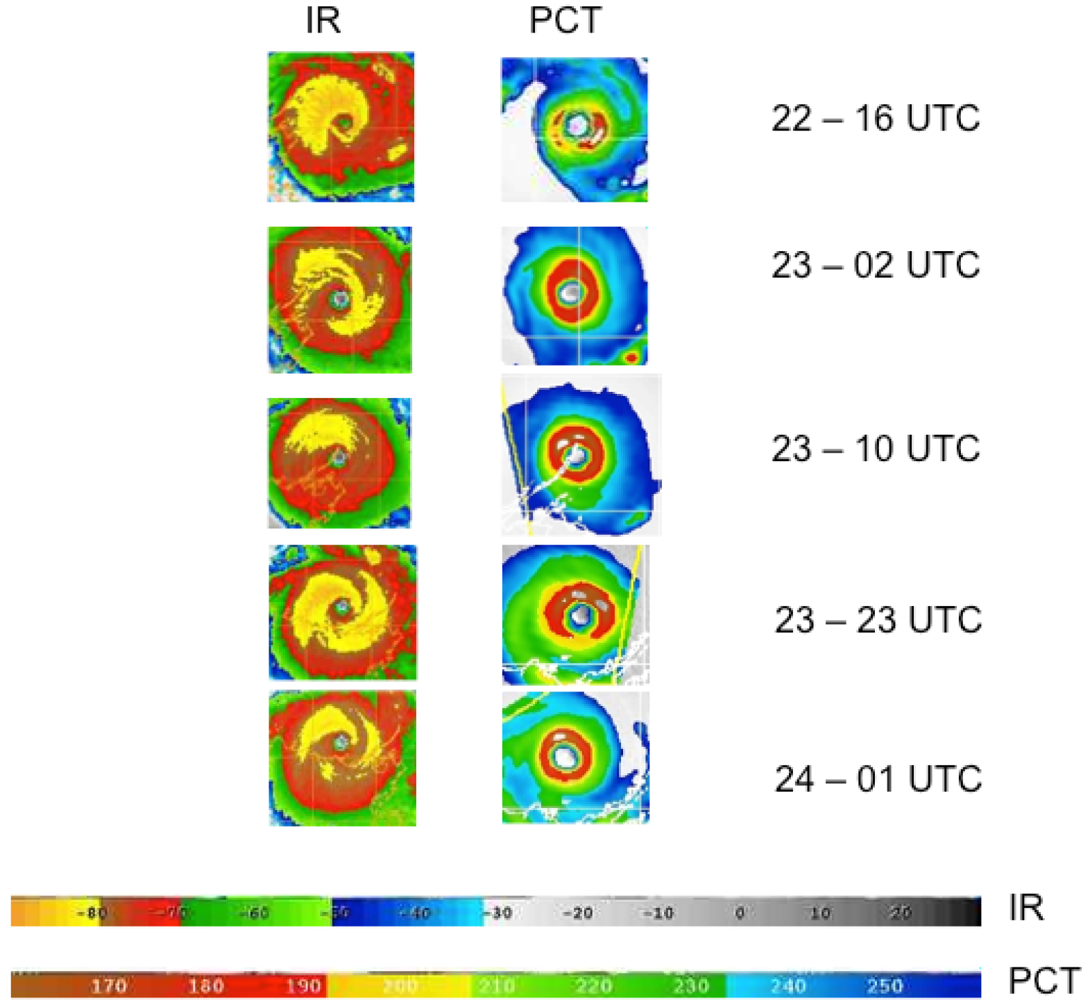
Figure 5.
Sequence of geostationary infrared and 85 GHz PCT images for Monica. Courtesy US Navy/NRL-Monterey. PCT images are from TRMM TMI and DMSP SSMIS.
Figure 5.
Sequence of geostationary infrared and 85 GHz PCT images for Monica. Courtesy US Navy/NRL-Monterey. PCT images are from TRMM TMI and DMSP SSMIS.

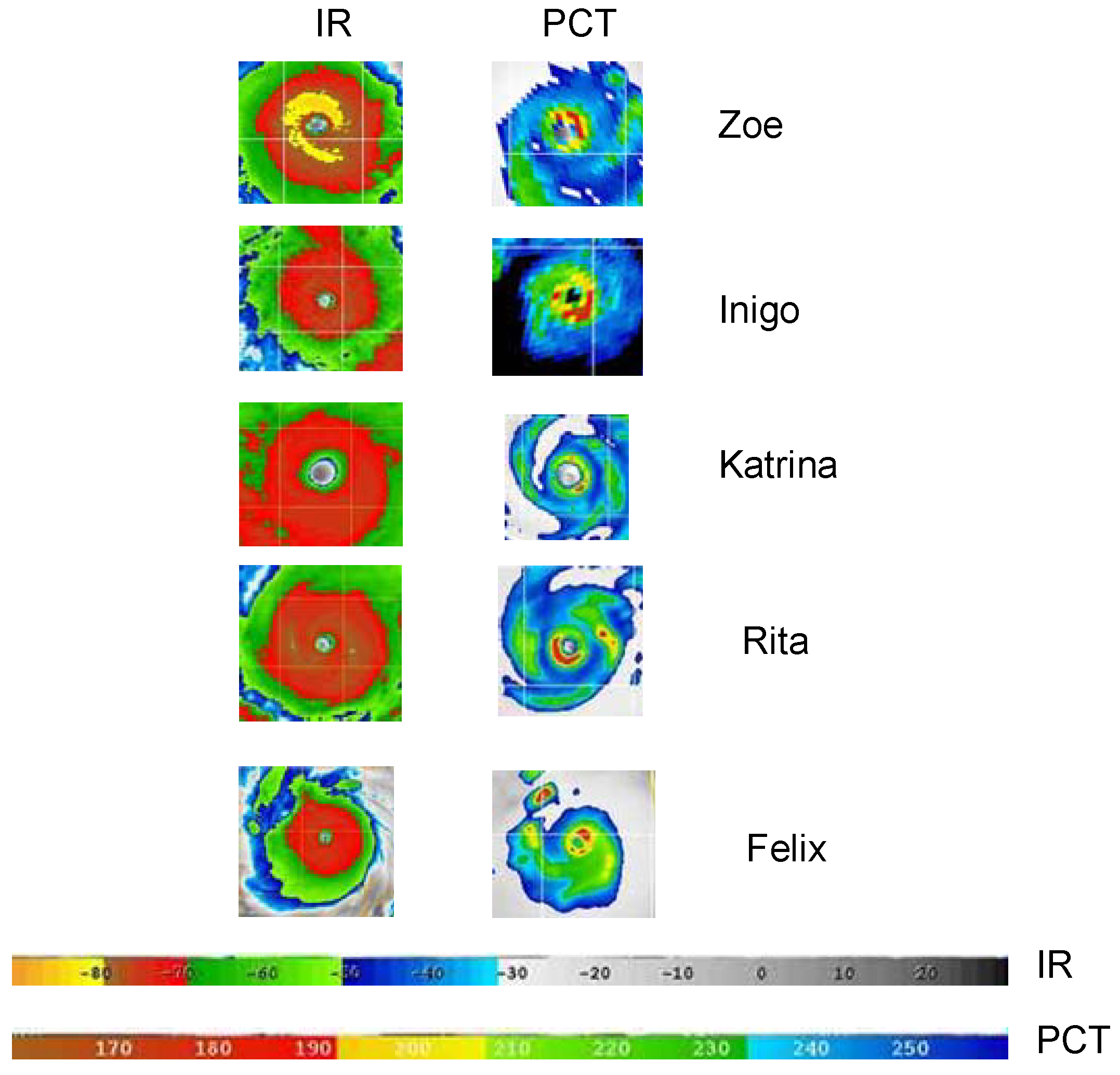
To assess Monica’s intensity from imagery, comparison of image characteristics of Monica and several other intense storms is performed. The image characteristics are derived in exactly the same way for each storm to avoid the need to “calibrate” the calculations here with those presented in the references for the image-based techniques discussed above. Figure 5 shows the time sequence of microwave and infrared imagery throughout the period of peak intensity from late on the 22nd to early on the 24th. Maximum intensity appears to be early on the 23rd; by 2300 UTC on the 23rd, the eyewall has lost its symmetry. By 0100 UTC on the 24th eyewall convection has regained symmetry but is diminished in intensity as seen in the microwave image (the average PCT is warmer). Figure 6 shows the microwave and infrared imagery for several other storms near peak intensity. Cyclones Zoe in 2002 [19] and Inigo in 2003 were both intense Southern Hemisphere storms; information on them is based on information from BOM, derived from satellite imagery, and so is subject to the same uncertainties as values for Monica. Katrina and Rita in 2005, and Felix in 2007 were Atlantic hurricanes; their MSLP and maximum wind speeds were measured by aircraft. Katrina was larger than Monica, while Rita and Felix were relatively compact storms just after reaching their maximum intensities. The eye diameter of Felix decreased to a small size of about 20 km in diameter, based on information from the National Hurricane Center. Table 4 compares the characteristics of these storms. The angular variances for all storms were computed from MODIS 10.7-micrometer images with averaging to 5 km resolution. Not shown are additional calculations for Katrina after it had begun to weaken (angular variance 886) and Rita just prior to reaching hurricane intensity (angular variance 1089). A comparison of the storm parameters in Table 4 and visual comparison of the imagery in Figure 5 and Figure 6 confirm that Monica’s characteristics compare quite well with other intense tropical cyclones, although the variation in size and location make inference of Monica’s absolute intensity from this comparison somewhat uncertain. At the least, this comparison does not justify a substantial reduction in the maximum wind speed from the Dvorak estimates, so a minimum wind speed of at least 75 m/s is chosen. Table 5 summarizes peak intensity estimates for the various sensors.
Figure 6.
Geostationary infrared and 85 GHz PCT images near peak intensity for five other tropical cyclones: Cyclone Zoe (2002), Cyclone Inigo (2003), Hurricane Katrina (2005), Hurricane Rita (2005), and Hurricane Felix (2007). Courtesy US Navy/NRL-Monterey.
Figure 6.
Geostationary infrared and 85 GHz PCT images near peak intensity for five other tropical cyclones: Cyclone Zoe (2002), Cyclone Inigo (2003), Hurricane Katrina (2005), Hurricane Rita (2005), and Hurricane Felix (2007). Courtesy US Navy/NRL-Monterey.

Table 4.
Comparison of satellite observed parameters for Monica and several other intense cyclones at peak intensity. Maximum surface winds are 1-minute average.
| Monica | Zoe | Inigo | Katrina | Rita | Felix | |
| MSLP (hPa) | 916 | 890 | 900 | 902 | 895 | 929 |
| Maximum wind (m/s) | 79 | 80 | 76 | 77 | 79 | 77 |
| IR Angular Var (deg2) | 508 | 583 | 665 | 582 | 461 | 500 |
| IR Tb Avg (C) | −83 | −83 | −78 | −75 | −79 | −73 |
| PCT Avg (K) | 195 | 205 | 200 | 215 | 200 | 200 |
| 10-GHz H Tb Min (K) | 147 | 191 | 170 | 185 | 193 | 145 |
| 10-GHz H Tb Avg (K) | 170 | 204 | 164 | 198 | 198 | 163 |
| Platform/ Mission | Sensor | Method | Intensity (MSLP or maximum wind speed) |
|---|---|---|---|
| Aqua/Terra | MODIS | Level 2 retrieved profiles in eye with hydrostatic equation | 945 hPa |
| Aqua | AIRS | CIMSS single FOV profile in eye w/ hydrostatic equation | 954 hPa |
| Aqua/Terra | MODIS/AIRS | Correction for resolution/sampling | 930 hPa |
| NOAA - ## | AMSU-A | CIMSS estimate from brightness temperature anomaly [16] | 903 hPa, 85 m/s |
| NOAA – ## | AMSU-A | CIMSS SATCON combined ADT and microwave estimate [16] | 904 hPa, 80 m/s |
| DMSP | SSMIS | 55.5 GHz brightness temperature anomaly of 5 K with CIMSS statistical relation in [37] | 920 hPa |
| Aqua TRMM DMSP | AMSR-E TMI SSMI/SSMIS | 85-GHz PCT average around eyewall; 10-GHz min and mean | ≥75 m/s |
| Terra | MODIS | Gradient angular variance | ≥75 m/s |
6. Maximum Potential Intensity
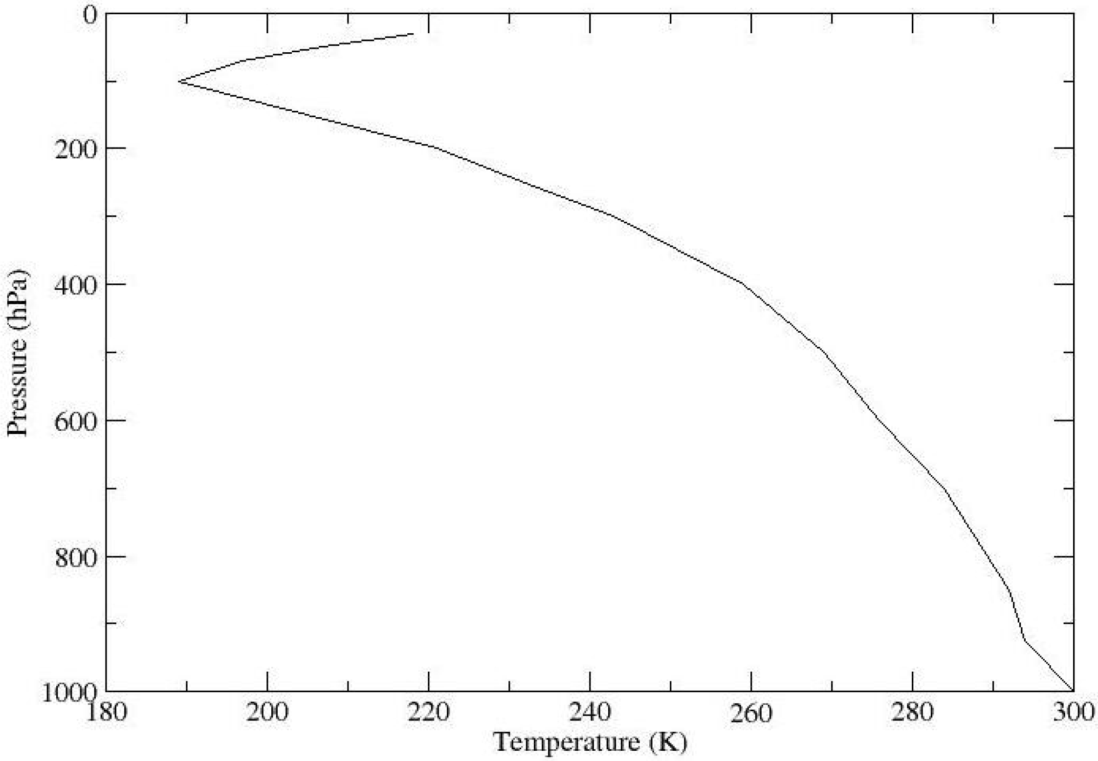
Beyond satellite measurements of the storm itself, also it is possible to utilize satellite estimates of Monica’s environment, e.g., temperature and moisture profile and sea surface temperature (SST) as input to various models that provide intensity estimates. Figure 7 shows an AIRS temperature sounding of the environment prior to Monica’s passage; the SST reported by AIRS was 302−303 K, which is in good agreement with SST maps provided by BOM. This information allows an estimate of the maximum potential intensity (MPI) using the method described by Emanuel [41,42]. Using an SST of 302.5 K, Emanuel’s model yields an MPI of 82 m/s and 873 hPa.
Figure 7.
Environmental sounding from NASA Aqua/AIRS instrument, used in calculation of Emanuel’s MPI and initialization of axisymmetric models.
Figure 7.
Environmental sounding from NASA Aqua/AIRS instrument, used in calculation of Emanuel’s MPI and initialization of axisymmetric models.

At the next level of complexity are axisymmetric models [43,44]. The three-layer model of Emanuel reaches an initial equilibrium at 80 m/s and 874 hPa. The Rotunno and Emanuel model with 17 layers in the vertical reaches a minimum MSLP of 856 hPa with winds of 108 m/s. Based on results from an improved axisymmetric model, the intensity reached by the Rotunno/Emanuel model should be reduced by about 10% [45]. The adjusted Rotunno/Emanuel model results are 870 hPa and 97 m/s. While axisymmetric models cannot accurately simulate a particular tropical cyclone, they do provide an estimate of the MPI in a particular environment [45].
These results would imply that Monica was near its MPI, if the MSLP were, indeed, below 880 hPa. Wind shear over the storm’s core was low (less than 5 m/s); maximum shear occurred to the east of the storm reaching close to 10 m/s on the 24th. While the low shear could argue for an intensity near MPI, the ocean heat content in this area appears to be lower than might be expected from SST. Climatological maps of the 26-degree C isotherm depth indicate a maximum of about 70 m for this area in late summer, shallower than, for example the Caribbean Sea. In fact, the physical depth of the ocean over which Monica reached its peak is 70 m or less. The shallow ocean and the proximity to land may have kept Monica from reaching its MPI. Furthermore, the MPI calculations do not explicitly account for storm size and could overestimate the pressure drops for small storms.
7. Modeling with WRF
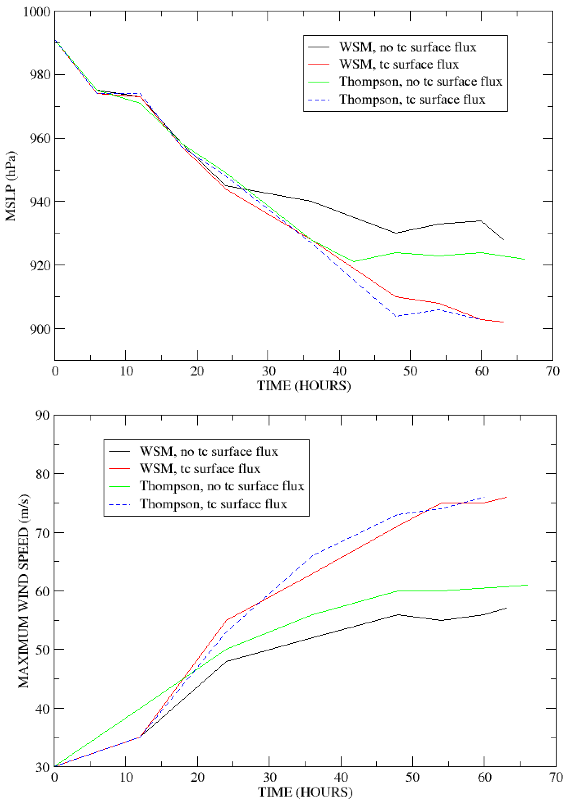
The WRF model has been previously used to simulate historical tropical cyclones (e.g., [46]), and similar methodology is used here. The National Centers for Environmental Prediction (NCEP) analysis provides an initial condition to simulate Monica. Because the NCEP analysis uses too large a grid spacing to properly resolve the cyclone, a bogus vortex was generated using the bogussing facility now available in WRF 3.1. Without the bogus, the storm takes an unrealistically long time to spin up. We performed four runs using a bogus vortex; the difference between the runs is the selection of microphysics scheme (either WSM/6 or Thompson/8) and surface fluxes (either normal or enhanced for tropical cyclones).
The enhanced tropical cyclone flux option is new in WRF 3. Further information on WRF options is available in the user’s guide [47]. All runs used a nested domain with grid spacings of 9, 3, and 1 km with cumulus parameterization turned on for the 9 km grid only; explicit convection is used at the two smaller spacings. All runs also used the Yonsei University boundary layer parameterization. Although the SST update option is set to update the SST with NCEP data during the simulations, cooling of the surface due to the storm is not captured in the NCEP data and thus not taken into account by these WRF runs.
The runs all start with the same bogus vortex near hurricane strength placed on Monica’s track in Figure 1 near 142° E longitude, just off the west coast of the Cape York Peninsula. The runs initially follow Monica’s actual track; they all head northwest and then turn west. However, none make the southwest turn toward the Australian coast; they continue west, remaining at sea. Figure 8 shows the maximum wind and MSLP as a function of time; each simulation was considered to end when the storm center moved west of 133° E longitude, which is the westernmost longitude of Monica’s track (reached at landfall). The run with the WSM microphysics and without the tropical cyclone surface fluxes generates a strong tropical cyclone with winds near 57 m/s and MSLP of 928 hPa. The run using the same flux option but Thompson microphysics becomes a stronger storm with MSLP of 923 hPa and 60 m/s winds. When the WRF tropical cyclone surface flux option is used, more intense cyclones result: 902 hPa for WSM and 903 hPa for Thompson microphysics. The maximum wind speed is 76 m/s for both cases, which is closer to the various satellite estimates. While various choices of microphysics parameterizations have been used for hurricane simulations, the Thompson microphysics may be more realistic. Fierro et al. [46] point out that the WSM scheme produces too much graupel relative to graupel observations in hurricanes. Indeed, the simulations with WSM in this work did produce more graupel in the eyewall than the Thompson scheme. The WRF intensities are reasonably consistent with the estimates in Table 5, although somewhat lower than the Dvorak estimates, especially without enhanced surface flux.
To determine how well the intensity of Monica is modeled by the various WRF runs, we could compare satellite observations with the corresponding WRF model parameters. Ideally, we would run the WRF model output through satellite sensor models and then compare the model-generated satellite data with the actual data. While this is beyond the scope of this paper, it could be a useful way to test WRF simulations of specific storms. Here, we settle for comparing the size and temperature anomaly with satellite observations. As noted previously, the eye diameter of Monica as observed in microwave imagery is approximately 35 km. The eye diameter estimates based on the WRF model prediction of the eyewall rain water content are all within a few km of the observed value. The run with Thompson microphysics and enhanced fluxes had an eye shape slightly closer to the circular eye seen in microwave imagery of Monica.
Figure 8.
WRF simulations MSLP (upper) and maximum surface winds (lower) versus time.

WRF also outputs the potential temperature field, which can be used to estimate the temperature anomaly over the eye. When the enhanced surface fluxes are used, the maximum upper level temperature anomalies predicted by WRF are 23 K (WSM) and 20 K (Thompson). For the two runs without the enhanced fluxes, the temperature anomalies are around 13 K, lower than the maximum MODIS/AIRS estimate of 16–17 K. The 23 K anomaly, in contrast, seems too large. However, a 19 K anomaly at peak intensity followed by weakening is not too out of line with the MODIS/AIRS maximum. This, combined with a 33-km circular eye, make the Thompson with enhanced fluxes a slightly better fit to the observations than the other runs. However, due to uncertainties in tropical cyclone modeling, these results should be weighted relatively low in estimating Monica’s true intensity.
8. Summary and Conclusions
A range of peak intensity MSLP estimates were reported for Cyclone Monica of 2006, although peak wind speed estimates are closer together, near 80 m/s. Evidence from remote sensing and modeling confirms that it was an intense tropical cyclone. It was a very symmetric storm in visible, infrared and microwave imagery, so the Dvorak-based MSLP estimates below 880 hPa are not unreasonable. The calculated maximum potential intensity was also below 880 hPa. Arguing for a much higher MSLP, however, are the temperature anomalies estimated from MODIS and AIRS. Even with downward correction for resolution and other errors, it would be difficult to justify an MSLP below 930 hPa at 1310 UTC on the 23rd. In between these two extremes are estimates from microwave sounding and image data, comparison with a similar intense storm with in situ measurement of MSLP (Orson), and the extrapolation from surface measurements in [8]. WRF model runs also fall into this middle ground. All these data taken together argue that the peak intensity is slightly lower (less intense) than those estimated from the Dvorak technique alone (Table 2). Furthermore, Monica may have weakened more following its peak than was evident in the visible/IR imagery used for the Dvorak analyses.
The Dvorak peak intensity MSLP estimates are likely to be more uncertain than the maximum wind estimates due to the relationships used to derive them from the maximum wind speed. Specifically, the relation to convert wind speed to MSLP should be appropriate for the region north of Australia, particularly the low latitude and small storm size [8,48]. The best MSLP estimate is likely somewhere in the middle of the data summarized above; the lower bound of the range of possible MSLPs is chosen as 900 hPa, with 920 hPa as the upper bound. The upper bound is lower than the infrared sounding results in Table 5, since the soundings were probably made after Monica had started weakening. However, it seems unlikely that the MSLP could have risen by more than around 30 hPa on the 23rd between peak intensity and 1310 UTC, so we take 900 hPa as the minimum.
Unlike MSLP, the temperature anomaly doesn’t have a very direct relation to maximum wind speed, so the top end of the range of maximum wind speeds is chosen as the 82 m/s Dvorak estimate. An uncertainty range of 10 m/s seems reasonable, giving a lower limit of 72 m/s and more than covering the range of estimates in Table 5. Hurricane Felix, as shown in Table 4, demonstrates that a small storm can have winds in this range even with MSLP above the upper bound for Monica. At the time of landfall, roughly 24 hours after its probable peak intensity, Monica may have weakened by up to 10 m/s and 20 hPa, based on the retrieved temperature anomalies and the CIMSS AMSU product. Even so, it was still strong enough to produce a large storm surge and extensive vegetation damage.
Acknowledgements
The author would like to thank Mark DeMaria of NOAA/NESDIS for providing information on his method for estimation of intensity from satellite soundings and K. A. Emanuel of MIT for making his MPI and hurricane codes publicly available. Help from Simone Tanelli (of JPL) in setting up WRF and solving WRF run-time problems is greatly appreciated, as is the AIRS profile provided by Elisabeth Weisz and Jun Li of CIMSS. The author also thanks Karl Hoarau for providing the results of his manual Dvorak analysis of Cyclone Monica and additional comments on tropical cyclone intensity and Dvorak analysis. T. Olander, C. Velden, and D. Herndon of CIMSS generated new ADT, AMSU, and SATCON products for Monica. They also provided comments and suggestions on a draft of the manuscript, and D. Herndon pointed out the existence of the Cape Wessel observations. Anu Dudhia provided the RFM radiative transfer code. Finally, the author thanks one of the anonymous reviewers, who is clearly very familiar with this tropical cyclone and whose comments substantially improved the accuracy and clarity of this paper. The research described in this paper was carried out at the Jet Propulsion Laboratory, California Institute of Technology, under contract with the National Aeronautics and Space Administration.
References and Notes
- Dunnavan, G.M.; Diercks, J.W. An analysis of Super Typhoon Tip (October 1979). Mon. Wea. Rev. 1980, 108, 1915–1923. [Google Scholar] [CrossRef]
- Skamarock, W.C.; Klemp, J.B. A time-split nonhydrostatic atmospheric model for weather research and forecasting applications. J. Comp. Phys. 2008, 227, 3465–3485. [Google Scholar] [CrossRef]
- Callaghan, J.; Otto, P.; Ready, S.; Smith, T.; Waqaicelua, A. Operational Forecasting of Tropical Cyclone Formation. In Proceedings of the 6th WMO International Workshop on Tropical Cyclones; Jose, S., Rica, C., Eds.; November 21-30 2006; pp. 288–304. [Google Scholar]
- Courtney, J.B.; Santos, B.J. The South Pacific and Southeast Indian Ocean tropical cyclone season 2005-06. Aust. Met. Mag. 2008, 57, 53–64. [Google Scholar]
- BOM (Australian Bureau of Meteorology). Raw cyclone track data—2007 repair. Available online: ftp://ftp.bom.gov.au/anon2/home/ncc/cyclone/Newcyclonedatabase.zip/ (accessed on May 20, 2010).
- BOM (Australian Bureau of Meteorology). Severe Tropical Cyclone Monica. Available online: http://www.bom.gov.au/announcements/sevwx/nt/nttc20060417.shtml/ (accessed on January 9, 2010).
- Holland, G.J. An analytic model of the wind and pressure profiles in hurricanes. Mon. Wea. Rev. 1980, 108, 1212–1218. [Google Scholar] [CrossRef]
- Courtney, J.; Knaff, J.A. Adapting the Knaff and Zehr wind-pressure relationship for operational use in tropical cyclone warning centers. Aust. Met. Mag. 2009, 58, 167–179. [Google Scholar]
- Cook, G.D.; Goyens, C.M.A.C. The impact of wind on trees in Australian tropical savannas: lessons from Cyclone Monica. Austral Ecology 2008, 33, 462–470. [Google Scholar] [CrossRef]
- Kieper, M. Revisiting Cyclone Monica. 2007. Available online: http://www.wunderground.com/blog/MargieKieper/comment.html?entrynum=134&tstamp=200701/ (accessed on May 24,2010).
- BOM (Australia Bureau of Meteorology). Significant Weather—April 2006. Available online: http://www.bom.gov.au/inside/services_policy/public/sigwxsum/sigwmenu.shtml/ (accessed on July 20, 2009).
- Dvorak, V.F. Tropical cyclone intensity analysis and forecasting from satellite imagery. Mon. Wea. Rev. 1975, 103, 420–430. [Google Scholar] [CrossRef]
- Velden, C.; Harper, B.; Wells, F.; Beven, J.L., II; Zehr, R.; Olander, T.; Mayfield, M.; Guard, C.; Lander, M.; Edson, R.; Avila, L.; Burton, A.; Turk, M.; Kikuchi, A.; Christian, A.; Caroff, P.; McCrone, P. The Dvorak tropical cyclone intensity estimation technique. Bull. Am. Meteor. Soc. 2006, 87, 1195–1210. [Google Scholar] [CrossRef]
- JTWC (Joint Typhoon Warning Center). Annual Tropical Cyclone Report for 2006. Available online: http://www.usno.navy.mil/JTWC/annual-tropical-cyclone-reports/ (accessed on January 5, 2010).
- Olander, T.L.; Velden, C.S. The Advanced Dvorak Technique: continued development of an objective scheme to estimate tropical cyclone intensity using geostationary infrared satellite imagery. Weather Forecasting 2007, 22, 287–298. [Google Scholar] [CrossRef]
- CIMSS (Cooperative Institute for Meteorological Satellite Studies). Available online: http://cimss.ssec.wisc.edu/tropic2/real-time/satcon/archive/2006/23P.html/ (accessed on May 27, 2010).
- Hoarau, K.; Padgett, G.; Hoarau, J.-P. Have There Been Any Typhoons Stronger Than Super Typhoon Tip? In Proceedings of the 26th Hurr. Tropical Meteor. Conference; Miami, Florida, USA, May 3-7 2004. [Google Scholar]
- Hoarau, K. Personal communications. November 16, 2008 and March 3, 2010.
- Hall, J.; Callaghan, J. Tropical Cyclone Zoe—the most intense tropical cyclone observed in the Australia/South Pacific region? Bull. Aust. Meteorol. Oceanogr. Soc. 2003, 16, 31–36. [Google Scholar]
- Chahine, M.T. Determination of the temperature profile in an atmosphere from its outgoing radiance. J. Opt. Soc. Amer. 1968, 58, 1634–1637. [Google Scholar] [CrossRef]
- Schwartz, M.J.; Barrett, J.W.; Fieguth, P.W.; Rosenkranz, P.W.; Spina, M.S.; Staelin, D.H. Observations of thermal and precipitation structure in a tropical cyclone by means of passive microwave imagery near 118 GHz. J. Appl. Meteor. 1996, 35, 671–678. [Google Scholar] [CrossRef]
- Kidder, S.Q.; Gray, W.M.; Vonder Haar, T.H. Estimating tropical cyclone central pressure and outer winds from satellite microwave data. Mon. Wea. Rev. 1978, 106, 1458–1464. [Google Scholar] [CrossRef]
- Willoughby, H.E. Tropical cyclone eye thermodynamics. Mon. Wea. Rev. 1998, 126, 3053–3067. [Google Scholar] [CrossRef]
- Seemann, S.W.; Li, J.; Menzel, W.P.; Gumley, L.E. Operational retrieval of atmospheric temperature, moisture, and ozone from MODIS infrared radiance. J. Appl. Meteor. 2003, 42, 1072–1091. [Google Scholar] [CrossRef]
- Li, J.; Liu, H. Improved hurricane track and intensity forecast using single field-of-view advanced IR sounding measurements. Geophys. Res. Lett. 2009, 36. [Google Scholar] [CrossRef]
- Jordan, C.L. Mean soundings for the West Indies area. J. Meteorol. 1958, 15, 91–97. [Google Scholar] [CrossRef]
- Frank, W.M. The structure and energetics of the tropical cyclone. Part I: Storm structure. Mon. Wea. Rev. 1977, 105, 1119–1135. [Google Scholar] [CrossRef]
- Simpson, R.H. Exploring the eye of Typhoon Marge, 1951. Bull. Am. Meteor. Soc. 1952, 33, 286–298. [Google Scholar]
- Hawkins, H.F.; Imbembo, S.M. The structure of a small, intense hurricane—Inez 1966. Mon. Wea. Rev. 1976, 104, 418–442. [Google Scholar] [CrossRef]
- Kidder, S.Q.; Goldberg, M.D.; Zehr, R.M.; DeMaria, M.; Purdom, J.F.W.; Velden, C.S.; Grody, N.C.; Kusselson, S.J. Satellite analysis of tropical cyclones using the Advanced Microwave Sounding Unit. Bull. Am. Meteor. Soc. 2000, 81, 1241–1259. [Google Scholar] [CrossRef]
- Brueske, K.F.; Velden, C.S. Satellite-based tropical cyclone intensity estimation using the NOAA-KLM series Advanced Microwave Sounding Unit (AMSU). Mon. Wea. Rev. 2003, 131, 687–697. [Google Scholar] [CrossRef]
- Halverson, J.B.; Simpson, J.; Heymsfield, G.; Pierce, H.; Hock, T.; Ritchie, L. Warm core structure of Hurricane Erin diagnosed from high altitude dropsondes during CAMEX-4. J. Atmos. Sci. 2006, 63, 309–324. [Google Scholar] [CrossRef]
- Liu, Q.; Weng, F. Detecting the warm core of a hurricane from the Special Sensor Microwave Imager Sounder. Geophys. Res. Lett. 2006, 33. [Google Scholar] [CrossRef]
- Staelin, D.H. Passive remote sensing at microwave wavelengths. Proc. IEEE 1969, 57, 427–439. [Google Scholar] [CrossRef]
- Merrill, R.T. Simulations of physical retrieval of tropical cyclone thermal structure using 55-GHz band passive microwave observations from polar-orbiting satellites. J. Appl. Meteor. 1995, 34, 773–787. [Google Scholar] [CrossRef]
- Velden, C.S. Observational analyses of north-Atlantic tropical cyclones from NOAA polar-orbiting satellite microwave data. J. Appl. Meteor. 1989, 28, 59–70. [Google Scholar] [CrossRef]
- CIMSS (Cooperative Institute for Meteorological Satellite Studies). Interpreting UW-CIMSS Advanced Microwave Sounding Unit (AMSU) Imagery/Products. Available online: http://amsu.ssec.wisc.edu/explanation.html/ (accessed on May 27, 2010).
- Cecil, D.J.; Zipser, E.J. Relationships between tropical cyclone intensity and satellite-based indicators of inner core convection: 85-GHz ice-scattering signature and lightning. Mon. Wea. Rev. 1999, 127, 103–123. [Google Scholar] [CrossRef]
- Hoshino, S.; Nakazawa, T. Estimation of tropical cyclone’s intensity using TRMM/TMI brightness temperature data. J. Met. Soc. Japan 2007, 85, 437–454. [Google Scholar] [CrossRef]
- Pineros, M.F.; Ritchie, E.A.; Tyo, J.S. Objective measures of tropical cyclone structure and intensity change from remotely sensed infrared image data. IEEE Trans. Geosci. Remote Sens. 2008, 46, 3574–3580. [Google Scholar] [CrossRef]
- Emanuel, K.A. Sensitivity of tropical cyclones to surface exchange coefficients and a revised steady-state model incorporating eye dynamics. J. Atmos. Sci. 1995, 52, 3969–3976. [Google Scholar] [CrossRef]
- Bister, M.; Emanuel, K.A. Dissipative heating and hurricane intensity. Meteor. Atmos. Phys. 1998, 65, 233–240. [Google Scholar] [CrossRef]
- Rotunno, R.; Emanuel, K.A. An air-sea interaction theory for tropical cyclones. Part II: evolutionary study using a nonhydrostatic axisymmetric numerical model. J. Atmos. Sci. 1987, 44, 542–561. [Google Scholar] [CrossRef]
- Emanuel, K.A. The behavior of a simple hurricane model using a convective scheme based on sub-cloud layer entropy equilibrium. J. Atmos. Sci. 1995, 52, 3960–3968. [Google Scholar] [CrossRef]
- Bryan, G.H.; Rotunno, R. The maximum intensity of tropical cyclones in axisymmetric numerical model simulations. Mon. Wea. Rev. 2009, 137, 1770–1789. [Google Scholar] [CrossRef]
- Fierro, A.O.; Rogers, R.F.; Marks, F.D.; Nolan, D. S. The impact of horizontal grid spacing on the microphysical and kinematic structures of strong tropical cyclones simulated with the WRF-ARW model. Mon. Wea. Rev. 2009, 137, 3717–3743. [Google Scholar] [CrossRef]
- National Center for Atmospheric Research. User’s guide for the Advanced Research WRF (ARW) Modeling System Version 3.1. Available online: http://www.mmm.ucar.edu/wrf/users/docs/user_guide_V3.1/contents.html/ (accessed on May 27, 2010).
- Callaghan, J.; Smith, R.K. The relationship between maximum surface wind speeds and central pressure in tropical cyclones. Aust. Met. Mag. 1998, 47, 191–202. [Google Scholar]
© 2010 by the California Institute of Technology; licensee MDPI, Basel, Switzerland. This article is an Open Access article distributed under the terms and conditions of the Creative Commons Attribution license (http://creativecommons.org/licenses/by/3.0/).
Share and Cite
MDPI and ACS Style
Durden, S.L. Remote Sensing and Modeling of Cyclone Monica near Peak Intensity. Atmosphere 2010, 1, 15-33. https://doi.org/10.3390/atmos1010015
AMA Style
Durden SL. Remote Sensing and Modeling of Cyclone Monica near Peak Intensity. Atmosphere. 2010; 1(1):15-33. https://doi.org/10.3390/atmos1010015
Chicago/Turabian StyleDurden, Stephen L. 2010. "Remote Sensing and Modeling of Cyclone Monica near Peak Intensity" Atmosphere 1, no. 1: 15-33. https://doi.org/10.3390/atmos1010015