New Gap-Filling Strategies for Long-Period Flux Data Gaps Using a Data-Driven Approach

Abstract

In the Korea Flux Monitoring Network, Haenam Farmland has the longest record of carbon/water/energy flux measurements produced using the eddy covariance (EC) technique. Unfortunately, there are long gaps (i.e., gaps longer than 30 days), particularly in 2007 and 2014, which hinder attempts to analyze these decade-long time-series data. The open source and standardized gap-filling methods are impractical for such long gaps. The data-driven approach using machine learning and remote-sensing or reanalysis data (i.e., interpolating/extrapolating EC measurements via available networks temporally/spatially) for estimating terrestrial CO₂/H₂O fluxes at the regional/global scale is applicable after appropriate modifications. In this study, we evaluated the applicability of the data-driven approach for filling long gaps in flux data (i.e., gross primary production, ecosystem respiration, net ecosystem exchange, and evapotranspiration). We found that using a longer training dataset in the machine learning generally produced better model performance, although there was a greater possibility of missing interannual variations caused by ecosystem state changes (e.g., changes in crop variety). Based on the results, we proposed gap-filling strategies for long-period flux data gaps and used them to quantify the annual sums with uncertainties in 2007 and 2014. The results from this study have broad implications for long-period gap-filling at other sites, and for the estimation of regional/global CO₂/H₂O fluxes using a data-driven approach.

1. Introduction

Continuous flux measurements using the eddy covariance (EC) technique are challenging because it is costly and labor-intensive to maintain and repair the instruments and facilities required for these long-term measurements. A long-term database for continuous flux measurement will contain a considerable number of data gaps, since flux gaps are unavoidable due to system failures such as power cuts, rain, lighting, wrong calibration, lens/filter/transducer contamination, and data quality filtering, such as steady-state testing and developed turbulent condition testing. Gap-filling is typically conducted before analyzing data, such as by quantifying seasonal/annual/decadal budgets and comparing them with modeling or remote-sensing results at a long timescale. There are various gap-filling techniques with different approaches, but essentially, most predict fluxes for gaps using measured data around the gaps [1,2,3,4,5].

In the Korea Flux Monitoring Network (KoFlux), the Haenam Farmland (HFK) site has the longest record (from July 2002 to present) of carbon/water/energy flux measurements produced using the EC technique. Over the period of its activity, various institutions, including Yonsei University, the National Institute of Meteorological Sciences, Seoul National University, and the National Center for AgroMeteorology of Korea have operated the HFK site. The HFK site is located in typical Korean farmland, which is characterized by mosaic patches of various agricultural lands including rice (and barley) paddy, beans, and sesame fields. The long-term database at HFK is vital in enabling better understanding of how the farmland has adapted and been managed to cope with natural and/or human disturbances over various time and spatial scales. Unfortunately, there are long gaps (i.e., gaps longer than 30 days) in the data, particularly in 2007 and 2014 (Figure 1). These gaps occurred during transfers of the flux tower management, primarily due to a lack of funding. Such long gaps hinder attempts to analyze the decade-long time-series data.

General gap-filling approaches (e.g., marginal distribution sampling [1], mean diurnal variation, and look-up tables methods [2,3]) are impractical for such long gaps. For example, the marginal distribution sampling method, which is one of the standard gap-filling methods in global/regional flux networks such as FLUXNET and KoFlux, would perform poorly because marginally distributed data rarely exist around gaps. It is also challenging to apply other methods such as the mean diurnal variation and nonlinear regression [2,3,4]. During long gaps of more than a month, the ecosystem state may change. Such changes can affect the relationships between the fluxes and their controlling factors (i.e., drivers), resulting in large gap-filling uncertainties [4,5].

If we have multiple-year data, we can fill long-period gaps using a machine learning algorithm and data from other years, e.g., the data from 2003 to 2015 except 2007 and 2014 [5]. Recently, a data-driven approach using machine learning and remote-sensing or reanalysis data (i.e., interpolating/extrapolating EC measurements via available networks temporally/spatially) has been used to estimate terrestrial CO₂/H₂O fluxes at the regional/global scale e.g., [6,7,8]. As the challenging issues for long-period-gap-filling are similar to those for inter-/extrapolation of EC measurements using the data-driven approach, this method can be applied to the gaps in the HFK data after appropriate modifications. Moffat et al. [4] tested artificial-neural-network-based gap-filling techniques for 12 day gaps and showed them to be generally superior to other techniques for these long gaps.

The primary purpose of long-period-gap-filling is to analyze variations with several-year cycles (e.g., ENSO, drought) using continuous time-series data and spectral analysis tools (e.g., Fourier transform, wavelet transform). The long gaps in 2007 and 2014 occurred periodically (i.e., every seven years), making such analyses difficult. There are some conditions necessary to produce time-series data using the machine-learning-based model, which could explain such interannual variability. Considering that the annual sums are accumulated from the daily values and the interannual variability is year-to-year fluctuations of the annual sums, it is a necessary condition that the model performs well at daily to seasonal timescales. If the relationships between the fluxes and their drivers (e.g., solar radiation, air temperature, surface greenness) change very little with time, we will have a greater chance of quantifying the interannual variability. Since errors on a daily timescale accumulate when we calculate the annual sums, and there is a greater possibility of changing the relationships between the fluxes and their drivers in the long term, it is typically more difficult to capture the interannual variability than the seasonal variability e.g., [8].

In this study, we evaluated the applicability of the data-driven approach to the filling of long gaps in flux data (i.e., gross primary production (GPP), ecosystem respiration (RE), net ecosystem exchange (NEE), and evapotranspiration (ET)) for the HFK site. The ultimate goal of this study was to establish a long-term flux database for the HFK site with no data gaps. Our specific objectives were to propose gap-filling strategies for long-period flux data using a data-driven approach to reduce the uncertainty related to gap-filling, and to verify that the long-period-gap-filled flux data can capture interannual variability.

2. Materials and Methods

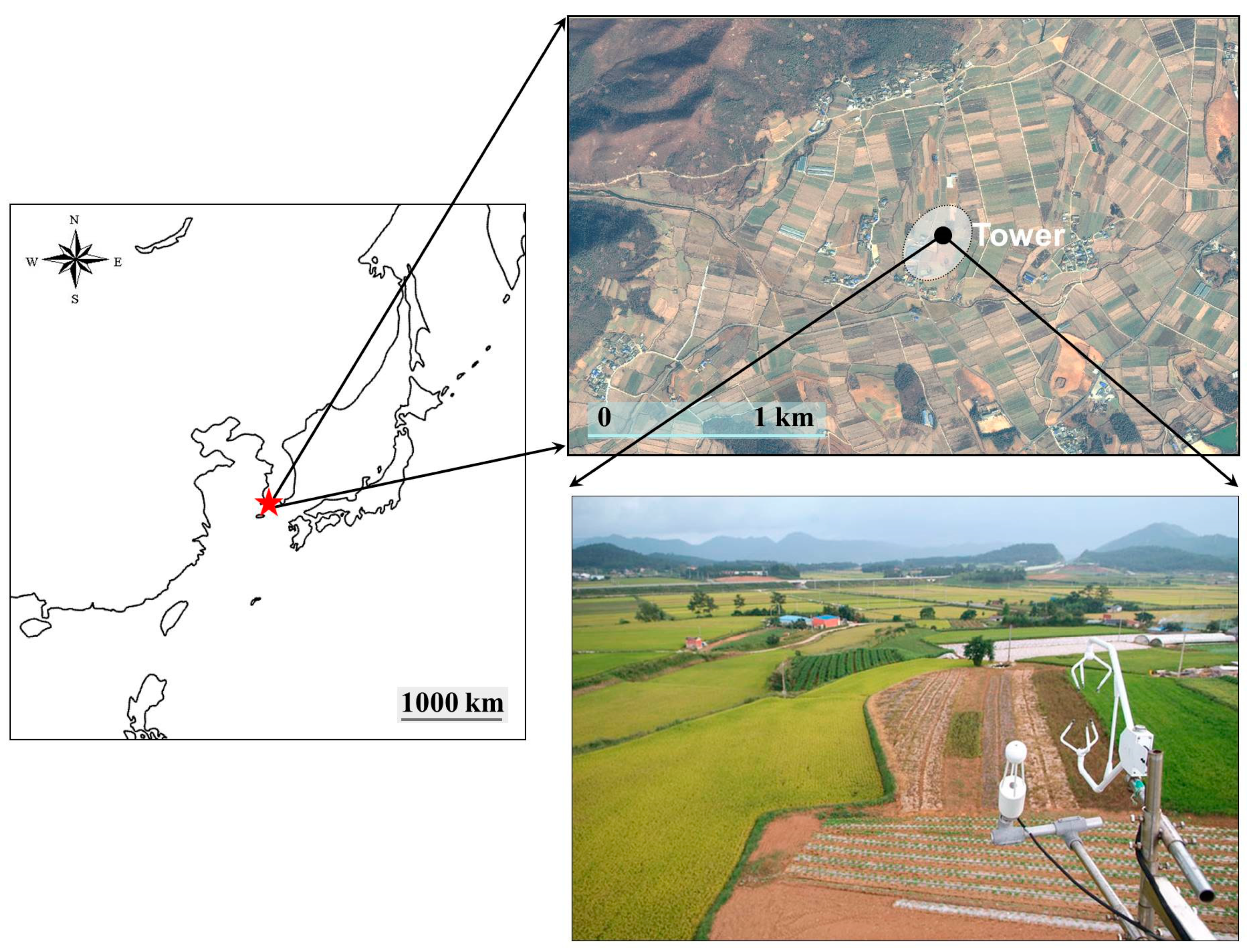
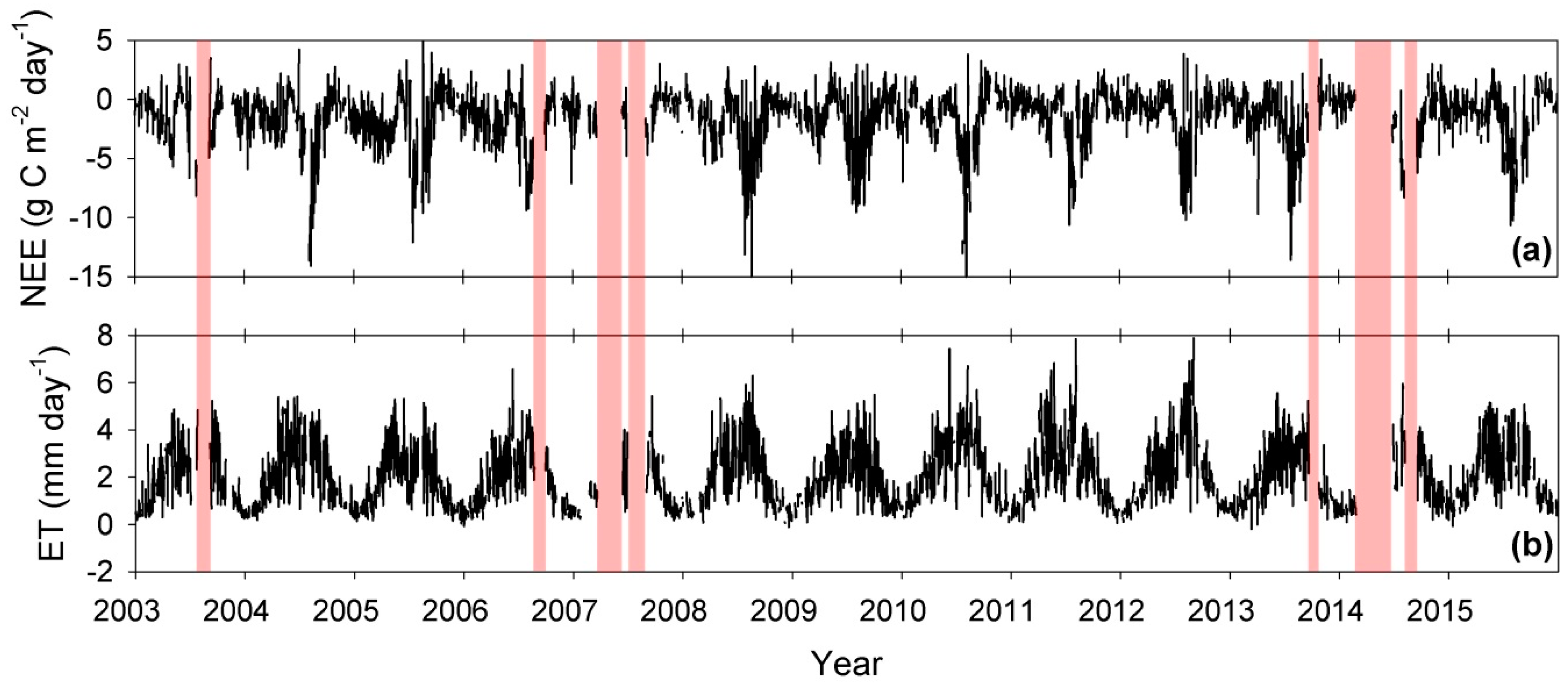
2.1. Site and Data Description

The HFK site is located near the southwestern coast of the Korean Peninsula (34°33′14′′ N, 127°34′12′′ E, 12 m a.s.l.; Figure 2). The major vegetation near the tower (within ~300 m) is seasonally cultivated crops such as beans, sweet potatoes, Indian millet, and sesame. Beyond this area, rice paddies prevail, except in the northern area. The HFK site practices two-crop rotation in the same area in sequential seasons (i.e., rice for summer and fall and barley for spring). A detailed description of the HFK site has been given previously by Lee et al. [9].

The EC technique is used to measure the CO₂/H₂O/energy fluxes from a 20 m tower at the site. Vertical and horizontal wind speeds and temperature are measured with a three-dimensional sonic anemometer and thermometer (SAT; Model CSAT3, Campbell Scientific Inc., Logan, UT, USA) at 10 Hz. An open-path infrared gas analyzer (IRGA; Model LI-7500, LI-COR Inc., Lincoln, NE, USA) is used to measure CO₂ and H₂O concentrations. Half-hourly ECs and the associated statistics are calculated online from the 10 Hz raw data and stored in a datalogger (Model CR5000, Campbell Scientific Inc., Logan, UT, USA). The ECs are corrected in the post-processing phase (a sector-wise planar fit rotation producing eight tilt planes every 28 days [11,12,13] and Webb–Pearman–Leuning correction [14]). Other measurements such as net radiation, air temperature, humidity, soil temperature, ground heat fluxes, and soil water content are sampled every 10 s, averaged over 30 min, and logged in the datalogger. More information about EC and these meteorological measurements can be found in Kwon et al. [15].

To improve the data quality by eliminating data that is physiologically and physically implausible, the collected data are examined by a quality control procedure based on the KoFlux data-processing protocol [16,17]. This procedure includes storage term calculation [18], spike detection [18], gap-filling (by marginal distribution sampling method that is appropriate for gaps of less than a month [1]), and nighttime CO₂ flux correction [19]. For gap-filling of meteorological data (e.g., downward shortwave radiation, air temperature, humidity, and precipitation), linear interpolation is applied for short (<4 h) gaps and linear regression is performed using data from the automated synoptic observing system operated by the Korea Meteorological Administration, which is located about 100 m from the flux tower. The distribution of long gaps in the meteorological data was similar to that in the flux data.

After quality control (and before gap-filling), the final percentage of data retrieval was 59 ± 12% for CO₂ flux and 61 ± 12% for ET over the study period from 2003 to 2015 (

Table 1. Annual data retrieval rates, lengths of the first and second longest gaps, and total lengths of the long gaps ¹ for CO₂ flux (F_CO2) and evapotranspiration (ET) from 2003 to 2015 for the study site. AVG denotes average; STD denotes standard deviation.

Year	Data Retrieval Rate (%)		Length of the 1st Longest Gap (Day)		Length of the 2nd Longest Gap (Day)		Total Length of the Long Gaps (Day)
	FCO2	ET	FCO2	ET	FCO2	ET	FCO2	ET
2003	52.3	55.9	34.3	34.3	23.0	23.0	34.3	34.3
2004	68.1	69.4	13.1	13.0	1.4	1.5	0.0	0.0
2005	69.8	72.0	13.4	13.4	1.5	2.2	0.0	0.0
2006	60.7	62.4	35.3	35.3	20.5	20.5	35.3	35.3
2007	34.6	35.7	82.5	81.5	61.4	61.4	143.9	142.9
2008	62.5	67.1	13.9	13.8	4.8	4.7	0.0	0.0
2009	61.9	63.0	4.8	4.8	2.9	2.9	0.0	0.0
2010	64.5	67.2	4.1	3.9	3.3	3.2	0.0	0.0
2011	71.1	70.6	2.6	2.7	2.4	2.4	0.0	0.0
2012	65.1	67.3	7.6	7.5	2.9	2.1	0.0	0.0
2013	63.3	65.5	31.3	31.2	1.7	1.7	31.3	31.2
2014	35.5	36.2	123.1	123.1	41.1	41.1	164.1	164.1
2015	63.4	63.4	12.4	12.4	3.1	3.1	0.0	0.0
AVG 2	59.4	61.2	29.1	29.0	13.1	13.1	31.5	31.4
STD	11.8	11.9	35.5	35.4	18.8	18.8	56.4	56.4

¹ Longer than 30 days; ² The average values (%) of F_CO2 and ET were 63.9 and 65.8, respectively, for the study period except 2007 and 2014, and were 35.1 and 35.9 for 2007 and 2014, respectively.

). The data retrieval rates for CO₂ flux and ET were relatively low because the open-path IRGA measurements were frequently impaired by sea fog (the site is located near the sea). The data retrieval rates were ~35% in 2007 and 2014, somewhat lower than in other years (~65%). The first and second longest gaps in 2007 and 2014 lasted 82 and 61, and 123 and 41 days, respectively. The total lengths of the long gaps (i.e., longer than 30 days) were 143 days in 2007 and 164 days in 2014.

The CO₂ flux manifested bimodal peaks that occurred first in May (the most vigorous growing period of barley) and later in August (the most vigorous growing period of rice) for the other years (see Figure 1). It is hard to reliably quantify the seasonal variation and annual budgets of CO₂ in 2007 and 2014. Except for 2007 and 2014, we filled the flux data gaps using the marginal distribution sampling method. For nighttime CO₂ flux correction and partitioning NEE into GPP and RE, we applied the friction velocity (u^*) correction method with the modified moving point test method for determining u^* threshold [19], and extrapolated nighttime values of RE into the daytime values using the RE equation with a short-term (air) temperature sensitivity of RE from the nighttime data [1]. GPP was calculated by subtracting NEE from RE.

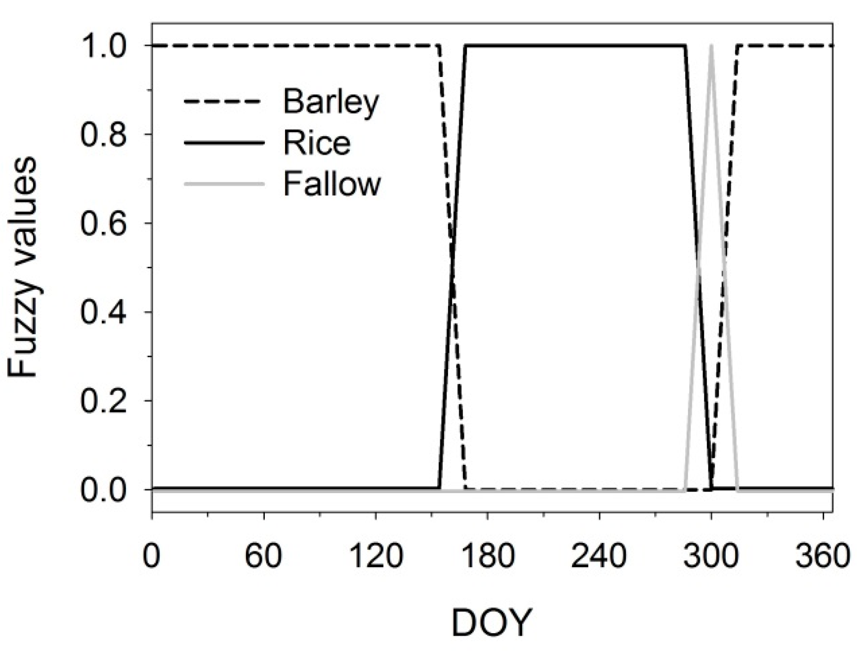
2.2. Data-Driven Approach Using Support Vector Regression and Its Modification

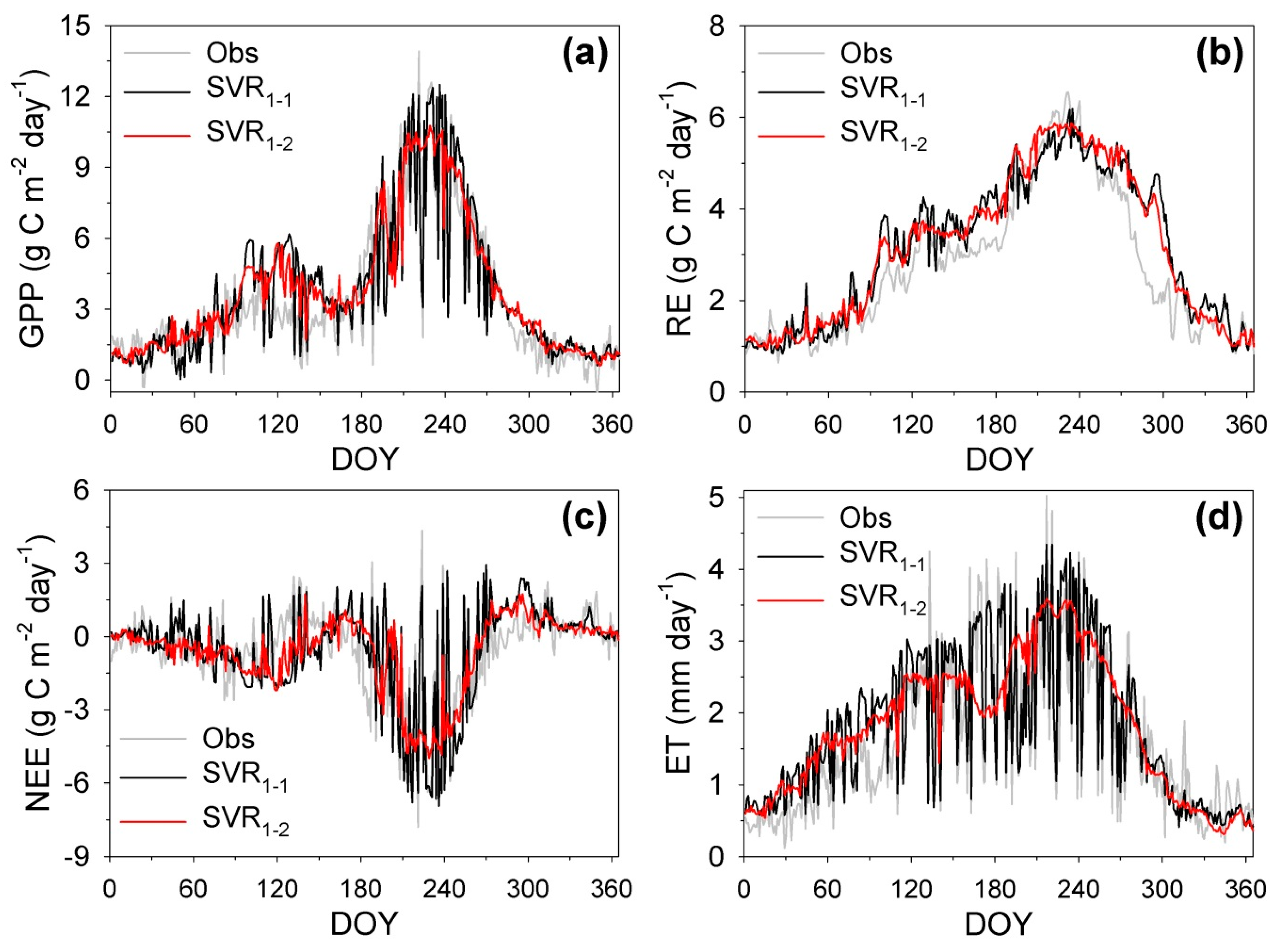
In this study, we used a data-driven methodology using remote-sensing data and support vector regression (SVR) [8], which has been demonstrated in the estimation of terrestrial CO₂ fluxes in Asia. SVR is a machine learning technique that transforms nonlinear regressions into linear regressions. It includes a data classification process that maps the original low-dimensional input space to a higher-dimensional feature space for classifying the data linearly e.g., [20]. This method first sets up an empirical model using site observational data and explanatory variables, and then applies the established model to generate extensive spatial data for continental-scale applications. Similarly, we were able to set up a model using one site’s observational data, and then predict time-series data to fill long gaps using the model. Detailed information about SVR can be found in Ichii et al. [21]. LIB-SVM software was used to implement the SVR [22] (http://www.csie.ntu.edu.tw/~cjlin/libsvm/).

To apply the data-driven approach to the filling of long gaps in flux data, we modified the methodology as follows. First, we set the temporal scale of interest from days to multi-year. The target variables were daily integrated GPP (g C m⁻² day⁻¹), RE (g C m⁻² day⁻¹), NEE (g C m⁻² day⁻¹), and ET (mm day⁻¹), whereas the input variables were the daily downward shortwave radiation (R_sdn, MJ m⁻² day⁻¹), daytime air temperature (T_air, °C), daytime vapor pressure deficit (VPD, hPa) and precipitation (P, mm day⁻¹) at the flux tower, and the leaf area index (LAI, m² m⁻²; [23]), enhanced vegetation index (EVI, unitless; [24]), and land–surface water index (LSWI, unitless; [25]) from the eight-day moderate resolution imaging spectroradiometer (MODIS) data products (MOD15A2 and MCD43A4 version 6; [26] https://daac.ornl.gov/LAND_VAL/guides/MODIS_Web_Service_C6.html). The LAI, EVI, and LSWI data had a grid size of 1.5 km (i.e., 3 × 3 pixels) and were linearly interpolated to daily values under the assumption that day-to-day fluctuations of these indices were small. Additionally, a fuzzy transform was applied to the cultivation, assigning fuzzy values of 0–1 to barley, rice, and fallow, to distinguish each ecosystem state; this was similar to the procedure used by Papale and Valentini [27] (Figure 3). From the perspective of ecological processes, NEE was not directly estimated using machine learning, but was instead calculated by subtracting the estimated GPP from the estimated RE.

To understand the microclimatology and ecosystem state of the study site, we briefly examined the seasonality and annual sums (or means) of the input variables (Figures S1 and S2,

Table 2. Annual values of integrated (or averaged) downward shortwave radiation (R_sdn), daytime air temperature (T_air), daytime vapor pressure deficit (VPD), precipitation (P), leaf area index (LAI), enhance vegetation index (EVI), and land–surface water index (LSWI) from 2003 to 2015 for the study site. AVG denotes average; STD denotes standard deviation.

Year	Rsdn	Tair	VPD	P	LAI	EVI	LSWI
	(MJ m−2)	(°C)	(hPa)	(mm)	(m2 m−2)	(Unitless)	(Unitless)
2003	4750	15.8	6.6	1740	0.96	0.30	0.10
2004	5190	16.5	8.6	1594	0.99	0.30	0.08
2005	5298	15.8	7.0	1272	0.92	0.29	0.08
2006	4909	15.9	7.0	1683	0.89	0.29	0.09
2007	4833	16.2	7.3	1678	0.94	0.30	0.09
2008	5100	16.1	7.3	1098	0.91	0.28	0.08
2009	5186	15.9	7.2	1278	0.99	0.30	0.10
2010	4897	15.2	6.3	1496	0.94	0.30	0.10
2011	5147	14.8	6.2	1499	0.85	0.29	0.08
2012	5107	14.8	6.2	1695	0.78	0.29	0.09
2013	5319	15.4	6.1	1078	0.89	0.29	0.07
2014	5082	15.5	5.7	1173	0.93	0.31	0.10
2015	5162	15.7	5.6	1158	0.89	0.29	0.09
AVG	5075	15.7	6.7	1419	0.91	0.29	0.09
STD	176	0.5	0.8	250	0.06	0.01	0.01

). A feature worth noting was a mid-season depression in R_sdn due to “changma”, i.e., an intensive rainy spell that occurs during the summer [10,15]. The highest T_air was ~30 °C in early August, while the lowest T_air was ~−3 °C in January. The VPD seasonally changed with T_air and P, and there was also a mid-season depression, similarly to R_sdn. The variations of LAI, EVI, and LSWI were related to the cultivation (i.e., two-crop rotation). The averages of annual sums (or means) during the study period were 5075 ± 176 (average ± one standard deviation) MJ m⁻² year⁻¹ for R_sdn, 15.7 ± 0.5 °C for T_air, 6.7 ± 0.8 hPa for VPD, 1254 ± 229 mm year⁻¹ for P, 0.91 ± 0.06 m² m⁻² for LAI, 0.29 ± 0.01 for EVI, and 0.09 ± 0.01 for LSWI. Note that the lowest annually-averaged T_air and LAI (14.8 °C and 0.78 m² m⁻², respectively) occurred simultaneously in 2012, while both were the highest (16.5 °C and 0.99 m² m⁻², respectively) in 2004.

To determine appropriate gap-filling strategies, we tested the following three hypotheses: (1) Estimation using in situ meteorological measurement data as input data to SVR is more reasonable than that using remote-sensing (or modeling) data; (2) A closer (to gaps) training dataset for machine learning results in better estimation; and (3) A longer training dataset for machine learning results in better estimation. To test these hypotheses, we designed experiments to target the flux data in 2009 because it was the middle of the database (

Table 3. Hypotheses and experimental design.

Hypotheses	Exp. No.	Target Year	Training Year	Meteorological Input Source
(1) Estimation using in situ measurement data as the input for machine learning is more reasonable than that using remote-sensing and modeling data.	1-1	2009	2008 & 2010	In situ measurement
	1-2			Remote sensing & modeling
(2) A training dataset for machine learning that is closer to the gaps results in better estimation.	2-1	2009	2008 & 2010	In situ measurement
	2-2		2006 & 2011
	2-3		2005 & 2012
	2-4		2004 & 2013
	2-5		2003 & 2015
(3) A longer training dataset for machine learning results in better estimation.	3-1	2009	2008 or 2010	In situ measurement
	3-2		2008 & 2010
	3-3		2006, 2008, 2010, & 2011
	3-4		2005, 2006, 2008, 2010, 2011, & 2012
	3-5		2004, 2005, 2006, 2008, 2010, 2011, 2012, & 2013
	3-6		2003, 2004, 2005, 2006, 2008, 2010, 2011, 2012, 2013, & 2015

). All the SVR-based models estimated the fluxes in 2009, and the original gap-filled data in 2009 from the marginal distribution sampling method were used for their validation. In addition, to test Hypothesis 1, we obtained the eight-day daytime land surface temperature (LST) from the MODIS data products (MOD11A2 version 6; [28]), the daily daytime vapor pressure deficit and precipitation from the reanalysis data [29], with adjustments based on the meteorological observations at each site, and the daily downward shortwave radiation (SWR) from the Japan Aerospace Exploration Agency (JAXA) Satellite Monitoring for Environmental Studies product ([30]; http://kuroshio.eorc.jaxa.jp/JASMES/index.html); these data have been used for the estimation of terrestrial CO₂ fluxes in Asia [8]. The eight-day LST data were temporally interpolated to daily data based on the daytime air temperature from the reanalysis data. Detailed information about the inputs from remote-sensing and modeling data can be found in Ichii et al. [8,29].

3. Results

Table 4. Statistical parameters for error assessment of Experiments 1-1 and 1-2. MBE and RMSE indicate mean bias error and root-mean-square error, respectively. Slope and r² were obtained from linear regression analysis¹. GPP, RE, NEE, and ET represent the daily gross primary production, ecosystem respiration, net ecosystem exchange, and evapotranspiration, respectively. Numbers in bold indicate the best estimations based on each of the statistical parameters for error assessment.

Variables	Experiment No. 1-1				Experiment No. 1-2
	MBE	RMSE	Slope	r2	MBE	RMSE	Slope	r2
GPP (g C m−2 day−1)	0.441	1.204	1.070	0.841	0.518	1.545	1.028	0.679
RE (g C m−2 day−1)	0.373	0.717	1.086	0.819	0.376	0.655	1.100	0.875
NEE (g C m−2 day−1)	−0.068	1.156	0.948	0.653	−0.142	1.463	0.585	0.294
ET (mm day−1)	0.225	0.457	1.081	0.832	0.228	0.761	0.997	0.328

¹ We performed linear regression analysis instead of orthogonal (or major axis) regression analysis even though the observational data from 2009 (the target year) also had uncertainties. For error assessment, we implicitly assumed that the uncertainties of measured data were negligible when we set up a support vector regression (SVR)-based model using the observational data.

presents the results of Experiments 1-1 and 1-2, which supported Hypothesis 1, that is, estimation using in situ measurement data as the (meteorological) input to machine learning is more reasonable than using remote-sensing and modeling data. The actual measurement data should be more reliable than the remote-sensing and modeling data. For example, the footprints of EC flux data (size: <1 km) were matched with those of the in situ measurement data (<1 km), rather than the remote-sensing grid (LST: 3 km; SWR: 5 km) and modeling data (~250 km). Considering the spatial heterogeneity of the study site, we expected the SVR-based model from Experiment 1-1 to outperform the one from Experiment 1-2 e.g., [31]. The estimations using both the in situ measurement data and remote-sensing (and modeling) data agreed reasonably well with the observations (Figure 4, except for the ET from Experiment 1-2 around DOY (day of year) 180). As expected, the day-to-day fluctuations of estimations using remote-sensing and modeling data were significantly smaller than those of the observations, resulting in higher root-mean-square errors (RMSE) and lower coefficients of determination (r²) than those for the estimations using the in situ measurement data, except for the RE with small actual day-to-day variations.

Based on the results of Experiments 2-1 to 2-5 (Figure 5), we rejected Hypothesis 2, that is, that a training dataset for machine learning closer to the gaps would result in better estimation. We expected that using the closest training dataset would give the best results for Experiment 2-1, because the ecosystem state of the target year might be similar to that of the training years. Contrary to this expectation, the results of Experiment 2-1 were not the best except the RMSE for ET, and there were no increasing (decreasing) trends of the RMSE (r²) with the amount of time elapsed between the target year and the training year.

On the basis of the results for Experiments 3-1 to 3-6 (Figure 6), we accepted Hypothesis 3, that is, that a longer training dataset for machine learning would result in better estimation. We expected the experimental results to improve as the training datasets became longer. Considering that extrapolation (interpolation) involves predicting a value outside (inside) the domain of the data, extrapolation is more uncertain than interpolation. If the domain is extended with the length of the training dataset, the gap-filling is closer to interpolation (with less uncertainty) than extrapolation. As expected, using longer datasets for training produced better estimations (i.e., lower RMSE and higher r²) by gradually reducing the discrepancies between the observations and the SVR-based model (Figures S3 and S4). It is worth noting that GPP improved quite a lot with Experiment 3-4 (Experiment 3-5), probably because the model included the data in 2012 and 2004, when the lowest and highest annually-averaged T_air and LAI occurred simultaneously, respectively (see Table 2).

4. Discussion

Before discussing the uncertainty and interannual variability issues, we examined the uncertainty related to the selection of the gap-filling method through a comparison with other models.

Table 5. Statistical parameters for error assessment of Experiment 3-6 using SVR, random forest (RF), and artificial neural network (ANN). MBE and RMSE indicate mean bias error and root-mean-square error, respectively (Units: g C m⁻² day⁻¹ for GPP, RE and NEE, mm day⁻¹ for ET). Slope and r² obtained from linear regression analysis. Numbers in bold indicate the best estimations based on each of the statistical parameters for error assessment.

Variables	Support Vector Regression				Random Forest				Artificial Neural Network
	MBE	RMSE	Slope	r2	MBE	RMSE	Slope	r2	MBE	RMSE	Slope	r2
GPP	0.335	0.925	1.045	0.896	0.412	0.940	1.046	0.885	0.338	0.938	1.050	0.895
RE	0.337	0.568	1.086	0.899	0.454	0.628	1.133	0.922	0.376	0.633	1.100	0.876
NEE	0.002	0.892	0.941	0.763	0.043	0.854	0.825	0.753	0.038	0.895	0.949	0.767
ET	0.229	0.477	1.105	0.854	0.252	0.474	1.096	0.831	0.240	0.477	1.095	0.833

presents the results of Experiment 3-6 using SVR and other machine learning techniques, i.e., random forest (RF) and artificial neural network (ANN). The randomForest R package was used to implement the RF [32] (https://www.rdocumentation.org/packages/randomForest/versions/4.6-14/topics/randomForest), and the Neural Network Fitting application of MATLAB^® was used to implement the ANN [33] (https://www.mathworks.com/help/deeplearning/gs/fit-data-with-a-neural-network.html). The number of trees and the number of variables tried at each split for the RF were respectively 1000 and 3, while the number of hidden neurons for the ANN was 10. The SVR-based model performed similarly to the RF- and ANN-based models, suggesting that the uncertainty related to the selection of the machine learning technique was relatively small. Thus, we estimated the fluxes using the SVR-based model trained with all available data except for 2007, 2014, and the target year to answer the following two questions: “How large is the uncertainty related to the long-period flux-gap-filling?” and “Can the long-period-gap-filled flux data capture the interannual variability?”

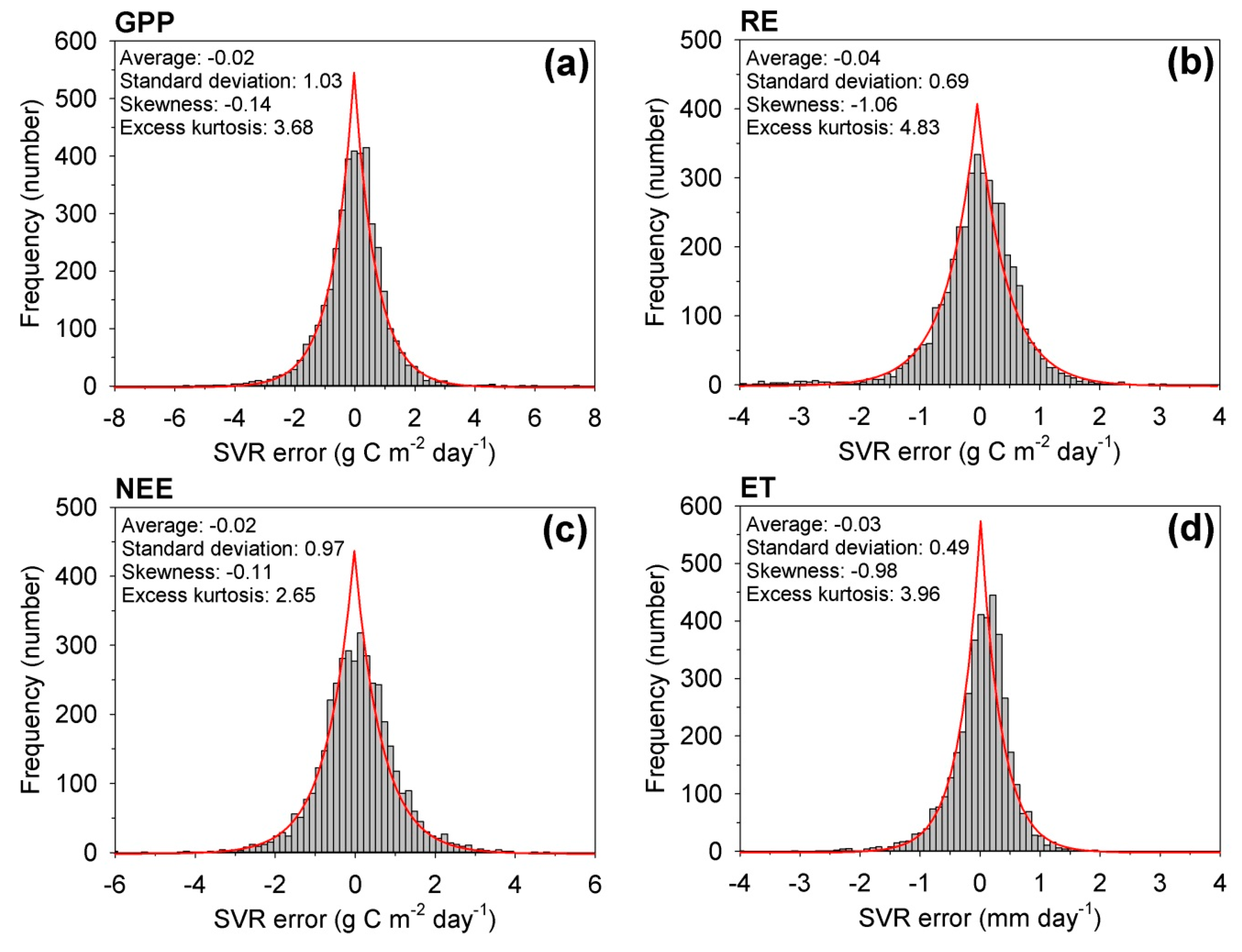
4.1. How Large is the Uncertainty Related to the Long-Period Flux-Gap-Filling?

The error in the long-period flux-gap-filling exhibited a double-exponential (Laplace) distribution, similarly to the random flux measurement error e.g., [34]. Figure 7 shows histograms of the SVR model (i.e., SVR-based model trained using all available data except for 2007, 2014, and the target year, hereafter called SVR_all) error for the fluxes (= estimation using SVR_all − gap-filled data using the marginal distribution sampling method) and the statistics that explain their distributions over the entire study period. The averages were close to 0, whereas the standard deviations ranged from 0.49 to 1.03. The distributions were slightly left-skewed. The excess kurtoses ranged from 2.65 to 4.83, indicating that the distributions were fitted to a double-exponential distribution (with excess kurtosis of 3) rather than a normal distribution (with excess kurtosis of 0).

To quantify the uncertainties in the annual flux sums due to the long-period flux-gap-filling, we used a standard Monte Carlo approach [35]. First, we added artificial noise into the flux dataset to account for the SVR model errors. The noise was generated from a double-exponential distribution with a suitable standard deviation for each cultivation season (i.e., rice cultivation and non-rice cultivation), which was estimated similarly to Figure 7. We repeated this process 100 times, and then calculated the standard deviation of the annual sums (σ). The factor 2σ represents the uncertainty in the annual flux sum due to the long-period flux-gap-filling at approximate 95% confidence intervals. The values of 2σ were approximately 57 g C m⁻² year⁻¹ in GPP, 37 g C m⁻² year⁻¹ in RE, 52 g C m⁻² year⁻¹ in NEE, and 27 mm year⁻¹ in ET. Compared with the random flux measurement uncertainties (29 g C m⁻² year⁻¹ in GPP, 40 g C m⁻² year⁻¹ in RE, 25 g C m⁻² year⁻¹ in NEE, and 5.2 mm year⁻¹ in ET, quantified according to Finkelstein and Sims [36] and Richardson and Hollinger [35]), the uncertainties in GPP, NEE, and ET due to the long-period flux-gap-filling were much higher than those due to random sampling, whereas the uncertainties related to the selection of the machine learning technique (32 g C m⁻² year⁻¹ in GPP, 43 g C m⁻² year⁻¹ in RE, 16 g C m⁻² year⁻¹ in NEE, and 8.4 mm year⁻¹ in ET) were comparable to the random flux measurement uncertainties. As expected, the uncertainty in annual NEE due to the long-period flux-gap-filling was almost twice as high as the additional uncertainty of 30 g C m⁻² year⁻¹ caused by a week-long gap during spring green-up in a deciduous forest (with mean annual GPP of 1339 g C m⁻² year⁻¹, RE of 1165 g C m⁻² year⁻¹, and NEE of −174 g C m⁻² year⁻¹) when traditional nonlinear models (derived from single-year data) were applied for gap-filling [35].

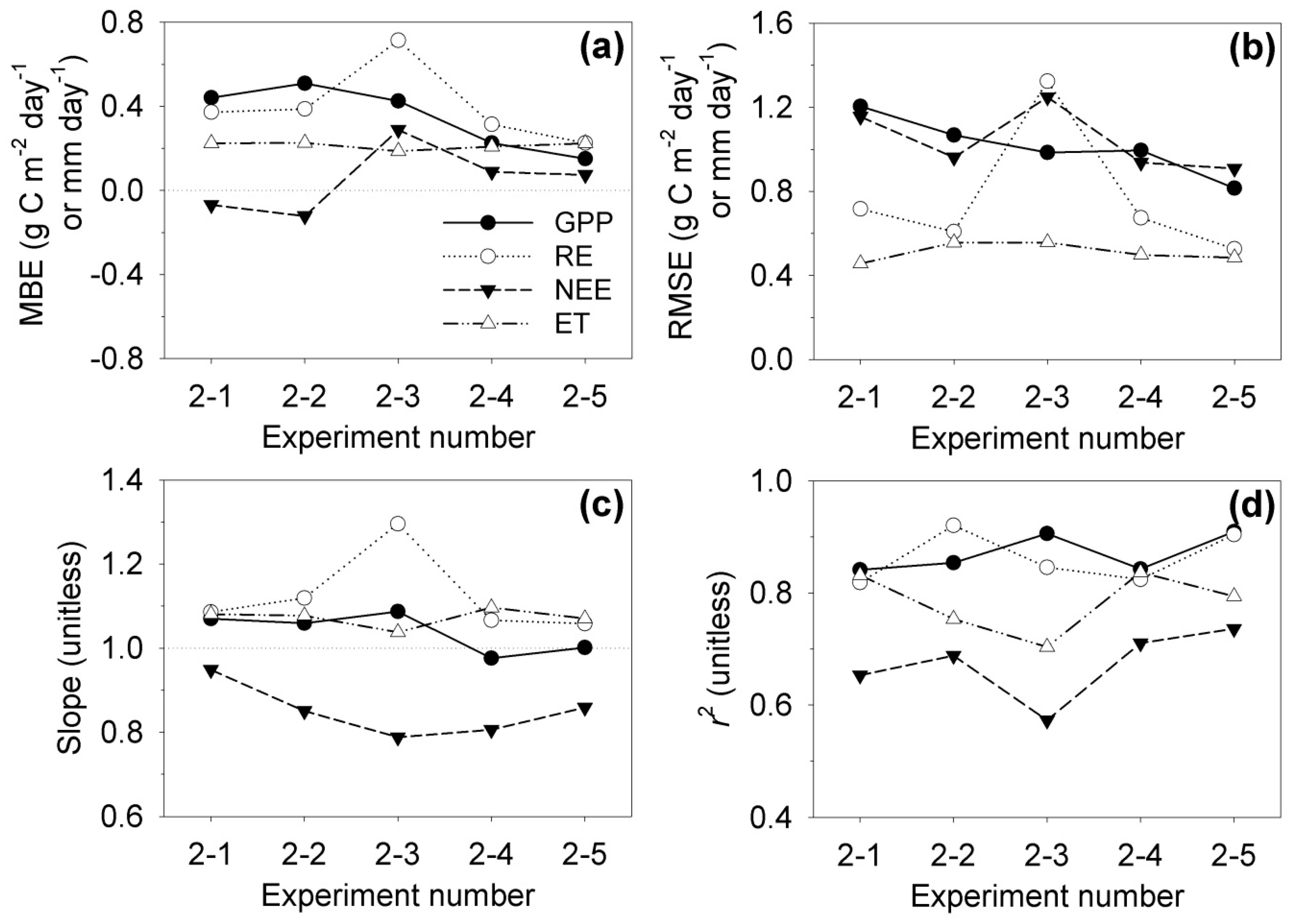
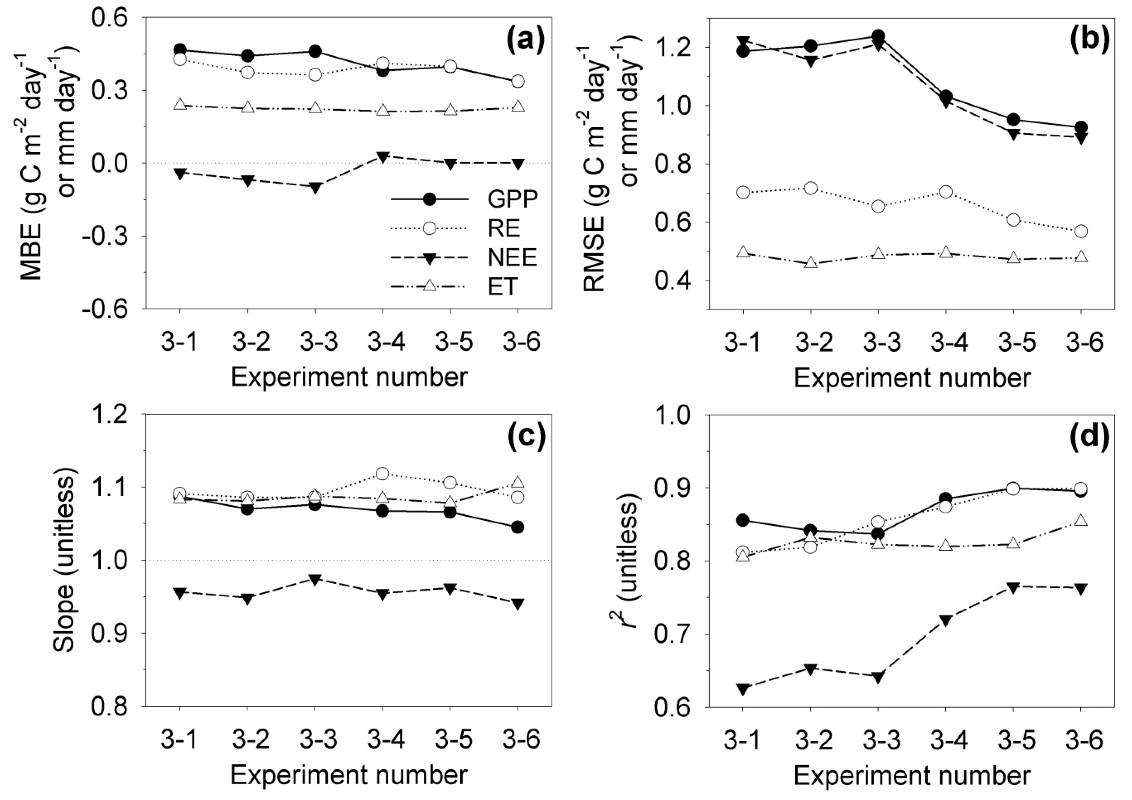
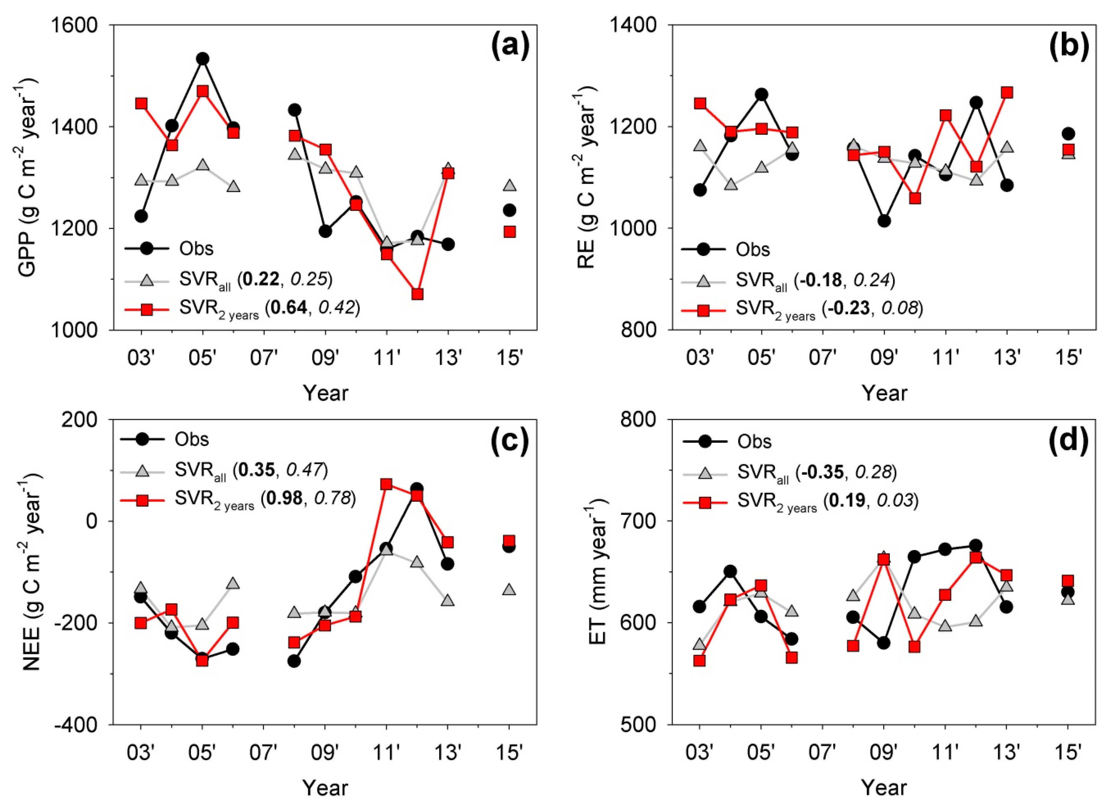
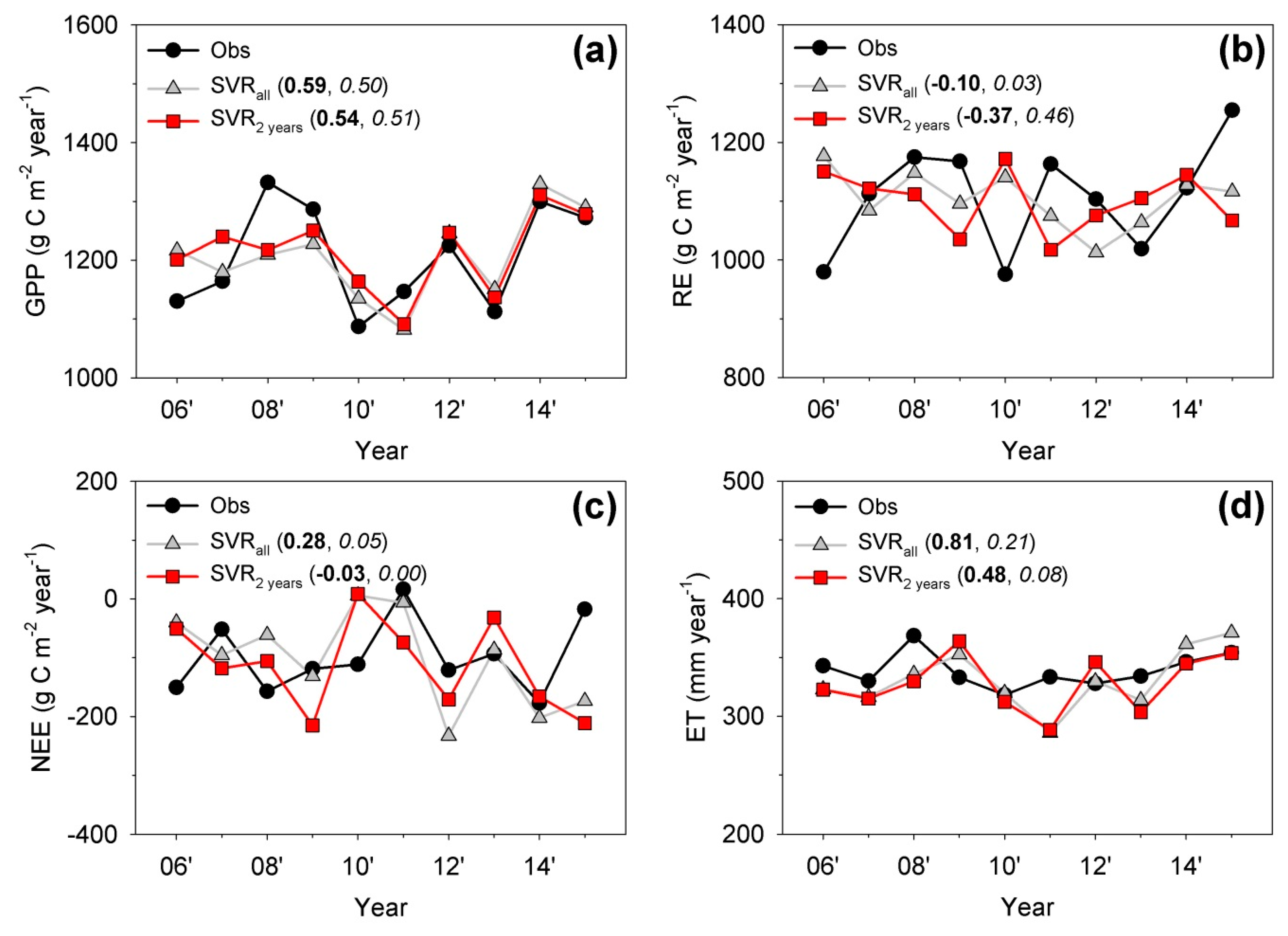
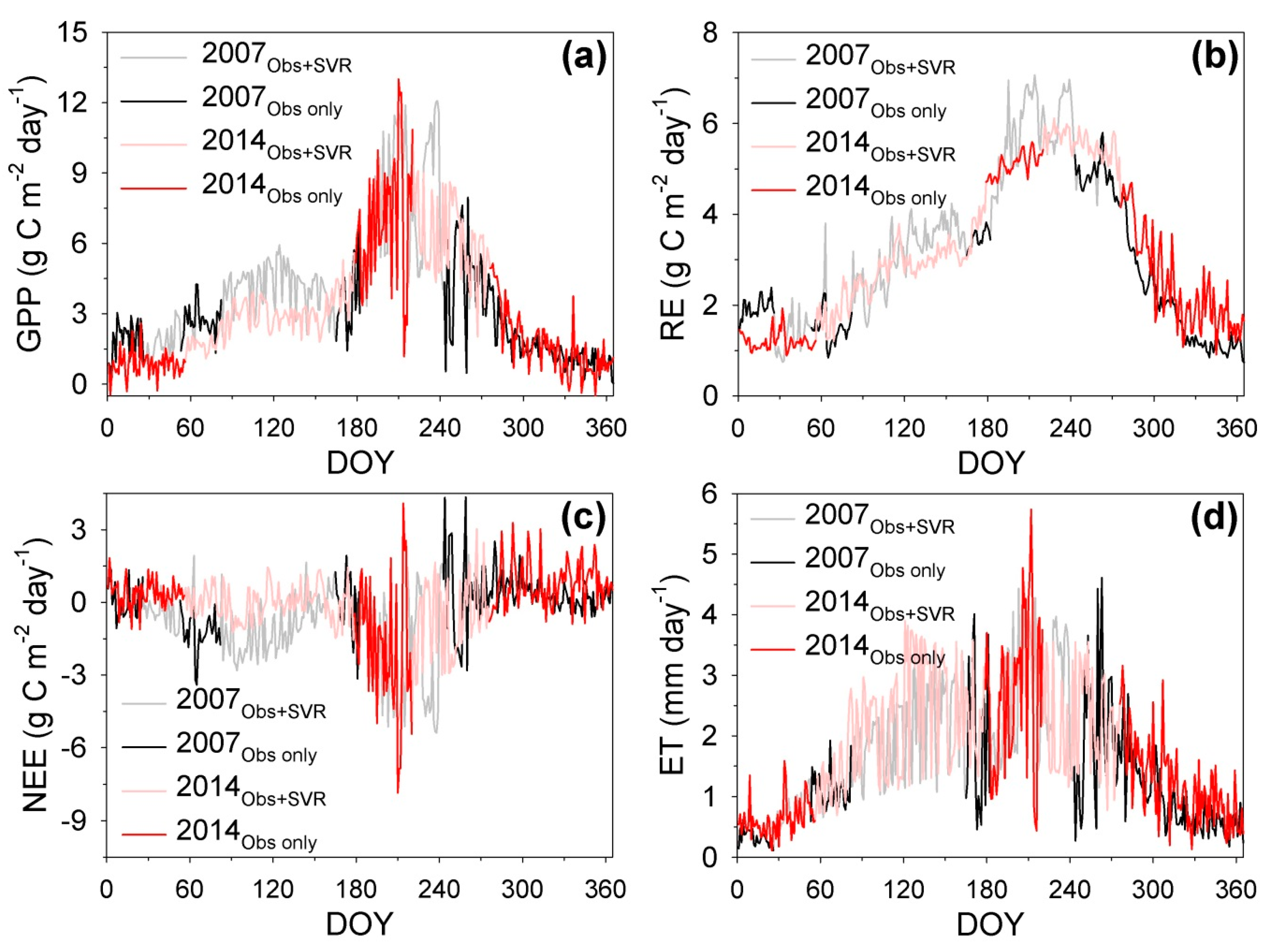
4.2. Can the Long-Period-Gap-Filled Flux Data Capture the Interannual Variability?

We found considerable discrepancies in interannual variability between the SVR_all and the observations (Figure 8), even though the model performance for seasonality was excellent. We also estimated the uncertainties in annual sums introduced by the gap-filling approach by determining the standard deviation of the differences between modeled and measured annual fluxes in Figure 8. The standard deviations were 112 g C m⁻² year⁻¹ for GPP, 91 g C m⁻² year⁻¹ for RE, 83 g C m⁻² year⁻¹ for NEE, and 50 mm year⁻¹ for ET, which were almost twice as high as the uncertainties previously quantified using the Monte Carlo approach. This supports the idea that it is more difficult to capture the interannual variability than the seasonal variability. For RE and ET, in particular, the estimations from SVR_all and the observations were negatively correlated. Note that the interannual variability derived from SVR_all was much smaller than that from the observations. Micro-/bio-meteorological phenomena can be described as cycles composed of various processes with different time scales, e.g., day, season, year, several years/decades, century, millennium. Most gap-filling methods are based on the fact that similar phenomena happen repeatedly as time passes [5]. Such repeatability decreases exponentially with the length of the time scale, highlighting the difficulty of predicting very long variations such as interannual variability. There is also a possibility that the observations could not capture the cycles that determined the interannual variability (lack of temporal representativeness [37]).

The discrepancies could be improved by training the SVR-based model using data from the closest two years around the target year, i.e., previous year and following year except for 2007 and 2014 (SVR_{2 years}). This suggests that using longer datasets for training generally produces better model performance, but there is a greater possibility that interannual variations caused by ecosystem state changes (e.g., changes in crop variety and cultivation area) will not be captured. Indrawati et al. [38] reported that four different varieties of rice (Dongjin No. 1 (2003–2008), Nampyung (2009), Onnuri (2010–2011), and Saenuri (2012–2015)) were cultivated at the site, each having different efficiency in terms of water/light/carbon use. This change will have lowered the predictability of SVR_all. It is challenging to consider such changes in variety, as far more data are required for training the model. Additionally, in the case of barley cultivation, the cultivation area changed considerably every year at the site (Korean Statistical Information Service, http://kosis.kr/eng/).

To strengthen our inference, we also tested the flux data (without long gaps, Table S1) measured at the Gwangneung deciduous forest in the Korea National Arboretum (GDK; 37°44′56′′ N, 127° 8′57′′ E, 252 m a.s.l.) [17,39]. Gwangneung is a royal forest that surrounds the mausoleum of King Sejo of the Joseon dynasty. Hence, over the last 550 years, this area has been protected to minimize human disturbance [40]. Unlike at the HFK site, SVR_all outperformed SVR_{2 years}, supporting our inference (Figure 9). The estimations and observations of RE were again negatively correlated. We speculated that the poor predictability of RE may have been because we overlooked a driver that controls the interannual variability, such as supplements of organic matter (e.g., manure, residues after harvest, litter, deadwood). Our results suggests that the performance of short-, mid-, or long-term training might vary from site to site, and thus further scrutinization of the ideal training length should be inferred from a multi-site study, or needs to be evaluated for each site separately.

In accordance with the results and discussion, we estimated the daily fluxes in 2007 and 2014 using the SVR_{2 years} model trained by in situ measurement data for long-period-gap-filling of the HFK site, and then replaced the original gap-filled data from the marginal distribution sampling method with the estimated data using SVR_{2 years} when the daily data retrieval rate of 0% lasted more than a month (Figure 10). The RMSEs of the SVR_{2 years} in 2007 and 2014 quantified using the available measured data were 0.839 g C m⁻² day⁻¹ for GPP, 0.503 g C m⁻² day⁻¹ for RE, 0.745 g C m⁻² day⁻¹ for NEE, and 0.392 mm day^-1 for ET, which were comparable to those from Experiment 3-6. The final annual sums with uncertainty related to the long-period flux-gap-filling (2σ, quantified using the Monte Carlo approach) for 2007 (2014) were 1347 ± 58 (1174 ± 62) g C m⁻² year⁻¹ for GPP, 1129 ± 40 (1146 ± 51) g C m⁻² year⁻¹ for RE, −217 ± 60 (−28 ± 57) g C m⁻² year⁻¹ for NEE, and 587 ± 29 (639 ± 29) mm year⁻¹ for ET. Since the mean bias errors of the SVR_{2 years} in 2007 and 2014 were close to 0, the annual sums were almost identical whether we included the measured data or not. Despite the long gaps of 143–164 days, the uncertainties except for NEE were less than 5% of the annual sums.

5. Conclusions: Gap-Filling Strategies for Long-Period Flux Data Gaps

Based on the results and discussion, we propose the following gap-filling strategies for long-period flux data.

• In situ measurement data should be preferentially used as the input for machine learning, if available.
• Data covering as long a period as possible should be used to train the machine-learning-based model.
• If there has been a significant ecosystem state change over the study period and the primary objective of gap-filling is to quantify interannual variability rather than seasonality, multiple models should be established for each ecosystem state.

If in situ measurements are not available, there is no choice but to use remote-sensing or modeling data. In such a case, we recommend the temporal resolution of the machine-learning-based model be increased (e.g., one-day to eight-day). In a follow-up study, we will develop methodologies to establish a machine-learning-based model trained using all data, giving weight to the data close to the gaps and considering a time lag between fluxes and drivers (e.g., the relationship between vegetation greenness and GPP [41]). Our findings in this paper emphasized the validity of the long-term database for both gap-filling and the estimation of terrestrial CO₂/H₂O fluxes using a data-driven approach. Particularly, they support the idea that the relationships between fluxes and their drivers can change in the long term, implying the necessity for continuous measurements to understand such changes.

References

1. Reichstein, M.; Falge, E.; Baldocchi, D.; Papale, D.; Aubinet, M.; Berbigier, P.; Bernhofer, C.; Buchmann, N.; Gilmanov, T.; Granier, A.; et al. On the separation of net ecosystem exchange into assimilation and ecosystem respiration: Review and improved algorithm. Glob. Chang. Biol. 2005, 11, 1424–1439. [Google Scholar] [CrossRef]
2. Falge, E.; Baldocchi, D.; Olson, R.; Anthoni, P.; Aubinet, M.; Bernhofer, C.; Burba, G.; Ceulemans, R.; Clement, R.; Dolman, H.; et al. Gap filling strategies for long term energy flux data sets. Agric. For. Meteorol. 2001, 107, 71–77. [Google Scholar] [CrossRef] [Green Version]
3. Falge, E.; Baldocchi, D.; Olson, R.; Anthoni, P.; Aubinet, M.; Bernhofer, C.; Burba, G.; Ceulemans, R.; Clement, R.; Dolman, H.; et al. Gap filling strategies for defensible annual sums of net ecosystem exchange. Agric. For. Meteorol. 2001, 107, 43–69. [Google Scholar] [CrossRef] [Green Version]
4. Moffat, A.M.; Papale, D.; Reichstein, M.; Hollinger, D.Y.; Richardson, A.D.; Barr, A.G.; Beckstein, C.; Braswell, B.H.; Churkina, G.; Desai, A.R.; et al. Comprehensive comparison of gap-filling techniques for eddy covariance net carbon fluxes. Agric. For. Meteorol. 2007, 147, 209–232. [Google Scholar] [CrossRef]
5. Papale, D. Data Gap Filling, 2012 ed.; Springer: Dordrecht, The Netherlands, 2012; pp. 159–172. [Google Scholar]
6. Jung, M.; Reichstein, M.; Ciais, P.; Seneviratne, S.I.; Sheffield, J.; Goulden, M.L.; Bonan, G.; Cescatti, A.; Chen, J.; De Jeu, R.; et al. Recent decline in the global land evapotranspiration trend due to limited moisture supply. Nature 2010, 467, 951–954. [Google Scholar] [CrossRef]
7. Jung, M.; Reichstein, M.; Schwalm, C.R.; Huntingford, C.; Sitch, S.; Ahlström, A.; Arneth, A.; Camps-Valls, G.; Ciais, P.; Friedlingstein, P.; et al. Compensatory water effects link yearly global land CO2 sink changes to temperature. Nature 2017, 541, 516–520. [Google Scholar] [CrossRef]
8. Ichii, K.; Ueyama, M.; Kondo, M.; Saigusa, N.; Kim, J.; Alberto, M.C.; Ardö, J.; Euskirchen, E.S.; Kang, M.; Hirano, T.; et al. New data-driven estimation of terrestrial CO2 fluxes in Asia using a standardized database of eddy covariance measurements, remote sensing data, and support vector regression. J. Geophys. Res. Biogeosci. 2017, 122, 767–795. [Google Scholar] [CrossRef]
9. Lee, Y.H.; Kim, J.; Hong, J. The simulation of water vapor and carbon dioxide fluxes over a rice paddy field by modified soil-plant-atmosphere model (mSPA). Asia-Pac. J. Atmos. Sci. 2008, 44, 69–83. [Google Scholar]
10. Kang, M.; Park, S.; Kwon, H.; Choi, H.T.; Choi, Y.J.; Kim, J. Evapotranspiration from a deciduous forest in a complex terrain and a heterogeneous farmland under monsoon climate. Asia-Pac. J. Atmos. Sci. 2009, 45, 175–191. [Google Scholar]
11. Wilczak, J.; Oncley, S.; Stage, S. Sonic Anemometer Tilt Correction Algorithms. Boundary-Layer Meteorol. 2001, 99, 127–150. [Google Scholar] [CrossRef]
12. Yuan, R.; Kang, M.; Park, S.-B.; Hong, J.; Lee, D.; Kim, J. The effect of coordinate rotation on the eddy covariance flux estimation in a hilly KoFlux forest catchment. Korean J. Agric. For. Meteorol. 2007, 9, 100–108. [Google Scholar] [CrossRef]
13. Yuan, R.; Kang, M.; Park, S.-B.; Hong, J.; Lee, D.; Kim, J. Expansion of the planar-fit method to estimate flux over complex terrain. Meteorol. Atmos. Phys. 2011, 110, 123–133. [Google Scholar] [CrossRef]
14. Webb, E.K.; Pearman, G.I.; Leuning, R. Correction of flux measurements for density effects due to heat and water vapour transfer. Q. J. R. Meteorol. Soc. 1980, 106, 85–100. [Google Scholar] [CrossRef]
15. Kwon, H.; Park, T.-Y.; Hong, J.; Lim, J.-H.; Kim, J. Seasonality of Net Ecosystem Carbon Exchang in Two Major Plant Functional Types in Korea. Asia-Pac. J. Atmos. Sci. 2009, 45, 149–163. [Google Scholar]
16. Hong, J.; Kwon, H.; Lim, J.-H.; Byun, Y.-H.; Lee, J.; Kim, J. Standardization of KoFlux eddy-covariance data processing. Korean J. Agric. For. Meteorol. 2009, 11, 19–26. [Google Scholar] [CrossRef]
17. Kang, M.; Kim, J.; Thakuri, B.M.; Chun, J.; Cho, C. New gap-filling and partitioning technique for H2O eddy fluxes measured over forests. Biogeosciences 2018, 15, 631. [Google Scholar] [CrossRef]
18. Papale, D.; Reichstein, M.; Aubinet, M.; Canfora, E.; Bernhofer, C.; Kutsch, W.; Longdoz, B.; Rambal, S.; Valentini, R.; Vesala, T.; et al. Towards a standardized processing of Net Ecosystem Exchange measured with eddy covariance technique: Algorithms and uncertainty estimation. Biogeosciences 2006, 3, 571–583. [Google Scholar] [CrossRef]
19. Kang, M.; Kim, J.; Malla Thakuri, B.; Chun, J.; Cho, C. Modification of the moving point test method for nighttime eddy CO2 flux filtering on hilly and complex terrains. MethodsX 2019, 6, 1207–1217. [Google Scholar] [CrossRef]
20. Cristianini, N.; Shawe-Taylor, J. An Introduction to Support Vector Machines and Other Kernel-Based Learning Methods; Cambridge University Press: Cambridge, UK, 2000. [Google Scholar]
21. Ichii, K.; Wang, W.; Hashimoto, H.; Yang, F.; Votava, P.; Michaelis, A.R.; Nemani, R.R. Refinement of rooting depths using satellite-based evapotranspiration seasonality for ecosystem modeling in California. Agric. For. Meteorol. 2009, 149, 1907–1918. [Google Scholar] [CrossRef]
22. Chang, C.-C.; Lin, C.-J. LIBSVM—A Library for Support Vector Machines. Available online: http://www.csie.ntu.edu.tw/~cjlin/libsvm/ (accessed on 21 September 2019).
23. Myneni, R.B.; Hoffman, S.; Knyazikhin, Y.; Privette, J.L.; Glassy, J.; Tian, Y.; Wang, Y.; Song, X.; Zhang, Y.; Smith, G.R.; et al. Global products of vegetation leaf area and fraction absorbed PAR from year one of MODIS data. Remote Sens. Environ. 2002, 83, 214–231. [Google Scholar] [CrossRef] [Green Version]
24. Huete, A.; Didan, K.; Miura, T.; Rodriguez, E.P.; Gao, X.; Ferreira, L.G. Overview of the radiometric and biophysical performance of the MODIS vegetation indices. Remote Sens. Environ. 2002, 83, 195–213. [Google Scholar] [CrossRef]
25. Xiao, J.; Zhuang, Q.; Baldocchi, D.D.; Law, B.E.; Richardson, A.D.; Chen, J.; Oren, R.; Starr, G.; Noormets, A.; Ma, S.; et al. Estimation of net ecosystem carbon exchange for the conterminous United States by combining MODIS and AmeriFlux data. Agric. For. Meteorol. 2008, 148, 1827–1847. [Google Scholar] [CrossRef] [Green Version]
26. Oak Ridge National Laboratory Distributed Active Archive Center, O.R.N.L.D.A.A. MODIS Collection 6 Land Product Subsets Web Service. Available online: https://daac.ornl.gov/LAND_VAL/guides/MODIS_Web_Service_C6.html (accessed on 21 September 2019).
27. Papale, D.; Valentini, R. A new assessment of European forests carbon exchanges by eddy fluxes and artificial neural network spatialization. Glob. Chang. Biol. 2003, 9, 525–535. [Google Scholar] [CrossRef]
28. Wan, Z.M. New refinements and validation of the MODIS Land-Surface Temperature/Emissivity products. Remote Sens. Environ. 2008, 112, 59–74. [Google Scholar] [CrossRef]
29. Ichii, K.; Kondo, M.; Lee, Y.H.; Wang, S.Q.; Kim, J.; Ueyama, M.; Lim, H.J.; Shi, H.; Suzuki, T.; Ito, A.; et al. Site-level model-data synthesis of terrestrial carbon fluxes in the CarboEastAsia eddy-covariance observation network: Toward future modeling efforts. J. For. Res. 2013, 18, 13–20. [Google Scholar] [CrossRef]
30. Frouin, R.; Murakami, H. Estimating photosynthetically available radiation at the ocean surface from ADEOS-II Global Imager data. J. Oceanogr. 2007, 63, 493–503. [Google Scholar] [CrossRef]
31. Ryu, Y.; Kang, S.; Moon, S.K.; Kim, J. Evaluation of land surface radiation balance derived from moderate resolution imaging spectroradiometer (MODIS) over complex terrain and heterogeneous landscape on clear sky days. Agric. For. Meteorol. 2008, 148, 1538–1552. [Google Scholar] [CrossRef]
32. Liaw, A. randomForest—Classification And Regression With Random Forest. Available online: https://www.rdocumentation.org/packages/randomForest/versions/4.6-14/topics/randomForest (accessed on 21 September 2019).
33. The MathWorks, Inc. Fit Data with a Shallow Neural Network. Available online: https://www.mathworks.com/help/deeplearning/gs/fit-data-with-a-neural-network.html (accessed on 21 September 2019).
34. Richardson, A.D.; Hollinger, D.Y.; Burba, G.G.; Davis, K.J.; Flanagan, L.B.; Katul, G.G.; Munger, J.W.; Ricciuto, D.M.; Stoy, P.C.; Suyker, A.E.; et al. A multi-site analysis of random error in tower-based measurements of carbon and energy fluxes. Agric. For. Meteorol. 2006, 136, 1–18. [Google Scholar] [CrossRef] [Green Version]
35. Richardson, A.D.; Hollinger, D.Y. A method to estimate the additional uncertainty in gap-filled NEE resulting from long gaps in the CO2 flux record. Agric. For. Meteorol. 2007, 147, 199–208. [Google Scholar] [CrossRef]
36. Finkelstein, P.L.; Sims, P.F. Sampling error in eddy correlation flux measurements. J. Geophys. Res. Atmos. 2001, 106, 3503–3509. [Google Scholar] [CrossRef]
37. Chu, H.; Baldocchi, D.D.; John, R.; Wolf, S.; Reichstein, M. Fluxes all of the time? A primer on the temporal representativeness of FLUXNET. J. Geophys. Res. Biogeosci. 2017, 122, 289–307. [Google Scholar] [CrossRef]
38. Indrawati, Y.M.; Kim, J.; Kang, M. Assessment of Ecosystem Productivity and Efficiency using Flux Measurement over Haenam Farmland Site in Korea (HFK). Korean J. Agric. For. Meteorol. 2018, 20, 57–72. [Google Scholar]
39. Kang, M.; Ruddell, B.L.; Cho, C.; Chun, J.; Kim, J. Identifying CO2 advection on a hill slope using information flow. Agric. For. Meteorol. 2017, 232, 265–278. [Google Scholar] [CrossRef]
40. Kim, J.; Lee, D.; Hong, J.; Kang, S.; Kim, S.J.; Moon, S.K.; Lim, J.H.; Son, Y.; Lee, J.; Kim, S.; et al. HydroKorea and CarboKorea: Cross-scale studies of ecohydrology and biogeochemistry in a heterogeneous and complex forest catchment of Korea. Ecol. Res. 2006, 21, 881–889. [Google Scholar] [CrossRef]
41. Yan, D.; Scott, R.L.; Moore, D.J.P.; Biederman, J.A.; Smith, W.K. Understanding the relationship between vegetation greenness and productivity across dryland ecosystems through the integration of PhenoCam, satellite, and eddy covariance data. Remote Sens. Environ. 2019, 223, 50–62. [Google Scholar] [CrossRef]
Figure 1. Time series of daily net ecosystem exchange (NEE) of CO2 (a) and evapotranspiration (ET) (b) for the HFK site. The daily fluxes were calculated by averaging all available data in a day (not gap-filling). Shaded areas indicate the long gaps (i.e., gaps longer than 30 days) over the study period.
Atmosphere 10 00568 g001
Figure 2. Location of the study site. The shaded area around the tower indicates the effective flux footprint measured by the eddy covariance system (adapted from Kang et al. [10]).
Atmosphere 10 00568 g002
Figure 3. Fuzzy transformation of the cultivation for the study site based on the cultivation information from Kwon et al. [15]. DOY: day of year
Atmosphere 10 00568 g003
Figure 4. Time series of the daily gross primary production (GPP) (a), ecosystem respiration (RE) (b), net ecosystem exchange (NEE) (c), and evapotranspiration (ET) (d) at the study site in 2009 from the observations (Obs) and the SVR-based model from Experiments 1-1 (SVR1-1) and 1-2 (SVR1-2).
Atmosphere 10 00568 g004
Figure 5. Statistical parameters for error assessment of Experiments 2-1, 2-2, 2-3, 2-4, and 2-5. MBE (a) and RMSE (b) indicate mean bias error and root-mean-square error, respectively. Slope (c) and r2 (d) obtained from linear regression analysis.
Atmosphere 10 00568 g005
Figure 6. Same as Figure 4, but for Experiments 3-1, 3-2, 3-3, 3-4, 3-5, and 3-6. MBE (a) and RMSE (b) indicate mean bias error and root-mean-square error, respectively. Slope (c) and r2 (d) obtained from linear regression analysis.
Atmosphere 10 00568 g006
Figure 7. Histograms of the SVR model error for the fluxes, i.e., GPP (a), RE (b), NEE (c), and ET (d) over the entire study period. The solid red line represents a double-exponential distribution with the given average and standard deviation.
Atmosphere 10 00568 g007
Figure 8. Interannual variations of GPP (a), RE (b), NEE (c), and ET (d) for the study site over the entire study period from the observations (Obs), SVR-based model trained using all available data except for the target year (SVRall), and SVR-based model using two years of data around the target year (SVR2 years). The numbers in parentheses represent the slope (bold) and r2 (italic) from the linear regression of the observations.
Atmosphere 10 00568 g008
Figure 9. Same as Figure 8 (GPP (a), RE (b), NEE (c), and ET (d)), but for the Gwangneung deciduous forest in the Korea National Arboretum (GDK) site from 2006 to 2015.
Atmosphere 10 00568 g009
Figure 10. Time series of the GPP (a), RE (b), NEE (c), and ET (d) at the study site in 2007 and 2014 from the observational data only (Obs only) and the gap-filled data using the SVR-based model (Obs + SVR).
Atmosphere 10 00568 g010