Abstract
Alkali-containing submicron particles were measured continuously during three months, including late winter and spring seasons in Gothenburg, Sweden. The overall aims were to characterize the ambient concentrations of combustion-related aerosol particles and to address the importance of local emissions and long-range transport for atmospheric concentrations in the urban background environment. K and Na concentrations in the particulate matter PM1 size range were measured by an Alkali aerosol mass spectrometer (Alkali-AMS) and a cluster analysis was conducted. Local meteorological conditions and trace gas and PM concentrations were also obtained for a nearby location. In addition, back trajectory analyses and chemical transport model (CTM) simulations were included for the evaluation. The Alkali-AMS cluster analysis indicated three major clusters: (1) biomass burning origin, (2) mixture of other combustion sources, and (3) marine origin. Low temperatures and low wind speed conditions correlated with high concentrations of K-containing particles, mainly owing to local and regional emissions from residential biomass combustion; transport of air masses from continental Europe also contribute to Cluster 1. The CTM results indicate that open biomass burning in the eastern parts of Europe may have contributed substantially to high PM2.5 concentrations (and to Cluster 1) during an episode in late March. According to the CTM results, the mixed cluster (2) is likely to include particles emitted from different source types and no single geographical source region seems to dominate for this cluster. The back trajectory analysis and meteorological conditions indicated that the marine origin cluster was correlated with westerly winds and high wind speed; this cluster had high concentrations of Na-containing particles, as expected for sea salt particles.
1. Introduction
Burning of wood and other biomass fuels for heating and cooking purposes is common in China and many other parts of the world [1]. Although biomass burning in fireplaces and wood stoves is such a common process, the knowledge about the influences on health is still fairly limited. Many epidemiological studies have demonstrated that ambient particulate matter (PM) may cause health problems [2,3]. Biomass burning and wood smoke from the combustion may pose a considerable risk to respiratory and other aspects of human health; for example, pneumotoxicity and other health problems [4,5]. It is important to characterize the PM exposure from biomass burning and other sources in order to understand the health risk of PM. Viana et al. [6] reviewed studies dealing with source apportionment of atmospheric particulate matter in Europe between 1987 and 2007. They showed that studies throughout Europe agreed on the identification of four main source types: (1) a vehicular source, (2) a crustal source, (3) sea spray, and (4) a mixed industrial/fuel–oil combustion and secondary inorganic aerosol. Other sources, such as biomass combustion, were rarely identified with the methods traditionally employed, even though they may contribute significantly to PM levels in specific locations [7,8,9,10,11,12].
The most commonly used tracers for biomass burning are levoglucosan (LG) [13,14,15,16,17,18,19] and potassium [15,16,18]. LG is the product from pyrolysis of cellulose, and potassium, as one of the main nutrient elements, is released from the biomass during burning. A difference between the two tracers is that LG is mainly emitted during the ignition, and relatively low-temperature stages, of biomass combustion, when the organic PM emissions are large [20,21], while the emission of potassium is largest during higher-temperature (flaming) phases of combustion [22,23]. As the alkali components are stable and long-lived in the atmosphere, mixing with multiple sources (e.g. biomass burning for potassium and sea salt for sodium) makes the source apportionment approach more complicated. However, using the ratio of K to Na may help overcoming this problem. The ability to monitor extended time periods is another advantage of the Alkali aerosol mass spectrometer (AMS) method.
Aerosol mass spectrometers provide the aerosol composition in ambient air and allow for studies on time-scales that are relevant for aerosol processes in the atmosphere [24,25,26,27,28]. We have developed an alkali AMS technique based on surface ionization (SI) of particle-bound components [29,30]. Briefly, with this method, aerosol particles are vaporized on a metal surface heated to a temperature of 1500 K, and the SI technique efficiently ionizes elements with low ionization potentials. Highly sensitive and selective detection can be achieved, and characterization of the alkali metal content in individual particles with diameters down to 14 nm has been demonstrated [29]. The Alkali-AMS has previously been applied in field studies in urban air [31] and studies of large-scale biomass combustion [32,33]. The single-particle characterization significantly improves the chances of online identification of combustion aerosol and sea spray particles in ambient air. Long-time series of aerosol measurements from residential wood combustion and other solid fuel combustion sources are rare. In comparison with the use of other tracer substances, the alkali detection has the advantage that the compounds remain stable in the atmospheric environment—oxidation and UV irradiation will not change them. In contrast, the common marker compound, levoglucosan, has the disadvantage that one needs to consider its reactions in the atmosphere [34,35].
This work describes the results from continuous AMS measurements of alkali-containing submicron particles in Gothenburg, Sweden, during a three-month period from 16 February to 20 May 2007. The overall aims are to characterize the ambient concentrations of combustion-related aerosol particles during a relatively long period, including the winter and spring seasons, and to address the importance of local emissions and long-range transport for the atmospheric concentrations in the urban background environment. The AMS results are compared to meteorological data, cluster analysis of back trajectories, and results from the EMEP MSC-W (European Monitoring and Evaluation Programme, Meteorological Synthesizing Centre-West) chemical transport model [36] to relate the observations to air mass origin and emission source categories.
2. Methods
2.1. Measurement Site
The studies were performed in the city of Gothenburg, which is located on the west coast of Sweden and has a population of about 600,000 people. The AMS measurements were conducted at the atmospheric science center laboratory at the university campus (57.6911° N 11.9780° E). The campus is in close proximity to the downtown area and may be characterized as an urban background site. The laboratory is situated on the fourth floor and has access to a roof immediately outside the laboratory windows. It faces a relatively wide street canyon with a two-lane paved local road. The sampled aerosol (1.0 L·min−1) was directed to the inlet of the AMS instrument through a 1 m long copper tube (i.d. 0.9 cm) on the outside of the wall and connected to 0.75 m of conducting tubing (i.d. 0.6 cm) inside the laboratory.
2.2. Alkali Aerosol Mass Spectrometer Measurements
The Alkali-AMS used for online measurements of alkali-containing particles has been described in detail elsewhere [29,30]. Briefly, aerosol particles are drawn into the vacuum system of the AMS through a standard aerodynamic lens system [37,38], which produces a sharply focused particle beam with high transmission of particles into the detection unit [29,39]. The upper particle diameter limit is about 1 μm and the transmitted aerosol mass corresponds approximately to PM1 (total mass concentration of particles with a diameter < 1 µm), in the same way as for other widely used AMS systems [39,40]. The lower particle size limit is below 20 nm, which is lower than for the Aerodyne AMS because of a shorter distance (70 mm) from the outlet of the lens system to the ionizing unit in the present instrument.
The particle beam is directed onto a hot platinum (Pt) vaporizer in the detection chamber of the Alkali-AMS [30]. The Pt vaporizer is designed as a small open box (3 × 3 × 5 mm3), and the construction avoids problems caused by particle bouncing effects [27]. Individual particles decompose upon contact with the hot surface, and the alkali metal content of the particles desorbs in ionic form from the metal surface, a phenomenon known as surface ionization (SI), described by Ionov [41] and Zandberg [42]. The ionization probability is determined by the difference between the work function of the metal and the ionization potential of the desorbing compound. The alkali metals have unusually low ionization potentials, and the ionization probability approaches 100%, while desorption in neutral form dominates completely for other types of elements. During the experiments, the Pt surface was heated to a temperature of 1500 K, and the decomposition of an individual alkali salt particle on the hot surface typically resulted in the emission of alkali ions during 0.1–1 ms [29]. Particles consisting of alkali compounds that rapidly decompose and desorb at 1500 K are efficiently detected, including sea spray particles and typical aerosol particles produced by biomass and coal combustion. Combustion of biomass and coal results in a significant release of alkali-containing compounds, which subsequently re-condense into particles as the flue gases are cooled [29,30,33]. In contrast, strongly bound compounds including alkali silicates and aluminates that may be found in mineral dust and ash particles would require a considerably higher Pt vaporizer temperature to be efficiently detected by the Alkali-AMS.
An orthogonal acceleration time-of-flight mass spectrometer (oa-TOFMS) was used to measure alkali ion mass spectra for individual nanometer-size aerosol particles [30]. One-thousand consecutive 13.5 µs mass spectra scans were added and stored every 13.5 ms by a computer-controlled multi-channel scaler (FAST ComTec P7882, 200 MHz discriminator, GmbH, Munich, Germany). A total of approximately 6 × 10⁸ mass spectra were generated during the field campaign. The majority of the mass spectra only contained a low background signal, while occasionally, a millisecond burst of ions was detected from a decomposing particle. The count rate of alkali-containing particles was typically low enough to make particle coincidence negligible, and the data set thus contains information about the Na and K content of single particles. The AMS was calibrated, and its operation was regularly controlled using laboratory-generated particles with a known alkali salt content, following the procedure described by Svane et al. [30].
2.3. Supporting Measurements
The Environmental Office in Gothenburg (Miljöförvaltningen, Göteborgs stad, https://goteborg.se [43]) provided trace gas, PM2.5, PM10, and meteorological data with a temporal resolution of 6 min. The measurements were performed 2 km from the campus at the urban background station “Femman” in the city center (57.7085° N; 11.9701° E), which is situated on a building with a flat roof and a height of 25 m. Additional meteorological measurements (Model WXT510, Vaisala Inc., Helsinki, Finland) performed at the AMS measurement site agreed well with the data from the Environmental Office.
2.4. Cluster Analysis of Mass Spectra
The Na and K peaks in individual mass spectra were integrated, and mass spectra with zero signals for both ions were discarded. This reduced the data set to 9 × 10⁷ mass spectra corresponding to individual aerosol particles with a detectable Na and/or K content. The large size of the data set makes traditional clustering analysis techniques inapplicable, or at least highly impractical, and it was necessary to apply an alternative method. Three data clusters were initially qualitatively identified based on a density-based map of the complete data set indicated in Figure 1. In the next step, the density-based clustering approach, DBSCAN (density-based clustering of applications with noise), was used to extract the desired clusters and normalize them into templates [44,45]. The density-based clustering approach utilizes a local cluster criterion, and clusters are defined as regions in data space where the objects are dense and remain separated from one another by low-density regions [45]. DBSCAN can describe arbitrarily shaped clusters, and the method has been applied to AMS data and compared with the ART-2a (Adaptive Resonance Theory-2a) method [44]. Finally, the boundaries of the three clusters were described by non-linear functions, as illustrated in Figure 1. A fraction with both low Na and K content was also discarded to avoid potential influence of noise in the data (Figure S1). A more detailed analysis of daily data sets shows that Cluster 1 and 3 are consistently described by the clusters indicated in Figure 1. On the other hand, Cluster 2 with both high K and Na content includes several overlapping sub-clusters (examples can be found in Figure S2), which suggests that this factor includes contributions from a group of sources. As described below, Cluster 1 can be associated with residential wood combustion, Cluster 2 with a mixture of other combustion sources, and Cluster 3 with sea spray.
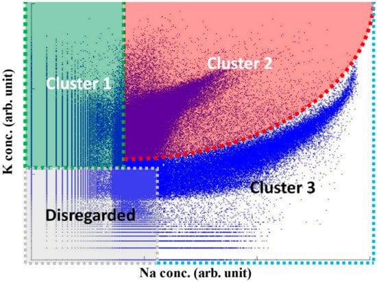
Figure 1.
Cluster boundaries in logarithmic scale, where the boundaries are defined based on clustering analysis of Na and K content of individual aerosol particles.
2.5. Air Mass Back-Trajectories
Backward 72 h trajectories ending 500 m above ground level in Gothenburg were calculated using the HYSPLIT4 model [46]. New trajectories were started every 6 h, giving a total of 376 trajectories for the entire measurement period. The trajectories were analyzed by cluster analysis using the built-in analysis module of the HYSPLIT program. The clustering process is an iterative process wherein each step, the two closest clusters (trajectories) are paired until all trajectories are collected in one cluster [46]. The change in total spatial variance is calculated for each clustering step, and a large change in spatial variance indicates that two relatively different clusters (trajectories) have been paired. Large changes in variance occurred in the formation of 5 and 10 clusters, which suggested that solutions with 6 and 11 clusters provided useful solutions in the clustering analysis. The results from the smaller six-cluster solution are used in the present study.
2.6. Chemical Transport Modelling
The EMEP MSC-W chemical transport model (CTM) [36,47,48] was used to track the influences of different emission sources that may contribute to the observed K and Na concentrations in Gothenburg. The model is used in many different applications and includes treatment of the most important gases for describing photochemical ozone formation and secondary production of aerosol particles from anthropogenic and biogenic sources [8,49,50,51,52]. Primary emissions of particles from anthropogenic sources, sea salt, and wind-blown dust are also included in the model. Emissions of alkali compounds are not explicitly included in the model (except Na from sea salt). In the present work, regional-scale simulations were performed with the EMEP MSC-W CTM using a model domain that covers all of Europe and large parts of the North Atlantic Ocean and the Arctic area.
The EMEP model results used in this study are mostly taken from the model simulations described by Bergström et al. [53]. The EMEP MSC-W model was run with a relatively coarse resolution; each grid point covered an area of about 50 km × 50 km, and the lowest model layer was ca. 90 m thick. This limits the ability to model the impact of local emission sources in detail as the emissions will be diluted over an area of ca 2500 km2. The model will thus underestimate impacts from point (and small area) sources near the measurement site. The anthropogenic model emissions were handled as in Genberg et al. [50]; primary carbonaceous aerosol emissions from residential combustion were taken from a recently prepared bottom-up emission inventory for this sector [8], accounting for the semi-volatile components of the emissions; other primary carbonaceous aerosol emissions are taken from the EUCAARI inventory [8]; other anthropogenic emissions were taken from the standard EMEP emission inventory [36,54]. Emissions from open biomass fires (both wildfires and agricultural burning) were taken from the Fire Inventory from NCAR version 1.0 (FINNv1) [55]. Natural emissions of biogenic volatile organic compounds from vegetation and sea salt from the oceans are calculated within the model [36].
The temporal distribution of the emissions is described in detail by Simpson et al. [36]; for small scale non-industrial combustion (SNAP—Selected Nomenclature for Air Pollution—sector 2; dominated by residential combustion), the day-to-day variation of the emissions are based on the heating degree day concept, which means that the emissions depend on the daily temperatures in the respective emission areas [36].
3. Results and Discussion
3.1. Overview of Measured K and Na Concentrations
Figure 2 shows an overview of the Na and K concentrations measured during the period from 16 February to 20 May 2007, together with meteorological, PM10, and NOx data [43]. The Na and K concentrations are typically in the range 1–50 ng m−3 and show large variability on the time scale of a few hours for both elements with peak concentrations above 100 ng m−3 for Na. The time series indicate that the two concentrations are correlated during some periods, but this is not generally true and the Na/K ratio usually varies in the range from 0.1 to 20. The alkali concentrations do not appear to show a general trend related to seasonal changes, and the reasons for the observed concentration variability are instead to be sought in the changes in atmospheric conditions and source strengths.
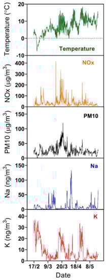
Figure 2.
Concentrations of Na and K in submicron particles as a function of time measured by the Alkali aerosol mass spectrometer (AMS), together with temperature, and particulate matter PM10, and NOx concentrations measured at the Femman station [43]. Displayed values are averages over 6 min intervals.
3.2. Influence of Local Meteorological Conditions
The meteorological conditions changed from winter to spring during the measurement period, and the monthly average temperatures were 0.5, 6.0, 9.1, and 12.0 °C during February, March, April, and May, respectively. The temperatures were close to the normal monthly averages for February and May, while March was 4 °C and April was 2 °C warmer than normal. Daily temperatures were below zero during several days in February, and peak day-time temperatures were in the range of 15 to 20 °C during some of the warmer periods. Ground-level temperature inversions are well known to have a strong influence on air quality in Gothenburg [56,57] and several strong inversions and associated periods of poor air quality occurred in March, while the effects of inversions on air quality were less important during other periods.
Figure 3 shows that the local wind speed has a relatively strong effect on the mean Na and K concentrations. Na concentrations increase considerably with wind speed above 3 m s−1, while the highest K concentrations are observed with wind speeds below 3 m s−1. Figure 4 illustrates that the wind direction also has an important effect on the concentrations of alkali-containing particles. High concentrations of Na-containing particles are observed with westerly winds from the nearby sea, while the highest K concentrations are observed for easterly winds from the inland region. Figure 5 shows that local temperature also has a substantial impact on the K concentrations. The concentrations of K (and Na) increase with decreasing temperature below 2 °C. The observed correlations between high Na concentrations and high wind speeds and westerly winds strongly indicate that the observed Na-rich particles mainly consist of sea salt particles. High K concentrations are, on the other hand, favored by low temperatures, low wind speeds, and winds from the inland, which suggests that they may originate from biomass burning in the nearby region during cold periods. It appears that the local meteorological conditions have an important impact on the concentrations of Na and K in PM1. However, the observed concentrations show large variations under similar meteorological conditions, which indicates that regional production of particles may not be sufficient to explain the observations.
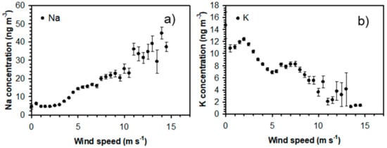
Figure 3.
(a) Na and (b) K concentrations as a function of wind speed for all data obtained during the measurement campaign. Error bars correspond to ±1 standard deviation.
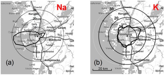
Figure 4.
(a) Na and (b) K concentrations as a function of wind direction (Femman station) for all data obtained during the measurement campaign.
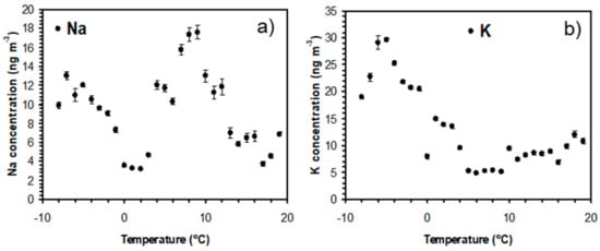
Figure 5.
(a) Na and (b) K concentrations as a function of temperature for all data obtained during the measurement campaign. Error bars correspond to ±1 standard deviation.
3.3. Influence of Air Mass History
To further evaluate the origin of the detected particles, back trajectories of air masses reaching Gothenburg were calculated and analyzed by group analysis. The results from a six-group solution are presented in Figure 6, where the traces for individual back trajectories are indicated. Figure 7 shows the resulting mean trajectories for the six group solutions and the relative contribution to each cluster in percent. Some of the clusters consist of trajectories with a complex pattern, while some were more directed from a certain region. The individual clusters are attributed to different regions of origin for the air masses: Central (C), Eastern (E), Northern (N), and Western Europe (W), as well as clusters with Atlantic (A) and Polar (P) origin.
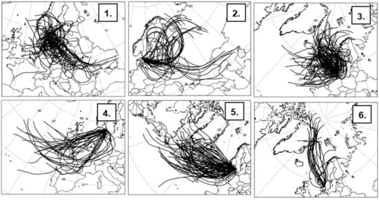
Figure 6.
Trajectory group analysis for six air mass types reaching Gothenburg during the period from 16 February 00:00 to 21 May 00:00 mean trajectories (uppermost panel), and individual trajectories attributed to the six groupings: (1)C, (2)E, (3)N, (4)W, (5)A, and (6)P. The traces correspond to 72 h backward trajectories calculated using the HYSPLIT4 model [46]. New trajectories were started every 6 h and ended 500 m above ground level in Gothenburg.
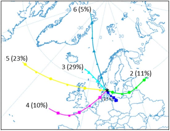
Figure 7.
Mean back trajectories based on the group analysis illustrated in Figure 6. The six groups and percent of the total number of trajectories assigned to each group are indicated. See text for further details.
Table 1 summarizes mean values for the alkali, PM10, and trace gas concentrations depending on the type of air mass reaching Gothenburg together with mean meteorological data. These data sets are only included from time periods where at least two consecutive air mass trajectories are attributed to the same group type. The highest mean Na concentration and the highest Na/K ratio are observed in air masses with an Atlantic origin (trajectory cluster No. 5). The highest mean K concentrations and lowest Na/K ratios are observed when the air masses have an Eastern or a Central European origin. In these cases, the observed Na/K ratios are consistent with alkali-containing particles originating from solid fuel combustion processes [32,33]. NO, NOx, and PM10 concentrations are also high for air mass types 1 and 2 compared with other types of air masses. The air masses originating from Northern and Western Europe, as well as from the Polar region, appear to consist of local polluted air with different degrees of marine character.

Table 1.
Back trajectory group analysis for six air mass types indicates the air mass category, number of 6 min samples, percent of the total number of trajectories assigned to each group, mean Na and K concentrations (ng m−3), Na/K concentration ratio, mean particulate matter (PM10) and trace gas concentrations (μg m−3), temperature (T) (°C), and wind speed (WS) (m s−1).
To further address the importance of regional emissions and long-range transport, the results from a short episode (March 24 to April 2, 2007) are illustrated in Figure 8 and Figure 9 [58]. The period is characterized by large daily variations in temperature and relatively strong night-time temperature inversions. Figure 8a shows that the air masses reaching Gothenburg during this period originated in Eastern Europe, while the air mass origin shifted before and after this period. In addition to solid fuel combustion, fires are common in Eastern Europe during this period of the year owing to agricultural burns and may potentially influence air quality in Northern Europe during short episodes. Figure 8b shows the distribution of fires in Europe (at 1 km resolution) during the short episode, where each dot on the map indicates a fire detected with the moderate resolution imaging spectroradiometer (MODIS) aboard the Terra satellite [59].
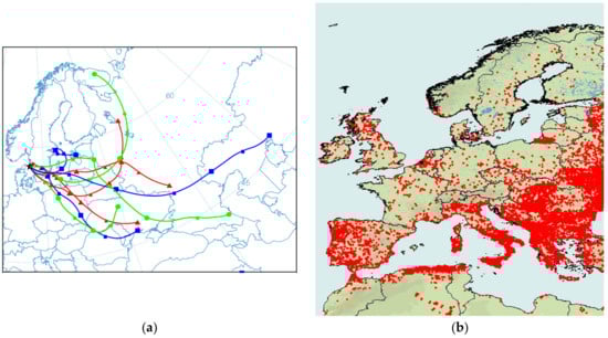
Figure 8.
(a) Seventy-two hour backward trajectories for 24 March to 1 April 2007. A new trajectory was started every 12 h. (b) Distribution of fires from the same period. Each dot on the map indicates a fire detected with the moderate resolution imaging spectroradiometer (MODIS) aboard the Terra satellite [58].
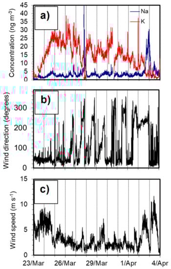
Figure 9.
Data from an episode from 24 March to 4 April; the vertical lines indicate midnight: (a) K and Na concentrations, (b) wind direction, and (c) wind speed.
Figure 9a shows a close up of the measured Na and K concentrations together with wind direction (Figure 9b) and wind speed (Figure 9c) data during the same period as covered in Figure 8. The K concentration was relatively high during this period, while Na was low during most of the period. An interesting effect was that both K and Na appear to follow a diurnal pattern during this particular period (24 Mar–1 Apr). The K concentrations often reached their highest values before noon, while Na peaked during the evening. The wind direction data (Figure 9b) indicate that the increase in Na concentration was related to a weak sea breeze that was observed daily in the afternoon and evening. The wind speed increased slightly during the sea breeze, but it was fairly low, and the Na signal may be attributed with limited formation of sea salt particles in the region near Gothenburg. The modulated K signal was likely the result of a combination of long-range transport and regional emissions from biomass burning that were trapped near the ground during the relatively cold nights with strong night-time temperature inversions.
The results in Figure 10 indicate that the concentrations of Na and K are generally correlated, in spite of occasional variations. Cluster 1 has a closer linkage in the winter season, while Cluster 2 has no apparent seasonal trend coupling. This agrees with the temperature dependence of K mass concentrations illustrated in Figure 11a, which shows that low temperatures favor Cluster 1, while Cluster 2 shows no clear dependence on temperature. They are both favored by low wind speeds (Figure 11b).
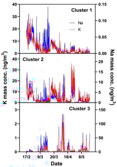
Figure 10.
Potassium (red lines) and sodium (blue) concentrations in Clusters 1 (upper panel), 2 (middle), and 3 (lower) during the measurement campaign.
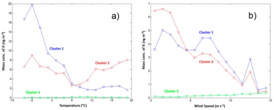
Figure 11.
K concentration in Clusters 1, 2, and 3 as a function of (a) temperature and (b) wind speed.
3.4. Comparison between Alkali-AMS and Chemical Transport Modeling Results
The experimental data are compared with results from model simulations with the EMEP MSC-W CTM, with a special emphasis on the influence of biomass burning and fossil fuel combustion. Figure 12 shows the measured total concentration of PM2.5 at the urban background station Femman and the modeled total concentration of carbonaceous PM from biomass burning (the sum of organic aerosol and elemental carbon from residential biomass combustion and open biomass fires). During the period 17 February–20 May 2007, the measured hourly PM2.5 concentration varies from 0 to about 50 µg m−3, and the highest concentrations occur during a handful of major peaks. The highest PM2.5 concentrations were observed during the period 23 March–2 April (two concentration peaks)—at the same time, the modeled concentration of particles from open fire and residential biomass burning is also high. There is a relatively high degree of correlation between the measured PM2.5 and the modeled biomass burning PM during the campaign period (r = 0.81, for hourly, moving 24 h mean concentrations; r = 0.72 for hourly concentrations). The modeled biomass combustion PM may constitute a considerable fraction of the total PM2.5 during some episodes. The average modeled biomass carbonaceous PM during the period is about 1.3 µg m−3, which is about 12% of the average measured PM2.5 concentration (11 µg m−3).
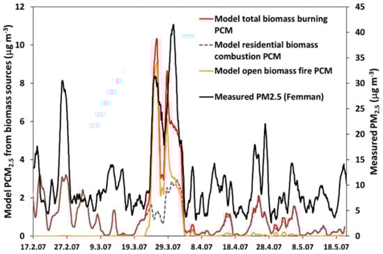
Figure 12.
PM2.5 concentrations at the urban background station Femman in Gothenburg (black line, right scale), during the period 17 Feb–20 May 2007 [43], and modeled concentrations of particulate carbonaceous matter (PCM) in PM2.5 from the following: residential biomass combustion (grey, dashed line), open biomass burning fires (including wild fires and agricultural fires, orange line), and total biomass burning PCM (red line). Unit: μg m−3. The data were smoothed using moving 24 h mean concentrations.
The measured K and particle number concentrations in the two combustion-related components (Clusters 1 and 2) are also compared to the results from the EMEP MSC-W model simulations. As K is not explicitly modeled, the comparison is based on model results for other particulate components that can be tracked to different source types. The model results for primary emitted fine particles (PPM2.5) from anthropogenic sources and open fires are used (Figure 13 and Figure 14). The modeled PPM2.5 is split into PPM2.5 from (i) residential biomass combustion, (ii) open vegetation fires (including both wildfires and agricultural burning), and (iii) other anthropogenic sources (predominantly fossil fuel sources).
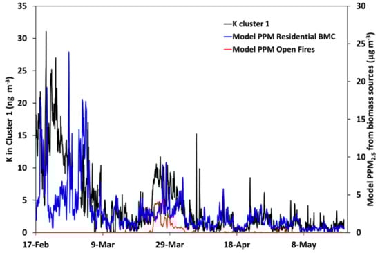
Figure 13.
Comparison of the modeled hourly concentrations of primary PM2.5 from residential biomass combustion (BMC, blue line) and open fires (red line) and measured (hourly average) concentrations of K in Cluster 1 (black line). Units, model results: ng m−3; measurements: ng K m−3.
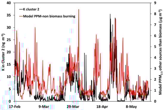
Figure 14.
Comparison of the modeled hourly concentrations of primary PM2.5 from fossil fuel combustion (red line) and measured (hourly average) concentrations of K in Cluster 2 (black line). Units, model results: µg m−3; measurements: ng K m−3.
Figure 13 shows a comparison between modeled concentrations of PPM2.5 from biomass combustion (residential + open fires) and the measured K concentration in Cluster 1. Overall, the modeled concentrations show a high degree of correlation with experimental data (see also Table 2; R = 0.64 for 24 h moving average concentrations) The main exception is a cold and windy six-day period in February, where the model produces significantly lower values (for the first five days). The meteorological conditions during this period result in a high demand for local residential heating, and we attribute this discrepancy to an underestimation of contributions from local sources—the total PM2.5 concentrations at the urban background station Femman were low during the first four days of the “Cluster 1 episode”, and this indicates that source(s) of the elevated K-concentrations measured with the AMS may have been located relatively close to the university site and possibly only impacting a relatively small area; the wind direction was rather stable during the whole episode. Local episodes of this type are difficult to model accurately with large scale chemical transport models owing to the low spatial resolution of the model simulations and emission data. The model simulations also confirm the importance of contributions from open fires, in particular, agricultural burns, in late March (compare with Figure 8 and Figure 9).
Table 2.
Correlation coefficients (r) between measured concentrations in Cluster 1 and 2 (particle number and K mass concentrations) and modeled mass concentrations of particulate matter from primary emissions (PPM) from selected sources.
Figure 14 illustrates the modeled concentration of PPM2.5 from fossil fuel combustion and the measured K concentration in Cluster 2. The correlation between the model and measurements is lower for Cluster 2 than for Cluster 1 (see also Table 2; R = 0.61 for 24 h moving average concentrations)—this is not surprising because the model PPM2.5 (from other sources than biomass burning) represents sums of many different sources, including, for example, traffic exhaust emissions, coal combustion, industrial processes, and waste burning. However, several features in the experimental data are qualitatively represented by the model results.
A separate set of model simulations were performed to investigate the correlation between the AMS measurements and individual primary particle emission categories. The correlation coefficients between measured concentrations and modeled PPM2.5 from different emission sources are given in Table 2. The measured concentrations in Cluster 1 are most strongly correlated with modeled biomass combustion particles, with a maximum r = 0.76 observed for total PPM2.5 from biomass combustion (residential combustion + open biomass burning). The correlation with modeled fossil fuel components is relatively low. In general, modeled concentrations are somewhat better correlated with measured number concentrations than with K concentrations. Although the measured Na concentrations are very low in Cluster 1, the correlation (not shown) between these and the modeled concentrations are as good as for K for most components. On the basis of the relatively high correlations observed, we conclude that the Cluster 1 particles observed with the Alkali-AMS are mainly emitted from biomass combustion.
The correlation coefficients between the measured concentrations in Cluster 2 and various model components are also given in Table 2. Cluster 2 corresponds less well to any modeled compound than Cluster 1 does; the highest correlations are found for emissions from the agricultural sector (SNAP-10; not including open burning of biomass, r = 0.65 when compared with the Cluster 2 number concentration) and for the sum of all “non-biomass” emission sources (r = 0.63). The correlation is especially low for particles from residential biomass combustion (r < 0.23). This indicates that Cluster 2 is at least not dominated by particles from residential biomass combustion in the region around Gothenburg. For Cluster 2, the correlation coefficients are similar for particle number and K concentrations, while they are lower for Na concentrations (not shown; r < 0.36 for all model components in Table 2 except for residential/non-industrial fossil fuel combustion, for which r = 0.61 for Na in Cluster 2). The lower correlations for Na have not been studied in detail, but one possible explanation may be interference from sea salt particles at the defined border between Cluster 2 and 3 (see Figure 1).
To investigate if emissions from any single geographical region could be responsible for a large fraction of the Cluster 2 particles, simplified model simulations, which track primary particle emissions from a number of areas in Europe (Sweden, Norway, Poland/Czechia/Slovakia (PCS), Eastern Europe (EEU = Russia, Belarus, the Baltic states, Finland, Ukraine) and Western Europe (WEU = Denmark, Germany, BeNeLux, France), the British Isles (United Kingdom, Ireland)), were performed with the EMEP MSC-W model. These simulations indicated that different Cluster 2 peaks correspond to different source regions; no single region seems to dominate Cluster 2 (see Figure S3). The highest measured concentrations in Cluster 2 (late April) seem to be associated with air masses from Western Europe. The broad peak at the end of March is associated with air from Eastern Europe and, for the later part, also with more southerly air that has passed Poland and other parts of Central Europe; Swedish emissions also influenced Gothenburg during this period. Several other peaks can be related to emissions in PCS, WEU, EEU, and Sweden.
We conclude that Cluster 2 seems to represent emissions from several different types of combustion sources and different source regions that contribute to air pollution in Gothenburg by long-range transport.
3.5. Comparison with Earlier Studies
The present results agree with measurements performed in Gothenburg during 2003 and 2004 with the Alkali-AMS that only monitored one type of alkali ion at the time [31]. Mass concentrations of alkali in ambient air varied in the range of 0.02–100 ng m−3 and the number of alkali-containing particles varied between 0.1 and 100 cm−3. The detected aerosol was concluded to be dominated by emissions from combustion of biomass and fossil fuels, with a significant contribution from sea-salt particles only during intrusion of marine air.
A long term measurement of Na and K in an urban and marine environment by Ooki et al. [59] reported an average K/Na ratio of 1.8 for the fine particles (D < 1.1 µm); the study concluded that the primary source of the fine particles was a domestic refuse incineration plant located within 15 km of the measurement site. This finding, K/Na ratio of 1.8, by Ooki et al. [59] agrees with the K/Na ratio of 1.2–1.7 reported by Mamane [60] from the direct household refuse incinerator aerosol measurements with the fine particles (D < 2.5 µm). In the present work, the air masses originating from Western Europe (W) had an average K/Na value of 2.2, which may suggest the emissions were associated with refuse combustions. A slightly higher value of K/Na than Mamane [60] can be explained by different combusted source materials. In European countries, the usage of both small and large scale biomass burning systems is common; especially during the cold winter period, usage of domestic heating systems with biomass fuel may contribute to the higher K/Na ratio.
Stohl et al. [61] reported measurements of Arctic air pollution owing to biomass burning associated with agricultural fire activities in Eastern Europe during the spring; this type of fire smoke can reach the Arctic region and potentially reduce the snow albedo and change the rate of snow/ice melting. The filter samples from the Zeppelin mountain station in Svalbard indicated elevated concentrations of levoglucosan, K, and CO for the biomass burning pollution events from 27 April to 9 May 2006. These results suggest that the monitoring of K and CO can be used as a good indicator for the potential contribution of air pollution from biomass burning in the Arctic region. As the SI-AMS has single-particle analysis capability, it has further potential to obtain more detailed information.
4. Conclusions
Aerosol mass spectrometry was used to measure the K and Na concentrations in submicron particles in Gothenburg, Sweden, during winter and spring seasons. Typical PM1 alkali concentrations were in the range from 1 to 50 ng m−3, but with large variations in concentrations and Na/K ratio depending on the prevailing conditions.
High concentrations of Na-containing particles were favored by westerly winds and high wind speeds. They were concluded to be related to sea salt particles in marine air masses. High concentrations of K-containing particles correlated with low temperatures and low wind speeds and were mainly associated with local and regional emissions and transport of air masses originating from continental Europe. Low Na/K ratios suggested that these particles originated from solid fuel combustion, including biomass burning.
During a spring-time PM episode, high K concentrations were observed. The K-rich particles were, to a large extent, transported from areas with extensive agricultural burns in Eastern Europe during the beginning of this period. During the later part, residential biomass combustion emissions also made significant contributions.
Further development and application of the methodology presented in this study, including analysis of single-particle data, may improve the ability to distinguish particles from different sources. To implement any regulatory approach to improve air quality, one needs to have a clear understanding of the emission sources. Alkali-AMS measurements can be a useful tool to identify contributions from biomass burning emissions to submicron particulate matter.
Supplementary Materials
The following are available online at https://www.mdpi.com/2073-4433/10/12/789/s1.
Author Contributions
Conceptualization, J.B.C.P.; methodology, R.B., X.K., and T.L.G.; software, X.K. and R.B.; validation, J.B.C.P.; formal analysis, J.B.C.P., R.B., X.K., and J.N.; investigation, J.N., T.L.G., M.S., and B.K.; resources, J.B.C.P.; data curation, J.N., T.L.G., J.B.C.P., and X.K.; writing—original draft preparation, J.B.C.P.; writing—review and editing, J.N., R.B., and X.K.; visualization, X.K., J.B.C.P., and R.B.; supervision, J.B.C.P.; project administration, J.B.C.P.; funding acquisition, J.B.C.P.
Funding
This work was supported by the Swedish Research Council for Environment, Agricultural Sciences, and Spatial Planning (Formas). Computer time for EMEP MSC-W model runs was supported by the Research Council of Norway through the NOTUR project EMEP (NN2890K) for the central processing unit (CPU) time, and NorStore project European Monitoring and Evaluation Programme (NS9005K) for storage of data. The research presented is a contribution to the Swedish strategic research area ‘ModElling the Regional and Global Earth system’ (MERGE).
Acknowledgments
The Environmental Office in Gothenburg is gratefully acknowledged for providing PM, trace gas, and meteorological data.
Conflicts of Interest
The authors declare no conflict of interest.
References
- Chen, J.; Li, C.; Ristovski, Z.; Milic, A.; Gu, Y.; Islam, M.S.; Wang, S.; Hao, J.; Zhang, H.; He, C.; et al. A review of biomass burning: Emissions and impacts on air quality, health and climate in China. Sci. Total Environ. 2017, 579, 1000–1034. [Google Scholar] [CrossRef] [PubMed]
- Kelly, F.J.; Fussell, J.C. Size, source and chemical composition as determinants of toxicity attributable to ambient particulate matter. Atmos. Environ. 2012, 60, 504–526. [Google Scholar] [CrossRef]
- Lee, A.; Kinney, P.; Chillrud, S.; Jack, D. A Systematic Review of Innate Immunomodulatory Effects of Household Air Pollution Secondary to the Burning of Biomass Fuels. Ann. Glob. Health 2015, 81, 368–374. [Google Scholar] [CrossRef]
- Deering-Rice, C.E.; Nguyen, N.; Lu, Z.; Cox, J.E.; Shapiro, D.; Romero, E.G.; Mitchell, V.K.; Burrell, K.L.; Veranth, J.M.; Reilly, C.A. Activation of TRPV3 by Wood Smoke Particles and Roles in Pneumotoxicity. Chem. Res. Toxicol. 2018, 31, 291–301. [Google Scholar] [CrossRef]
- Scott, A.F.; Reilly, C.A. Wood and Biomass Smoke: Addressing Human Health Risks and Exposures. Chem. Res. Toxicol. 2019, 32, 219–221. [Google Scholar] [CrossRef]
- Viana, M.; Kuhlbusch, T.A.J.; Querola, X.; Alastueya, A.; Harrison, R.M.; Hopke, P.K.; Winiwarter, W.; Vallius, M.; Szidat, S.; Prévôt, A.S.H.; et al. Source apportionment of particulate matter in Europe: A review of methods and results. Aerosol Sci. 2008, 39, 827–849. [Google Scholar] [CrossRef]
- Andersen, Z.J.; Wåhlin, P.; Raaschou-Nielsen, O.; Scheike, T.; Loft, S. Ambient particle source apportionment and daily hospital admissions among children and elderly in Copenhagen. J. Expo. Sci. Environ. Epidemiol. 2007, 17, 625–636. [Google Scholar] [CrossRef]
- Denier van der Gon, H.A.C.; Bergström, R.; Fountoukis, C.; Johansson, C.; Pandis, S.N.; Simpson, D.; Visschedijk, A.J.H. Particulate emissions from residential wood combustion in Europe–revised estimates and an evaluation. Atmos. Chem. Physics 2015, 15, 6503–6519. [Google Scholar] [CrossRef]
- Glasius, M.; Hansen, A.; Claeys, M.; Henzing, J.; Jedynska, A.; Kasper-Giebl, A.; Kistler, M.; Kristensen, K.; Martinsson, J.; Maenhaut, W. Composition and sources of carbonaceous aerosols in Northern Europe during winter. Atmos. Environ. 2018, 173, 127–141. [Google Scholar] [CrossRef]
- Szidat, S.; Jenk, T.M.; Synal, H.-A.; Kalberer, M.; Wacker, L.; Hajdas, I.; Kasper-Giebl, A.; Baltensperger, U. Contributions of fossil fuel, biomass burning, and biogenic emissions to carbonaceous aerosols in Zürich as traced by 14C. J. Geophys. Res. 2006, 111, D07206. [Google Scholar] [CrossRef]
- Szidat, S.; Prévôt, A.S.H.; Sandradewi, J.; Alfarra, M.R.; Synal, H-A.; Wacker, L.; Baltensperger, U. Dominant impact of residential wood burning on particulate matter in Alpine valleys during winter. Geophys. Res. Lett. 2007, 34, L05820. [Google Scholar] [CrossRef]
- Szidat, S.; Ruff, M.; Wacker, L.; Synal, H.A.; Hallquist, M.; Shannigrahi, A.S.; Yttri, K.E.; Dye, C.; Simpson, D. Fossil and non-fossil sources of organic carbon (OC) and elemental carbon (EC) in Göteborg, Sweden. Atmos. Chem. Phys. 2009, 9, 1521–1535. [Google Scholar] [CrossRef]
- Simoneit, B.R.T. Biomass Burning—A Review of Organic Tracers for Smoke from Incomplete Combustion. Appl. Geochem. 2002, 17, 129–162. [Google Scholar] [CrossRef]
- Elsasser, M.; Crippa, M.; Orasche, J.; DeCarlo, P.F.; Oster, M.; Pitz, M.; Cyrys, J.; Gustafson, T.L.; Pettersson, J.B.C.; Schnelle-Kreis, J.; et al. Organic molecular markers and signature from wood combustion particles in winter ambient aerosols: aerosol mass spectrometer (AMS) and high time-resolved GC-MS measurements in Augsburg, Germany. Atmos. Chem. Phys. 2012, 12, 6113–6128. [Google Scholar] [CrossRef]
- Tao, J.; Zhang, L.M.; Zhang, R.J.; Wu, Y.F.; Zhang, Z.S.; Zhang, X.L.; Tang, Y.X.; Cao, J.J.; Zhang, Y.H. Uncertainty Assessment of Source Attribution of PM2.5 and its Water-soluble Organic Carbon Content using Different Biomass Burning Tracers in Positive Matrix Factorization Analysis–A Case Study in Beijing, China. Sci. Total Environ. 2016, 543, 326–335. [Google Scholar] [CrossRef]
- Fourtziou, L.; Liakakou, E.; Stavroulas, I.; Theodosi, C.; Zarmpas, P.; Psiloglou, B.; Sciare, J.; Maggos, T.; Bairachtari, K.; Bougiatioti, A. Multi-tracer Approach to Characterize Domestic Wood Burning in Athens (Greece) during Wintertime. Atmos. Environ. 2017, 148, 89–101. [Google Scholar] [CrossRef]
- Nielsen, I.E.; Eriksson, A.C.; Lindgren, R.; Martinsson, J.; Nystrom, R.; Nordin, E.Z.; Sadiktsis, I.; Boman, C.; Nojgaard, J.K.; Pagels, J. Time-resolved Analysis of Particle Emissions from Residential Biomass Combustion Emissions of Refractory Black Carbon, PAHs and Organic Tracers. Atmos. Environ. 2017, 165, 179–190. [Google Scholar] [CrossRef]
- Achad, M.; Caumo, S.; Vasconcellos, P.D.; Bajano, H.; Gomez, D.; Smichowski, P. Chemical Markers of Biomass Burning: Determination of Levoglucosan, and Potassium in Size-classified Atmospheric Aerosols Collected in Buenos Aires, Argentina by Different Analytical Techniques. Microchem. J. 2018, 139, 181–187. [Google Scholar] [CrossRef]
- Rad, F.M.; Spinicci, S.; Silvergren, S.; Nilsson, U.; Westerholm, R. Validation of a HILIC/ESI-MS/MS Method for the Wood Burning Marker Levoglucosan and its Isomers in Airborne Particulate Matter. Chemosphere 2018, 211, 617–623. [Google Scholar]
- Elsasser, M.; Busch, C.; Orasche, J.; Schön, C.; Hartmann, H.; Schnelle-Kreis, J.; Zimmermann, R. Dynamic Changes of the Aerosol Composition and Concentration during Different Burning Phases of Wood Combustion. Energy Fuels 2013, 27, 4959–4968. [Google Scholar] [CrossRef]
- Pagels, J.; Dutcher, D.D.; Stolzenburg, M.R.; McMurry, P.H.; Galli, M.E.; Gross, D.S. Fine-particle emissions from solid biofuel combustion studied with single-particle mass spectrometry: Identification of markers for organics, soot, and ash components. J. Geophys. Res. Atmos. 2013, 118, 859–870. [Google Scholar] [CrossRef]
- Echalar, F.; Gaudichet, A.; Cachier, H.; Artaxo, P. Aerosol Emissions by Tropical Forest and Savanna Biomass Burning: Characteristic Trace-Elements and Fluxes. Geophys. Res. Lett. 1995, 22, 3039–3042. [Google Scholar] [CrossRef]
- Lee, T.; Sullivan, A.P.; Mack, L.; Jimenez, J.L.; Kreidenweis, S.M.; Onasch, T.B.; Worsnop, D.R.; Malm, W.; Wold, C.E.; Hao, W.M. Chemical Smoke Marker Emissions During Flaming and Smoldering Phases of Laboratory Open Burning of Wildland Fuels. Aerosol Sci. Tech. 2010, 44, I–V. [Google Scholar] [CrossRef]
- Suess, D.T.; Prather, K.A. Mass Spectrometry of Aerosols. Chem. Rev. 1999, 99, 3007. [Google Scholar] [CrossRef]
- Johnston, M.V. Sampling and Analysis of Individual Particles by Aerosol Mass Spectrometry. J. Mass. Spectrom. 2000, 35, 585–595. [Google Scholar] [CrossRef]
- Noble, C.A.; Prather, K.A. Real-time single particle mass spectrometry: A historical review of a quarter century of the chemical analysis of aerosols. Mass Spectrom. Rev. 2000, 19, 248–274. [Google Scholar] [CrossRef]
- Coe, H.; Allan, J.D.; Alfarra, M.R.; Bower, K.N.; Flynn, M.J.; McFiggans, G.B.; Topping, D.O.; Williams, P.I.; O’Dowd, C.D.; Dall’Osto, M. Chemical and physical characteristics of aerosol particles at a remote coastal location, Mace Head, Ireland, during NAMBLEX. Atmos. Chem. Phys. 2006, 6, 3289–3301. [Google Scholar] [CrossRef]
- Canagaratna, M.R.; Jayne, J.T.; Jimenez, J.L.; Allan, J.D.; Alfarra, M.R.; Zhang, Q.; Onasch, T.B.; Drewnick, F.; Coe, H.; Middlebrook, A. Chemical and microphysical characterization of ambient aerosols with the aerodyne aerosol mass spectrometer. Mass Spectrom. Rev. 2007, 26, 185–222. [Google Scholar] [CrossRef]
- Svane, M.; Hagström, M.; Pettersson, J.B.C. Chemical Analysis of Individual Alkali-Containing Aerosol Particles: Design and Performance of a Surface Ionization Particle Beam Mass Spectrometer. Aerosol Sci. Technol. 2004, 38, 655–663. [Google Scholar] [CrossRef]
- Svane, M.; Gustafsson, T.L.; Kovacevik, B.; Noda, J.; Andersson, P.U.; Nilsson, E.D.; Pettersson, J.B.C. On-line chemical analysis of individual alkali-containing aerosol particles by surface ionization combined with time-of-flight mass spectrometry. Aerosol Sci. Technol. 2009, 43, 453–661. [Google Scholar] [CrossRef]
- Svane, M.; Janhäll, S.; Hagström, M.; Hallquist, M.; Pettersson, J.B.C. On-line Alkali Analysis of Individual Aerosol Particles in Urban Air. Atmos. Environ. 2005, 39, 6919–6930. [Google Scholar] [CrossRef]
- Svane, M.; Hagström, M.; Pettersson, J.B.C. Online Measurements of Individual Alkali-Containing Particles Formed in Biomass and Coal Combustion: Demonstration of an Instrument Based on Surface Ionization Technique. Energy Fuels. 2005, 19, 411–417. [Google Scholar] [CrossRef]
- Svane, M.; Hagström, M.; Davidsson, K.O.; Boman, J.; Pettersson, J.B.C. Cesium as a Tracer for Alkali Processes in a Large-scale Combustion Facility. Energy Fuels 2006, 20, 979–985. [Google Scholar] [CrossRef]
- Hu, Q.H.; Xie, Z.Q.; Wang, X.M.; Kang, H.; Zhang, P. Levoglucosan indicates high levels of biomass burning aerosols over oceans from the Arctic to Antarctic. Sci. Rep. 2013, 3, 3119. [Google Scholar] [CrossRef] [PubMed]
- Pratap, V.; Chen, Y.; Yao, G.; Nakao, S. Temperature effects on multiphase reactions of organic molecular markers: A modeling study. Atmos. Environ. 2018, 179, 40–48. [Google Scholar] [CrossRef]
- Simpson, D.; Benedictow, A.; Berge, H.; Bergström, R.; Emberson, L.D.; Fagerli, H.; Flechard, C.R.; Hayman, G.D.; Gauss, M.; Jonson, J.E. The EMEP MSC-W chemical transport model–Technical description. Atmos. Chem. Phys. 2012, 12, 7825–7865. [Google Scholar] [CrossRef]
- Liu, P.; Ziemann, P.J.; Kittelson, D.B.; McMurry, P.H. Generating Particle Beams of Controlled Dimensions and Divergence: I. Theory of Particle Motion in Aerodynamic Lenses and Nozzle Expansions. Aerosol Sci. Technol. 1995, 22, 292–313. [Google Scholar] [CrossRef]
- Liu, P.; Ziemann, P.J.; Kittelson, D.B.; McMurry, P.H. Generating Particle Beams of Controlled Dimensions and Divergence: Ii. Experimental Evaluation of Particle Motion in Aerodynamic Lenses and Nozzle Expansions. Aerosol Sci. Technol. 1995, 22, 314–324. [Google Scholar] [CrossRef]
- Jayne, J.T.; Leard, D.C.; Zhang, X.; Davidovits, P.; Smith, K.A.; Kolb, C.A.; Worsnop, D.R. Development of an Aerosol Mass Spectrometer for Size and Composition Analysis of Submicron Particles. Aerosol Sci. Technol. 2000, 33, 49–70. [Google Scholar] [CrossRef]
- Jimenez, J.L.; Jayne, J.T.; Shi, Q.; Kolb, C.A.; Worsnop, D.R.; Yourshaw, I.; Seinfeld, J.H.; Flagan, R.C.; Zhang, X.; Smith, K.A. Ambient Aerosol Sampling Using the Aerodyne Aerosol Mass Spectrometer. J. Geophys. Res. 2003, 108, 8425. [Google Scholar] [CrossRef]
- Ionov, N.I. Progress in Surface Science. S G Davison, Pergamon Press: Oxford, UK, 1972; Volume 1. [Google Scholar]
- Zandberg, E.Y. Surface-Ionization Detection of Particles. Tech. Phys. 1995, 65, 1–38. [Google Scholar]
- The Environmental Management office of the City of Gothenburg (miljoforvaltningen@miljo.goteborg.se). Air quality monitoring data from the Femman site in Gothenburg (and most other Swedish air quality monitoring stations). Available online: https://shair.smhi.se/portal/concentrations-in-air (accessed on 1 December 2019).
- Ester, M.; Kriegel, H.; Sander, J.; Xu, X. A density-based algorithm for discovering clusters in large spatial databases with noise. In Proceedings of the Second International Conference on Knowledge Discovery and Data Mining, Portland, OR, USA, 2–4 August 1996; pp. 226–231. [Google Scholar]
- Daszykowski, M.; Walczak, B.; Massart, D.L. Looking for natural patterns in data. Part 1. Density-based approach. Chemom. Intell. Lab. Syst. 2001, 56, 83–92. [Google Scholar] [CrossRef]
- Draxler, R.R.; Hess, G.D. Description of the HYSPLIT4 Modeling System, NOAA Technical Memorandum ERL ARL-224; NOAA: Silver Spring, MD, USA, 2004. [Google Scholar]
- Bergström, R.; Denier van der Gon, H.A.C.; Prévôt, A.S.H.; Yttri, K.E.; Simpson, D. Modelling of organic aerosols over Europe (2002–2007) using a volatility basis set (VBS) framework: Application of different assumptions regarding the formation of secondary organic aerosol. Atmos. Chem. Phys. 2012, 12, 8499–8527. [Google Scholar] [CrossRef]
- Simpson, D.; Bergström, R.; Tsyro, S.; Wind, P. Updates to the EMEP/MSC-W Model, 2018–2019, Transboundary Particulate Matter, Photo-Oxidants, Acidifying and Eutrophying Components. EMEP Status Report 1/2019; The Norwegian Meteorological Institute: Oslo, Norway, 2018; pp. 145–155. Available online: www.emep.int (accessed on 2 December 2019).
- Aas, W.; Tsyro, S.; Bieber, E.; Bergström, R.; Ceburnis, D.; Ellermann, T.; Fagerli, H.; Frölich, M.; Gehrig, R.; Makkonen, U. Lessons learnt from the first EMEP intensive measurement periods. Atmos. Chem. Phys. 2012, 12, 8073–8094. [Google Scholar] [CrossRef]
- Genberg, J.; Denier van der Gon, H.A.C.; Simpson, D.; Swietlicki, E.; Areskoug, H.; Beddows, D.; Ceburnis, D.; Fiebig, M.; Hansson, H.C.; Harrison, R.M.; et al. Light-absorbing carbon in Europe–measurement and modelling, with a focus on residential wood combustion emissions. Atmos. Chem. Phys. 2013, 13, 8719–8738. [Google Scholar] [CrossRef]
- Jonson, J.E.; Simpson, D.; Fagerli, H.; Solberg, S. Can we explain the trends in European ozone levels? Atmos. Chem. Phys. 2006, 6, 51–66. [Google Scholar] [CrossRef]
- Yttri, K.E.; Simpson, D.; Bergström, R.; Kiss, G.; Szidat, S.; Ceburnis, D.; Eckhardt, S.; Hueglin, C.; Nøjgaard, J.K.; Perrino, C. The EMEP Intensive Measurement Period campaign, 2008–2009: Characterizing carbonaceous aerosol at nine rural sites in Europe. Atmos. Chem. Phys. 2019, 19, 4211–4233. [Google Scholar] [CrossRef]
- Bergström, R.; Hallquist, M.; Simpson, D.; Wildt, J.; Mentel, T.F. Biotic stress: a significant contributor to organic aerosol in Europe? Atmos. Chem. Phys. 2014, 14, 13643–13660. [Google Scholar] [CrossRef]
- Mareckova, K.; Wankmueller, R.; Anderl, M.; Poupa, S.; Wieser, M. Inventory Review 2009. Emission Data Reported Under the LRTAP Convention and NEC Directive. Stage 1 and 2 Review. Status of Gridded Data and LPS Data; EMEP/CEIP Technical Report 1/2009; Umweltbundesamt GmbH: Vienna, Austria, 2009. [Google Scholar]
- Wiedinmyer, C.; Akagi, S.K.; Yokelson, R.J.; Emmons, L.K.; Al-Saadi, J.A.; Orlando, J.J.; Soja, A.J. The Fire Inventory from NCAR (FINN): A high resolution global model to estimate the emissions from open burning. Geosci. Model Dev. 2011, 4, 625–641. [Google Scholar] [CrossRef]
- Janhäll, S.; Andersson, P.U.; Olofson, K.F.G.; Pettersson, J.B.C.; Hallquist, M. Evolution of the Urban Aerosol during Winter Temperature Inversion Episodes. Atmos. Environ. 2006, 28, 5355–5366. [Google Scholar] [CrossRef]
- Olofson, K.F.G.; Andersson, P.U.; Hallquist, M.; Ljungström, E.; Tang, L.; Chen, D.; Pettersson, J.B.C. Urban aerosol evolution and particle formation during wintertime temperature inversions. Atmos. Environ. 2008, 43, 340–346. [Google Scholar] [CrossRef]
- Roy, D.P.; Borak, J.S.; Devadiga, S.; Wolfe, R.E.; Zheng, M.; Descloitres, J. The MODIS Land product quality assessment approach. Remote Sens. Environ. 2002, 83, 62–76. [Google Scholar] [CrossRef]
- Ooki, A.; Uematsu, M.; Miura, K.; Nakae, S. Sources of sodium in atmospheric fine particles. Atmos. Environ. 2002, 36, 4367–4374. [Google Scholar] [CrossRef]
- Mamane, Y. Estimate of Municipal Refuse Incinerator Contribution to Philadelphia Aerosol. 1. Source Analysis. Atmos. Environ. 1988, 22, 2411–2418. [Google Scholar] [CrossRef]
- Stohl, A.; Berg, T.; Burkhart, J.F.; Fjaeraa, A.M.; Forster, C.; Herber, A.; Hov, O.; Lunder, C.; McMillan, W.W.; Oltmans, S. Arctic smoke—Record high air pollution levels in the European Arctic due to agricultural fires in Eastern Europe in spring 2006. Atmos. Chem. Phys. 2007, 7, 511–534. [Google Scholar] [CrossRef]
© 2019 by the authors. Licensee MDPI, Basel, Switzerland. This article is an open access article distributed under the terms and conditions of the Creative Commons Attribution (CC BY) license (http://creativecommons.org/licenses/by/4.0/).