Sodar Observation of the ABL Structure and Waves over the Black Sea Offshore Site

 , , , ,
  , and
, and 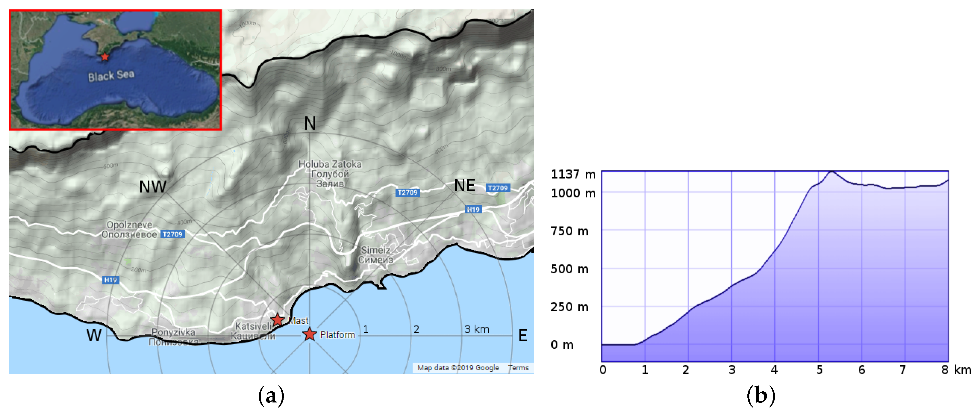
Abstract
:1. Introduction
2. Measurement Site and Equipment
3. Results
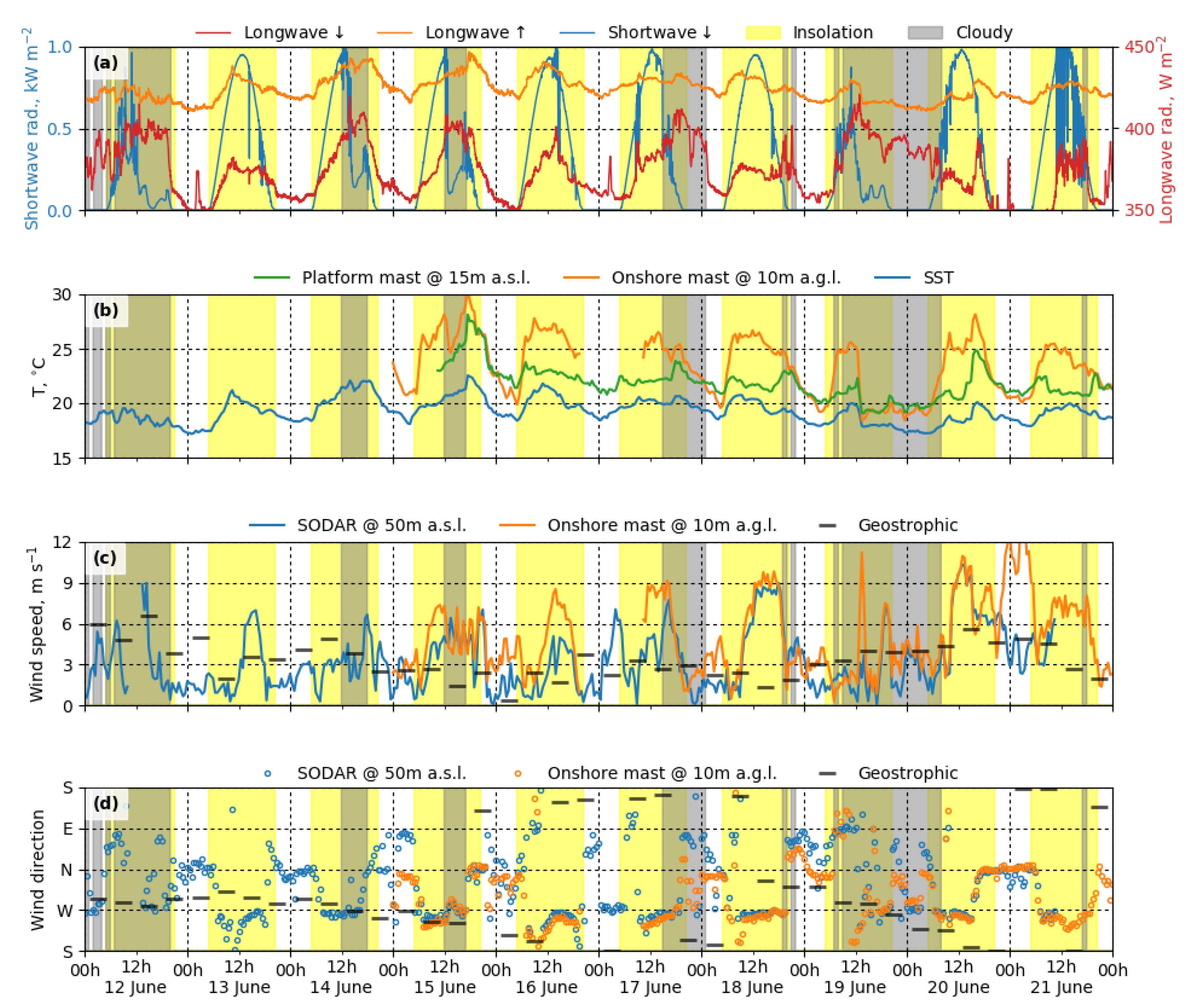
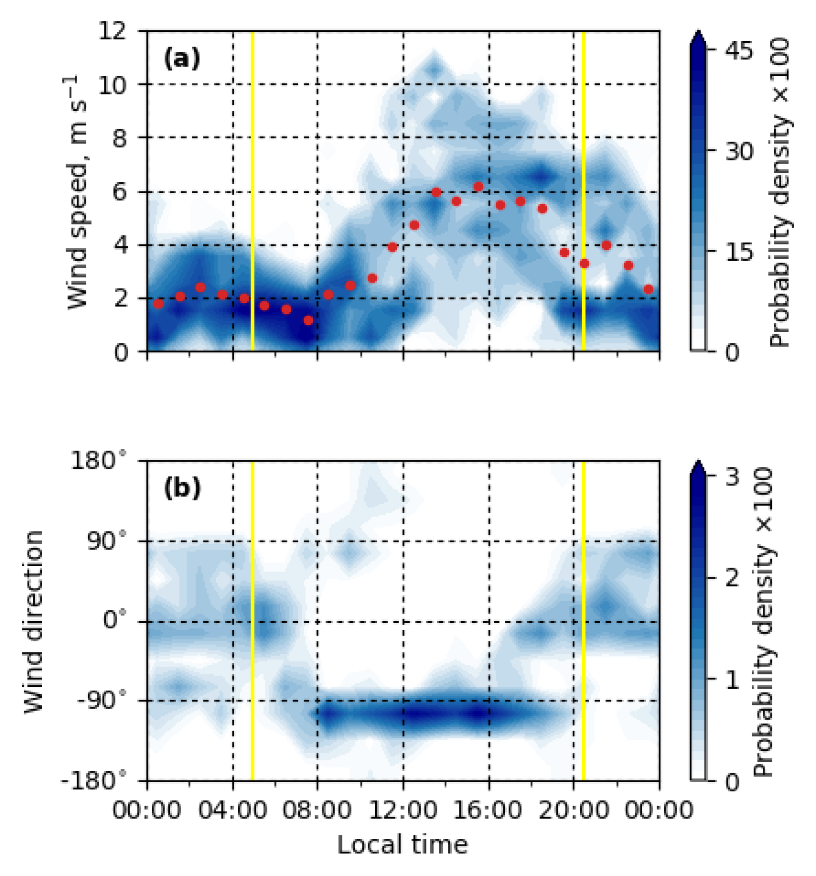
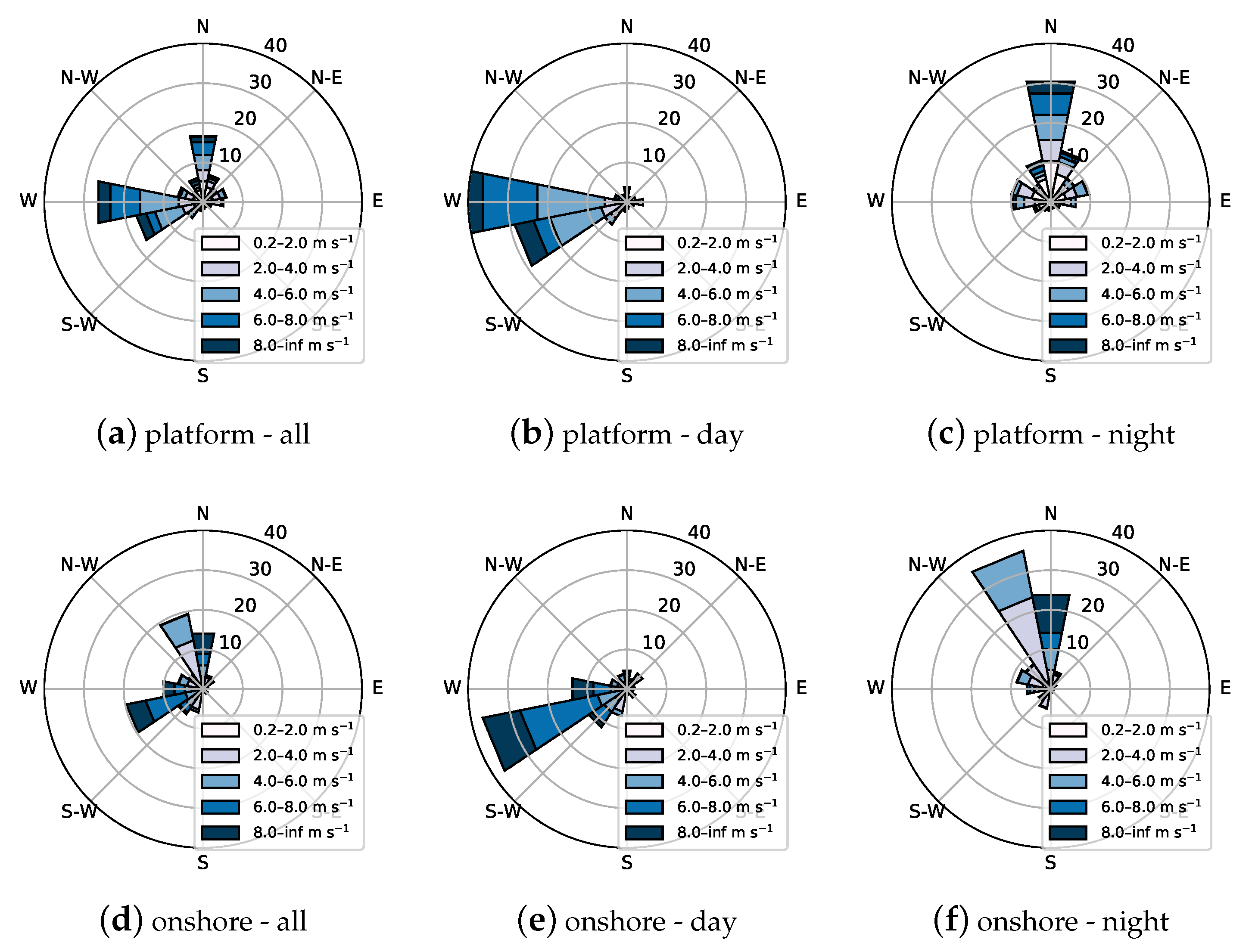
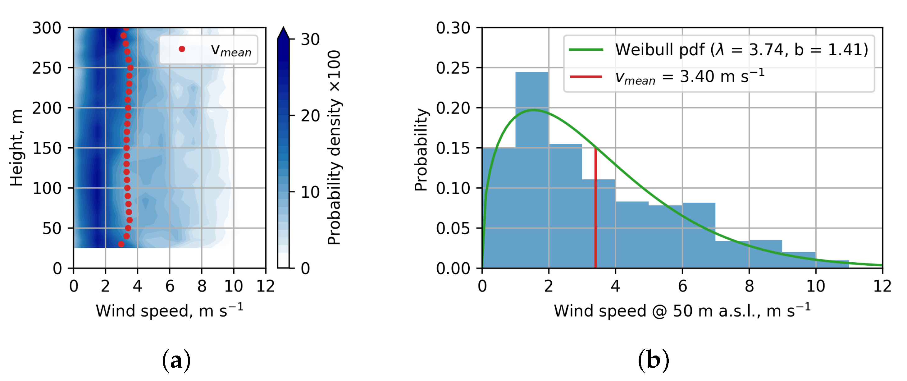
3.1. Diurnal Cycle of Meteorological Parameters
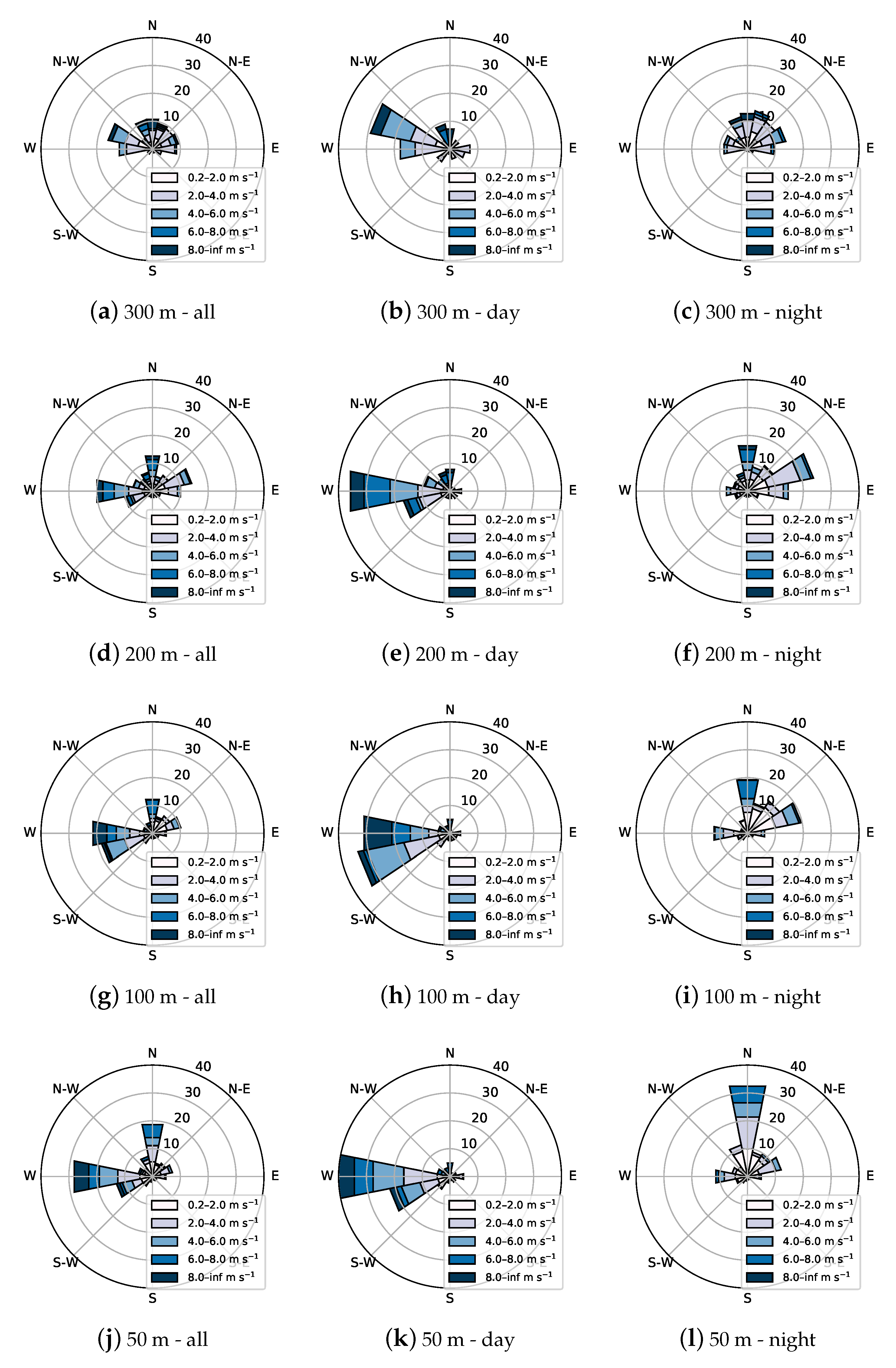
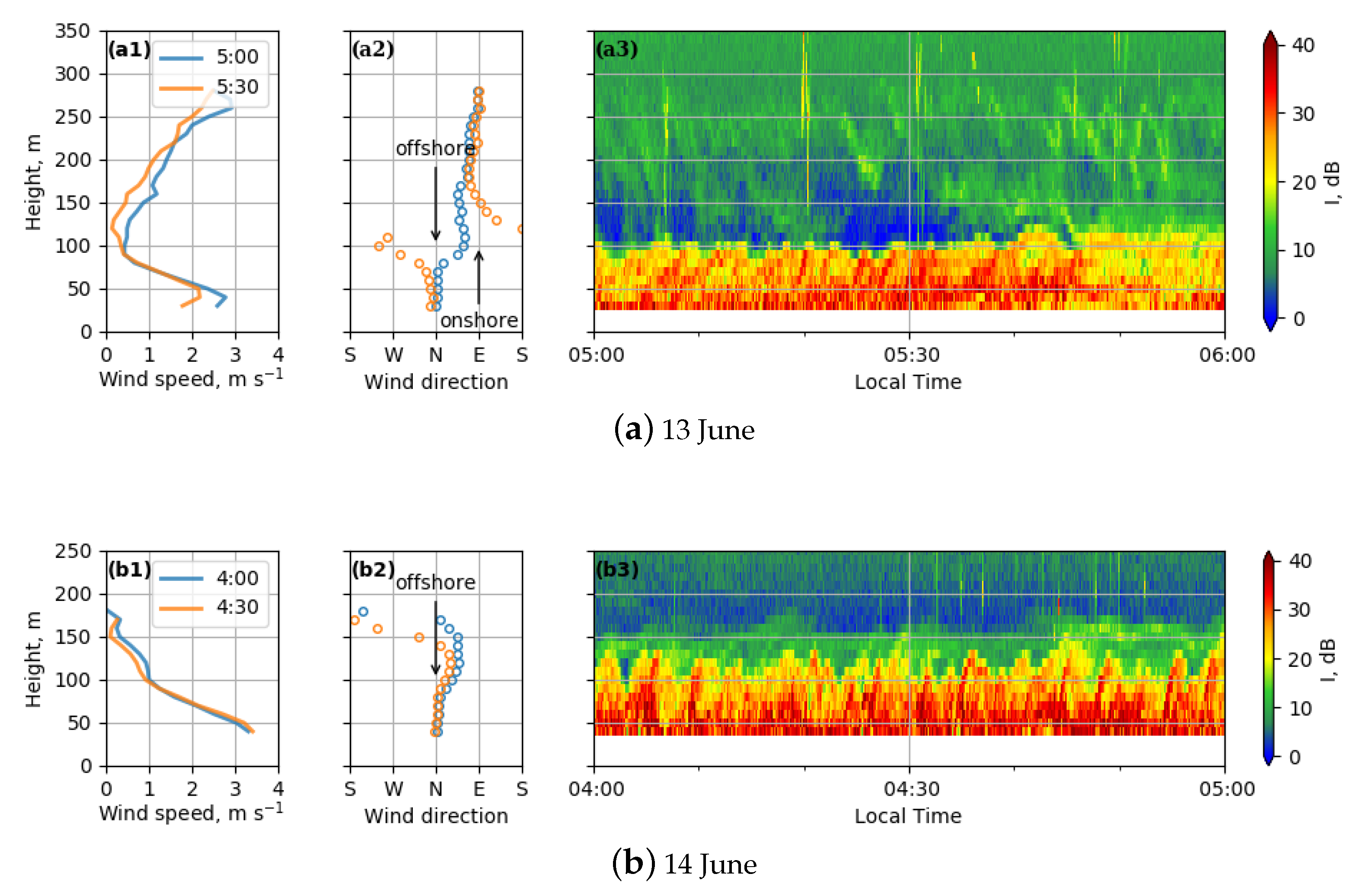
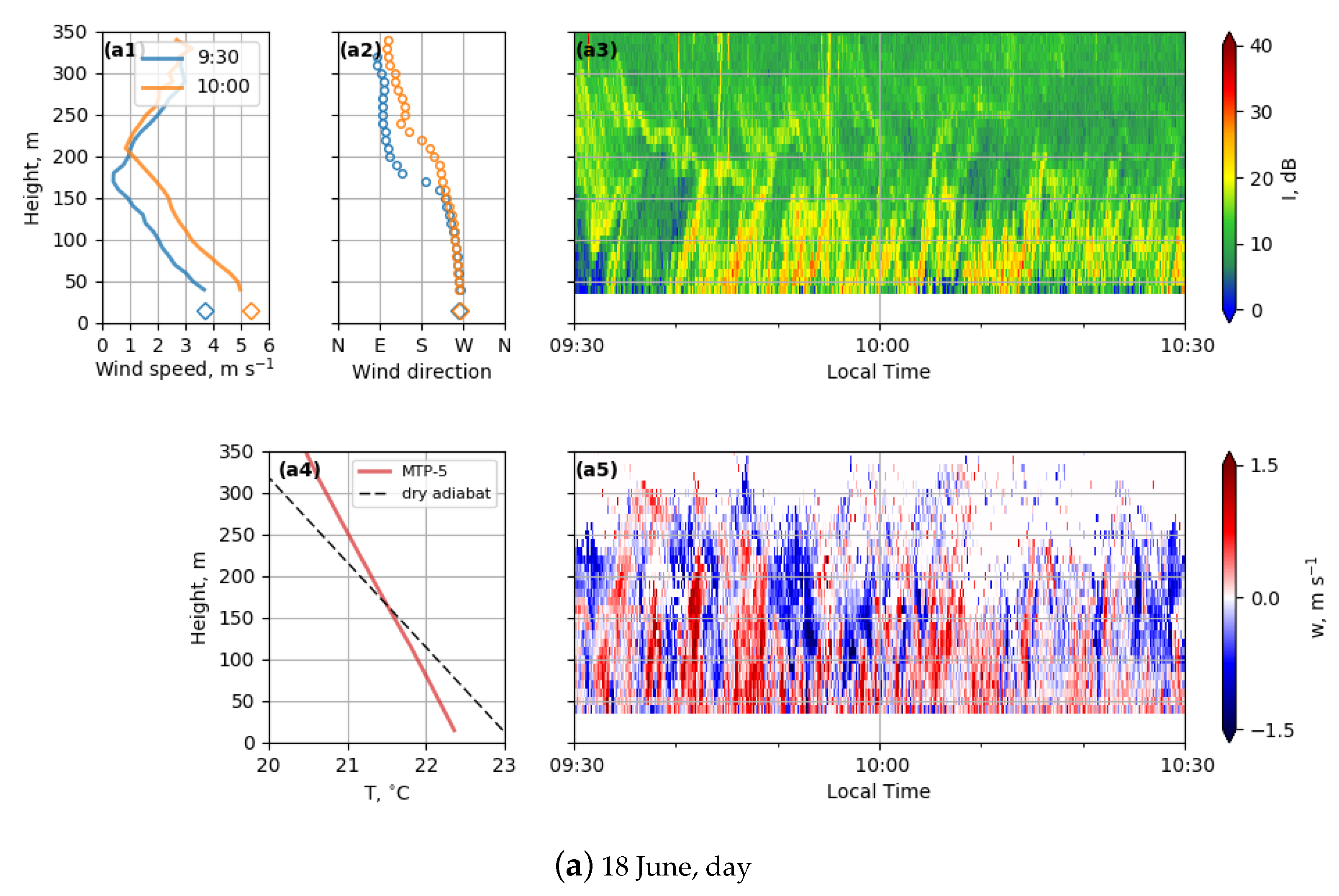
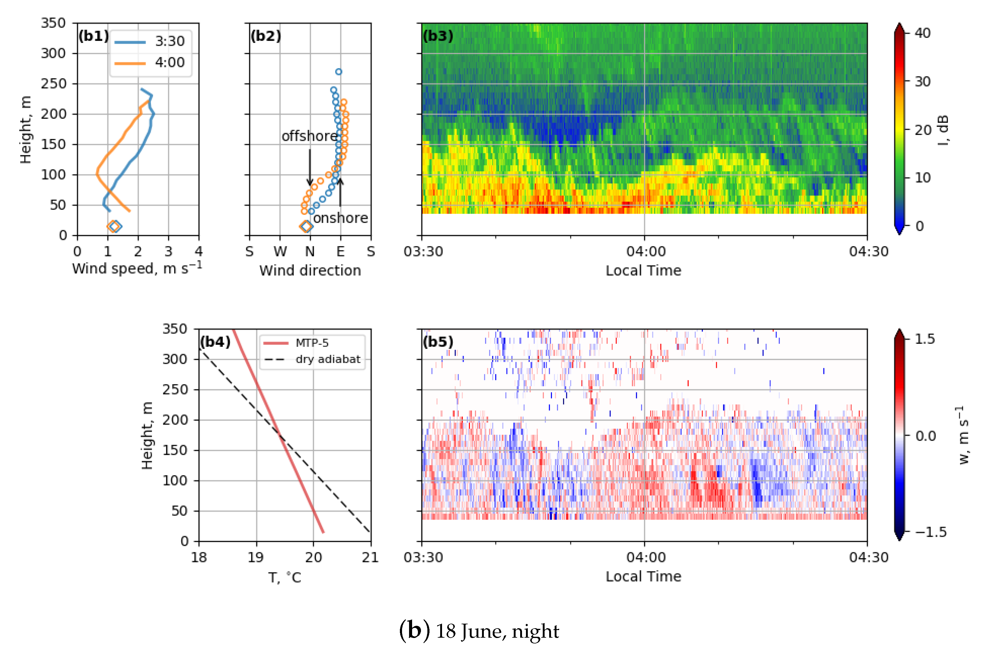
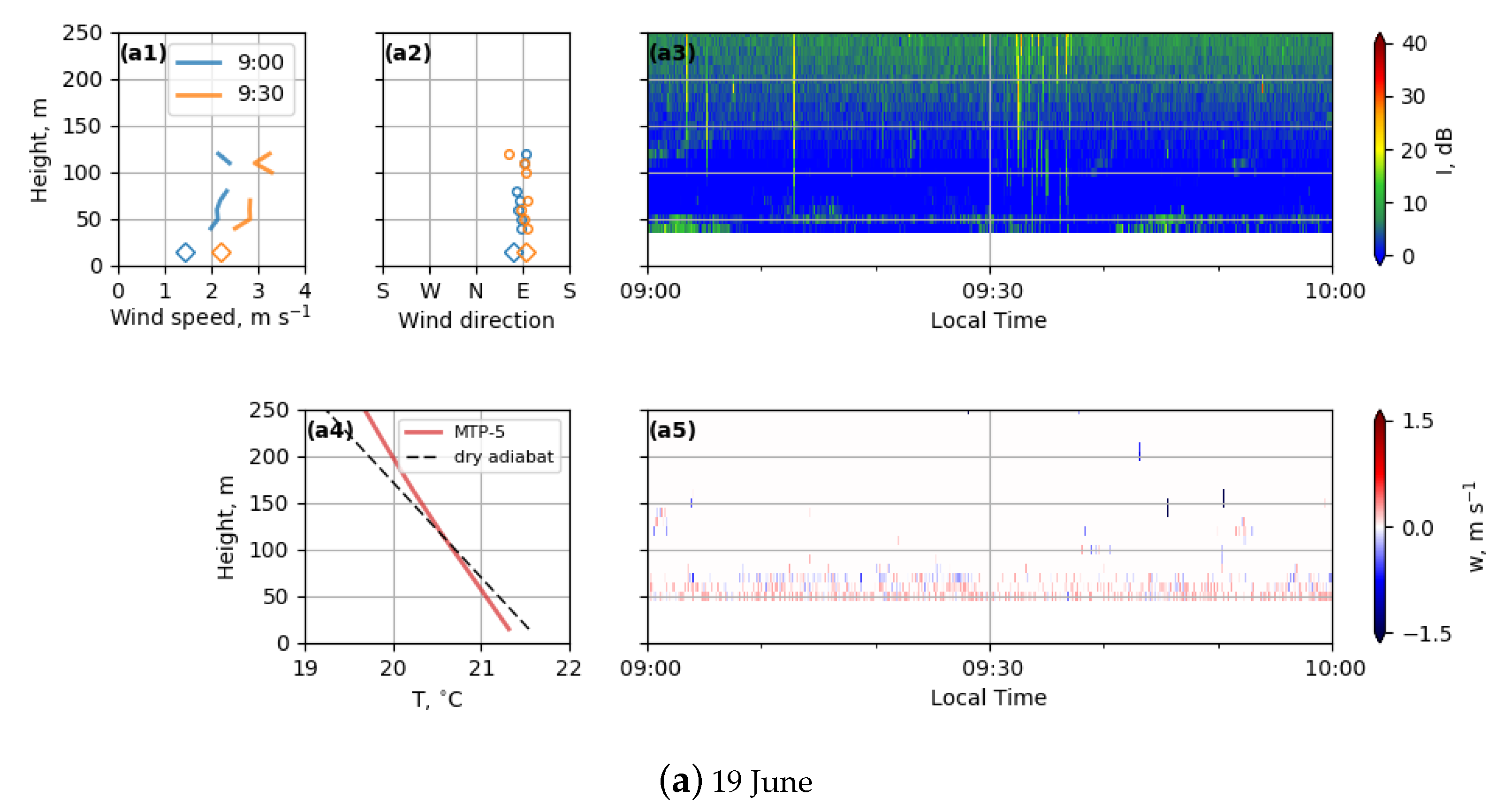
3.2. Vertical Structure of the Wind Field
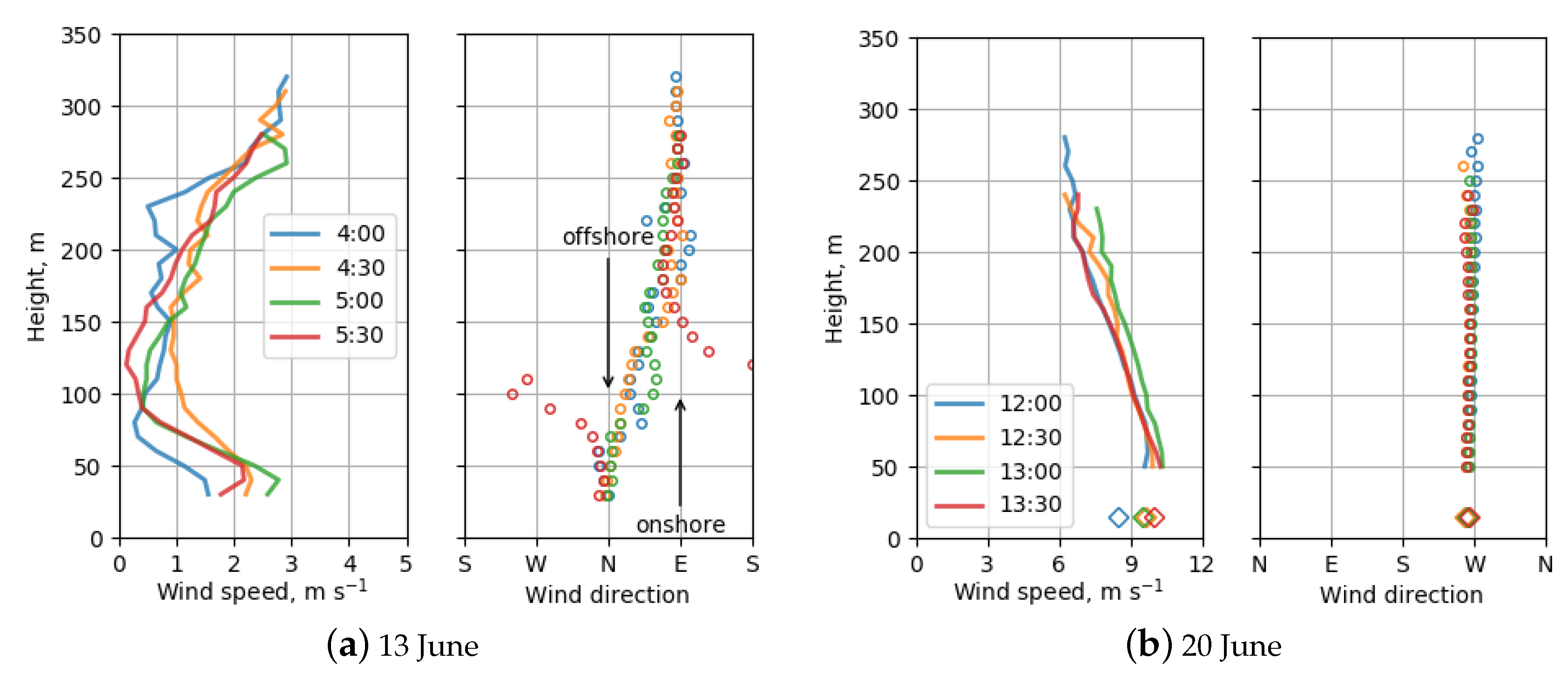
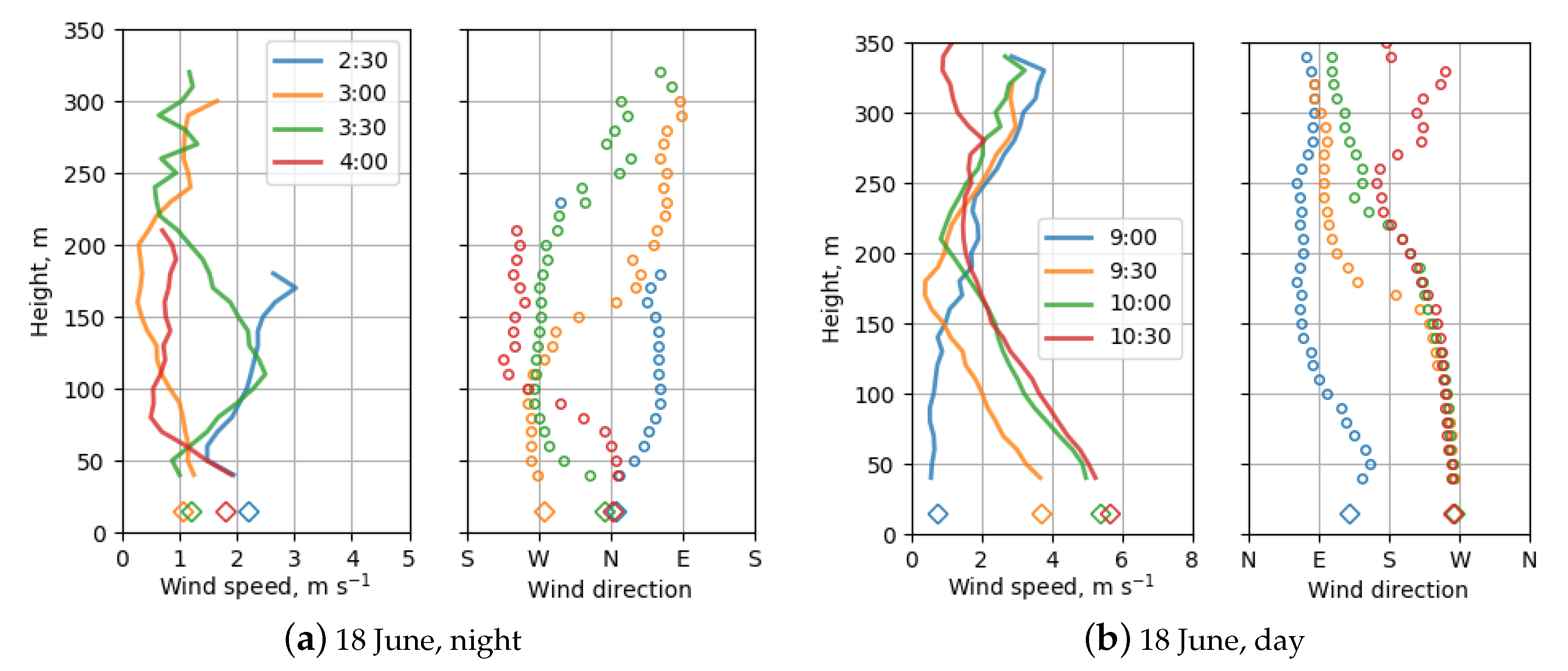
3.3. Observation of Wave Structures in Shear Flows
4. Discussion
5. Conclusions
Author Contributions
Funding
Acknowledgments
Conflicts of Interest
Abbreviations
| ABL | atmospheric boundary layer |
| a.s.l. | above sea level |
| a.g.l. | above ground level |
| KHB | Kelvin-Helmholtz billows |
| LLJ | low-level jet |
| SST | sea surface temperature |
References
- Crosman, E.T.; Horel, J.D. Sea and Lake Breezes: A Review of Numerical Studies. Bound.-Layer Meteorol. 2010, 137, 1–29. [Google Scholar] [CrossRef] [Green Version]
- Salvador, N.; Reis, N.C.; Santos, J.M.; Albuquerque, T.T.A.; Loriato, A.G.; Delbarre, H.; Augustin, P.; Sokolov, A.; Moreira, D.M. Evaluation of weather research and forecasting model parameterizations under sea-breeze conditions in a North Sea coastal environment. J. Meteorol. Res. 2016, 30, 998–1018. [Google Scholar] [CrossRef]
- Huang, Q.; Cai, X.; Song, Y.; Kang, L. A numerical study of sea breeze and spatiotemporal variation in the coastal atmospheric boundary layer at Hainan Island, China. Bound.-Layer Meteorol. 2016, 161, 543–560. [Google Scholar] [CrossRef]
- Olsen, B.T.; Hahmann, A.N.; Sempreviva, A.M.; Badger, J.; Jørgensen, H.E. An intercomparison of mesoscale models at simple sites for wind energy applications. Wind Energy Sci. 2017, 2, 211–228. [Google Scholar] [CrossRef] [Green Version]
- Salvação, N.; Soares, C.G. Wind resource assessment offshore the Atlantic Iberian coast with the WRF model. Energy 2018, 145, 276–287. [Google Scholar] [CrossRef]
- Banta, R.B.; Pichugina, Y.L.; Brewer, W.A.; James, E.P.; Olson, J.B.; Benjamin, S.G.; Carley, J.R.; Bianco, L.; Djalalova, I.V.; Wilczak, J.M.; et al. Evaluating and Improving NWP Forecast Models for the Future: How the Needs of Offshore Wind Energy Can Point the Way. Bull. Am. Meteorol. Soc. 2018, 99, 1155–1176. [Google Scholar] [CrossRef]
- Prósper, M.A.; Otero-Casal, C.; Fernández, F.C.; Miguez-Macho, G. Wind power forecasting for a real onshore wind farm on complex terrain using WRF high resolution simulations. Renew. Energy 2019, 135, 674–686. [Google Scholar] [CrossRef]
- Archer, C.L.; Colle, B.A.; Delle Monache, L.; Dvorak, M.J.; Lundquist, J.; Bailey, B.H.; Beaucage, P.; Churchfield, M.J.; Fitch, A.C.; Kosovic, B.; et al. Meteorology for coastal/offshore wind energy in the United States: Recommendations and research needs for the next 10 years. Bull. Am. Meteorol. Soc. 2014, 95, 515–519. [Google Scholar] [CrossRef]
- Valldecabres, L.; Nygaard, N.; Vera-Tudela, L.; von Bremen, L.; Kühn, M. On the Use of Dual-Doppler Radar Measurements for Very Short-Term Wind Power Forecasts. Remote Sens. 2018, 10, 1701. [Google Scholar] [CrossRef] [Green Version]
- Rakesh, P.; Sandeepan, B.S.; Venkatesan, R.; Baskaran, R. Observation and numerical simulation of submesoscale motions within sea breeze over a tropical coastal site: A case study. Atmos. Res. 2017, 198, 205–215. [Google Scholar] [CrossRef]
- Svensson, N.; Arnqvist, J.; Bergström, H.; Rutgersson, A.; Sahlée, E. Measurements and Modelling of Offshore Wind Profiles in a Semi-Enclosed Sea. Atmosphere 2019, 10, 194. [Google Scholar] [CrossRef] [Green Version]
- Lundquist, J.K.; Wilczak, J.M.; Ashton, R.; Bianco, L.; Brewer, W.A.; Choukulkar, A.; Clifton, A.; Debnath, M.; Delgado, R.; Friedrich, K.; et al. Assessing state-of-the-art capabilities for probing the atmospheric boundary layer: The XPIA field campaign. Bull. Am. Meteorol. Soc. 2017, 98, 289–314. [Google Scholar] [CrossRef]
- Kallistratova, M.; Coulter, R. Application of sodars in the study and monitoring of the environment. Meteorol. Atmos. Phys. 2004, 85, 21–37. [Google Scholar] [CrossRef]
- Lyulyukin, V.S.; Kallistratova, M.A.; Kouznetsov, R.D.; Kuznetsov, D.D.; Chunchuzov, I.P.; Chirokova, G.Y. Internal Gravity-Shear Waves in the Atmospheric Boundary Layer by the Acoustic Remote Sensing Data. Izv. Atmos. Ocean. Phys. 2015, 51, 193–202. [Google Scholar] [CrossRef]
- Kallistratova, M.A.; Lyulyukin, V.S.; Kouznetsov, R.D.; Petenko, I.V.; Zaitseva, D.V.; Kuznetsov, D.D. Sodars Studies of Kelvin-Helmholtz Billows in the Low-Level Jets. In Dynamics of Wave and Exchange Processes in the Atmosphere; Chketiani, O., Gorbunov, M., Kulichkov, S., Repina, I., Eds.; GEOS: Moscow, Russia, 2017; pp. 212–259. [Google Scholar]
- Zaitseva, D.V.; Kallistratova, M.A.; Lyulyukin, V.S.; Kouznetsov, R.D.; Kuznetsov, D.D. The Effect of Internal Gravity Waves on Fluctuations in Meteorological Parameters of the Atmospheric Boundary Layer. Izv. Atmos. Ocean. Phys. 2018, 54, 173–181. [Google Scholar] [CrossRef]
- Kallistratova, M.A.; Petenko, I.V.; Kouznetsov, R.D.; Kulichkov, S.N.; Chkhetiani, O.G.; Chunchusov, I.P.; Lyulyukin, V.S.; Zaitseva, D.V.; Vazaeva, N.V.; Kuznetsov, D.D.; et al. Sodar Sounding of the Atmospheric Boundary Layer: Review of Studies at the Obukhov Institute of Atmospheric Physics, Russian Academy of Sciences. Izv. Atmos. Ocean. Phys. 2018, 54, 242–256. [Google Scholar] [CrossRef]
- Petenko, I.; Argentini, S.; Casasanta, C.; Kallistratova, M.; Sozzi, R.; Viola, A. Wavelike Structures in the Turbulent Layer During the Morning Development of Convection at Dome C, Antarctica. Bound.-Layer Meteorol. 2016, 161, 289–307. [Google Scholar] [CrossRef] [Green Version]
- Petenko, I.; Argentini, S.; Casasanta, C.; Genthon, C.; Kallistratova, M. Stable Surface-Based Turbulent Layer During the Polar Winter at Dome C, Antarctica: Sodar and In Situ Observations. Bound.-Layer Meteorol. 2019, 171, 101–128. [Google Scholar] [CrossRef]
- Mastrantonio, G.; Petenko, I.; Viola, A.P.; Argentini, S.; Coniglio, L.; Monti, P.; Leuzzi, G. Influence of the synoptic circulation on the local wind field in a coastal area of the Tyrrhenian Sea. IOP Conf. Ser. Earth Environ. Sci. 2008, 1. [Google Scholar] [CrossRef]
- Federico, S.; Pasqualoni, L.; DeLeo, L.; Bellecci, C. A study of the breeze circulation during summer and fall 2008 in Calabria Italy. Atmos. Res. 2010, 97, 1–13. [Google Scholar] [CrossRef]
- Helmis, C.G.; Wang, Q.; Sgouros, G.; Wang, S.; Halios, C. Investigating the summertime low-level jet over the East Coast of the USA: A case study. Bound.-Layer Meteorol. 2013, 149, 259–276. [Google Scholar] [CrossRef]
- Calmet, I.; Mestayer, P.G. Study of the thermal internal boundary layer during sea-breeze events in the complex coastal area of Marseille. Theor. Appl. Climatol. 2016, 123, 801–826. [Google Scholar] [CrossRef]
- Barantiev, D.; Batchvarova, E.; Novitsky, M. Breeze circulation classification in the coastal zone of the town of Ahtopol based on data from ground based acoustic sounding and ultrasonic anemometer. Bulg. J. Meteorol. Hydrol. 2017, 22, 2–25. [Google Scholar]
- Chiba, O. Variability of the sea-breeze front from SODAR measurements. Bound.-Layer Meteorol. 1997, 82, 165–174. [Google Scholar] [CrossRef]
- Miller, S.T.K.; Keim, B.D.; Talbot, R.W.; Mao, H. Sea breeze: Structure, forecasting, and impacts. Rev. Geophys. 2003, 41. [Google Scholar] [CrossRef] [Green Version]
- Sha, W.; Ogawa, S.; Iwasaki, T.; Wang, Z. A Numerical Study on the Nocturnal Frontogenesis of the Sea-breeze Front. J. Meteorol. Soc. Jpn. 2004, 82, 817–823. [Google Scholar] [CrossRef] [Green Version]
- Plant, R.S.; Keith, G.J. Occurrence of Kelvin-Helmholtz Billows in Sea-breeze Circulations. Bound.-Layer Meteorol. 2007, 122, 1–15. [Google Scholar] [CrossRef] [Green Version]
- Feliks, Y.; Tziperman, E.; Farrell, B. Non-normal growth of Kelvin-Helmholtz eddies in a sea breeze. Q. J. R. Meteorol. Soc. 2014, 140, 2147–2157. [Google Scholar] [CrossRef]
- Simpson, J.E.; Mansfield, D.A.; Milford, J.R. Inland penetration of sea-breeze fronts. Q. J. R. Meteorol. Soc. 1977, 103, 47–76. [Google Scholar] [CrossRef]
- Smith, R.B. Gravity wave effects on wind farm efficiency. Wind Energy 2010, 13, 449–458. [Google Scholar] [CrossRef]
- Ollier, S.J.; Watson, S.J.; Montavon, C. Atmospheric gravity wave impacts on an offshore wind farm. J. Phys. Conf. Ser. 2018, 1037, 072050. [Google Scholar] [CrossRef] [Green Version]
- Pospelov, M.; Biasio, F.D.; Goryachkin, Y.; Komarova, N.; Kuzmin, A.; Pampaloni, P.; Repina, I.; Sadovsky, I.; Zecchetto, S. Air–sea interaction in a coastal zone: The results of the CAPMOS’05 experiment on an oceanographic platform in the Black Sea. Atmos. Res. 2009, 94, 61–73. [Google Scholar] [CrossRef]
- Barantiev, D.; Novitsky, M.; Batchvarova, E. Meteorological observations of the coastal boundary layer structure at the Bulgarian Black Sea coast, Adv. Sci. Res. 2011, 6, 251–259. [Google Scholar] [CrossRef] [Green Version]
- Efimov, V.V.; Krupin, A.V. Breeze Circulation in the Black Sea Region. Russ. Meteorol. Hydrol. 2016, 41, 240–246. [Google Scholar] [CrossRef]
- Davy, R.; Gnatiuk, N.; Pettersson, L.; Bobylev, L. Climate change impacts on wind energy potential in the European domain with a focus on the Black Sea. Renew. Sustain. Energy Rev. 2018, 2018, 1652–1659. [Google Scholar] [CrossRef] [Green Version]
- Rusu, E.A. 30-year projection of the future wind energy resources in the coastal environment of the Black Sea. Renew. Energy 2019, 139, 228–234. [Google Scholar] [CrossRef]
- Kouznetsov, R.D. LATAN-3 sodar for investigation of the atmospheric boundary layer. Atmos. Ocean. Opt. 2007, 20, 749–753. [Google Scholar]
- Kouznetsov, R.D. The multi-frequency sodar with high temporal resolution. Meteorol. Z. 2009, 18, 169–173. [Google Scholar] [CrossRef]
- Kouznetsov, R. The new PC-based sodar LATAN-3. In Proceedings of the 13th International Symposium on Advancement of Boundary Layer Remote Sensing (ISARS-2006), Garmisch-Partenkirchen, Germany, 18–20 July 2006; pp. 18–20. [Google Scholar]
- Kadygrov, E.N.; Shur, G.N.; Viazankin, A.S. Investigation of atmospheric boundary layer temperature, turbulence, and wind parameters on the basis of passive microwave remote sensing. Radio Sci. 2003, 38. [Google Scholar] [CrossRef] [Green Version]
- Marty, C.; Philipona, R. The clear-sky index to separate clear-sky from cloudy-sky situations in climate research. Geophys. Res. Lett. 2000, 27, 2649–2652. [Google Scholar] [CrossRef]
- Mestayer, P.G.; Calmet, I.; Herlédant, O.; Barré, S.; Piquet, T.; Rosant, J.M. A coastal bay summer breeze study, part 1: Results of the Quiberon 2006 experimental campaign. Bound.-Layer Meteorol. 2018, 167, 1–26. [Google Scholar] [CrossRef]
- Tatarskii, V.I. The Effects of the Turbulent Atmosphere on Wave Propagation; Israel Program for Scientific Translations: Jerusalem, Israel, 1971. [Google Scholar]
- Muschinski, A. Possible effect of Kelvin-Helmholtz instability on VHF radar observation of the mean vertical wind. J. Appl. Meteorol. 1996, 35, 2210–2217. [Google Scholar] [CrossRef] [Green Version]
- Sun, J.; Mahrt, L.; Nappo, C.; Lenschow, D.H. Wind and temperature oscillations generated by wave-turbulence interactions in the stably stratified boundary layer. J. Atmos. Sci. 2015, 72, 1484–1503. [Google Scholar] [CrossRef]
- Adams, E. Four ways to win the sea breeze game. Sail. World 1997, 3, 44. [Google Scholar]
- Repina, I.; Artamonov, A.; Varentsov, M.; Kozyrev, A. Experimental Study of High Wind Sea Surface Drag Coefficient. Phys. Oceanogr. 2015, 1. [Google Scholar] [CrossRef] [Green Version]
- Lyulyukin, V.; Kouznetsov, R.; Kallistratova, M. The Composite Shape and Structure of Braid Patterns in Kelvin–Helmholtz Billows Observed with a Sodar. J. Atmos. Ocean. Technol. 2013, 30, 2704–2711. [Google Scholar] [CrossRef]
- Petenko, I.; Casasanta, G.; Bucci, S.; Kallistratova, M.; Sozzi, R.; Argentini, S. Turbulence, Low-Level Jets, and Waves in the Tyrrhenian Coastal Zone as Shown by Sodar. Atmosphere. in press.


© 2019 by the authors. Licensee MDPI, Basel, Switzerland. This article is an open access article distributed under the terms and conditions of the Creative Commons Attribution (CC BY) license (http://creativecommons.org/licenses/by/4.0/).
Share and Cite
Lyulyukin, V.; Kallistratova, M.; Zaitseva, D.; Kuznetsov, D.; Artamonov, A.; Repina, I.; Petenko, I.; Kouznetsov, R.; Pashkin, A. Sodar Observation of the ABL Structure and Waves over the Black Sea Offshore Site. Atmosphere 2019, 10, 811. https://doi.org/10.3390/atmos10120811
Lyulyukin V, Kallistratova M, Zaitseva D, Kuznetsov D, Artamonov A, Repina I, Petenko I, Kouznetsov R, Pashkin A. Sodar Observation of the ABL Structure and Waves over the Black Sea Offshore Site. Atmosphere. 2019; 10(12):811. https://doi.org/10.3390/atmos10120811
Chicago/Turabian StyleLyulyukin, Vasily, Margarita Kallistratova, Daria Zaitseva, Dmitry Kuznetsov, Arseniy Artamonov, Irina Repina, Igor Petenko, Rostislav Kouznetsov, and Artem Pashkin. 2019. "Sodar Observation of the ABL Structure and Waves over the Black Sea Offshore Site" Atmosphere 10, no. 12: 811. https://doi.org/10.3390/atmos10120811