Optical Energy Variability Induced by Speckle: The Cases of MERLIN and CHARM-F IPDA Lidar


Laboratoire de Météorologie Dynamique (LMD/IPSL), École polytechnique, Institut polytechnique de Paris, Sorbonne Université, École normale supérieure, PSL Research University, CNRS, École des Ponts, F-91128 Palaiseau, France
*
Author to whom correspondence should be addressed.
Atmosphere 2019, 10(9), 540; https://doi.org/10.3390/atmos10090540
Submission received: 24 July 2019
/
Revised: 4 September 2019
/
Accepted: 9 September 2019
/
Published: 11 September 2019
(This article belongs to the Special Issue Atmospheric Applications of Lidar)
Abstract
:In the context of the FrenchGerman space lidar mission MERLIN (MEthane Remote LIdar missioN) dedicated to the determination of the atmospheric methane content, an end-to-end mission simulator is being developed. In order to check whether the instrument design meets the performance requirements, simulations have to count all the sources of noise on the measurements like the optical energy variability induced by speckle. Speckle is due to interference as the lidar beam is quasi monochromatic. Speckle contribution to the error budget has to be estimated but also simulated. In this paper, the speckle theory is revisited and applied to MERLIN lidar and also to the DLR (Deutsches Zentrum für Luft und Raumfahrt) demonstrator lidar CHARM-F. Results show: on the signal path, speckle noise depends mainly on the size of the illuminated area on ground; on the solar flux, speckle is fully negligible both because of the pixel size and the optical filter spectral width; on the energy monitoring path a decorrelation mechanism is needed to reduce speckle noise on averaged data. Speckle noises for MERLIN and CHARM-F can be simulated by Gaussian noises with only one random draw by shot separately for energy monitoring and signal paths.
Keywords:
speckle; coherence; interference; differential absorption lidar; radiometry; space mission1. Introduction
Atmospheric methane is a greenhouse gas responsible for about 20% of the additional radiative forcing due to human activities since the industrial revolution [1]. In order to increase knowledge on atmospheric methane burden, the MEthane Remote LIdar missioN (MERLIN) is being developed jointly by CNES (Centre National d’Études Spatiales) and DLR (Deutsches Zentrum für Luft und Raumfahrt) [2,3,4] for a scheduled launch in 2024. It plans to deliver as level 2 products: atmospheric methane total weighted columns (XCH4) with their associated weighting functions describing the vertical sensitivity of the measurement to CH4 variation along the atmospheric column. It targets to achieve on XCH4 systematic (deterministic or correlated) errors less than 3 ppb and random (stochastic or uncorrelated) errors less than 22 ppb for 50 km average when the mean methane content value is 1780 ppb. That corresponds to a signal-to-noise ratio (SNR) value (the inverse of the relative random error) of 81. This challenging accuracy is needed to improve the estimates of methane emissions and sinks [5] and implies to track all the sources of variability, uncertainties and biases in the measurement.
The MERLIN instrument is a double-pulsed IPDA (Integrated Path Differential Absorption) lidar [6]. The methane measurement thus relays on the Differential Atmospheric Optical Depth (DAOD) between two wavelengths. The lidar CHARM-F is an airborne demonstrator of the MERLIN instrument developed by DLR [7] that provides XCH4 averaged over 2 km (corresponding to 7 s time average as for Merlin).
In the last decade, many studies have been done on the use of doubled-pulsed IPDA lidar to measure CO2 or CH4 atmospheric content from space [8,9,10] and many IPDA ground based and airborne demonstrators are been developed around the word by DLR [11,12], NASA Langley [13,14,15,16,17,18,19,20] and JPL [21,22], NIST [23,24], Tokyo Metropolitan University [25,26], Chinese Academy of Sciences [27], or an Italian group [28,29].
Speckle appears when coherent light is scattered by heterogeneities at the scale of its wavelength like variations in the surface roughness or in the refractive index. Scattered waves propagate along different optical paths and interfere in any observation plan showing patterns with granular structure of alternately light and dark spots [30,31]. For IPDA lidar speckle is a serious contributor to the SNR as it induces energy fluctuations on the detector [32,33,34,35,36,37,38,39,40,41].
In Section 2 of this paper, speckle contribution to SNR on XCH4 is addressed and with MERLIN and CHARM-F specifications the corresponding speckle characteristics are determined. In Section 3, for the two instruments, speckle noise level and shot noise level are compared for one shot and after averaging. And in Section 4, a way to simulate energy fluctuations on a lidar detector due to speckle with some hypotheses on the speckle pattern decorrelation in time is described.
2. The Parameters Which Determines the Speckle Contribution to XCH4 SNR and Their Values for Merlin and Charm-F
2.1. How Does Speckle Contribute to Signal-to-Noise Ratio on XCH4 Measurements?
Double-pulsed IPDA lidar emits coherent light pulses and collect the energy scattered back by the ground surface. The atmospheric methane total weighted column (XCH4) is estimated from the difference in atmospheric transmission between two laser pulses: one (ON) at a wavelength selected to have a high methane absorption, the other (OFF) as reference at a wavelength with significantly less methane absorption. The two pulses are close enough in wavelength and emitted with a small enough time interval in order to consider atmospheric, ground and instrumental optical properties to be identical except for CH4 absorption. Nevertheless, differences in H2O and CO2 absorption between the two beams are accounted. In a typical case, these differences are in the order of a few 10−4 to compare with the DAOD due to methane in the order of 0.4 to 0.6.
From the vertical DAOD due to methane (DAODCH4), XCH4 is obtained as an averaged value of methane dry-air volume mixing ratio with associated weighting function WF(p):
where μ refers to the incident angle departure from the nadir, Psurf is the surface pressure, and
where σCH4 is the absorption cross sections of a mole of methane depending on wavelength, pressure p and temperature T, g is the acceleration due to gravity, Mdry is the average molar mass of dry-air, MH2O is the molar mass of water vapor and XH2O is water vapor dry-air volume mixing ratio. WF(p), DAODH2O and DAODCO2 are computed from data provided by meteorological centers and spectroscopic data found in GEISA database [42] with specific improvements [43,44].
Slant DAOD is determined as the ratio of the backscattered energy measurements for pulses ON and OFF (Pon and Poff) normalized by emitted energy measurements for each pulse (Eon and Eoff) to deal with the fluctuations of the energy delivered by the laser source [40,41].
The detection chain acquires these energies together with the solar flux energy Psun which is also acquired on its own. The actual measurements add random noises: electronic noise due to electric fluctuations of intensity or voltage caused by electrons movements in the electronics, shot noise due to fluctuations of time occurrence for electrons release from incident photons caused by the corpuscular nature of light and speckle noise due to fluctuations of the optical energy on detector caused by interference reflecting the wave nature of light. In this study, the focus is put on the speckle, the major contribution on noise coming from the electronic chain is not analyzed. Comprehensive analyses of IPDA lidar noises are developed in [11,33,38].
Mean energy of scattered light by ground is space distributed according to the ground Bidirectional Reflectance Distribution Function [45]. However, for quasi monochromatic light, it fluctuates because of interference. If the light is not quasi monochromatic, interference exists for each wavelength but with a negligible effect on the spatial and temporal distribution of the total energy. For geophysical surfaces speckle pattern is fully developed. For quasi monochromatic light, relative energy fluctuations through a given aperture S during a given time T can thus be linked to the observation geometry and the wavelength through the coherence area Sc and time τc. Signal-to-noise ratio due to speckle (SNRsp) is then given, with P the polarization index of the light, by (cf. Appendix A)
In this analysis speckle due to scattering from aerosol and turbulence is not taken into account [35,37]. For an instrument, SNRsp can be compared with the shot noise SNR due to the random noise related to the photoelectric effect and to its amplification in the avalanche photo-diode used as a detector. This noise (SNRsn) can be expressed as a variation of the incoming flux [11]:
where N is the number of photons constituting the optical energy flux, η is the detector quantum efficiency, F is the noise factor of the avalanche photo-diode, it refers to the noise due to the electrons multiplication process (It is one plus the ratio between the variance and the square of the mean of the probability for a primary electron to give secondary electrons). From speckle and shot noise variability, assuming that the uncertainties are not correlated, slant DAOD uncertainty is given by:
where, for each flux, the variance is and (1−α) is the correlation between solar flux contribution to the other measurements and its own measurement. Neglecting uncertainties coming from the integrated weighting function WF or from DAODH2O and DAODCO2 estimates and without taking into account the full relation involving the electronic detection response function, the data sampling for ground transmission and the ground processing, the SNR for XCH4 due to uncertainties of optical fluxes on the detector (SNRof) is given by:
2.2. MERLIN and CHARM-F Data Sets
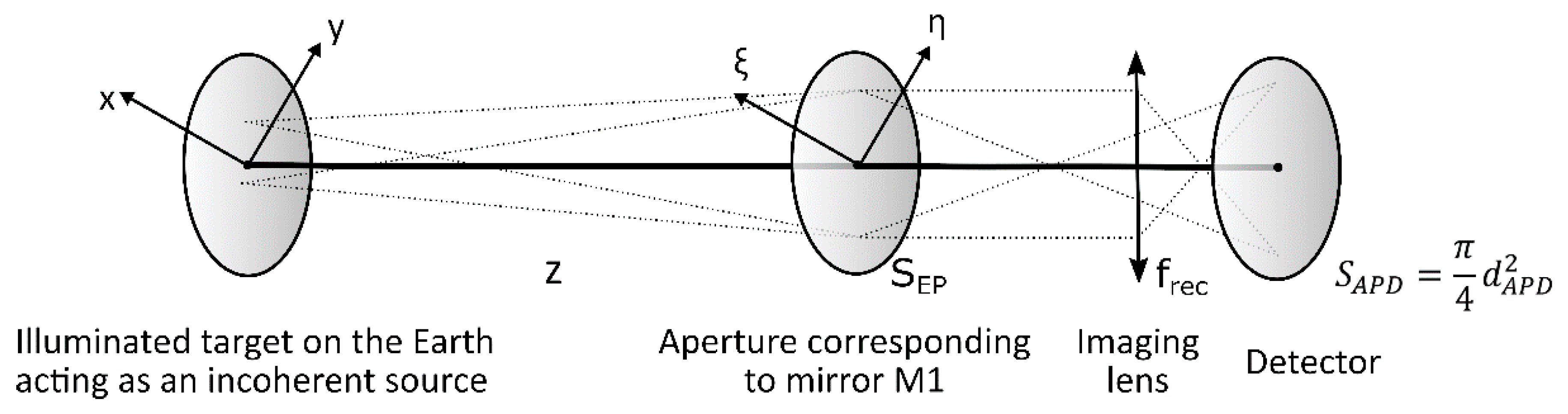
For satellite or airborne IPDA lidar observation, the ground is counted as a plane rough surface illuminated by a coherent source and it is modelled as an extended source of chaotic light of intensity IG (Δx, Δy, t) producing a fully-developed speckle pattern resulting from interference in the propagating space (Figure 1). The field of scattered light is observed at distance z of the rough surface and the area of coherence at this location is determined using results from Appendix A.
The instrument has relative speed to ground v. It emits wavelengths in (λon) and near (λoff) a methane multiplet. The emitted beam is polarized and its divergence is divbeam. The receiver telescope is an afocal design with huge magnification. It consists of two conical mirrors M1 and M2 plus an achromatised ocular lens which generates an image of the entrance pupil. The collecting mirror M1 is elliptical. To obtain a compact design, the secondary mirror M2 is close to M1, and M2 partly vignettes the entrance pupil. Up to the detector the focal length of the receiver chain is frec. A band pass filter is incorporated on the optical path to block the light outside a narrow window with size Lfilter. The incoming signal light scattered back by the earth is focused on the detector of diameter dAPD which collect also the calibration light from the energy monitoring path [12]. The use of the same detector for signal estimate and energy monitoring avoids variations in the optical-to-electrical response between the two, but the energy extracted from the emitted beam has to be reduced by several orders of magnitude to match the energy level of the lidar returns as the detector performances are for a limited energy range. For this purpose, integrating-spheres with fiber coupling are used [40]. The cut off frequency of the electronic detection is smaller than the sampling frequency νsample.
3. Speckle Contributions to Signal-to-Noise Ratio on MERLIN or CHARM-F XCH4 Measurements
Laser pulses energy are Gaussian distributed on the ground. The energy of scattered light is thus modeled as:
where I0 the mean intensity and σR the spatial standard deviation. That gives by integration in the field of view (FOV) of the receiver with Equation (A16) the effective area of the footprint looked as a secondary source for laser returns:
Solar energy is uniform in the FOV. The energy of scattered solar flux is thus modeled by a top hat distribution:
so, (still using Equation (A16)) the effective area for sun light is given by:
Because of the movement of the satellite (or of the aircraft) during the signal energy estimation there is time speckle renewal due to changes in the illuminating of the ground at the wavelength scale [36]. With deff the characteristic size of the coherent area (the diameter for a circular area), the characteristic time of this renewal is deff/v [32] which remains considerable even for space lidar (in the order of 0.1 ms). Moreover, as pulsed lidar are used, regardless of the laser beam characteristic time, there is a full coherence inside one pulse. There is no averaging of the interference pattern with increasing integration time as there is no more signal.
Table 3 provides both for MERLIN and CHARM-F the effective surface for incoherent source on ground, the coherence area, the coherence time and the number of speckles.
The number of temporal speckle for solar flux is estimated for a discretisation time δtdis settled between a tenth of the sampling time to a sampling time. Even if for simulation purposes the time signal is discretised at a tenth of the sampling time, for each discretisation interval there are several hundreds of temporal speckles for solar flux.
Subjective speckle for laser and solar fluxes are not to be counted as the detection optics is built in such a way that all the photons collected by the entrance pupil reach the detector. So, speckle only modulates the spatial distribution of the energy on the detector and not its integrated value.
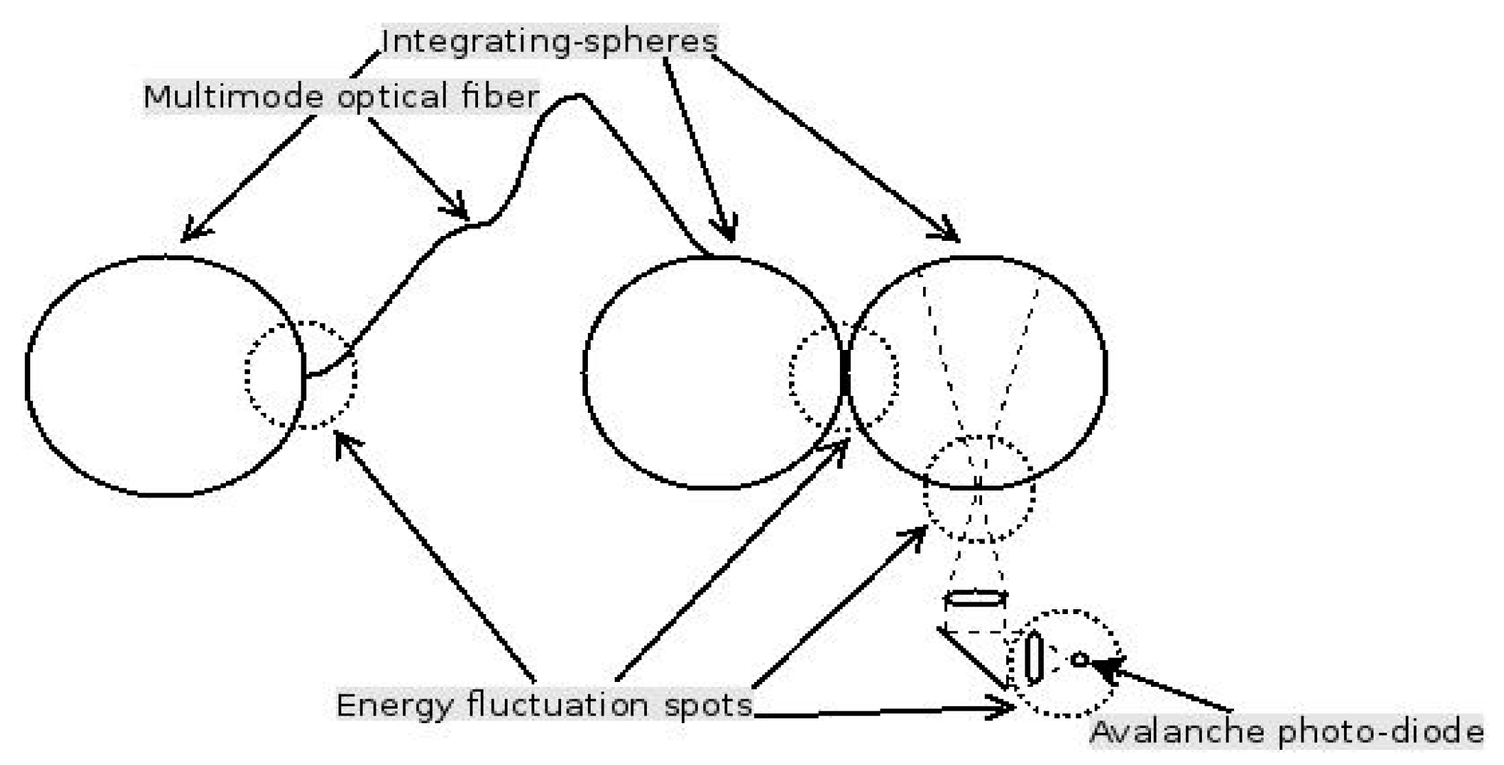
Along the optic calibration path (see Figure 2), speckle induces fluctuations of the energy amount at each location where there is energy dilution, specifically the output of the integrated spheres and the entrance of the optical fibers.
For CHARM-F it is assumed that the detector does not truncate the fiber output [14], but for MERLIN in order to avoid alignment issues, the illuminating area is larger than the detector size. Therefore, subjective speckle also occurs. For MERLIN, AIRBUS has done a dedicated study on preliminary design for this calibration path and estimated SNREon/Eoff around 43 mainly from detector and fiber entrance face [personal communication]. For CHARM-F, the SNREon/Eoff could be estimated from [40] around 59 mainly from fiber entrance face.
Table 4 summarizes SNR estimates obtained with Equation (4) and data from Table 3 for the different fluxes in the case of MERLIN and CHARM-F. Pon and Poff are polarized, Psun is not, Eon and Eoff neither because integrated-spheres depolarize [46]. The maximum number of backscattered photons for MERLIN has been estimated to less than 18000 and for CHARM-F it is about 3550 time more (because the distance between ground and the receiver is 8.5 km instead of 506.3 km). The relative random error (RRE) is the inverse of the SNR and can be expressed in percentage form.
Speckle noise is of the same order but smaller than shot noise for MERLIN lidar. Conversely, for CHARM-F lidar, speckle noise is dominant compared to shot noise which becomes negligible with the smaller distance between the receiver and the ground.
Using a mean value of 0.53 for DAOD and a mean value of 1780 ppb for methane content the random uncertainties coming from speckle on XCH4 estimated with value of Table 4 and Equation (7) are summarized in Table 5. Noise for 7 s average corresponds to 50 km average for MERLIN and to 2 km average for CHARM-F.
The random error of 5 ppb from speckle is compatible with the specification of MERLIN random error less than 22 ppb [2] but shows how difficult it will be to reach the target user requirement for random error estimated at 8 ppb.
4. Discussion and Conclusions
For any satellite or airborne IPDA lidar, speckle induces variability of incident energy on the detector both for atmospheric and energy monitoring branches. Subjective speckle has no impact on the energy absorbed by the detector as long as it does not truncate the energy collected. SNR from speckle can be estimated as above (Table 4) on a shot by shot basis. The associated noises are smaller with respect to the electronic noise, for which averaging is needed. There is no difficulty in calculating such an average for simulated data even if geophysical variability should be taken into account to be realistic [47]. But the noise correlation between the various samples describing one shot and between different shots must be included.
For signal path the speckle pattern changes like the target from one shot to another. If the speckle pattern changes there is no correlation between the noises. But for energy monitoring path, the speckle pattern may be highly correlated from one shot to another. And to limit speckle impact on random noise for XCH4 spatially averaged, it is necessary to either fully stabilize the speckle pattern, or to deliberately change it over time [48,49]. This second solution is easier to do on mobile lidar and the first one may induce systematic bias on the methane estimation. Using moving parts, specific systems have been designed to change speckle pattern between successive pulses. Tests with CHARM-F showed resulting noise exhibiting pure white noise behavior which can be reduced by averaging [40]. The introduction of such a mechanism prevents any correlation between speckle simulated noises for one shot and another [41].
Simulations of IPDA data with realistic speckle noise may be performed after computations similar to those in Section 3, and with the two hypotheses of full correlation for the samples of one shot (because the noise is fully correlated at this time scale as the speckle pattern is constant during the full registration of one pulse) and of full decorrelation between shots.
In summary, nothing has to be done for sun flux. Only Gaussian random noise has to be added, both on each sampling of energy monitoring fluxes and on each sampling of signal fluxes. Only one random draw is needed for energy monitoring path and signal path per shot. However, a new random draw is necessary for each shot because the speckle pattern vary from one pulse to the other according to the use of the decorrelation mechanism acting between two pulses.
For the MERLIN mission, the SNR on optical energy of backscattered signals due to speckle is around 60, always higher than the shot noise SNR which is less than 50. On the contrary for CHARM-F, speckle SNR is smaller than the shot noise SNR. Speckle occurring on the energy monitoring path is associated to pulse by pulse SNR about 40 for MERLIN (60 for CHARM-F) and so it is the dominant speckle impact even with a decorrelation mechanism. A Gaussian model of these noises has to be included in the Merlin simulator.
Author Contributions
Conceptualization, V.C.; Resources, F.G. and D.E.; Writing—original draft, V.C.; Writing—review & editing, V.C., F.G., D.E., O.C. and C.C.
Funding
This research received no external funding.
Acknowledgments
The authors acknowledge for fruitful exchanges the members of CNES MERLIN MAG. They also thank the whole bilateral MERLIN project team at CNES, DLR and AIRBUS DS and two anonymous reviewers for their careful reading of the manuscript and theirs’ relevant suggestions.
Conflicts of Interest
The authors declare no conflicts of interest.
Appendix A. Speckle Theory
The speckle theory has been developed by J. C. Dainty [30] and J. W. Goodman [31] from previous studies on coherent light [50]. For any beam, its intensity (or brightness) is defined from the amplitude of the electromagnetic wave u at location Pi and time ti as:
and its degree of first order coherence (g(1)) as the normalized first order correlation function between point P1 at time t1 and point P2 at time t2 [51]:
which vary between 0 for incoherent light and 1 for first order coherent light. In this equation (A2) g(1) is the spatial complex factor of coherence listed as μ (P1, P2) at a given time (t1 = t2) and the temporal complex degree of coherence listed as γt) at a given location (P1 = P2)). It measures the visibility of interference fringes. Similarly, the beam degree of second order coherence g(2) is defined as the normalized second order correlation function:
which vary between 1 and +∞.
A monochromatic beam is said chaotic when it can be represented as a Gaussian random process [52] resulting of the well-known random walk in the complex amplitude plane. Thermal light and coherent light after full scattering are chaotic lights. Chaotic light interferes with itself creating speckle pattern. The questions are to determine speckle sizes and the energy collected by a detector put in this speckle field.
For chaotic light, negative exponential relationship is found for the distribution of brightness:
where I0 is the statistical mean value of brightness. The most probable brightness for a speckle is zero and there are more dark speckles in the field than speckles of any other brightness, but there are also rare very bright speckles.
The mean intensity of illumination W for an area S during a time ΔT results from the integration of I(P; t) taking into account its spatial and temporal correlations is given by:
Similarly the second-order moment is given by:
A function S(P) with values between 0 and 1 allows to take into account differences in the contribution of the various points P of the area S to the signal e.g., the sensitivity of the detector or some movement of the detector during a window time ΔT. In that last case, for a movement in the y direction the function is:
The mean value W and the standard deviation σW are computed using M [31,37] defined by:
where and Λ(x) = 1 − |x| for |x| < 1, zero otherwise.
For chaotic light, the correlation functions verify the following relation [51]:
then the SNR is related to M by:
where P refers to the polarization index (P is defined for a wave as the ratio of the intensity of the polarized component to the total intensity, |P|= 1 if the light is fully polarized, P = 0 if it is not polarized). M is very well approximated as follow [31]
where
and
Using Wiener-Khintchine and Zernike-Van Cittern theorems, τc and Sc may be computed from the statistics properties of the complex amplitude of the incident light. The characteristic time can be computed from the spread of its frequencies [52]. For a Gaussian beam characterized by its standard deviation σν, characteristic time τc is given by:
and, for thermal light through a bandwidth filter of size Lfilter around mean frequency λ, the characteristic time τc is given by:
On a plane parallel to the emitting surface, the speckle dimensions can be computed from the brightness distribution of the emitted light on the scattering area [31]:
where z is the distance between the source and the detector and Seff the effective surface of the source corresponding to the emitting surface S in case of uniform illumination. The coherence area increases when the wave packet propagates as a result from the mix of waves coming from different points of the incoherent source. Assuming speckle and effective area are circular, the coherence area diameter is given by:
Furthermore, for a uniform illumination over a circular aperture with diameter d, Fourier transform gives the brightness distributed according to the first-order Bessel function of the first kind which first zero provides the size of coherence area:
The small difference between factor 1.27 and factor 1.22 is generally neglected, but in the first case the full area of coherence is counted and in the second case only the disc inside the main lobe. So, the first approach seems more accurate for energy estimation and the second for speckle size measurements.
For completeness, speckle sizes can be estimated not only on a plane parallel to the source but also on plane with angle θ from this direction (see Figure A1).
Figure A1.
Speckle pattern geometry [53].
Figure A1.
Speckle pattern geometry [53].

Then for an uniform source of chaotic light speckle sizes are given in the three directions by the following lengths [53]:
It is usual to name as “objective speckle” the pattern observed on a surface due to the interference of scattered waves coming from different points of a rough surface illuminated by laser light. When such a speckle pattern is imaged using an optical system, the entrance pupil may be counted as a source of chaotic light and the interference between waves coming from different points of the imaged plane build in the image plane a new speckle pattern named “subjective speckle”. The statistical properties of the scattering object determine speckle distribution in the observation plane (the area lightened). However, it is the size of the entrance pupil that determines speckles dimensions (the smaller the entrance pupil, the bigger the speckles). The subjective speckle size is obtained with the same relation than above, with the numerical aperture NA instead of the one-half angular aperture:
Thus, using the characteristics of a system which images the surface giving rise to the speckle—d the aperture diameter, f the focal distance and G the transverse factor of magnification—the coherence size is given by:
References
- Ciais, P.; Sabine, C.; Bala, G.; Bopp, L.; Brovkin, V.; Canadell, J.; Chhabra, A.; DeFries, R.; Galloway, J.; Heimann, M.; et al. Carbon and Others, Biogeochemical Cycles. In Climate Change 2013: The Physical Science Basis. Contribution of Working Group I to the Fifth Assessment Report of the Intergovernmental Panel on Climate Change; Stocker, T.F., Qin, D., Plattner, G.-n., Tignor, M., Allen, S.K., Boschung, J., Nauels, A., Xia, Y., Midgley, V.B., Eds.; Cambridge University Press: Cambridge, UK; New York, NY, USA, 2013; pp. 465–570. [Google Scholar]
- Ehret, G.; Bousquet, P.; Pierangelo, C.; Alpers, M.; Millet, B.; Abshire, J.B.; Bovensmann, H.; Burrows, J.P.; Chevallier, F.; Ciais, P.; et al. MERLIN: A French-German Space Lidar Mission Dedicated to Atmospheric Methane. Remote Sens. 2017, 9, 1052. [Google Scholar] [CrossRef]
- Kiemle, C.; Quatrevalet, M.; Ehret, G.; Amediek, A.; Fix, A.; Wirth, M. Sensitivity studies for a space-based methane lidar mission. Atmos. Meas. Tech. 2011, 4, 2195–2211. [Google Scholar] [CrossRef] [Green Version]
- Pierangelo, C.; Millet, B.; Esteve, F.; Alpers, M.; Ehret, G.; Flamant, P.; Berthier, S.; Gibert, F.; Chomette, O.; Edouart, D.; et al. MERLIN (Methane Remote Sensing Lidar Mission): An Overview. ILRC 27 EPJ Web Conf. 2016, 119, 26001. [Google Scholar] [CrossRef]
- Bousquet, P.; Pierangelo, C.; Bacour, C.; Marshall, J.; Peylin, P.; Ayar, P.V.; Ehret, G.; Bréon, F.M.; Chevallier, F.; Crevoisier, C.; et al. Error Budget of the MEthane Remote LIdar missioN and Its Impact on the Uncertainties of the Global Methane Budget. JGR Atmos. 2018, 123, 766–785. [Google Scholar] [CrossRef]
- Bode, M.; Alpers, M.; Millet, B.; Ehret, G.; Flamant, P. MERLIN: An integrated path differential absorption (IPDA) lidar for global methane remote sensing. In Proceedings of the International Conference on Space Optics—ICSO, Tenerife, Canari Island, Spain, 6–10 October 2014. [Google Scholar]
- Amediek, A.; Ehret, G.; Fix, A.; Wirth, M.; Büdenbender, C.; Quatrevalet, M.; Kiemle, C.; Gerbig, C. CHARM-F a new airborne integrated-path differential-absorption lidar for carbon dioxide and methane observations: Measurement performance and quantification of strong point source emissions. Appl. Opt. 2017, 56, 5182–5197. [Google Scholar] [CrossRef] [PubMed]
- Ingmann, P.; Bensi, P.; Durand, D. Six Candidate Earth Explorer Core Missions—Reports for Assessment: A-SCOPE—Advanced Space Carbon and climate Observation of Planet Earth; Clissold, P., Ed.; ESA Communication Production Office: Noordwijk, The Netherlands, 2008. [Google Scholar]
- Caron, J.; Durand, Y. Operating wavelengths optimization for a spaceborne lidar measuring atmospheric CO2. Appl. Opt. 2009, 48, 5413–5422. [Google Scholar] [CrossRef]
- NASA, Active Sensing of CO2 Emissions over Nights, Days, and Seasons (ASCENDS) Mission. NASA Science Definition and Planning Workshop Report. Available online: https://cce.nasa.gov/ascends (accessed on 10 September 2019).
- Ehret, G.; Kiemle, C.; Wirth, M.; Amediek, A.; Fix, A.; Houweling, S. Space-borne remote sensing of CO2, CH4, and N2O by integrated path differential absorption lidar: A sensitivity analysis. Appl. Phys. B 2008, 90, 593. [Google Scholar] [CrossRef]
- Amediek, A.; Fix, A.; Wirth, M.; Ehret, G. Development of an OPO system at 1.57 μm for integrated path DIAL measurement of atmospheric carbon dioxide. Appl. Phys. B 2008, 92, 295. [Google Scholar] [CrossRef]
- Abshire, J.B.; Riris, H.; Allan, G.R.; Weaver, C.J.; Mao, J.; Sun, X.; Hasselbrack, W.E.; Kawa, S.R.; Biraud, S. Pulsed airborne lidar measurements of atmospheric CO2 column absorption. Tellus B Chem. Phys. Meteorol. 2010, 62, 770–783. [Google Scholar] [CrossRef]
- Riris, H.; Numata, K.; Li, S.; Wu, S.; Ramanathan, A.; Dawsey, M.; Mao, J.; Kawa, R.; Abshire, J.B. Airborne measurements of atmospheric methane column abundance using a pulsed integrated-path differential absorption lidar. Appl. Opt. 2012, 51, 8296–8305. [Google Scholar] [CrossRef]
- Refaat, T.F.; Ismail, S.; Nehrir, A.; Hair, J.; Crawford, J.; Leifer, I.; Shuman, T. Performance evaluation of a 1.6-μm methane DIAL system from ground, aircraft and UAV platforms. Opt. Express 2013, 21, 30415–30432. [Google Scholar] [CrossRef] [PubMed]
- Abshire, J.B.; Ramanathan, A.; Riris, H.; Mao, J.; Allan, G.R.; Hasselbrack, W.E.; Weaver, C.J.; Browell, E.V. Airborne measurements of CO2 column concentration and range using a pulsed direct detection IPDA lidar. Remote Sens. 2014, 6, 443–469. [Google Scholar] [CrossRef]
- Refaat, T.F.; Singh, U.N.; Yu, J.; Petros, M.; Ismail, S.; Kavaya, M.J.; Davis, K.J. Evaluation of an airborne triple-pulsed 2 μm IPDA lidar for simultaneous and independent atmospheric water vapor and carbon dioxide measurements. Appl. Opt. 2015, 54, 1387–1398. [Google Scholar] [CrossRef] [PubMed]
- Yu, J.; Petros, M.; Singh, U.N.; Refaat, T.F.; Reithmaier, K.; Remus, R.; Johnson, W. An airborne 2-μm double-pulsed direct-detection lidar instrument for atmospheric CO2 column measurements. J. Atmos. Ocean. Technol. 2017, 34, 385–400. [Google Scholar] [CrossRef]
- Singh, U.N.; Refaat, T.F.; Ismail, S.; Davis, K.; Kawa, S.R.; Menzies, R.; Petros, M. Feasibility study of a space-based high pulse energy 2 μm CO2 IPDA lidar. Appl. Opt. 2017, 56, 6531. [Google Scholar] [CrossRef] [PubMed]
- Abshire, J.B.; Ramanathan, A.K.; Riris, H.; Allan, G.R.; Sun, X.; Hasselbrack, W.E.; Mao, J.; Wu, S.; Chen, J.; Numata, K.; et al. Airborne measurements of CO2 column concentrations made with a pulsed IPDA lidar using a multiple-wavelength-locked laser and HgCdTe APD detector. Atmos. Meas. Tech. 2018, 11, 2001–2025. [Google Scholar] [CrossRef]
- Wagner, G.A.; Plusquellic, D.F. Multi-frequency differential absorption LIDAR system for remote sensing of CO2 and H2O near 1.6 μm. Opt. Express. 2018, 26, 19420–19434. [Google Scholar] [CrossRef] [PubMed]
- Wagner, G.A.; Plusquellic, D.F. Ground-based, integrated path differential absorption LIDAR measurement of CO2, CH4, and H2O near 1.6 μm. Appl. Opt. 2016, 55, 6292–6310. [Google Scholar] [CrossRef]
- Spiers, G.D.; Menzies, R.T.; Jacob, J.; Christensen, L.E.; Phillips, M.W.; Choi, Y.; Browell, E.V. Atmospheric CO2 measurements with a 2 μm airborne laser absorption spectrometer employing coherent detection. Appl. Opt. 2011, 50, 2098–2111. [Google Scholar] [CrossRef]
- Menzies, R.T.; Spiers, G.D.; Jacob, J.C. Airborne laser absorption spectrometer measurements of atmospheric CO2 column mole fractions: Source and sink detection and environmental impacts on retrievals. J. Atmos. Ocean. Technol. 2014, 31, 404–421. [Google Scholar] [CrossRef]
- Sakaizawa, D.; Kawakami, S.; Nakajima, M.; Sawa, Y.; Matsueda, H. Ground-based demonstration of a CO2 remote sensor using a 1.57 μm differential laser absorption spectrometer with direct detection. J. Appl. Remote Sens. 2010, 4, 043548. [Google Scholar] [CrossRef]
- Sakaizawa, D.; Kawakami, S.; Nakajima, M.; Tanaka, T.; Morino, I.; Uchino, O. An airborne amplitude-modulated 1.57 μm differential laser absorption spectrometer: Simultaneous measurement of partial column-averaged dry air mixing ratio of CO2 and target range. Atmos. Meas. Tech. 2013, 6, 387–396. [Google Scholar] [CrossRef]
- Du, J.; Zhu, Y.; Li, S.; Zhang, J.; Sun, Y.; Zang, H.; Liu, D.; Ma, X.; Bi, D.; Liu, J.; et al. Double-pulse 1.57 μm integrated path differential absorption lidar ground validation for atmospheric carbon dioxide measurement. Appl. Opt. 2017, 56, 7053–7058. [Google Scholar] [CrossRef] [PubMed]
- Queißer, M.; Burton, M.; Fiorani, L. Differential absorption lidar for volcanic CO2 sensing tested in an unstable atmosphere. Opt. Express 2015, 23, 6634–6644. [Google Scholar] [CrossRef] [PubMed]
- Fiorani, L.; Santoro, S.; Parracino, S.; Nuvoli, M.; Minopoli, C.; Aiuppa, A. Volcanic CO2 detection with a DFM/OPA-based lidar. Opt. Lett. 2015, 40, 1034–1036. [Google Scholar] [CrossRef] [PubMed]
- Dainty, J.C. Laser Speckle and Related Phenomena; Springer science & business Media: Berlin, Germany, 1975. [Google Scholar]
- Goodman, J.W. Statistical Optics; John Wiley & Sons: Hoboken, NJ, USA, 1985. [Google Scholar]
- Ohtsubo, J.; Asakura, T. Velocity measurement of a diffuse object by using time-varying speckles. Opt. Quantum Electron. 1976, 8, 523–529. [Google Scholar] [CrossRef]
- Ostberg, K. Differential Absorption Lidar: Effects of Speckle Noise; Research Inst of National Defence Stockholm: Stockholm, Sweden, 1979. [Google Scholar]
- Flamant, P.H.; Menzies, R.T.; Kavaya, M.J. Evidence for speckle effects on pulsed CO2 lidar signal returns from remote targets. Appl. Opt. 1984, 23, 1412–1417. [Google Scholar] [CrossRef]
- Murty, S.R. Aerosol speckle effects on atmospheric pulsed lidar backscattered signals. Appl. Opt. 1989, 28, 875–878. [Google Scholar] [CrossRef] [Green Version]
- MacKerrow, E.P.; Schmitt, M.J. Measurement of integrated speckle statistics for CO2 lidar returns from a moving, nonuniform, hard target. Appl. Opt. 1997, 36, 6921–6937. [Google Scholar] [CrossRef]
- Nelson, D.H.; Walters, D.L.; MacKerrow, E.P.; Schmitt, M.J.; Quick, C.R.; Porch, W.M.; Petrin, R.R. Wave optics simulation of atmospheric turbulence and reflective speckle effects in CO2 lidar. Appl. Opt. 2000, 39, 1857–1871. [Google Scholar] [CrossRef]
- Chen, J.R.; Numata, K.; Wu, S.T. Error reduction methods for integrated-path differential-absorption lidar measurements. Opt. Express. 2012, 20, 15589–15609. [Google Scholar] [CrossRef] [PubMed]
- Refaat, T.F.; Singh, U.N.; Petros, M.; Remus, R.; Yu, J. Self-calibration and laser energy monitor validations for a double-pulsed 2-μm CO2 integrated path differential absorption lidar application. Appl. Opt. 2015, 54, 7240–7251. [Google Scholar] [CrossRef] [PubMed]
- Fix, A.; Quatrevalet, M.; Amediek, A.; Wirth, M. Energy calibration of integrated path differential absorption lidars. Appl. Opt. 2018, 57, 7501–7514. [Google Scholar] [CrossRef] [PubMed]
- Wenyi, H.; Jiqiao, L.; Yadan, Z.; Junfa, D.; Xiuhua, M.; Shiguang, L.; Junxuan, Z.; Xiaopeng, Z.; Weibiao, C. Analysis of energy monitoring for a double-pulsed CO2 integrated path differential absorption lidar at 1.57 μm. Appl. Opt. 2019, 58, 616–625. [Google Scholar] [CrossRef]
- Jacquinet-Husson, N.; Armante, R.; Scott, N.A.; Chedin, A.; Crépeau, L.; Boutammine, C.; Bouhdaoui, A.; Crevoisier, C.; Capelle, V.; Boonne, C.; et al. The 2015 edition of the GEISA spectroscopic database. J. Mol. Spectrosc. 2016, 327, 31–72. [Google Scholar] [CrossRef] [Green Version]
- Delahaye, T.; Maxwell, S.E.; Reed, Z.D.; Lin, H.; Hodges, J.T.; Sung, K.; Devi, V.; Warneke, T.; Tran, H. Precise methane absorption measurements in the 1.64 μm spectral region for the MERLIN mission. J. Geophys. Res. Atmos. 2016, 121, 7360–7370. [Google Scholar] [CrossRef] [PubMed]
- Delahaye, T.; Ghysels, M.; Hodges, J.T.; Sung, K.; Armante, R.; Tran, H. Measurement and modeling of air-broadened methane absorption in the MERLIN spectral region at low temperatures. J. Geophys. Res. Atmos. 2019, 124, 3556–3564. [Google Scholar] [CrossRef]
- Nicodemus, F.E. Directional Reflectance and Emissivity of an Opaque Surface. Appl. Opt. 1965, 4, 767–775. [Google Scholar] [CrossRef]
- McClain, S.C.; Bartlett, C.L.; Pezzaniti, J.L.; Chipman, R.A. Depolarization measurements of an integrating sphere. Appl. Opt. 1995, 34, 152–154. [Google Scholar] [CrossRef] [PubMed]
- Tellier, Y.; Pierangelo, C.; Wirth, M.; Gibert, F.; Marnas, F. Averaging bias correction for the future space-borne methane IPDA lidar mission MERLIN. Atmos. Meas. Tech. 2018, 11, 5865–5884. [Google Scholar] [CrossRef] [Green Version]
- Lowenthal, S.; Joyeux, D. Speckle Removal by a Slowly Moving Diffuser Associated with a Motionless Diffuser. J. Opt. Soc. Am. 1971, 61, 847–851. [Google Scholar] [CrossRef]
- Singh Mehta, D.; Naik, D.; Singh, R.; Takeda, M. Laser speckle reduction by multimode optical fiber bundle with combined temporal, spatial, and angular diversity. Appl. Opt. 2012, 51, 1894–1904. [Google Scholar] [CrossRef] [PubMed]
- Mandel, L.; Wolf, E. Coherence Properties of Optical Fields. Rev. Mod. Phys. 1965, 37, 231–287. [Google Scholar] [CrossRef]
- Loudon, R. The Quantum Theory of Light; Oxford University Press: Oxford, UK, 2000. [Google Scholar]
- Wang, Q. Discussion on the fully developed speckle field. Optik 2013, 124, 2948–2950. [Google Scholar] [CrossRef]
- Li, Q.; Chiang, F. Three-dimensional dimension of laser speckle. Appl. Opt. 1992, 31, 6287–6291. [Google Scholar] [CrossRef] [PubMed]
Figure 1.
Observation geometry scheme.

Figure 2.
Locations on optic calibration path from where speckle can contribute to noise.


Table 1.
MERLIN and CHARM-F lidars parameter values needed to compute speckle impacts on signal.
| Parameter | Symbol | MERLIN | CHARM-F |
|---|---|---|---|
| Distance between ground and receiver | z | 506.3 km | 8.5 km |
| Instrument speed relative from Earth | v | 7.6 km/s | 0.2 km/s |
| ON wavelength | λon | 1645.5518 nm | 1645.555 nm |
| OFF wavelength | λoff | 1645.8460 nm | 1645.860 nm |
| Polarization of the emitted beam | P | 1 | 1 |
| FWHM laser pulse energy density spectrum | dνl | 60 MHz | 50 MHz |
| Beam full divergence at e−2 at transmitter telescope output | divbeam | 0.18125 mrad | 3 to 6 mrad |
| Length of elliptical entrance pupil | LM1 | 0.7325 m | 0.06 m |
| Width of elliptical entrance pupil | lM1 | 0.69 m | 0.06 m |
| Obscuration of M1 by M2 | OM2 | 0.03% | 0.00% |
| Focal length of reception optics | frec | 0.4704 m | 0.0303 m |
| Avalanche photo-diode diameter | dAPD | 200 μm | 200 μm |
| Spectral filter width | Lfilter | 2 nm | 2 nm |
| Sampling frequency | νsample | 75 MHz = 1/13.3 ns | 100 MHz = 1/10.0 ns |
Table 2.
Some geometric quantities computed from MERLIN and CHARM-F lidars parameters.
| Quantity | Symbol | MERLIN | CHARM-F |
|---|---|---|---|
| Diameter at e−2 for energy distribution on ground | de2G = z divbeam | 91.8 m | 25.5–51.0 m |
| Diameter of the FOV on ground | dfov = z dAPD/frec | 215.3 m | 56.1 m |
| Effective size of the entrance pupil | SEP = π/4 LM1 lM1 (1-OM2) | 3850.5 cm2 | 28.2 cm2 |
Table 3.
Speckle characteristics for MERLIN and CHARM-F IPDA lidars (λ = 1645.7 nm).
| Speckle Characteristics | Symbol | MERLIN | CHARM-F |
|---|---|---|---|
| Effective surface on ground for laser fluxes | Sefflas ~ π/4 de2G2 | 6618.7 m2 | 510.7–2042.8 m2 |
| Effective surface on ground for solar flux | Seffsun = π/4 dfov2 | 36406.4 m2 | 2471.8 m2 |
| Coherence surface for laser fluxes | Sclas = 4/π (λ/divbeam)2 | 105 mm2 | 0.38–0.096 mm2 |
| Coherence surface for solar flux | Scsun = 4/π (λ × frec/dAPD)2 | 19 mm2 | 0.079 mm2 |
| Characteristic time for sun light | τcsun = 1/(Lfilter × c/λ2) | 4.52 10−3 ns | 4.52 10−3 ns |
| Number of spatial speckles for laser fluxes | Mslas = 1 + SEP/Sclas | 3668 | 7440–29449 |
| Number of spatial speckles for solar flux | Mssun = 1 + SEP/Scsun | 20267 | 35786 |
| Number of temporal speckles for laser fluxes | Mtlas = 1 | 1 | 1 |
| Number of temporal speckles for solar flux | Mtsun = 1 + δtdis/τcsun | 296–2951 | 222–2213 |
Table 4.
SNR (signal to noise ratio) and RRE (relative random error) from speckle for different in the case of MERLIN and CHARM-F lidars.
Table 4.
SNR (signal to noise ratio) and RRE (relative random error) from speckle for different in the case of MERLIN and CHARM-F lidars.
| MERLIN | CHARM-F | MERLIN | CHARM-F | ||
|---|---|---|---|---|---|
| SNRPon/Poff | 61 | 86 | RREPon/Poff | 1.6% | 1.2% |
| SNRPsun | 3470–10948 | 3986–12585 | RREPsun | 0.0% | 0.0% |
| SNREon/Poff | 43 | 59 | RREEon/Eoff | 2.3% | 1.7% |
| SNRsn | <49 | about 3000 | RREsn | >2.0% | 0.0% |
Table 5.
Random noise on XCH4 due to speckle for MERLIN and CHARM-F lidar.
| MERLIN | CHARM-F | |
|---|---|---|
| Noise for one shot | 60 ppb | 41 ppb |
| Noise for a 7s average | 5 ppb | 3 ppb |
© 2019 by the authors. Licensee MDPI, Basel, Switzerland. This article is an open access article distributed under the terms and conditions of the Creative Commons Attribution (CC BY) license (http://creativecommons.org/licenses/by/4.0/).
Share and Cite
MDPI and ACS Style
Cassé, V.; Gibert, F.; Edouart, D.; Chomette, O.; Crevoisier, C. Optical Energy Variability Induced by Speckle: The Cases of MERLIN and CHARM-F IPDA Lidar. Atmosphere 2019, 10, 540. https://doi.org/10.3390/atmos10090540
AMA Style
Cassé V, Gibert F, Edouart D, Chomette O, Crevoisier C. Optical Energy Variability Induced by Speckle: The Cases of MERLIN and CHARM-F IPDA Lidar. Atmosphere. 2019; 10(9):540. https://doi.org/10.3390/atmos10090540
Chicago/Turabian StyleCassé, Vincent, Fabien Gibert, Dimitri Edouart, Olivier Chomette, and Cyril Crevoisier. 2019. "Optical Energy Variability Induced by Speckle: The Cases of MERLIN and CHARM-F IPDA Lidar" Atmosphere 10, no. 9: 540. https://doi.org/10.3390/atmos10090540
Note that from the first issue of 2016, this journal uses article numbers instead of page numbers. See further details here.