Comparison of Particulate Mercury Measured with Manual and Automated Methods

Abstract
: A study was conducted to compare measuring particulate mercury (HgP) with the manual filter method and the automated Tekran system. Simultaneous measurements were conducted with the Tekran and Teflon filter methodologies in the marine and coastal continental atmospheres. Overall, the filter HgP values were on the average 21% higher than the Tekran HgP, and >85% of the data were outside of ±25% region surrounding the 1:1 line. In some cases the filter values were as much as 3-fold greater, with <5% of the points falling on the 1:1 line. A common characteristic in all seasons was that the Tekran only yielded a total of 6 data points above 1 part per quadrillion by volume (ppqv) (i.e., ∼4% of the observations), and had ∼25% of its measurements as below the limit of detection (<0.1–0.2 ppqv). In comparison, the filter always had HgP detectable above the blank level of 0.05 ppqv. The aerosol size distribution of HgP did not appear to be a major factor in the discrepancies between the two methods. The peaks in filter HgP were always concomitant with enhanced mixing ratios of selected hydrocarbons, halocarbons, and oxygenated compounds. Backward trajectories suggested that the peaks in all chemical compounds were primarily anthropogenic, and tracers indicated a combustion signature. Since the Tekran was typically unresponsive to these pollution episodes, detailed investigation of aerosol passing efficiency and the instrument response to different aerosol types should be investigated.1. Introduction
Accurate measurements of mercury chemical speciation are required to understand correctly its cycling and lifetime in the atmosphere. In the atmosphere mercury exists in diverse chemical forms that are comprised of gaseous elemental mercury (Hg0), reactive gaseous mercury (RGM = HgCl2 + HgBr2 + HgOBr + …), and particulate-phase mercury (HgP). Compared to Hg° and RGM, HgP has received relatively little attention. Measurement of HgP requires either sampling with filters [1,2] or application of an automated Tekran model 1135 in conjunction with the Tekran model 2537 cold vapor fluorescence detection system [3-5]. The Tekran system is commonly employed to determine speciated atmospheric mercury world-wide.
The filter method could be prone to both positive and negative artifacts such as adsorption of RGM onto collected particulates [6] or loss of mercury from collected particulates when sampling times of more than a few hours are employed [7]. The Tekran system may have artifacts related to phase partitioning that varies with temperature [8]. An intercomparison conducted at Mace Head, Ireland, showed that HgP measured by participating groups was highly variable and at times different by nearly an order of magnitude [9]. Together, this limited work on HgP suggests that current methodologies for HgP measurements need to be investigated rigorously.
Measurements of HgP in southern Québec, Canada, yielded an average concentration of 26 ± 54 picograms (pg) m−3 [10]. There was a sharp seasonal variation, with the largest concentrations occurring in wintertime. Similar concentrations were found at two sites in Nevada, United States, with average HgP being 9 ± 7 pg m−3 and 13 ± 12 pg m−3 [11]. The Ohio River Valley in the United States has a large number of coal-fired power plants, but HgP was relatively low and averaged 5.29 ± 6.04 pg m−3 [12]. In the highly populated and industrial city of Shanghai, China, HgP ranged from 0.07 nanograms (ng) m−3 to 1.45 ng m−3 with an average of 0.56 ± 0.22 ng m−3 at one site, and 0.20 to 0.47 ng m−3 with an average of 0.33 ± 0.09 ng m−3 at another site [13]. These are among the highest values of ambient HgP reported in the literature. In contrast, in continental outflow from China at Okinawa Island, Japan, HgP averaged only 3.0 ± 2.5 pg m 3 [14].
Weekly measurements of HgP on Bermuda yielded low concentrations with an average of 1.3 ± 1.7 pg m−3 and a range of from the limit of detection (0.5 pg m−3) to 5.2 pg m−3 [2]. These values are consistent with other measurements over the remote ocean [15,16], but lower than at coastal locations. For example, the average HgP value along Chesapeake Bay was an order of magnitude larger at 27 ± 48 pg m−3 [2].
In the marine boundary layer (MBL) models show that the production of RGM should be enhanced due to the presence of halogens, especially Br and Cl radicals [17,18]. The deposition velocity of RGM is also 5–10 times higher than HgP over land [19], and is likely even greater over the ocean. At Bermuda RGM averaged 50 ± 43 pg m−3, which was 30–40 times higher than HgP. In comparison, the ratio of RGM/HgP is <5 at many remote terrestrial locations [2].
Our group has been conducting measurements of Hg° in coastal New Hampshire at Thompson Farm since November 2003 and on Appledore Island in the Gulf of Maine since July 2005 [20]. Recently, RGM and HgP measurements were added to both sites [21,22]. Currently, we are investigating the phase partitioning and cycling of atmospheric mercury in the marine boundary layer at Appledore Island. Intensive field campaigns were conducted in summer 2009, winter 2010, and spring 2010 which involved measurements of bulk filter HgP, size fractionated HgP, and HgP with a Tekran model 1135. An important feature of these studies was that measurements were conducted in the marine and continental atmospheres to ascertain differences in phase partitioning and cycling in these two environments. Here we report seasonal comparisons of HgP measured with the manual filter method and the automated Tekran system.
2. Results and Discussion
2.1. Campaign Details
During summer 2009 studies were conducted on Appledore Island in the Gulf of Maine and at and the inland site Thompson Farm. Tekran speciated atmospheric mercury systems were operated continuously at each site. At both sites two cascade impactors were run twice for seven days each. Bulk filter samples were collected with three hour time resolution. Ozone (O3) and carbon monoxide (CO) were measured with one minute time resolution. Stainless steel canisters were used to collect whole air samples once an hour for determination of hydrocarbons, halocarbons, alkyl nitrates, and selected sulfur gases. The analyses were conducted in the trace gas laboratory at the University of New Hampshire. At Thompson Farm ∼200 trace gases are measured year-round. During the intensive period in summer 2009 canister samples were collected and continuous measurement of oxygenated compounds was conducted using proton transfer reaction mass spectrometry. The various scenarios of data availability during each intensive period are summarized in Table 1.
2.2. Campaign Results
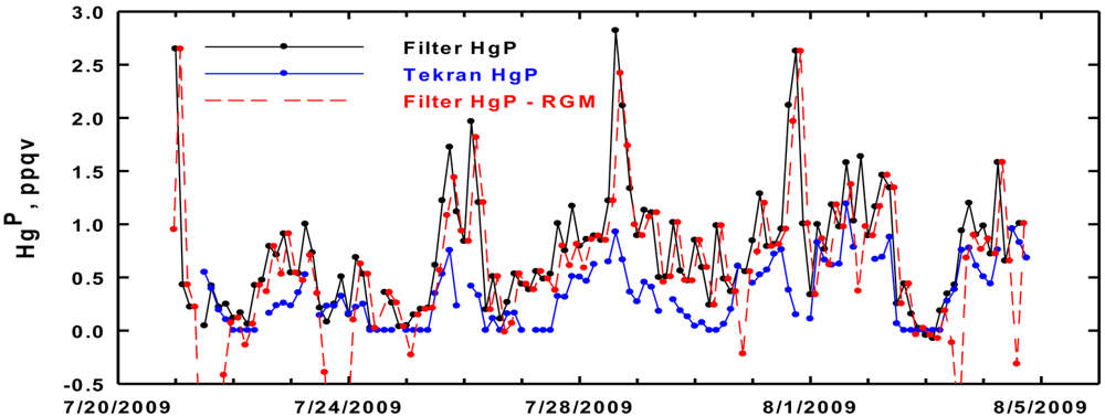
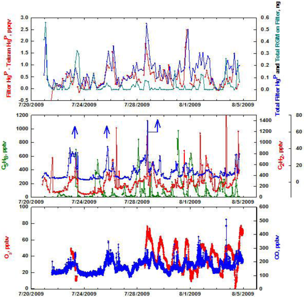
The time series record of HgP measured on Appledore Island in summer 2009 with the Tekran and filter methods are shown in Figure 1. We report HgP in terms of its mixing ratios in parts per quadrillion by volume (ppqv). Further, we note that 1 ng m−3 of Hg is equal to 112 ppqv. The Tekran rarely found HgP to be >1 ppqv, while the filter determined values were up to 3 ppqv on several occasions. To check for a positive artifact with the filter measurements from uptake of RGM, we also show in Figure 1 HgP measured with the filter minus the corresponding integrated RGM value. It is apparent that the higher values obtained with the filter is not due to uptake of RGM. It is interesting that at times the two measurements show trends in the opposite direction and that the Tekran often was reading zero ppqv for hours at a time. The calibration of the Tekran was checked using a Tekran model 2505 Saturated Mercury Vapor Calibration Unit (i.e., direct injections from the headspace of a thermoelectrically cooled Hg° reservoir) and it was found to be within ±2%. Thus, calibration was ruled out as a cause for the discrepancies.
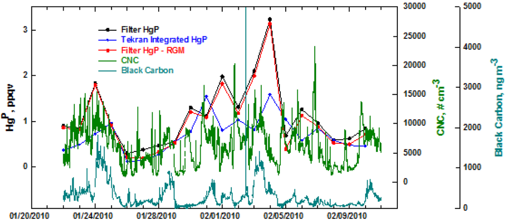
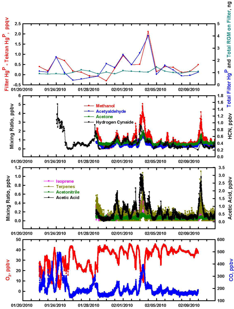
The data for HgP at Thompson Farm in winter is presented in Figure 2. The Tekran data was integrated to correspond better to the 24 hour filter samples. In general, the trends in the two HgP measurements were similar over the study period. Although there was better agreement in the two measurements of HgP in winter compared to summer, the Tekran only found HgP to be >1 ppqv two times. As in summer, there seems to be little influence of RGM on the filter-based HgP measurements. During the first couple of days of the study period there was close correlation with HgP and condensation nuclei (CNC)-black carbon. Afterwards, the three aerosol components exhibited individual characteristics suggesting that occasionally HgP was probably associated with black carbon. The bulk CNC also showed limited correspondence with HgP, which is probably not surprising considering the ultra-trace quantities of HgP in the atmosphere.
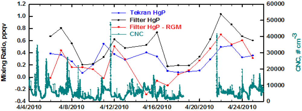
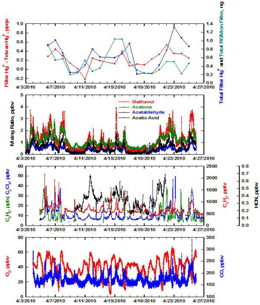
In springtime the situation was much different in that the two methods for measuring HgP tracked each other throughout the entire study period (Figure 3). However, overall the filter still yielded higher values of HgP compared to the Tekran. The same pattern emerged with the largest difference in the two values occurring when the filter yielded the highest mixing ratios of HgP. As was the case in winter, there was little correspondence between HgP and CNC. In springtime a positive artifact from RGM uptake on the filter could be a problem. When the total RGM passing through the filter was subtracted from the filter HgP it resulted in some values that were close or even significantly less than the Tekran HgP. Since this was not the case in the other seasons, it is caused by the highest annual RGM values occurring in spring (Table 2) [21].
A statistical summary of the seasonal data is presented in Table 2. We estimated that the filter data has an overall uncertainty of ∼±20%. To arrive at this estimate we propagated the errors associated with the analytical analysis, variability in the filter blank, multiple analyses of sample extracts, and the flow meter uncertainty. The accuracy of the filter HgP should be better than 5% since a certified reference was used in the analysis. The uncertainty of the Tekran unit is not well established, but periods of relatively constant ambient HgP mixing ratios indicate that it could be as good as ∼±5%. As an example of this, look at the variation in the Tekran HgP data from April 17 to April 20 in Figure 3. Although the mixing ratios are very low, the Tekran provided consistent values over this time period. In addition, the blank subtraction was essentially zero except for a few instances. Thus, a high blank was not responsible for the lower Tekran values of HgP. However, a better estimate of it should be obtained by operating two units side-by-side. We intend to do this in the future. Based on these uncertainty estimates, it is readily apparent that the filter yielded higher values of HgP than the Tekran unit. The seasonal comparison of HgP values determined with the filter show that while winter has the highest mixing ratios, summer is lower by ∼25% and spring ∼40%. A much different picture results from the Tekran data. Winter clearly stands out as the highest, with summer and spring lower by ∼60%. The greatest difference in the filter and Tekran HgP values occurred in the marine environment. This is likely caused by the presence of coarse sea salt aerosol which is probably not passed with high efficiency through the RGM denuder. The size distribution of HgP determined with cascade impactor sampling showed that ∼90% of the HgP was contained in aerosols with aerodynamic diameters > 2 micrometer (μm) at Appledore Island [22]. Thus, we attribute the 3-fold lower Tekran mixing ratios partially to this phenomenon. This is a large enough difference to inhibit accurate assessment of atmospheric mercury cycling and lifetimes in the marine boundary layer.
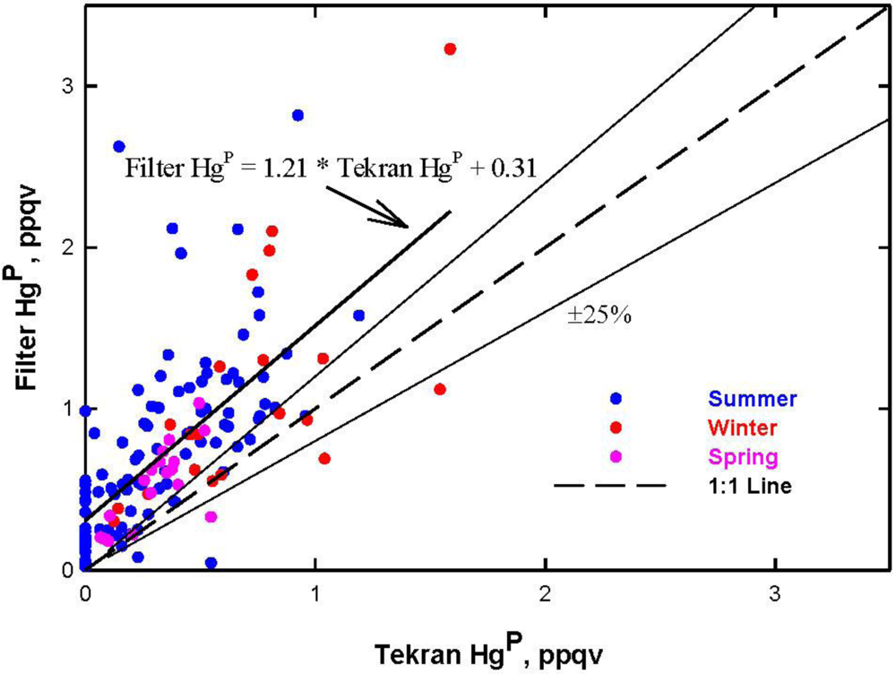
A summary plot is presented in Figure 4 which shows the seasonal relationships between filter HgP and the integrated Tekran HgP. We did not observe loss of mercury from the three-hour collection time periods for the filter, but the 24-hour and cascade impactor samples did have measurable losses presumably from halogen reactions [7]. This is discussed in detail in the companion paper by Feddersen [22]. We note that despite the losses from the 24-hour filters, the filter data were still provided higher mixing ratios of HgP as shown below.
The summer and winter data are the most disparate, while the spring data were more comparable. Overall, the filter HgP values were on the average 21% higher than the Tekran HgP, and >90% of the data lie outside of ±25% region surrounding the 1:1 line. In some cases the filter values were as much as 3-fold greater, with <5% of the points falling on the 1:1 line. A common characteristic in all seasons was that the Tekran only yielded a total of 6 data points above 1 ppqv (i.e., ∼4% of the observations), and had ∼25% of its measurements as below the limit of detection (<0.1–0.2 ppqv). In comparison, the filter always had detectable HgP above the blank level of 0.05 ppqv, and was undenuded to minimize positive artifacts from O3 reactions [23].
3. Discussion
The top panel of Figure 5 shows summer data at Appledore and we present some key relationships for the two measurement techniques of HgP First, the difference between the filter and Tekran HgP values has a median of 0.35 ppqv, and ranges from zero to 2.5 ppqv. There are only two data points (on July 21 and 23) where the Tekran HgP was greater than HgP measured with the filter. The largest differences occurred when the filter-based HgP produced the highest mixing ratios. Second, the total ng of Hg on the filter was calculated and compared to the total ng of RGM if the filter had retained it with 100% efficiency throughout the whole sampling interval. Early and late in the sampling period the amount of RGM would have been equal to or greater than the total amount of filter measured HgP. Throughout the rest of the sampling time frame, including the two largest peaks in HgP, RGM would seem to be a non-issue. We conclude that a positive RGM artifact is possible occasionally, but in general it does not appear to be a major problem.
In the middle panel of Figure 5 the time series of selected hydrocarbons and halocarbons are depicted over the two week sampling interval. Isoprene (C5H8) is a tracer of biogenic emissions, or continental air. Acetylene (C2H2) is an indicator of combustion, and tetrachloroethylene (C2Cl4) is emitted from urban sources such as dry cleaning [24]. It is clear that biogenic emissions are not associated with the largest peaks in HgP. The spike in HgP on July 28 also has concomitant peaks in C2H2 and C2Cl4 that suggest the HgP might be derived from urban activities. There is also significant O3 associated with this episode (Figure 5, bottom panel). Other large peaks in HgP on July 21 and 31 do not appear to have subsequent peaks in any of the tracer compounds, although the 31st also has elevated O3 and CO. For the closely spaced double peaks in HgP around July 26, C2Cl4 showed similar albeit not identical ones. Interestingly, the sustained peak in C2Cl4 around July 23 shows little influence on HgP levels. Apparently there is not a clear signal in the source of the high HgP at Appledore Island. Urban sources could account for a fraction of the elevated levels, but the picture is far from being straightforward.
Backward trajectories were calculated for HgP peaks that occurred on July 21, 28, and 31 at Appledore Island. The trajectories indicate that these air masses were likely influenced by urban/industrial sources along the U.S. east coast. The July 22 case showed an enhanced and sustained elevation in C2Cl4, an urban tracer, but little increase in HgP. The trajectories indicate the possibility that the air passed east of Boston and might not have been directly affected by local emission sources.
In Figure 6 we present the wintertime relationship between total ng of HgP on the filter and total ng RGM Hg if it was retained 100% on the filter. There are a few instances where a positive RGM artifact could be important, but in general it does not appear to be a factor. The two largest peaks in filter HgP, on January 24 and February 4, have concurrently high mixing ratios of many oxygenated compounds and hydrogen cyanide (HCN). The largest peak on February 4 exhibited biomass burning characteristics with concomitant 1 ppbv enhancements in HCN and acetonitrile (CH3CN). Acetic acid (CH3COOH) was also highly elevated and it is known to have biomass burning as a source [25]. Surprisingly, the biogenic compounds isoprene (C5H8) and terpenes were enhanced 0.5 and 1 ppbv respectively in the middle of winter. These compounds have relatively short lifetimes, and in winter they are usually near their limit of detection at Thompson Farm [26]. Backward trajectories indicate that the air originated over central Canada. However, Canadian fire count records indicated that there no wildfires burning there for weeks either side of February 4 ( www.ciffc.ca/index.php?option=com_content&task=view&id=26&Itemid=28). In addition, it is unlikely that the biomass-like emissions could be attributed to emissions from a coal-fired steam power plant since mixing ratios of CO2 and SO2 (not shown) were flat throughout this time interval.
Particularly perplexing is the source of the enhanced biogenic compounds. Air temperature varied from −1 to −10 °C on February 4 at Thompson Farm. This would seem to rule out a rare warm winter day with a spike in biogenic emissions. One possible source could be local wood burning in wood stoves and fireplaces, but nitric oxide (NO) and CO exhibited low and flat mixing ratios on February 4th. Thus, it is unclear as to the source(s) of the enhanced HgP and other chemical species.
The two other largest peaks in filter HgP that occurred on January 24 and February 1 have source regions over northern New England and the Ohio Valley area respectively. These peaks also appear to contain biomass burning characteristics but again little NO. In winter the lifetime of NO is about 1.5 days [27], which opens up the possibility of aged biomass burning emissions from wood stoves and fireplaces across the source regions. This could also explain the peak in HgP on February 4.
In springtime the variations in filter HgP were tracked well by C2H2, C2Cl4, oxygenated compounds, and CO (Figure 7). In general, when these compounds indicated pollution plumes were present, the filter HgP was also enhanced. The correspondence with C5H8 was marginal, with better correlations with combustion and anthropogenic tracers. There are peaks in O3 that correspond to the pollution plumes, and indicate active photochemistry was occurring. The diurnal trend in O3 is caused by production in daytime and deposition and titration at night under the nocturnal inversion [28]. The active photochemistry and presence of marine influences periodically at Thompson Farm in springtime produces the highest RGM mixing ratios during this season [29]. In fact, during April 14–16 the RGM was greater than the HgP measured with either method. The filter HgP during this time period is particularly prone to a positive artifact from RGM uptake on the filter during sampling. Note that the filter and Tekran HgP data are very similar during this time period and a t-test showed that they were not statistically different (p = 0.01). Since presumably the Tekran HgP is not subject to interference from RGM, this suggests the filter data were not impacted by an RGM positive artifact. In the laboratory we flowed Hg0 and HgCl2 in zero air (∼200 ppqv) from a permeation source through blank fluoropore filters and did not observe uptake of Hg0 or RGM by the Teflon filter. Thus, if uptake occurs under ambient conditions it must be caused by absorption/reaction with collected aerosols.
The four largest peaks in filter HgP occurred on April 7, 12, 16, and 22 in spring 2010. Three of these peaks had entirely different source regions based on 24-hour backward trajectories. The trajectories on April 7 and February 3 indicate that the pollution including HgP likely originated from anthropogenic sources in the Ohio Valley and Northeast urban corridor. On April 16 the high HgP probably can be attributed to local Boston sources. The peak on April 12 is uncertain to its source, and has the same source region as the winter peaks in HgP. Nonetheless, it appears that combustion, whether it is natural or anthropogenic, is a common source for HgP.
The size distribution of the HgP is reported in a companion paper by Feddersen et al. [22]. We briefly summarize the salient results here. In summer, the size distribution of HgP was mainly in the coarse (i.e., sea salt) fraction (>1 μm) between 2–10 μm at both Appledore Island and Thompson. This was shifted almost entirely to the fine fraction (<1 μm) below 0.5 μm in winter, with little detectable in the coarse sizes. In spring, there was a mixture of fine and coarse fractions. The coarse aerosols at both locations are dominated by sea salt, which is rarely present at Thompson Farm in winter. Together the results of this work and that of Feddersen et al. [22] indicate that the consistently lower HgP measured by the Tekran cannot be explained solely by poor passing efficiency of coarse aerosols in the automated unit. We have demonstrated that the summer and winter data are of similar disparities, yet each season is dominated by different aerosol size preferences for HgP. A possible explanation for the lower HgP values obtained with the Tekran unit is volatilization of Hg0/RGM from aerosols as they pass through the heated RGM denuder. This could occur as water is volatilized with associated release of Hg0/RGM back to the gas phase [30].
We examined the data for possible artifacts related to variations in relative humidity. At Appledore Island the humidity is more-or-less constant at about 80%. At Thompson Farm the relative humidity reaches 100% on most summer nights and decreases to half that in daytime. The Tekran data and the difference between the filter and Tekran were examined for a humidity influence. As aerosols passed through the heated RGM denuder, water might evaporate from aerosols with associated mercury yielding low HgP for the Terkan system. However, we could not identify any influence of humidity, and concluded that this was of minor importance.
4. Experimental Section
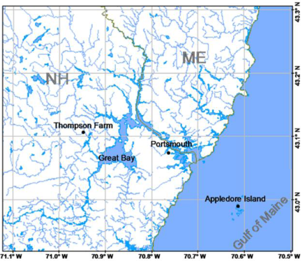
Two sites in the AIRMAP observing network ( www.airmap.unh.edu) were utilized for measurements of speciated atmospheric mercury. The first was at Thompson Farm (43.1078°N, 70.9517°W) which is located about 25 km inland from the Atlantic coastline. The second was on Appledore Island (42.97°N, 70.62°W) about 12 km offshore from New Hampshire in the Gulf of Maine. The geographic locations of these sites are shown in Figure 8. During certain time periods the Thompson Farm location is impacted by a marine influence, as indicated by the presence of tracer compounds such as CHBr3 and DMS [31,32]. Similarly, Appledore Island is under continental influence ∼30% of the time during summertime [33]. In general, wind speeds were only a few m s−1 during the campaigns.
At both sites we operate a Tekran system which consists of a model 1130 to measure RGM, a model 1135 to measure HgP, and 2537A cold vapor fluorescence detector. On Appledore all instruments are powered year-round by electricity generated by a custom wind turbine system [34]. Elemental Hg was quantified with a five minute time resolution. Reactive Hg and HgP were determined using a two hour sampling and one hour flushing and desorption sequences. The instruments were configured and operated identically at both sites according to the U.S. Environmental Protection Agency Standard Operating Procedures for Analysis of Gaseous and Fine Particulate-Bound Mercury [35], with one modification. Instead of using the Tekran commercial water removal cartridge system, we developed a custom cold finger unit which operates autonomously only producing water as a waste by-product. The system is extremely clean and we believe that it helps keep the blank on the speciated measurements at zero. Thus, blank subtraction is rarely required.
Calibration of the 2537A unit was conducted automatically every 24 desorption cycles, and this was verified every six months using a Tekran model 2505 Saturated Mercury Vapor Calibration Unit (i.e., direct injection from the headspace of a thermoelectrically cooled Hg0 reservoir) to confirm absolute calibration.
The Tekran units are typically equipped with an elutriator inlet with an acceleration jet to remove aerosols >2.5 μm so that only fine HgP is measured. This is not a desirable design, especially in the marine environment with sea salt in the 2–10 μm range. Since our goal was to elucidate cycling of mercury, the total amount of mercury in the aerosol phase must be determined. We replaced the elutriator in both model 1130 units with one that contained no impaction plate to facilitate collection of coarse aerosols on the quartz frit in the Tekran 1135. The face velocity through the quartz frit was ∼3.2 L cm−2 min−1, a much higher rate than through the filters at ∼1.1 L cm−2 min−1. At a flow rate of 10 standard liters per minute through the RGM denuder it is highly likely that some of the coarse aerosols will still be lost. However, without completely modifying the instrument this is the best that one can do, and our goal was to evaluate the Tekran system in a likely configuration to be used by researchers.
To help evaluate the accuracy of the Tekran HgP measurements, HgP was also determined using collection of bulk aerosols on Teflon filters. The filter was held upside down in a delrin housing and was situated ∼50 cm away from the inlet of the Tekran unit. We used Millipore fluoropore filters of 90 mm diameter and a pore size of 1 μm. The flow meters were calibrated just prior to the campaigns and they were within ±2% at the flow rates used in this study. Prior to sampling these were cleaned in 12 hour acid soaks of 30% HNO3 and 25% HCl. For sampling the filters were placed in custom delrin holders and ambient air flowed through them at ∼120 standard liters per minute. The holders were washed with soapy deionized water and then soaked 12 hours in 5% HCl. Blank filters went through the same handling process in-between each actual ambient sample. Samples and blanks were stored in clean room bags. Extracts were stored Teflon bottles that were soaked 12 hours in 50% HNO3, another 12 hours in 30% HCl, and finally soaked for 5 days in 5% HCl. Filter extractions were conducted using 1.5% BrCl and HCl for 24 hours. They were then diluted to 0.5% BrCl and HCL for analysis. The average blank filter contained 25 pg of Hg, while the samples contained up to 100 times more Hg. Thus, the blank corrections were essentially in the background noise and contributed little to the overall uncertainty of the ambient measurements.
Analysis of these samples for Hg was via acid extraction and cold vapor atomic fluorescence using a Tekran Series 2600 System. Calibration standards were prepared from a 1000 ppm Hg0 in 3% HNO3 Atomic Absorption solution purchased from Ricca Chemical Company. A certified reference material, ORMS-4 (Hg in water), purchased from the National Research Council Canada was utilized as an external standard. The analytical precision of repeated determinations of the ambient samples was 5–10%.
Ozone was measured at each site using UV photometric detection at 254 nm with a Thermo Environmental Instruments model 49C-PS. The limit of detection was ∼1.0 ppbv. Instrument zeroing and calibration was achieved routinely by utilizing zero air and an internal primary O3 source, respectively. Carbon monoxide was measured with an extensively modified Thermo Environmental Instruments model 48CTL. The technique uses a filter correlation method based on absorption of infrared radiation at 4.6 μm. Calibration was conducted using standard addition on ambient air from a CO primary standard of ∼5 ppmv obtained from Scott Marrin, Inc. (NIST traceable ±2%). The addition was dynamically diluted to provide a spike of ∼300 ppbv. Calibration was performed every 6.25 hours. The limit of detection was ∼20 ppbv. More details of these measurement techniques are presented in Mao and Talbot [36].
A condensation nuclei counter was utilized to measure aerosol number density. The unit was a TSI model 3022A, which was modified to automatically drain and refill the butanol reservoir to remove daily water contamination. The data were averaged to one minute and correspond to individual aerosol particles with a size range of 7 nanometer (nm) to 3 μm with an efficiency of 50% between 7 nm and 15 nm and greater than 90% above 15 nm. The instrument counts aerosol particles up to concentrations of 1 × 107 cm−3 using standard optical methods. Black carbon was measured using a Magee Scientific aethalometer with light attenuation at 880 nm. More details of these aerosol measurements can be found in Ziemba et al. [37].
For the HCN measurements at Thompson Farm, a cryogen-free concentration system coupled to gas chromatograph (GC) equipped with a flame thermionic detector (FTD) was employed. The system was designed for dual stage trapping such that there were two individual dewars containing cold regions—the first cold region was for water management, while the second cold region was used for sample enrichment. Ambient air was drawn from the main sampling manifold using a single-head metal bellows pump and directed to the concentration system. A 250 cm3 aliquot of air was first dried by passing it through an empty 20 cm × 0.3175 cm i.d. Silonite-coated loop held at −15 °C and then concentrated at −130 °C in a 20 cm × 0.3175 cm i.d. Silonite-coated loop packed with 1 mm diameter glass beads. After sample enrichment, the loops were heated to 80 °C and the sample was injected onto a 25 m × 0.32 mm i.d., 5 μm film thickness CP PoraBOND Q column using an 8-port switching valve with ultra high purity (UHP) He. A Shimadzu FTD was used for detection; the chromatographic column and FTD were housed in a Shimadzu 2014 GC. The FTD was operated at 200 °C using a constant voltage of 80% relative to maximum. A permeation tube source was used for HCN calibrations; it was contained in a temperature-regulated glass chamber and had a NIST traceable gravimetric emission rate of 122 ± 5 ng min−1. The ambient mixing ratios (∼0.1–1 ppbv) for the calibrations, the HCN source was first diluted in UHP N2 and then further diluted in zero air using a catalytic converter-zero air generator. The cycle time of the system (from injection to injection) was ∼20 minutes and the HCN measurement precision was 5%. Further details regarding operation of the cryogen-free system are in Sive et al. [38].
A high-sensitivity proton transfer reaction-mass spectrometer (PTR-MS) was used for measurements of selected VOCs, OVOCs, dimethylsulfide and acetonitrile at Thompson Farm [39-42]. Briefly, the ion source was operated with a water flow rate of 11 cm3 min−1, a discharge current of 8 mA at 600 V, and tuned such that O2+ was always less than 1.0% of the primary ion (H3O+) signal (the typical H3O+ signal was 3–5 × 10⁶ Hz). The PTR-MS drift tube operational parameters were set to 600V, 45 °C, and a pressure of 2 mbar; the resulting field strength was 132 Townsend. The quadrupole mass spectrometer was operated in single ion mode, monitoring 47 discrete m/z channels corresponding to the compounds of interest. The dwell times for each mass ranged from 10–20 seconds, yielding a cycle time of 7.25 minutes. The system was zeroed every 24 hours for 72 minutes by diverting the ambient air through a heated catalytic converter (0.5% Pd on alumina at 600 °C) to establish the instrumental background signal. Following the 72 minute zeroing period, a multi-component synthetic standard was automatically introduced into the zero air flow stream for 30 minutes, providing an on-line calibration. The flow of the standard was cycled through three different set points in order to achieve a three-point calibration every three consecutive days. For each calibration event, a single set point was used for the entire 30 minute period. Thus, after three consecutive zero/calibration occurrences, a three-point calibration curve was obtained and the cycle was repeated. The resulting 25.7 hour cycle ensured that the zero frequency did not introduce a temporal bias into the PTR-MS data stream. Furthermore, the online calibration system provided a metric of instrument response on a daily basis, and was performed in conjunction with thorough offline calibrations using our primary standards and a standard dilution system. Mixing ratios for each gas were determined by using the normalized counts per second, obtained by subtracting out the non-zero background signal for each compound, and the calibration factors generated from the primary and secondary standards.
For VOC measurements at Thompson Farm (5 April–25 April 2010), an in situ GC system similar to that described in Sive et al. [38] was used; here we describe the differences with the current VOC system and its operational procedure. The third generation of our automated, cryogen-free GC system was deployed at Thompson Farm in April 2010. The new system utilizes a Stirling (pulse-type) cryocooler (Q-drive) for concentration of air samples without the use of liquid nitrogen or solid absorbents. Moreover, this system is capable of cooling to liquid nitrogen temperatures rapidly (∼15 min) while providing superior cooling power (∼8 W at 77 K) to our previous cryogen-free systems at these temperatures. Because of the Qdrive's cooling capacity at liquid nitrogen temperatures, dual-stage trapping for water management was not necessary. For sample concentration, a 6.35 cm × 4.765 mm i.d. stainless steel loop filled with 1 mm diameter glass beads was used; the larger diameter (4.7625 mm i.d. vs. 3.175 mm i.d.) sample loop minimized the potential for ice blockage associated with high humidity episodes.
The cryogen free concentrator system was coupled to a Shimadzu GC-17A equipped with two FIDs and two ECDs for measurements of C2-C10 NMHCs, C1-C2 halocarbons, C1-C5 alkyl nitrates and organic sulfur compounds. A 1500 cm3 sample aliquot was trapped at −196 °C with the Qdrive cryocooler sample concentrator. After the sample aliquot was concentrated, it was isolated, rapidly heated to 100 °C and injected. After injection, the sample aliquot was quantitatively split in to four sub-streams, each feeding a separate column-detector pair. A Shimadzu GC-17A housed four different separation columns which were coupled to the FIDs and ECDs. For calibrations, two different whole air standards were analyzed alternately every tenth run in a manner that was identical to the ambient sampling. The measurement precision for each of the NMHCs, halocarbons, alkyl nitrates and sulfur gases ranged from 0.3–15%.
For VOC measurements at Appledore Island, canister samples were collected on an hourly basis from July 26 to August 4, 2009. Air samples were drawn from the top of a ∼20 m tall World War II-era coastal surveillance tower and pressurized to 35 psig using a single head metal bellows pump. Samples were returned to the UNH laboratory and were analyzed within two weeks of collection on a three GC system equipped with two flame ionization detectors (FID), two electron capture detectors (ECD), and a mass spectrometer (MS) for the following suite of gases: C2-C10 nonmethane hydrocarbons (NMHCs), C1-C2 halocarbons, C1-C5 alkyl nitrates, select oxygenated volatile organic compounds (OVOCs) and organic sulfur compounds. The measurement precision was <1–4% for the C2-C8 NMHCs and 5% for C2Cl4 at 6.0 pptv. Specific details regarding measurement precision and calibrations have been described elsewhere [24,32,38,43,44].
5. Conclusions
A seasonal study was conducted to ascertain cycling of speciated atmospheric mercury in the marine and continental atmospheric boundary layers. A component of this work focused on assessing the automated Tekran system for measuring HgP. Our results suggest that the filter-based HgP has minimal positive artifact from uptake of RGM during sampling. In coastal New Hampshire, where RGM is at its highest mixing ratios in springtime, periodic artifact from RGM uptake could occur. However, comparison of the Tekran and filter HgP values during a period of elevated RGM showed no difference in the measured mixing ratios suggesting that the artifact is essentially immeasurable. The largest discrepancy in measured mixing ratios of filter and Tekran HgP always were associated with the highest levels of filter HgP. Peaks in filter HgP occurred in all seasons, and there was corresponding enhancements in selected hydrocarbons, halocarbons, and oxygenated compounds. Most of these cases also had enrichments in HCN and CH3CN, indicative of a biomass burning contribution. Since there were no reported wildfires in the backward trajectory determined source regions, we concluded that in winter this must include contributions from regional wood stove and fireplace emissions. In other seasons a variety of anthropogenic sources may be involved, including vehicle emissions, coal combustion, and other combustion types. Almost every peak in filter HgP showed a potential biomass contribution as indicated by tracer compounds. In comparison, the Tekran exhibited little response to these events. Furthermore, we find no consistent disparity in the two methods caused by aerosol size distribution factors. In summer and winter the Tekran yielded somewhat lower correlation with the filter measurements. In springtime they tracked each other much more closely, with the Tekran still providing lower mixing ratios. We conclude that until the discrepancies are understood better between the filter and Tekran methodologies, the filter-based HgP should provide higher values of HgP for research application in chemical cycling studies.


| Date | Location | Bulk Filter | Impactor | Trace Gases |
|---|---|---|---|---|
| 21 July–9 August 2009 | Appledore | 3 hour resolution | 7 day resolution | Hourly Canisters, O3, CO |
| Island | No | 7 day resolution | ||
| Thompson Farm | PTR-MS, O3, CO | |||
| 21 January–10 February 2010 | Thompson Farm | 24 hour resolution | 10 day resolution | PTR-MS, O3, CO |
| 5 April–25 April 2010 | Thompson Farm | 24 hour resolution | 10 day resolution | Continuous GC |
| PTR-MS, O3, CO |
| Season | Filter Median | HgP Range | Tekran Median | HgP Range | RGM Median | Range |
|---|---|---|---|---|---|---|
| Summer | 0.70 | 0.05–2.8 | 0.25 | 0.0–0.96 | 0.0 | 0.0–3.5 |
| Winter | 0.92 | 0.30–3.2 | 0.62 | 0.0–2.8 | 0.07 | 0.0–0.46 |
| Spring | 0.54 | 0.18–1.0 | 0.28 | 0.0–0.95 | 0.14 | 0.0–2.3 |
Acknowledgments
We appreciate the logistical support provided by the Shoals Marine Laboratory on Appledore Island. Financial support was obtained from the National Science Foundation under grant #ATM0837833, the National Oceanic and Atmospheric Administration AIRMAP program under grant #NA07OAR4600514, and the Environmental Protection Agency under contract #EP09H000355.
References
- Xiu, G.; Cai, J.; Zhang, W.; Hang, D.; Büeler, A.; Lee, S.; Shen, Y.; Xu, L.; Huang, X.; Zhang, P. Speciated mercury in size-fractionated particles in Shanghai ambient air. Atmos. Environ. 2009, 43, 3145–3154. [Google Scholar]
- Mason, R.P.; Sheu, G.R. Role of the ocean in the global mercury cycle. Global Biogeochem. Cycles 2002, 16. [Google Scholar] [CrossRef]
- Poissant, L.; Pilote, M.; Beauvais, C.; Constant, P.; Zhang, H.H. A year of continuous measurements of three atmospheric mercury species (GEM, RGM, and HgP) in southern Quebec, Canada. Atmos. Environ. 2005, 39, 1275–1287. [Google Scholar]
- Yatavelli, R.L.N.; Fahrni, J.K.; Kim, M.; Crist, K.C.; Vickers, C.D.; Winter, S.E.; Connell, D.P. Mercury, PM2.5 and gaseous co-pollutants in the Ohio River Valley region: Preliminary results from the Athens supersite. Atmos. Environ. 2006, 40, 6650–6665. [Google Scholar]
- Peterson, C.; Gustin, M.; Lyman, S. Atmospheric mercury concentrations and speciation measured from 2004 to 2007 in Reno, Nevada, USA. Atmos. Environ. 2009, 43, 4646–4654. [Google Scholar]
- Landis, M.S.; Stevens, R.K.; Schaedlich, F.; Prestbo, E.M. Development and characterization of an annular denuder methodology for the measurement of divalent inorganic reactive gaseous mercury in ambient air. Environ. Sci. Technol. 2002, 36, 3000–3009. [Google Scholar]
- Malcolm, E.G.; Keeler, G.J. Evidence for a sampling artifact for particulate-phase mercury in the marine atmosphere. Atmos. Environ. 2007, 41, 3352–3359. [Google Scholar]
- Rutter, A.P.; Schauer, J.J. The effect of temperature on the gas-particle partitioning of reactive mercury in atmospheric aerosols. Atmos. Environ. 2007, 41, 8647–8657. [Google Scholar]
- Ebinghaus, R.; Jennings, S.G.; Schroeder, W.H.; Berg, T.; Donaghy, T.; Guentzel, J.; Kenny, C.; Kock, H.H.; Kvietkus, K.; Landing, W.; Mühleck, T.; Munthe, J.; Prestbo, E.M.; Schneeberger, D.; Slemr, F.; Sommar, J.; Urba, A.; Wallschläger, D.; Xiao, Z. International field intercomparison measurements of atmospheric mercury species at Mace head, Ireland. Atmos. Environ. 1999, 33, 3063–3073. [Google Scholar]
- Poissant, L.; Pilote, M.; Beauvais, C.; Constant, P.; Zhang, H.H. A year of continuous measurements of three atmospheric mercury species (GEM, RGM, and HgP) in southern Quebec, Canada. Atmos. Environ. 2005, 39, 1275–1287. [Google Scholar]
- Lyman, S.N.; Gustin, M.S. Speciation of atmospheric mercury at two sites in northern Nevada, USA. Atmos. Environ. 2008, 42, 927–939. [Google Scholar]
- Yatavelli, R.L.N.; Fahrni, J.K.; Kim, M.; Crist, K.C.; Vickers, C.D.; Winter, S.E.; Connell, D.P. Mercury, PM2.5 and gaseous co-pollutants in the Ohio River Valley region: Preliminary results from the Athens supersite. Atmos. Environ. 2006, 40, 6650–6665. [Google Scholar]
- Xiu, G.; Cai, J.; Zhang, W.; Zhang, D.; Bueler, A.; Lee, S.; Shen, Y.; Xu, L.; Huang, X.; Zhang, P. Speciated mercury in size-fractionated particles in Shanghai ambient air. Atmos. Environ. 2009, 43, 3145–3154. [Google Scholar]
- Chand, D.; Jaffe, D.; Prestbo, E.; Swartzendruber, P.C.; Hafner, W.; Weiss-Penzias, P.; Kato, S.; Takami, A.; Hatakeyama, S.; Kajii, Y. Reactive and particulate mercury in the Asian marine boundary layer. Atmos. Environ. 2008, 42, 7988–7996. [Google Scholar]
- Lamborg, C.H.; Rolfhus, K.R.; Fitzgerald, W.F. The atmospheric cycling and air-sea exchange of mercury species in the south and equatorial Atlantic Ocean. Deep Sea Res. 1999, 46, 957–977. [Google Scholar]
- Mason, R.P.; Fitzgerald, W.F.; Morel, F.M.M. The sources and composition of mercury in Pacific Ocean rain. J. Atmos. Chem. 1992, 14, 489–500. [Google Scholar]
- Seigneur, C.; Wrobel, J.; Constantinou, E.A. A chemical kinetic mechanism for atmospheric inorganic mercury. Environ. Sci. Technol. 1994, 28, 1589–1597. [Google Scholar]
- Hedgecock, I.M.; Pirrone, N. Mercury and photochemistry in the marine boundary layer-modeling studies suggest in situ production of reactive gas phase mercury. Atmos. Environ. 2001, 35, 3035–3062. [Google Scholar]
- Bullock, O.R. Modeling assessment of transport and deposition patterns of anthropogenic mercury air emissions in the United States and Canada. Sci. Total Environ. 2000, 259, 145–157. [Google Scholar]
- Mao, H.; Talbot, R.; Sigler, J.M.; Sive, B.C.; Hegarty, J.D. Seasonal and diurnal variations of Hg0 over New England. Atmos. Chem. Phys. 2008, 8, 1403–1421. [Google Scholar]
- Sigler, J.M.; Mao, H.; Sive, B.; Talbot, R. Gaseous elemental and reactive mercury in southern New Hampshire. Atmos. Chem. Phys. 2008, 9, 1929–1942. [Google Scholar]
- Feddersen, D.; Talbot, R.; Mao, H.; Smith, M.; Sive, B. Size distribution of atmospheric mercury in marine and continental atmospheres. Atmosphere 2011. to be submitted. [Google Scholar]
- Lynam, M.M.; Keeler, G.J. Artifacts associated with the measurement of particulate mercury in an urban environment: The influence of elevated ozone concentrations. Atmos. Environ. 2005, 39, 3081–3088. [Google Scholar]
- Blake, D.R.; Chen, T.-Y.; Smith, T.W., Jr.; Wang, J.-L.; Wingenter, O.W. Three dimensional distribution of NMHCs and halocarbons over the northwestern Pacific during the 1991 Pacific Exploratory Mission (PEM-West A). J. Geophys. Res. 1996, 101, 1763–1778. [Google Scholar]
- Talbot, R.W.; Beecher, K.M.; Harriss, R.C.; Cofer, W.R. Atmospheric geochemistry of formic and acetic acids at a mid-latitude temperate site. J. Geophys. Res. 1988, 93, 1638–1652. [Google Scholar]
- Russo, R.; Zhou, Y.; White, M.L.; Mao, H.; Talbot, R.; Sive, B.C. Multi-year (2004-2008) record of nonmethane hydrocarbons and halocarbons in New England: Seasonal variations and regional sources. Atmos. Chem. Phys. Discuss. 2010, 10, 1083–1134. [Google Scholar]
- Munger, J.W.; Fan, S.-M.; Bakwin, P.S.; Goulden, M.L.; Goldstein, A.H.; Colman, A.S.; Wofsy, S.C. Regional budgets for nitrogen oxides from continental sources: Variations of rates for oxidation and deposition with season and distance from source regions. J. Geophys. Res. 1998, 103, 8355–8368. [Google Scholar]
- Talbot, R.; Mao, H.; Sive, B. Diurnal characteristics of surface level O3 and other important trace gases in New England. J. Geophys. Res. 2005, 110, D09307. [Google Scholar]
- Mao, H.; Talbot, R.W.; Hegarty, J.D. Long-term variation in speciated mercury at marine, coastal and inland sites in New England. Atmosphere 2011. to be submitted. [Google Scholar]
- Kim, S.Y.; Talbot, R.W.; Mao, H. Cycling of gaseous elemental mercury: Importance of water vapor. Geophys. Res. Lett. 2011. to be submitted. [Google Scholar]
- Zhou, Y.; Varner, R.K.; Russo, R.S.; Wingenter, O.W.; Haase, K.B.; Talbot, R.W.; Sive, B.C. Coastal water source of short-lived halocarbons in New England. J. Geophys. Res. 2005, 110. [Google Scholar] [CrossRef]
- Zhou, Y.; Mao, H.; Russo, R.S.; Blake, D.R.; Wingenter, O.W.; Haase, K.B.; Ambrose, J.; Varner, R.K.; Talbot, R.; Sive, B.C. Bromoform and dibromomethane measurements in the seacoast region of New Hampshire, 2002–2004. J. Geophys. Res. 2008, 113, D08305. [Google Scholar]
- Chen, M.; Talbot, R.; Mao, H.; Sive, B.; Chen, J.; Griffin, R.J. Air mass classification in coastal New England and its relationship to meteorological conditions. J. Geophys. Res. 2007, 112. [Google Scholar] [CrossRef]
- Cardno, C.A. Tilting wind turbine tower suits its site. ASCE 2007, 77, 36–37. [Google Scholar]
- Field Standard Operating Procedures for Measurement of Ambient Gaseous and Particulate Mercury; (unpublished); United States Environmental Protection Agency: Washington, DC, USA, National Acid Deposition Program: University of Illinois at Urbana-Champaign, IL, USA; Tekran Instruments Toronto, Canada; 2007; p. 74.
- Mao, H.; Talbot, R. O3 and CO in New England: Temporal variations and relationships. J. Geophys. Res. 2004, 109. [Google Scholar] [CrossRef]
- Ziemba, L.D.; Griffin, R.J.; Talbot, R.W. Observations of elevated particle number concentration events at a rural site in New England. J. Geophys. Res. 2006, 111, D23S34. [Google Scholar]
- Sive, B.C.; Zhou, Y.; Troop, D.; Wang, Y.; Little, W.C.; Wingenter, O.W.; Russo, R.S.; Varner, R.K.; Talbot, R. Development of a cryogen-free concentration system for measurements of volatile organic compounds. Anal. Chem. 2005, 77, 6989–6998. [Google Scholar]
- Ambrose, J.L.; Mayne, H.R.; Stutz, J.; Russo, R.S.; Zhou, Y.; Varner, R.K.; Nielsen, L.C.; White, M.; Wingenter, O.W.; Haase, K.; Talbot, R.; Sive, B.C. Nighttime oxidation of VOCs at Appledore Island, ME during ICARTT 2004. J. Geophys. Res. 2007, 112, D21302. [Google Scholar]
- White, M.; Russo, R.S.; Zhou, Y.; Varner, R.K.; Nielsen, L.C.; Ambrose, J.; Wingenter, O.W.; Haase, K.; Talbot, R.; Sive, B.C. Volatile organic compounds in northern New England marine and continental environments during the ICARTT 2004 campaign. J. Geophys. Res. 2008, 113, D08S90. [Google Scholar]
- Jordan, C.; Fitz, E.; Hagan, T.; Sive, B.; Frinak, E.; Haase, K.; Cottrell, L.; Buckley, S.; Talbot, R. Long-term study of VOCs measured with PTR-MS at a rural site in New Hampshire with urban influences. Atmos. Chem. Phys. 2009, 9, 4677–4697. [Google Scholar]
- Ambrose, J.L.; Haase, K.; Russo, R.S.; Zhou, Y.; White, M.L.; Frinak, E.K.; Mayne, H.R.; Talbot, R.; Sive, B.C. A comparison of GC-FID and PTR-MS toluene measurements under conditions of enhanced Monoterpenes loading. Atmos. Meas. Tech. 2010, 3, 959–980. [Google Scholar]
- Sive, B.C.; Varner, R.K.; Mao, H.; Blake, D.R.; Wingenter, O.W.; Talbot, R. A large terrestrial sources of Methyl Iodide. Geophys. Res. Lett. 2007, 34, L17808. [Google Scholar]
- Russo, R.S.; Zhou, Y.; Haase, K.B.; Wingenter, O.W.; Frinak, E.K.; Mao, H.; Talbot, R.W.; Sive, B.C. Temporal variability, sources, and sinks of C1-C5 alkyl nitrates in Coastal New England. Atmos. Chem. Phys. 2010, 10, 1865–1883. [Google Scholar]
© 2011 by the authors; licensee MDPI, Basel, Switzerland. This article is an open access article distributed under the terms and conditions of the Creative Commons Attribution license (http://creativecommons.org/licenses/by/3.0/).
Share and Cite
Talbot, R.; Mao, H.; Feddersen, D.; Smith, M.; Kim, S.Y.; Sive, B.; Haase, K.; Ambrose, J.; Zhou, Y.; Russo, R. Comparison of Particulate Mercury Measured with Manual and Automated Methods. Atmosphere 2011, 2, 1-20. https://doi.org/10.3390/atmos2010001
Talbot R, Mao H, Feddersen D, Smith M, Kim SY, Sive B, Haase K, Ambrose J, Zhou Y, Russo R. Comparison of Particulate Mercury Measured with Manual and Automated Methods. Atmosphere. 2011; 2(1):1-20. https://doi.org/10.3390/atmos2010001
Chicago/Turabian StyleTalbot, Robert, Huiting Mao, Dara Feddersen, Melissa Smith, Su Youn Kim, Barkley Sive, Karl Haase, Jesse Ambrose, Yong Zhou, and Rachel Russo. 2011. "Comparison of Particulate Mercury Measured with Manual and Automated Methods" Atmosphere 2, no. 1: 1-20. https://doi.org/10.3390/atmos2010001