Climate Signals on the Regional Scale Derived with a Statistical Method: Relevance of the Driving Model’s Resolution

Abstract

When assessing the magnitude of climate signals in a regional scale, a host of optional approaches is feasible. This encompasses the use of regional climate models (RCM), nested into global climate models (GCM) for an area of interest as well as employing empirical statistical downscaling methods (ESD). In this context the question is addressed: Is an empirical statistical downscaling method capable of yielding results that are comparable to those by dynamical RCMs? Based on the presented ESD method, the comparison of RCM and ESD results show a high amount of agreement. In addition the empirical statistical downscaling can be applied directly to a GCM or a GCM-RCM cascade. The paper aims at comparing the consequences of employing various CGM-RCM-ESD combinations on the derived future changes of temperature and precipitation. This adds to the insight on the scale dependency of downscaling strategies. Results for one GCM with several scenario runs driving several RCMs with and without subsequent empirical statistical downscaling are presented. It is shown that there are only small differences between using the GCM results directly or as a GCM-RCM-ESD cascade.

1. Introduction

Once upon a time there was just a single tool for assessing the character and magnitude of climate change. It was a coarse resolution numerical model that enabled extensions of the current climate and projections of a future climate. In fact, as published in [1], there were but two models available in the late 1970s. Considerable branching out took place since then and a multitude of approaches to reproduce processes and feedbacks in the climate systems were distilled into a set of climate models. The respective chapters in [2-5] can be read as history documents concerning the progress of this Global Climate Model (GCM) development.

Resolution of the models' output in time and space remained a crucial factor. Being able to assess the current and future state of the global (in the true sense of the word) climate is an asset and yet, insight into climate impacts as well as devising adaptation and mitigation strategies requires a much closer look—as already stated by [6] and also acknowledged, e.g., in [7], significant subgrid-scale processes are not well resolved in GCMs. Despite improvements in their resolution, which have to face and overcome immense computational demands, a further branching out was necessary with respect to the approaches and strategies which need to be applied in order to access local scales. This includes the use of high-resolution limited area versions of numerical models (Regional Climate Models, RCM), nested into global models for the regions of interest, described e.g., in [8-10]. An alternative approach makes use of statistical connections (see [11] or [12]) that straddle the scales of atmospheric features and attempt to link global and local climate developments.

So how do these approaches fare and inter-compare? Important milestones were the global model intercomparison study [13], the CMIP (Coupled Model Intercomparison Project) [14], the PRUDENCE (Prediction of Regional scenarios and Uncertainties for Defining EuropeaN Climate change risks and Effects) project [15] in which RCMs were compared. For comprehensive results, see also [16]. Together with the projects MICE (Modelling the Impact of Climate Extremes—[17]) and STARDEX [STAtistical and Regional Downscaling of EXtremes—[18]], PRUDENCE addressed issues with relevance to model developers as well as users of model results. The ENSEMBLES project builds upon these precursors and strategies to combine models, upon which the assessment of a changing climate should be based. Results are, e.g., published in [19]. There are similar activities on other continents: NARCCAP, the North American Regional Climate Change Assessment Program for North America [ www.narccap.ucar.edu] and CLARIS, the Europe-South America Network for Climate Change Assessment and Impact Studies for South America [ www.claris-eu.org] to name a few. As a contribution to the IPCC AR5 a new worldwide activity has been launched. It is called Coordinated Regional Climate Downscaling Experiment (CORDEX) [ www.cordex.dmi.dk]. It brings together a global community of RCM and ESD modellers and aims at multi-model comparisons. An additional effort will be made to provide regional results for developing regions like Africa.

There is some experience with the topic of scale-dependency concerning regionalized climate signals. In the course of the PArK (Probabilistische Analyse regionaler Klimaszenarios—probabilistic analysis of regional climate scenarios) project, initiated by the Federal State of Baden Württemberg, first inter-comparisons of regionalizations were carried out and presented in [20]. They are based on combinations of GCMs and RCMs with and without the application of a empirical statistical downscaling (ESD) method; yet, the focus for PArK was on a rather short time horizon until ≈ 2,030.

The authors wish to point out that it is in the “force field” of regionalization approaches and scales where this paper aims at gaining further insight into the sensitivity of climate signals to the pathway in which these regionalized results are arrived at. Basically, in this context two questions are addressed: (i) Is an empirical statistical downscaling method (ESD) such as WETTREG capable of yielding results that are comparable to those by dynamical RCMs? (ii) Is there an influence of the spatial resolution of the input on the regionalization results? An ensemble is analyzed which consists of runs of one climate model. Different cascade strategies are then pursued which combine a GCM driving an RCM and/or an ESD method. Section 2 of this paper deals with the data employed for the downscaling. In Section 3 the approaches and combinations are presented followed by an overview of the results in Section 4. They are summarized in Section 5 where, due to the work-in-progress nature of the topic, an outlook to the next steps that are deemed necessary is added.

2. Scope and Data

The study's focus area is the Federal State of Hesse in Western Central Germany, although climate information is also taken from adjacent areas in the States Rhineland-Palatinate, Northrhine-Westphalia, Thuringia, Bavaria and Baden-Württemberg. In order to perform a circulation pattern recognition within the ESD method WETTREG (see Section 3.2) results from the RCM runs were needed for the whole area of Central Europe.

The following data sources were used in the study:

• Purpose: Development of statistical relations required for WETTREG to operate

  • NCEP reanalyses [21], which establish a constantly updated three-dimensional climatology of the atmosphere dating back to the 1950s (source: http://www.esrl.noaa.gov/psd/data/gridded/data.ncep.reanalysis.pressure.html); the “alternative product”, which is has been generated by ECMWF (ERA40, [22]) is only available until 2002 and cannot be used to study the immediate past.

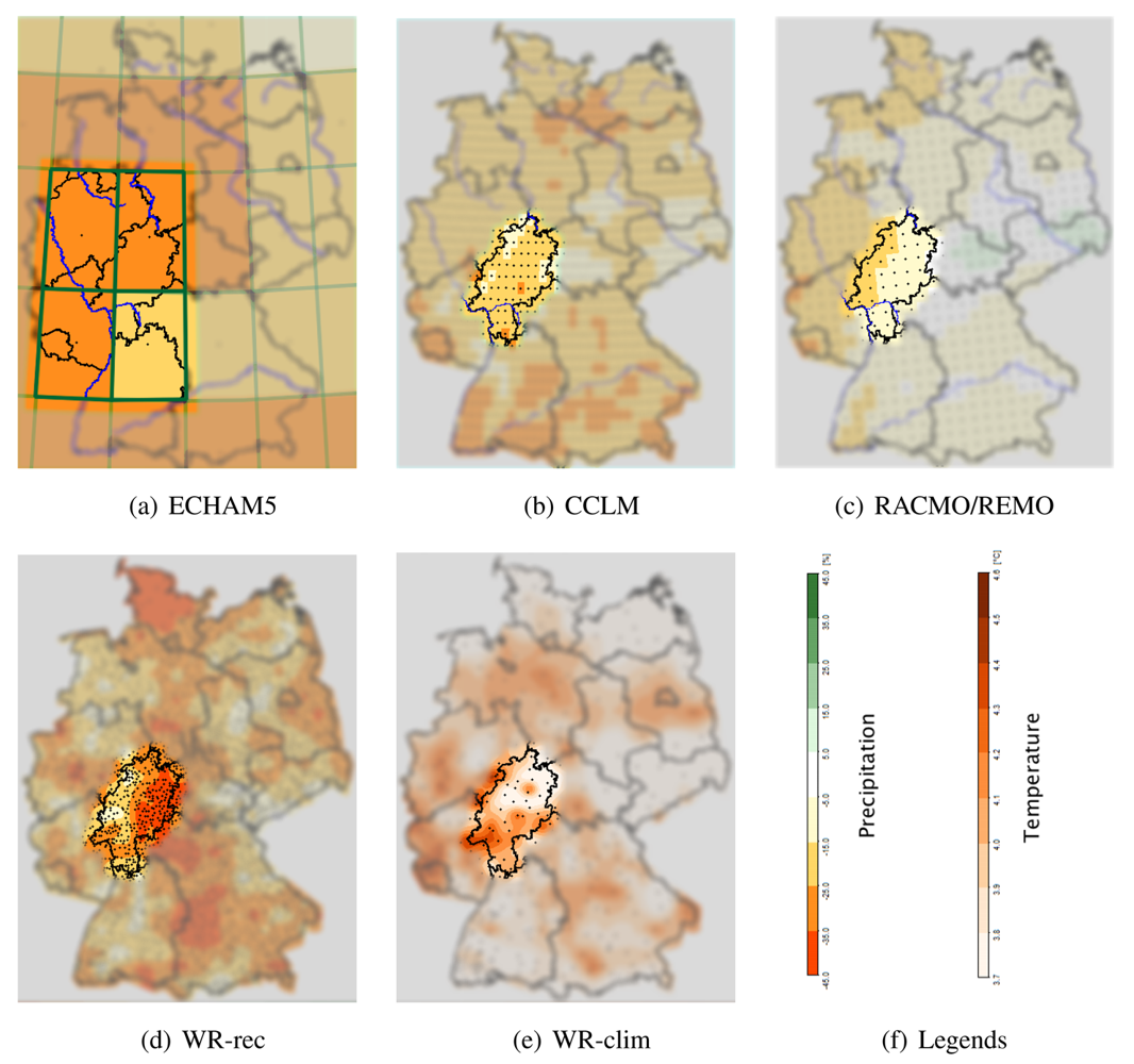
  • Surface measurements of meteorological elements (e.g., temperature, precipitation, humidity, cloudiness and wind). These were supplied by the German Weather Service and encompass 123 (35) climate stations and 908 (215) precipitation stations in the area around the Federal State of Hesse (number of stations within Hesse are denoted in parentheses). Figure 1(d) shows the density of the climate stations network and in Figure 1(e) the precipitation station network is shown—both for the highlighted area of the State of Hesse.

• Purpose: Direct study of a GCM as a basis for comparison with higher-resolution RCMs forced by the GCM as well as comparisons of the model cascades GCM > ESD with GCM > RCM

  • Results from a combination of the ECHAM5 atmosphere model with the ocean model OM1; this is the version of the ECHAM-model used in the 4th Assessment Report of the IPCC. This particular atmosphere-ocean model combination is frequently referred to as ECHAM5 [23]. It is applied for both, the reconstruction of the current climate (so-called 20C runs) and scenarios (runs 1, 2 and 3 of A1B) of the 21st century. (Source http://cera-www.dkrz.de). Figure 1(a) shows the density of the ECHAM5 grid over Germany.

• Purpose: Direct study of an RCM as well as comparison of model cascades GCM > WETTREG and GCM > RCM > WETTREG

  • Stream 3 results from the COSMO-CLM (CCLM) model [24], an RCM in its version 2.4.11. The CCLM runs were carried out by the group Models & Data at the Max Planck Institute for Meteorology in Hamburg in close co-operation with the developers of CCLM: Brandenburgian Technical University Cottbus (BTU), GKSS Research Centre Geesthacht and Potsdam Institute for Climate Impact Research (PIK). Funding was provided by the German Ministry of Education and Research (BMBF) in the framework of the support focus “klimazwei”. (source http://cera-www.dkrz.de). The study two uses CCLM runs based on SRES A1B ECHAM5 run 1 and run 2, respectively. Figure 1(b) shows the density of the CCLM grid over Germany.

  • Results from the REMO model [25], an RCM, the version 5.7 of which is described in [26]. (Source http://ensemblesrt3.dmi.dk). These REMO data are based on SRES A1B ECHAM5 run 3. Figure 1(c) shows the density of the RACMO grid over Germany which is identical to the REMO grid.

  • Results from the RACMO (RAC) model [27], an RCM in its version 2.1. (Source http://ensemblesrt3.dmi.dk). These RACMO data are based on SRES A1B ECHAM5 run 3. Figure 1(c) shows the density of the RACMO grid over Germany.

3. Method

3.1. Numerical Models Used

As can be seen from the items listed in Section 2 there is a manageable number of models employed in this study. The number of permutations can easily run out of hand if, e.g., several GCMs would be used. Therefore “only” ECHAM5/OM1 is the large scale model of choice. The bandwidth of GCM/RCM combinations is well represented by ECHAM5/OM1 runs driving CLM (two runs), REMO and RACMO.

3.2. The Empirical Statistical Downscaling Method WETTREG

WETTREG (weather situation-based regression method—in German: WETTerlagen-basierte REGressionsmethode) is an empirical statistical downscaling method that links large-scale features of the atmosphere to locally measured climate. It has been described in [28] and [29] Subsections 3.1 through 3.3. In a nutshell, WETTREG assumes, along the lines of a Filipo Giorgi quote in [30] that GCMs merit to be used as vantage ground for downscaling, since, owing to their ability to produce climate change patterns in a consistent way, they constitute a meaningful tool for obtaining local information from global patterns. Translated into terms of statistical climatology this means that changes over time of a parameter measured at the surface should coincide with changes of the occurrence frequency of large scale atmospheric patterns. This is the key to WETTREG where the regionalization is addressed in three stages:

• Patterns are defined using the environment-to-circulation strategy [31] in which intervals of a measured climate parameter (e.g., temperature) are specified and subsequently composites of the atmospheric situations on those days belonging to a temperature interval are built. This set of patterns, developed as a linkage between local time series and reanalysis data, are the building blocks for a subsequent objective re-identification procedure in the data of a climate model–details on these aspects can be found in [29,32]. The authors of [18,33] refer to the importance of choosing optimal predictors—this is taken into account within WETTREG by using relative topography fields for the temperature-related patterns and vorticity fields for the precipitation-related patterns. What emerges from this stage is a frequency distribution of the patterns [34] that shifts over time. In principle, it should be possible to apply the re-identification to GCM or RCM results (20C as well as scenario runs)—it is one of the core aspects of this study to compare and analyze the effect of using different sources.

• A stochastical weather generator is employed. It randomly re-arranges episodes from the current climate, of which the frequency of the patterns is known, into new, synthesized time series. The signature of the changing climate is grafted onto these synthesized series by the requirement that the (shifted) frequency of the patterns for a specific future time frame is a feature of the synthesized time series. Consequently some episodes appear more frequently than others.

• As a further refinement, the large-scale models are consulted again, and changes over time in the modeled physical properties of the atmosphere are introduced to the synthesized time series by way of regression.

The result of applying WETTREG is a set of time series at the location of climate stations which bear the signature of a shifting climate. Furthermore, there are ten simulations produced which are equally probable and constitute variants of the projected climate.

The WETTREG method as it was described in [28,29] had in the meantime been subjected to a few modifications, sketched in [35]—more comprehensive information (in German) can be found in [36,37], leading to the version WETTREG2010. For one, there was a transition in the property upon which the environment-to-circulation approach builds its classification—in WETTREG2010 it is the deviation from the annual cycle instead of the value itself. For two, additional weather situations, so-called Trans Weather Patterns, were introduced that emerge in the future and cannot be inferred from statistics of the current climate. The net effect is a greater proximity of the climate signals, in particular with respect to temperature, in regionalized WETTREG2010 projections to those produced by GCMs and GCM/RCM combinations.

WETTREG is conditioned to reproduce the climate of 1971–2000 with an accuracy of ±0.1° K (2 m mean temperature) and ±5% (precipitation) for each season. GCMs and RCMs are known to have systematic biases when reproducing this time frame. The issue of bias is covered, e.g., in [38] or [39] but will not be dealt with in this paper.

3.3. Evaluation Strategy

Climate signals are computed as areal means over the State of Hesse. The evaluated property is the difference of the 20C values for the period 1971–2000 and the A1B scenario data for the periods 2021–2050 and 2071–2100. The evaluation area is the entire State of Hesse. The authors acknowledge that an RCM with its high density of information as well as the station grid on which the information is produced by WETTREG (regardless of the actual version used), deliver different amounts of local detail. Yet, for inter-comparison purposes from GCM and RCM sources, the areal average is a more suitable measure.

Concerning the input data, four types need to be distinguished and are referred to using the abbreviations below. Since the GCM is the first stage of all cascades in 2–4 below, it is omitted from the nomenclature.

• Direct model output (DMO)—using the regional results straight from ECHAM5, evaluated at the four grid points in the State of Hesse, as shown in Figure 1 (a).

• Cascade GCM-RCM (CCLM, RAC and REMO)—using an RCM nested into a GCM, evaluated at an RCM-dependent number of grid points in the State of Hesse.

• Cascade GCM-ESD (WR)—using the GCM in its pattern-building capacity (cf. Subsection 3.2).

• Cascade GCM-RCM-ESD (CCLM > WR, RAC > WR and REMO > WR)—using the respective RCM in its pattern-building capacity (cf. Subsection 3.2).

When analyzing the variability of the climate for 30-year periods season-wise (not part of this study) it turns out that deviations leave the envelope of the climate “noise”—and thus can be interpreted as a climate signal—when they are larger than ±0.3° K (2 m mean temperature) or ±10% (precipitation).

Please note that for cascades of type 4, above, the RCM data had to be low pass filtered. As an experience from [20] the similarity search which WETTREG carried out in selected atmospheric fields is better suited to large scale patterns with not too fine detail.

4. Results

Regional signals from a global model? Due to their resolution, global models can only be of limited use for the assessment of regional climate signals [6]. This very fact is the main reason for the existence and progress of regionalization. The authors wish to underline that the results used from ECHAM5 directly (type 1 input, cf. Section 3.3) are but indicators for the magnitude of the climate signals. These are compared with projections which were obtained through regionalizations forced by the GCM.

4.1. Temperature Signals

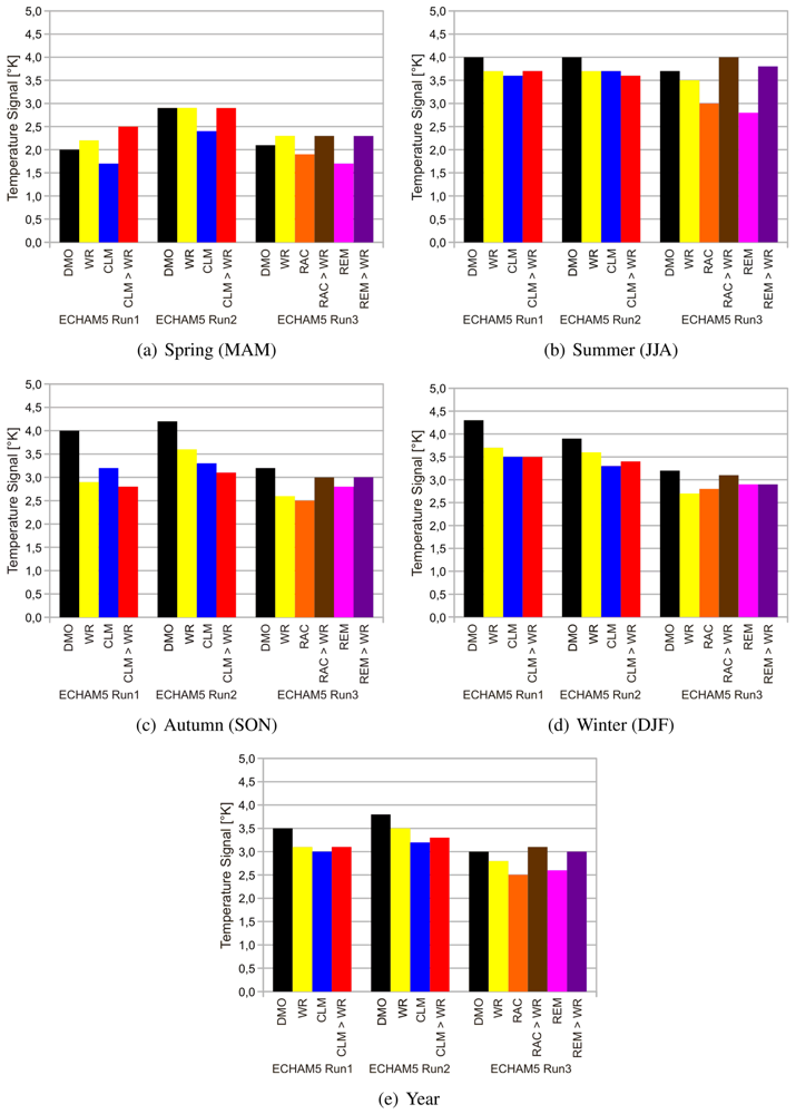
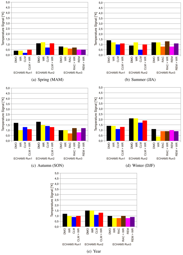
As shown in Figure 2 and 3 the temperature differences can be termed signals, according to the threshold given in Section 3.3. They are of similar magnitude for each season and across the different cascade types. This is an important outcome of the study. The variations that can be seen are, e.g., model run-specific. The bars in the graphs are arranged so that respective groups for each of the three ECHAM5 runs are formed. The signals that were extracted directly from ECHAM5 without any downscaling (DMO, black bar in every group) and are used as indicators for the signal magnitude tend to be among the highest. A regionalization with WETTREG (yellow bars) frequently yields lower temperature signals than the DMO results, yet they are frequently the strongest of the different cascade types forced by a specific ECHAM5 run.

Looking at seasonal features, it should be noted, and is known from numerous studies, that the signal in the spring temperature is lower than in other seasons. This appears to be a specific “meta signal” of ECHAM5; it is well visible in the 2071–2100 projections but can be traced in the 2021–2050 period already.

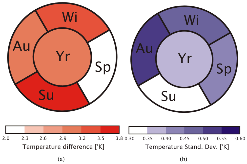
An overview of the seasonal behaviour of the temperature signal 2071–2100 minus 1971–2000 for all ensemble members (excluding DMO) is displayed in Figure 4. For one, the comparably small temperature increase in spring stands out in Figure 4(a) and for two the standard deviation, which can be interpreted as the a measure of “disagreement” between the models, shows that summer conditions are most coherently projected, whereas in autumn and winter the inter-model variability appears to be larger.

The type of cascade is a further cause of variation in the magnitude of the determined temperature signal. There are numerous examples for results from a type 4 (GCM > RCM > ESD) cascade being higher than from a type 2 (GCM > RCM) cascade, especially for combinations involving RACMO (orange and brown columns) or REMO (magenta and lilac columns) which are displayed in the right-hand groups of bars in Figures 2 and 3. This is most prominently exhibited in summer and autumn.

4.2. Precipitation Signals

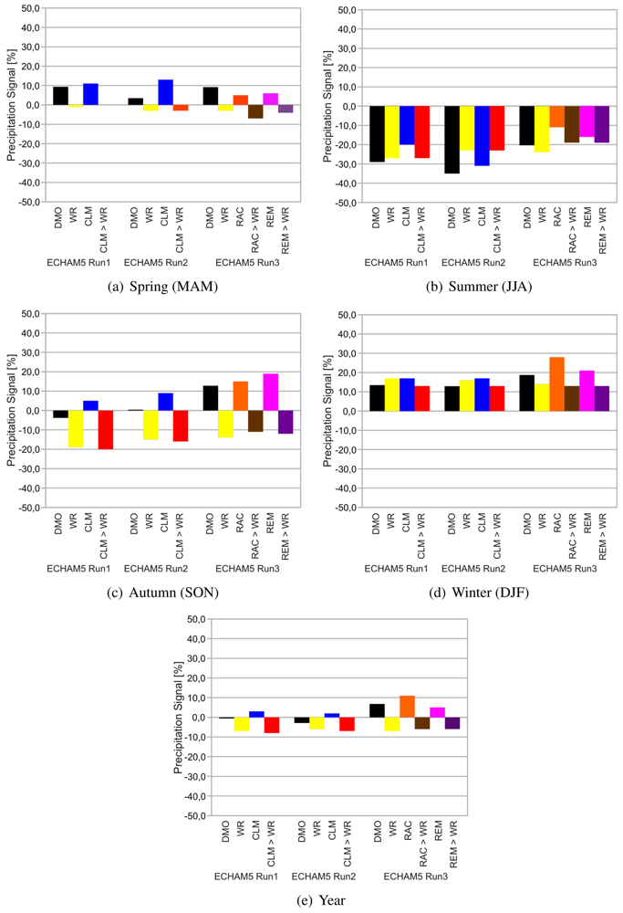
Clearly, the precipitation differences shown in Figures 5 and 6 frequently do not leave the value envelope indicated in Section 3.3 which would make them distinguishable from noise. This is in particular the case for the 2021–2050 data where 10%–15% is barely reached by a few model projections. For the period 2071–2100 the percentual precipitation changes in summer, autumn and winter is comparably often in the 20%–40% range.

Concerning the sign of the changes we find unambiguous conditions in summer and winter, i.e., evidence for an agreement on summer precipitation decrease and winter increase across all cascades and cascade types. For the transition seasons spring and autumn the picture is more complex. Type 3 and type 4 cascades that involve WETTREG yield a slight to medium decrease—more clearly developed in the 2071–2100 projections than in those for 2021–2050—and type 2 cascades exhibit a slight increase.

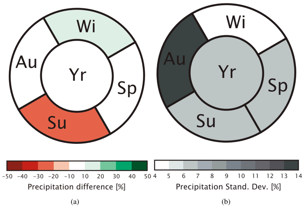
The ring diagrams (Figure 7) of mean (left) and standard deviation (right) of the precipitation signals 2071–2100 minus 1971–2000 underline that the two-fold development in the projected future climate (increase in winter and decrease in summer, Figure 7(a)) is captured by the entire ensemble (leaving out the DMO results—yet if they would be inserted this would only make a minor difference). Moreover, the particular autumn conditions stick out in Figure 7(b) where the comparably large “disagreement” between the ensemble members can be seen.

5. Conclusions and Outlook

A study was carried out that addresses the issue of the sensitivity of climate signals with respect to the regionalization strategy employed. It uses one GCM (ECHAM5) in two roles: (i) as an indicator for the magnitude of the regional climate signals and (ii) as the forcing model for dynamical and empirical statistical downscaling. An ensemble was drafted which encompasses two-tier model cascades (GCM > RCM as well as GCM > ESD) and three-tier cascades, i.e., GCM > RCM > ESD. The project design is based on the knowledge that the higher resolved orography of RCMs influences the storm tracks and the local weather. The representation of the Alps, e.g., is crucial for local weather in Germany.

The three RCMs forced by ECHAM5 are CCLM (ECHAM5 runs 1 and 2), REMO and RACMO (both with ECHAM5 run 3). WETTREG is the statistical method forced by either ECHAM5 (all three runs) or one of the aforementioned RCMs. The target area is the German Federal State of Hesse and the material that has been analyzed and interpreted consists of the differences between 20C results (period 1971–2000) and A1B scenario runs (periods 2021–2050 and 2071–2100) for ECHAM5 and the various cascades in the ensemble.

Concerning daily average temperature an important outcome is that there is an overall similarity in signal magnitude between the GCM and the different cascade results. The fact that, despite the methodological differences between the downscaling approaches, there is an indication of agreement adds confidence in the robustness of the climate signals. Using the signals from the GCM projection as a reference there is a tendency that the projections by the downscaling cascades are below the GCM results. The magnitude of the temperature signal is comparably low in spring (2–3 °K temperature increase for projections into the 2071–2100 period) with respect to the other seasons (2.5–4 °K increase). There is evidence that, at least when involving REMO or RACMO, there is a distinction between two-tier and three-tier cascades. A regionalization with WETTREG yields clearly higher signals than one without, best visible in spring and summer.

Concerning precipitation it is noteworthy that changes between the periods 1971–2000 (20C) and 2021–2050 (scenario A1B) stay within the bounds of noise and that changes with respect to 2071–2100 for all seasons except spring do constitute a signal. For the 2071–2100 period and for the transition seasons autumn and (to a smaller degree) spring, an inverse behaviour was detected between the cascades that involve WETTREG (either as two-tier or as three-tier types) where slightly negative signals prevail and the two-tier cascades involving any of the RCMs where weak to moderate positive signals were detected. The summer precipitation signals are clearly indicating a reduction between 10% and 35% and no obvious distinction between the signal magnitudes projected by the different cascade types. Winter signals indicate a precipitation increase between 10% and 25% across all cascades with a tendency of three-tier cascades yielding slightly smaller signals than any two-tier cascade.

Thus it can be concluded that there is evidence for a dependency of the regional temperature and precipitation signal on the pathway with which a downscaling is arrived at. However, an attribution to that pathway is complex since the signals also depend on the RCM used and the run of the forcing GCM. In the current version of WETTREG the differences between both cascades are small. This may be due to the fact that there are only small differences in the large scale circulation between the forcing GCM and the RCM. Or the transfer functions used in WETTREG are not sensible enough for differences of such a small magnitude.

In this stage of our research, the focus was the analysis of an ensemble of different downscaling strategies and the detection of particularities that indicate a connection to the type of downscaling strategy employed. Future investigation will have to be carried out, e.g., concerning reasons why the precipitation signal in the transition seasons has such a distinct behaviour.

References and Notes

- Kerr, R. Climate change-Three degrees of consensus. Science 2004, 305, 932–934. [Google Scholar]
- IPCC. Climate Change. The IPCC Scientific Assessment. Intergovernmental Panel on Climate Change; Cambridge University Press: Cambridge, UK, 1990. [Google Scholar]
- IPCC. Climate Change 1995. The Science of Climate Change. Contribution of Working Group I to the Second Assessment Report of the Intergovernmental Panel on Climate Change; Cambridge University Press: Cambridge, UK, 1996. [Google Scholar]
- IPCC. Climate Change 2001: The Scientific Basis; Contribution of Working Group I to the Third Assessment Report of the Intergovernmental Panel on Climate Change; Cambridge University Press: Cambridge, UK, 2001. [Google Scholar]
- IPCC. Climate Change 2007: The Physical Science Basis. Contribution of Working Group I to the Fourth Assessment Report of the Intergovernmental Panel on Climate Change; ISBN: Number ISBN: 978 0521 70596-7. Cambridge University Press: Cambridge, UK and New York, USA, 2007. [Google Scholar]
- Grotch, S.; MacCracken, M. The use of general circulation models to predict regional climatic change. J. Climate 1991, 4, 286–303. [Google Scholar]
- IPCC. The Regional Impacts of Climate Change-An Assessment of Vulnerability; Cambridge University Press: Cambridge, UK, 1998. [Google Scholar]
- Dickinson, R.; Enrico, R.; Giorgi, F.; Bates, G. A regional climate model for the western U.S. Climatic Change 1989, 15, 383–422. [Google Scholar]
- Giorgi, F. Simulation of regional climate using a limited area model nested in a general circulation model. J. Climate 1990, 3, 941–963. [Google Scholar]
- Giorgi, F.; Mearns, L. Approaches to the simulations of regional climate change: A review. Rev. Geophys. Space Phys. 1991, 29, 191–216. [Google Scholar]
- Wilby, R.; Wigley, T. Downscaling general circulation model output: A review of methods and limitations. Progr. Phys. Geogr. 1997, 21, 530–548. [Google Scholar]
- Huth, R. Statistical downscaling in central Europe: Evaluation of methods and potential predictors. Clim. Res. 1999, 13, 91–101. [Google Scholar]
- Cess, R.; Potter, G.; Blanchet, J.; Boer, G.; Ghan, S.; Kiehl, J.; Le Treut, H.; Liang, X.; Mitchell, J.; Morcrette, J.; et al. Interpretation of cloud-climate feedback as produced by 14 atmospheric general circulation models. Science 1989, 245, 513–516. [Google Scholar]
- Meehl, G.; Boer, G.; Covey, C.; Latif, M.; Stouffer, R. The coupled model intercomparison project (CMIP). Bull. Am. Meteorol. Soc. 2000, 81, 313–318. [Google Scholar]
- Christensen, J.H. Prediction of Regional Scenarios and Uncertainties for Defining European Climate Change Risks and Effects, Final Report; (PRUDENCE); Technical Report; Danish Meteorological Institut (DMI): Copenhagen, Denmark, 2005. [Google Scholar]
- Christensen, J.; Carter, T.; Rummukainen, M.; Amanatidis, G. Evaluating the performance and utility of regional climate models: The PRUDENCE project. Climatic Change 2007, 81, 1–6. [Google Scholar]
- Hanson, C.; Palutikof, J.; Livermore, M.; Barring, L.; Bindi, M.; Corte-Real, J.; Durao, R.; Giannakopoulos, C.; Good, P.; Holt, T.; et al. Modelling the impact of climate extremes: An overview of the MICE project. Climatic Change 2007, 81, 163–177. [Google Scholar]
- Goodess, C.; STARDEX. Downscaling Climate Extremes, Final Report; Technical Report; STARDEX Consortium: Norwich, UK, 2009. [Google Scholar]
- Van der Linden, P.; Mitchell, J. ENSEMBLES: Climate Change and Its Impacts: Summary of Research and Results from the ENSEMBLES Project; Met Office Hadley Centre: FitzRoy Road, Exeter EX1 3PB, UK, 2009. [Google Scholar]
- Kreienkamp, F.; Spekat, A.; Enke, W. Sensitivity studies with a statistical downscaling method—the role of the driving large scale model. Meteorol. Z. 2009, 18, 597–606. [Google Scholar]
- Kalnay, E.; Kanamitsu, M.; Kistler, R.; Collins, W.; Deaven, D.; Gandin, L.; Iredell, M.; Saha, S.; Whitea, G.; Woolen, J.; et al. The NCEP/NCAR 40-year reanalysis project. Bull. Am. Meteorol. Soc. 1996, 77, 437–471. [Google Scholar]
- Uppala, S.; Kållberg, P.; Simmons, A.; Andrae, U.; da Costa Bechtold, V.; Fiorino, M.; Gibson, J.; Haseler, J.; Hernandez, A.; Kelly, G.; et al. The ERA-40 re-analysis. Quart. J. Roy. Meteorol. Soc. 2005, 131, 2961–3012. [Google Scholar]
- Roeckner, E.; Baeuml, G.; Bonaventura, L.; Brokopf, R.; Esch, M.; Giorgetta, M.; Hagemann, S.; Kirchner, I.; Kornblueh, L.; Manzini, E.; et al. The Atmospheric General Circulation Model ECHAM5-Part 1: Model Description; Max Planck Institut for Meteorology: Hamburg, Germany; November; 2003. [Google Scholar]
- Böhm, U.; Kücken, M.; Ahrens, W.; Block, A.; Hauffe, D.; Keuler, D.; Rockel, B.; Will, A. CLM–The Climate Version of LM: Brief description and long-term applications. COSMO Newslett. 2006, 6, 225–235. [Google Scholar]
- Jacob, D.; Podzun, R. Sensitivity studies with the regional climate model REMO. Meteorol. Atmos. Phys. 1997, 63, 119–129. [Google Scholar]
- Jacob, D.; Göttel, H.; Kotlarski, S.; Lorenz, P.; Sieck, K. Klimaauswirkungen und Anpassung in Deutschland-Phase 1: Erstellung regionaler Klimaszenarien für Deutschland; Technical Report; Max-Planck-Institut für Meteorologie (MPI-M): Hamburg, Germany, 2008. [Google Scholar]
- Lenderink, G.; van den Hurk, B.; van Meijgaard, E.; van Ulden, A.; Cuijpers, J. Simulation of Present-Day Climate in RACMO2: First Results and Model Developments; Technical Report; Koninklijk Nederlaidse Meteolognsch Instituut: Tilburg, The Netherlands, 2003. [Google Scholar]
- Enke, W.; Deutschländer, T.; Schneider, F.; Küchler, W. Results of five regional climate studies applying a weather patter based downscaling method to ECHAM4 climate simulations. Meteorol. Z. 2005, 14, 247–257. [Google Scholar]
- Spekat, A.; Kreienkamp, F.; Enke, W. An impact-oriented classification method for atmospheric patterns. Phys. Chem. Earth 2010, 35, 352–359. [Google Scholar]
- Schiermeier, Q. High-resolution climate modelling: Assessment, added value and applications. Nature 2004, 428, 593. [Google Scholar]
- Yarnal, B. Synoptic Climatology in Environmental Analysis; Belhaven Press: London, UK, 1993. [Google Scholar]
- Enke, W.; Schneider, F.; Deutschländer, T. A novel scheme to derive optimized circulation pattern classifications for downscaling and forecast purposes. Theor. Appl. Climatol. 2005, 82, 51–63. [Google Scholar]
- Timbal, B.; Hope, P.; Charles, S. Evaluating the consistency between statistically downscaled and global dynamical model climate change projections. J. Climate 2008, 21, 6052–6059. [Google Scholar]
- Using temperature again as an illustration, the patterns are arranged in ascending order from those that linked to low surface temperature (the “cold” patterns) to those that are linked to high temperature (the “warm” patterns). “Dry” and “wet” patterns would be the analogues in the humidity regime.
- Kreienkamp, F.; Spekat, A.; Enke, W. TransWeather Patterns—an extended outlook for the future climate. EMS Annual Meeting Abstracts 2010, 7, 2010–2453. [Google Scholar]
- Kreienkamp, F.; Spekat, A.; Enke, W. Weiterentwicklung von WETTREG bezüglich neuartiger Wetterlagen, Technical Report (in German); Available online: http://klimawandel.hlug.de/fileadmin/dokumente/kilma/inklim_a/TWL_Laender.pdf (accessed on 20 May 2011).
- Kreienkamp, F.; Spekat, A.; Enke, W. Ergebnisse eines regionalen Szenarienlaufs für Deutschland mit dem statistischen Modell WETTREG2010; Technical Report; Climate and Environment Consulting Potsdam GmbH on a contract of the Federal Environment Agency (UBA): Potsdam, Dessau, Germany, 2010. [Google Scholar]
- Christensen, J.; Boberg, F.; Christensen, O.; Lucas-Picher, P. On the need for bias correction of regional climate change projections of temperature and precipitation. Geophys. Res. Lett. 2008, 35, 1–6. [Google Scholar]
- Maraun, D.; Wetterhall, F.; Ireson, A.; Chandler, R.; Kendon, E.; Widmann, M.; Brienen, S.; Rust, H.; Sauter, T.; Themeßl, M.; et al. Precipitation downscaling under climate change. Recent developments to bridge the gap between dynamical models and the end user. Rev. Geophys. 2010, 48, 1–34. [Google Scholar]
© 2011 by the authors; licensee MDPI, Basel, Switzerland. This article is an open access article distributed under the terms and conditions of the Creative Commons Attribution license (http://creativecommons.org/licenses/by/3.0/.)
Share and Cite
Kreienkamp, F.; Baumgart, S.; Spekat, A.; Enke, W. Climate Signals on the Regional Scale Derived with a Statistical Method: Relevance of the Driving Model’s Resolution. Atmosphere 2011, 2, 129-145. https://doi.org/10.3390/atmos2020129
Kreienkamp F, Baumgart S, Spekat A, Enke W. Climate Signals on the Regional Scale Derived with a Statistical Method: Relevance of the Driving Model’s Resolution. Atmosphere. 2011; 2(2):129-145. https://doi.org/10.3390/atmos2020129
Chicago/Turabian StyleKreienkamp, Frank, Sonja Baumgart, Arne Spekat, and Wolfgang Enke. 2011. "Climate Signals on the Regional Scale Derived with a Statistical Method: Relevance of the Driving Model’s Resolution" Atmosphere 2, no. 2: 129-145. https://doi.org/10.3390/atmos2020129