Influence of Climatic Changes on Pollution Levels in Hungary and Surrounding Countries

Abstract
: The influence of future climatic changes on some high pollution levels that can cause damage to plants and human beings is studied in this paper. The particular area of interest is Hungary and its surrounding countries. Three important quantities, which are closely related to ozone concentrations, have been investigated. We shall mainly focus on cases where the critical values, prescribed in the directives, are exceeded. Six scenarios, which allow us to compare directly the future and the present levels, have been run over a period of sixteen years. Some of the results obtained in the selected domain by using these scenarios have been carefully studied. The major conclusion is that an increase in temperature in combination with some other factors might lead to rather considerable increases of the damaging effects of ozone on plants and humans.1. Introduction
The gradual increase of temperature is the major effect of predicted climatic change. In fact, most of the other climatic changes are merely consequences of the increased temperature. Therefore, it is important to study the impact of the increasing temperatures on the pollution levels in different areas of the Earth. It is clear that the pollution levels will be sensitive to the increase of the temperature, because both the biogenic emissions and many of the chemical reactions depend on the temperature. It is more important, however, to evaluate the magnitude of the changes of some pollution levels that are caused by the higher temperatures. Some aspects of the influence of climate changes on the pollution levels in some parts of Europe have been treated in several papers recently; see, for example [1] and [2] as well as some of the references given in these two papers.
The influence of climate changes (and, first and foremost, the influence of the increased temperature) on the pollution levels in Hungary is the major topic of this paper. However, better understanding of the studied phenomena can only be achieved when two additional issues are also investigated:
the impact of the climate changes on the pollution levels in the countries that are located near to Hungary;
and
the changes of the pollution levels that are due to a combination of the warming effect with some other important factors.
In connection with requirement (a), the studied model domain will contain not only Hungary, but also its neighboring countries.
In connection with requirement (b), it was important to compare the changes of the pollution levels in the studied area that are caused by future increases of the temperature with the changes that are created by several other factors (different emissions, inter-annual variability of meteorological conditions, etc.). Such an extensive comparison has successfully been accomplished by designing several different scenarios.
Three important quantities, which are closely related to ozone concentrations, have been studied:
AOT40C, i.e., accumulated over a threshold of 40 ppb ozone concentrations for crops (high AOT40C values can cause damage to plants and, first and foremost, crops),
AOT40F, i.e., accumulated over a threshold of 40 ppb ozone concentrations for forests (high AOT40F values can cause damage to forest trees),
Number of “bad days” (large numbers of “bad days” can cause damage to people suffering from asthmatic diseases).
Critical levels for these three quantities are given in several directives of the European Parliament (see [3]: Directive 2002/3/EC of the European Parliament and the Council of 12 February 2002 relating to ozone in ambient air. Official Journal of the European Communities, L67, 9.3.2002, pp. 14-30).
The total number of the scenarios was fourteen. In this study we only present the results obtained from six selected scenarios, but the description of the other eight scenarios can be found in [7]. It was necessary to run all these scenarios over a long time period, i.e. 16 years, to capture both climatic and inter-annual variations.
This paper is organized in the following way:
The particular model used, the Unified Danish Eulerian Model (UNI-DEM), is briefly described in Section 2.
The six scenarios that are applied in the investigations are defined in Section 3.
Results obtained in connection with AOT40C values are presented and discussed in Section 4.
Results obtained in connection with AOT40F values are presented and discussed in Section 5.
Results obtained in connection with “bad days” are presented and discussed in Section 6.
General conclusions and remarks are given in the last section.
2. Mathematical Description of an Environmental Model
UNI-DEM (the Unified Danish Eulerian Model) is a large air pollution model for studying the long-range transport of air pollutants in the atmosphere. The space domain of the model contains the whole of Europe with some parts of Asia, Africa and the Atlantic Ocean. All important physical processes (advection, diffusion, deposition, emissions and chemical reactions) are represented in the mathematical formulation of the model. All important chemical species (sulfur pollutants, nitrogen pollutants, ammonia-ammonium, ozone, as well as many radicals and hydrocarbons) can be studied by the model. The chemical reactions are described by using the well-known condensed CBM IV scheme. The space domain is discretized by using (32 × 32), (96 × 96), (288 × 288) or (480 × 480) grid in the two-dimensional version of the model and (96 × 96 × 10), (288 × 288 × 10) or (480 × 480 × 10) grid in the three-dimensional version. The horizontal discretization is performed by using equidistant grid squares of the size (150 km × 150 km), (50 km × 50 km), (16.7 km × 16.7 km) or (10 km × 10 km), while non-equidistant grid is used in the vertical direction (with finer resolution close to the surface).
UNI-DEM (the Unified Danish Eulerian Model) is, as many other environmental models, described mathematically by a system of q partial differential equations (PDEs):
ci = ci (t, x, y, z) is the concentration of the chemical species i at point (x, y, z) of the space domain and at time t of the time interval,
u = u(t, x, y, z), v = v(t, x, y, z) and w = w(t, x, y, z) are wind velocities along the Ox, Oy and Oz directions, respectively at point (x, y, z) and time t,
Kx = Kx (t, x, y, z), Ky = Ky (t, x, y, z) and Kz = Kz(t, x, y, z) are diffusivity coefficients at point (x, y, z) and time t (it is often assumed that Kx and Ky are non-negative constants, while the calculation of Kz is normally rather complicated),
k1i = k1i (t, x, y, z) and k2i = k2i (t, x, y, z) are deposition coefficients (dry and wet deposition respectively) of chemical species i at point (x, y, z) and time t of the time interval (for some of the species these coefficients are non-negative constants, the wet deposition coefficients k2i are equal to zero when it is not raining).
Normally it is not possible to solve exactly the systems of PDEs by which the large environmental models are described mathematically. Therefore, numerical methods must be used to find approximate values of the solution at the grid points defined on the domain of the model. It is also appropriate to split the model, the system of PDEs of type (1), into several sub-models (sub-systems), which are in some sense simpler. There is another advantage when some splitting procedure is applied: the different sub-systems have different properties and one can try to select the best numerical method for each of the sub-systems.
The discretization of the system of PDEs by which the environmental models are described mathematically leads to huge computational tasks. The following example illustrates clearly the size of these tasks. Assume that
Nx = Ny = 480 (when a 4800 km × 4800 km domain covering Europe is considered, then this choice of the discretization parameters leads to 10 km × 10 km horizontal cells),
Nz = 10 (i.e., ten layers in the vertical direction are introduced and it should be noted that they are not equidistant) and
Ns = q = 56 (the chemical scheme contains 56 species).
Then the number of equations that are to be handled at each time step is (Nx + 1)(Ny + 1)(Nz + 1)Ns = 142 518 376. A run over a time period of one year with a time step size Δt = 2.5 seconds will result in Nt = 213 120 time steps. When studies related to climatic changes are to be carried out, it is necessary to run the models over a time period of many years. When the sensitivity of the model to the variation of some parameters is studied, many scenarios (up to several hundred) are to be run. This short analysis demonstrates the fact that the computational tasks arising when environmental studies are to be carried out by using large-scale models are enormous. Therefore, it is necessary:
to select fast but sufficiently accurate numerical methods and/or splitting procedures,
to exploit efficiently the cache memories of the available computer,
to parallelize the code
The particular numerical methods and splitting procedure used when the system of PDEs represents UNI-DEM are discussed in detail in [4] and [5]. Optimizing the code for parallel computations on high-speed computers is discussed in [6] and [5].
3. Developing a Set of Appropriate Scenarios
Six scenarios were used in this study and all were run over a time period of 16 years by using fine resolution (10 km by 10 km surface cells) on the whole space domain of the model. Only results obtained in the territories of Hungary and its surrounding countries will be used in this paper. The major characteristics of the scenarios are summarized in Table 1. The scenarios are discussed in detail in [7], [8] and [9].
3.1. Running the Six Scenarios
Running six scenarios over a time period of 16 years on a fine grid (480x480x10 cells) is an extremely demanding task even when modern computers are available. Therefore it can be successfully solved only if several requirements are simultaneously satisfied: (a) fast but also sufficiently accurate numerical methods are to be implemented in the model; (b) the cache memories of the available computers have to be efficiently utilized; (c) codes which can be run in parallel have to be developed and used; and (d) reliable and robust splitting procedures have to be implemented. The solution of sub-tasks (a)–(d) is discussed in detail in [6] and [5]. It must be emphasized here that it is impossible to handle the six scenarios over a time period of 16 years on the available super-computers if the sub-tasks (a)–(d) are not efficiently solved. Even when this was done, it took nearly a year to compute the data from all 1152 runs (6 scenarios × 16 years × 12 months) carried out in this study. This fact illustrates the great computational difficulties that are related to the investigation of various impacts of climatic changes on pollution levels. The storage requirements (large input and output files) are also enormous.
3.2. Basic Scenario
Meteorological and emission data for sixteen years (from 1989 to 2004) prepared partly by EMEP (European Monitoring and Evaluation Programme, see [14] and [15]) and partly in NERI (the National Environmental Research Institute at Aarhus University; see [16]) were applied in the Basic Scenario. This scenario was used: (a) to verify the model results by comparing model results with measurements; and (b) to study the sensitivity of the model results to different changes of several essential parameters (inter-annual meteorological conditions, anthropogenic emissions, biogenic emissions and climatic changes) by comparing the results obtained by the Basic Scenario with results obtained by other scenarios.
Comparisons of concentrations calculated by the Basic Scenario and measurements have been reported for
A previous version of UNI-DEM, run with the Basic Scenario, has also been used in some inter-comparisons of European large-scale air pollution models [28,29].
3.3. Constant Meteorology versus Constant Anthropogenic Emissions
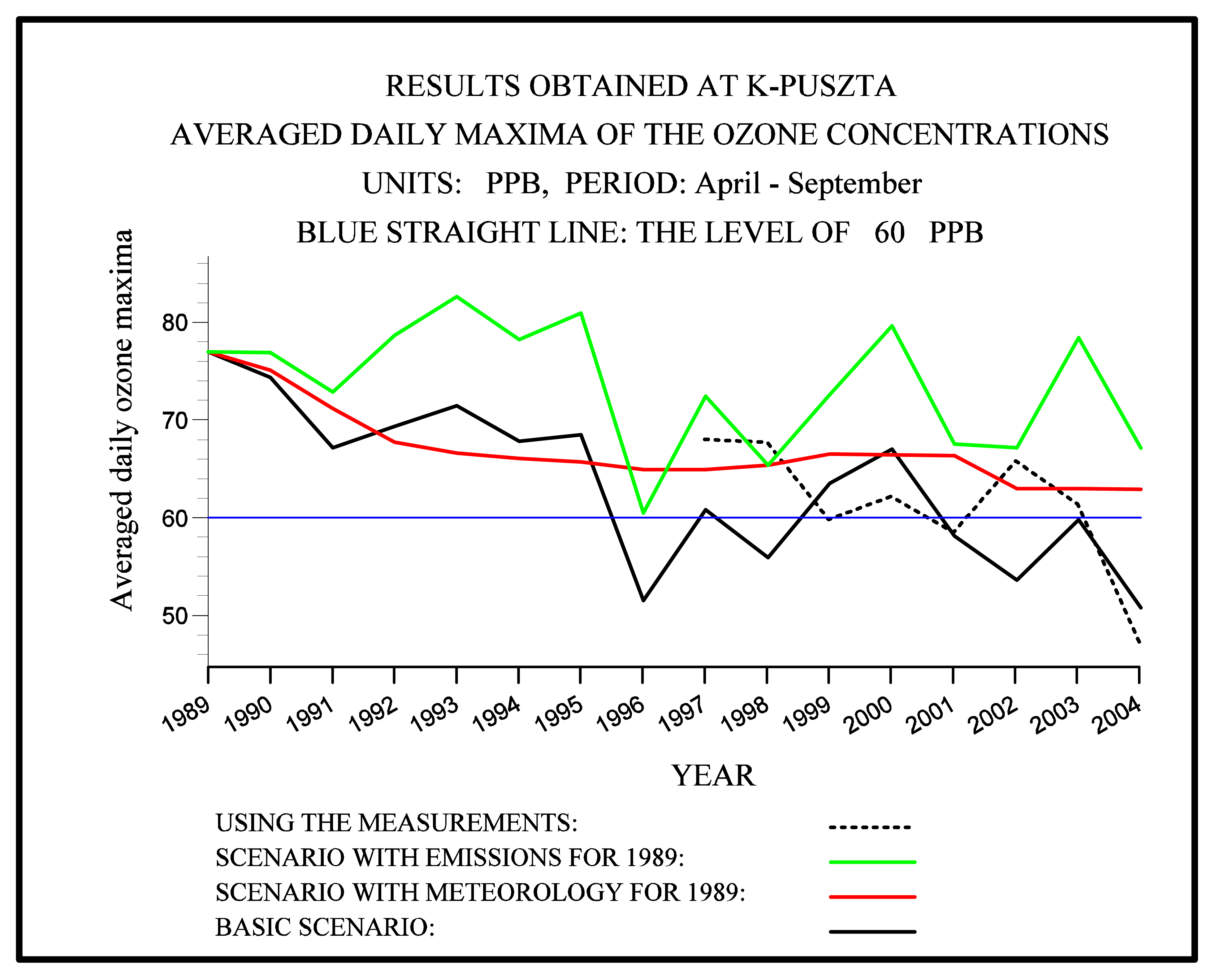
Two traditional scenarios were prepared and used. In the first scenario constant meteorology (the meteorological data for 1989) was used. In the second of these two scenarios the human-made (anthropogenic) emissions for 1989 were used during the whole period (from 1989 to 2004). Results obtained at the Hungarian measurement station K-puszta are given in Figure 1. Much more results can be found in [7].
When the first of these two scenarios, Scenario Constant Meteorology, is used, the trend showing reductions of the pollution levels is preserved, but the annual variability of the pollution levels disappears.
When the second scenario, Scenario Constant Emissions, is used, the annual variability of the pollution levels is preserved, but the trend showing reductions of the pollution levels disappears. The reductions of the European pollution levels are caused by the fact that the human-made (anthropogenic) emissions in Europe were reduced very considerably during the last two decades.
The main conclusion from the runs with these three scenarios is that it is necessary to carry out calculations over a long time period in order to be able to draw more useful and more reliable conclusions.
3.4. Climatic Scenario 3
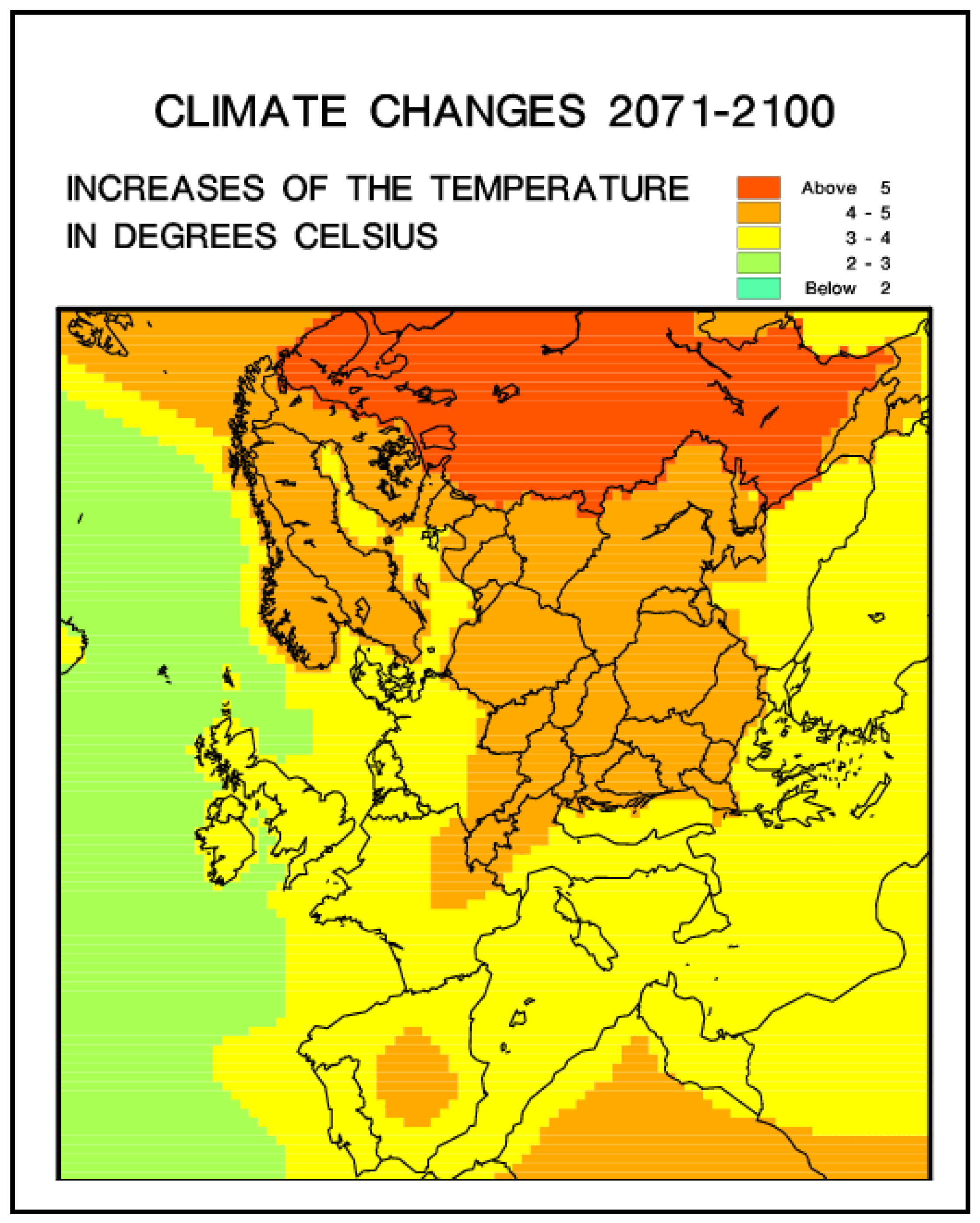
The major requirement for the climatic scenario was the following: we would like to easily compare the pollution levels predicted for the future with the present levels. It is difficult to satisfy this requirement by just running a climatic model. Assume that we did so and obtained (for some year in the future) that the average daily maximum would be, say, 60 ppb. Compare this number with the results shown in Figure 1. For some years it is less than the results obtained by the Basic Scenario (the black continuous curve in Figure 1), for other years it is greater. To be more precise, assume that we run our Basic Scenario for the period from 1989 to 2004 (as we actually did in the paper) and some climatic model for a period of the same length (say, from 2089 to 2104), consider the results for year 1996. The meteorological condition for the corresponding year 2096 will in general not be the same as those for 1996. If we want to compare the levels for 1996 with some corresponding levels calculated by the climatic model, then we have to find a year in which the meteorological conditions will be similar to those in 1996. This makes the comparison very difficult. No conclusion for some trends can be made (not easily at least). Therefore another approach must be used. We decided to keep the wind velocity fields the same as for the 16 years selected for this study and to increase the temperature as prescribed in the IPCC SRES A2 Scenario taking into account also some other climatic changes, which are discussed in [30] and [31]. Changes of the temperature in Europe, resulting from this scenario, are shown in Figure 2. Consider any cell of the grid used to create the plot shown in Figure 2 and assume that this cell is located in a region in Figure 2 where the increase of the temperature is in the interval [a,b]. The temperature at the chosen cell at a time n (where n is in the interval from 1989 to 2004) is increased by an amount a + c(n), where c(n) is randomly generated in the interval [0, b–a]. The mathematical expectation of the increase of the annual mean of the temperature at any cell of the space domain is (b–a)/2. In this manner, the mean value of the annual change of the temperature at a given point will tend to be the same as that prescribed by the IPCC SRES A2 Scenario for each year of the chosen interval (from 1989 to 2004).
The extreme cases will become even stronger in the future climate; see Table 9.6 on p. 575 in [30]; see also [31]. It is expected that:
there will be higher maximum temperatures and more hot days in the land areas,
there will be higher minimum temperatures, fewer cold days and fewer frost days in nearly all land areas, and
the diurnal temperature range will be reduced over land areas.
We increased the temperatures during the night with a factor larger than the factor by which the daytime temperatures were increased. In this way the second and the third requirements are satisfied. The first requirement is satisfied as follows. During the summer periods the daytime temperatures are increased by a larger amount in hot days. All these changes are carried out only over land. We also reduced the cloud covers over land during the summer periods.
It is also expected, see Table 9.6 on p. 575 in [30] and also [31] that:
there will be more intense precipitation events, and
there will be increased summer drying and an associated risk of drought.
We increased the precipitation events during winter (both over land and over water). During summer, the precipitation events in the continental parts of Europe were reduced. Similar changes in the humidity data were made. The cloud covers during winter were increased. The climatic scenario obtained in the above steps is referred to as Climatic Scenario 3 in [7], [8] and [9] and throughout this paper.
3.5. Emission Scenarios
Several scenarios in which the human-made (anthropogenic) emissions are varied were prepared and run in the period 1989–2004. In this study we used the MFR Scenario (MFR stands for “maximum feasible reductions”). This scenario is described and discussed in the IIASA report [32]. In this report (available from the Internet, see [33]) some factors related to Scenario 2010 are given for each country. The actual emissions for Scenario 2010 are obtained by multiplying the EMEP emissions for year 1990 by corresponding factors. Similar factors (but much smaller) are presented in the report for the MFR Scenario. Also the MFR Scenario is obtained by multiplying the EMEP emissions for year 1990 by corresponding factors. The relevant factors for this paper (the IIASA factors for the MFR Scenario and for the countries in the domain studied) are given in Table 2.
The reduction factors listed in [32] were used to obtain reduced emissions for this scenario and the scenario, obtained in this way, was run by using meteorological data for all years from 1989 to 2004. This means that the inter-annual variation of the meteorological conditions is preserved the same as in the Basic Scenario, while the emissions do not vary from one year to another.
The emissions obtained in this way and used in the MFR Scenario, were also used to derive an additional emission scenario, Scenario Climate MFR. This scenario was formed as a combination of the meteorological conditions derived from the Climate Scenario 3 and the predicted human-made (anthropogenic) emissions from Scenario MFR. The latter scenario was also run over the whole period from 1989 to 2004.
4. AOT40 Values for Crops
The AOT40 values for crops will be denoted as AOT40C and are related to ozone concentrations in the following way (more details can be found in [19]):
N is the number of day-time hours in the period May, June, July, and
ci is the ozone concentration (measured at a given station or calculated by a model at a given grid square) at hour i, where i∈{1, 2,…,N}.
If AOT40C exceeds 3000 ppb.hours, then this fact may lead to losses from crops for the area where this critical level is exceeded. This is why it is desirable to prevent the situation where the AOT40C values exceed 3000 ppb.hour. This is emphasized in several official documents of the European Union (EU); see, for example [3].
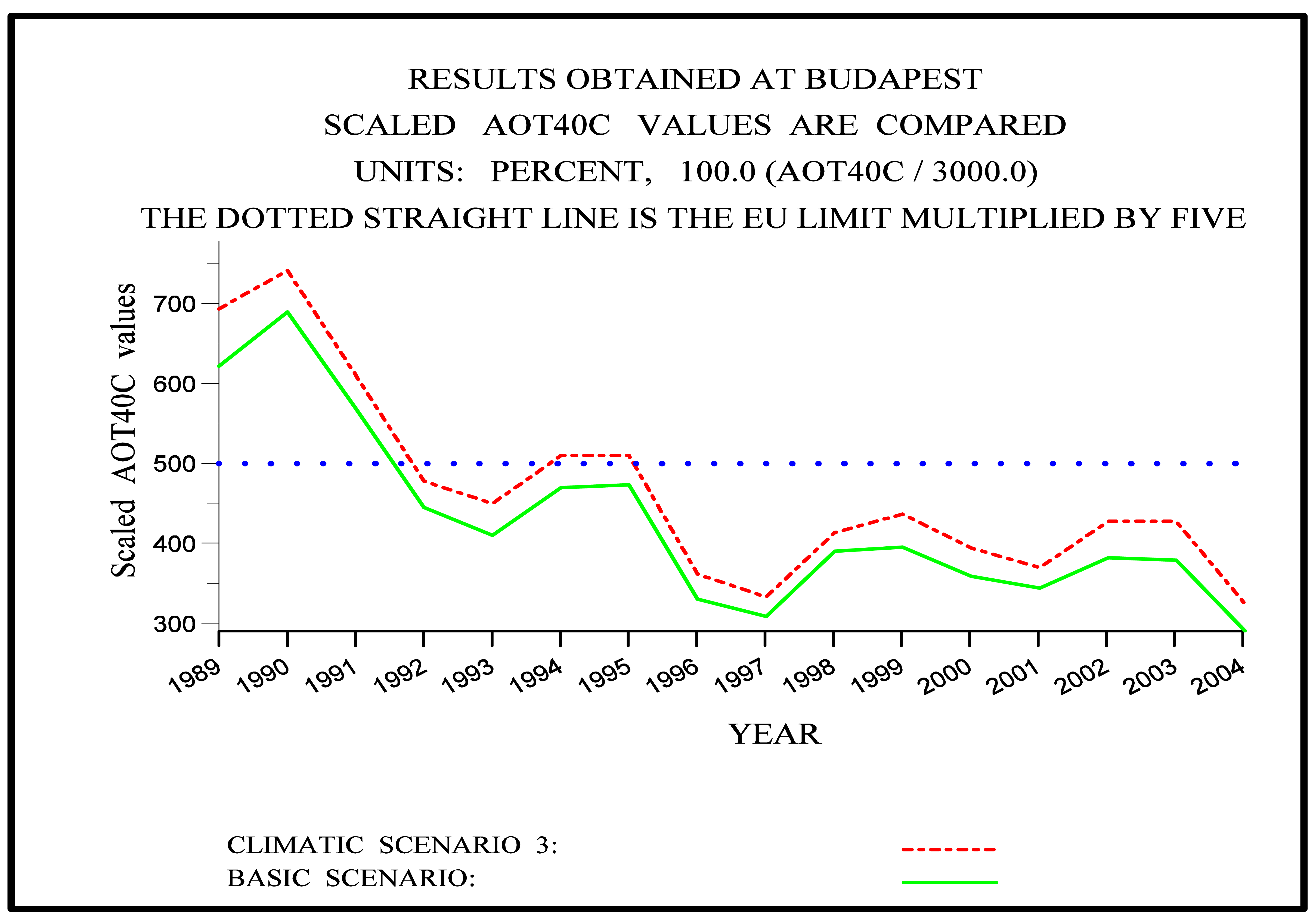
The variation of the AOT40C values near Budapest in the period from 1989 to 2004 is shown in Figure 3. Results related to the AOT40C values for Hungary and its surrounding countries are presented in Figure 4 for year 2004. The results for the other fifteen years can be found on the Internet [33]. More precisely, the quantities in this figure show:
by how much the critical values of AOT40C are exceeded, in percent, both when the Basic Scenario is used (the upper left-hand-side plot) and when IIASA's Maximum Feasible Reduction (MFR) Scenario, see [32], is applied (the lower left-hand-side plot) and
by how much the AOT40C values are changed, in percent, when Climatic Scenario 3 is used instead of the Basic Scenario (the upper right-hand-side plot) and when Climatic Scenario 3 superimposed on the MFR Scenario is used instead of the original MFR Scenario (the upper right-hand-side plot).
The following four conclusions can be drawn by studying the results shown in Figure 3 and Figure 4 (as well as by using some other related results as, for example, those presented in [7]):
The increase of the temperature in Budapest leads to an increase of the AOT40C values for every year of the studied time interval (see Figure 3).
The AOT40C values for 2004, which are obtained by using the Climatic Scenario 3, are greater than the corresponding values obtained by the Basic Scenario in nearly the whole domain containing Hungary and the surrounding countries. In some parts of this domain, the increased values are greater than 30%.
The AOT40C values in Hungary and the surrounding countries exceed several times the EU-limit. The values obtained in the western part of the domain are greater than those in the eastern part. In some areas of the eastern part, the critical level is not exceeded.
If the IIASA MFR Scenario is used, the critical level of 3000 ppb.hours is not exceeded in nearly the whole domain. However, the application of the scenario, in which the climatic changes are taken into account, leads to some increase of the AOT40C values (very often by more than 30%). In this situation this has probably no damaging effects, because the increased values in general remain under the EU critical level.
5. AOT40 Values for Forest Trees
The AOT40 values for forest trees will be denoted as AOT40F and are related to ozone concentrations in the following way (see again [19]):
N is the number of hours in the period from the beginning of April to the end of September, and
ci is the ozone concentration (measured at a given station or calculated by a model at a given grid square) at hour i, where i∈{1, 2,…,N}.
If AOT40F exceeds 10,000 ppb.hours, then this fact may lead to damage of forest trees and, therefore, this situation should be avoided. This critical level is also imposed in [3].
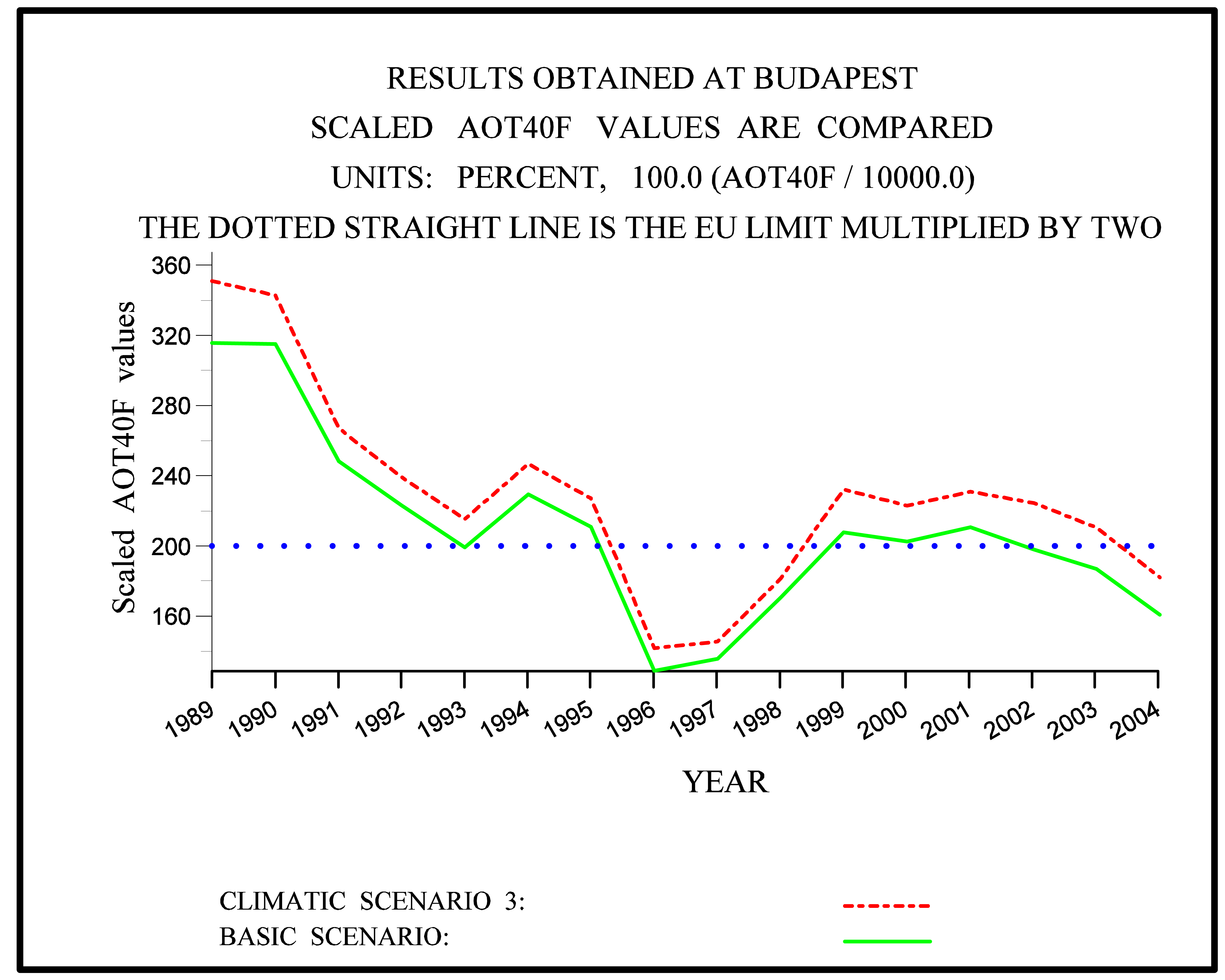
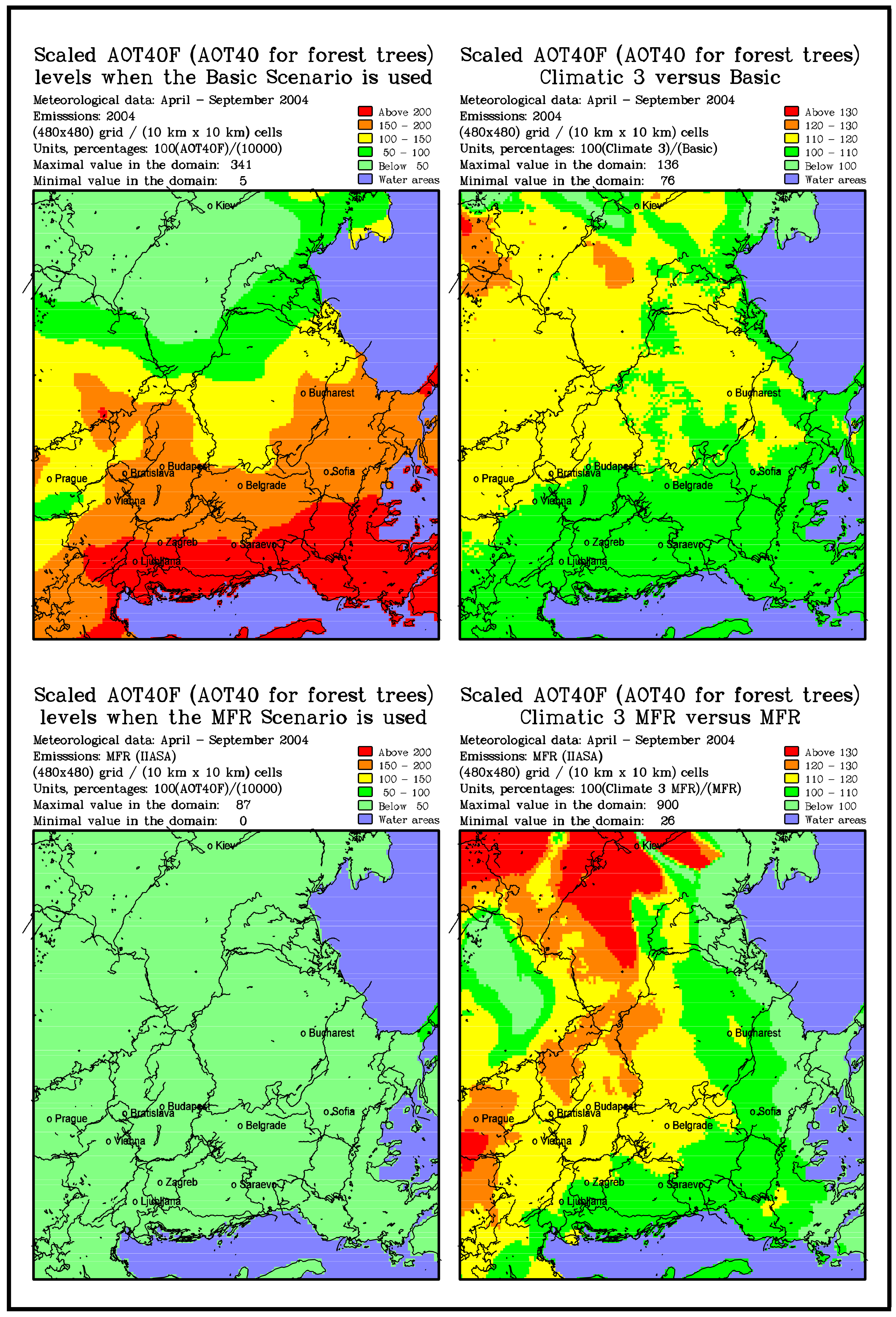
The variation of the AOT40F values near Budapest in the period from 1989 to 2004 is shown in Figure 5. Results related to the AOT40F values for Hungary and its surrounding countries are presented in Figure 6 for year 2004. The results for the other fifteen years can be found on the Internet [34]. More precisely, the quantities in this figure show:
by how much the critical values of AOT40F are exceeded, in percent, both when the Basic Scenario is used (the upper left-hand-side plot) and when IIASA's Maximum Feasible Reduction (MFR) Scenario, see [32], is applied (the lower left-hand-side plot) and
by how much the AOT40F values are changed, in percent, when the Climatic Scenario 3 is used instead of the Basic Scenario (the upper right-hand-side plot) and when the Climatic Scenario 3 superimposed on the MFR Scenario is used instead of the original MFR Scenario (the upper right-hand-side plot).
Several conclusions, which are very similar to those made at the end of Section 4, can be drawn by studying the results in Figure 5 and Figure 6 (as well as by using results from references [5,7,8].
It should be mentioned here that the critical level of 10,000 ppb.hours for AOT40F is not exceeded as much as the critical level of 3,000 ppb.hours for AOT40C (compare the results in Figure 3 and Figure 4 with the corresponding results in Figure 5 and Figure 6).
6. “Bad Days”
Assume that cmax is the maximum of the eight-hour averages of the ozone concentrations calculated by some model or the ozone concentrations measured in a given day at site A. If the condition cmax > 60 ppb is satisfied at least once during the day under consideration, then the expression a “bad day” will be used for such a day at site A. “Bad days” can have damaging effects on some groups of human beings (people who suffer from asthmatic diseases). Therefore, the number of such days should be reduced as much as possible. Two important aims are stated in the Ozone Directive issued by the EU Parliament in year 2002 [3]:
Target aim. The number of “bad days” in any site of the European Union should not exceed 25 after year 2010.
Long-term aim. No “bad day” should occur in the European Union (the year after which the long-term aim has to be satisfied is not specified in the EU Ozone Directive).
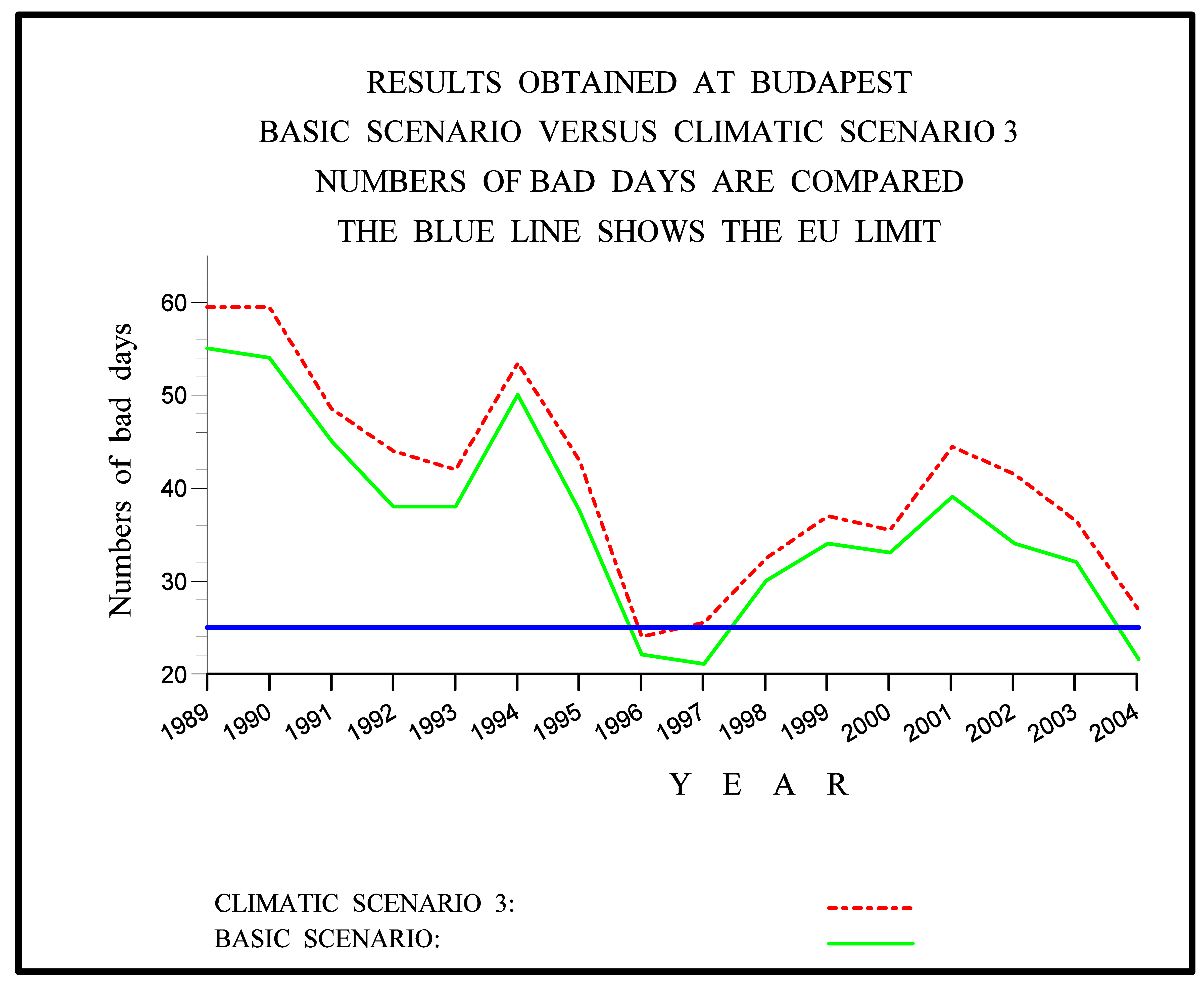
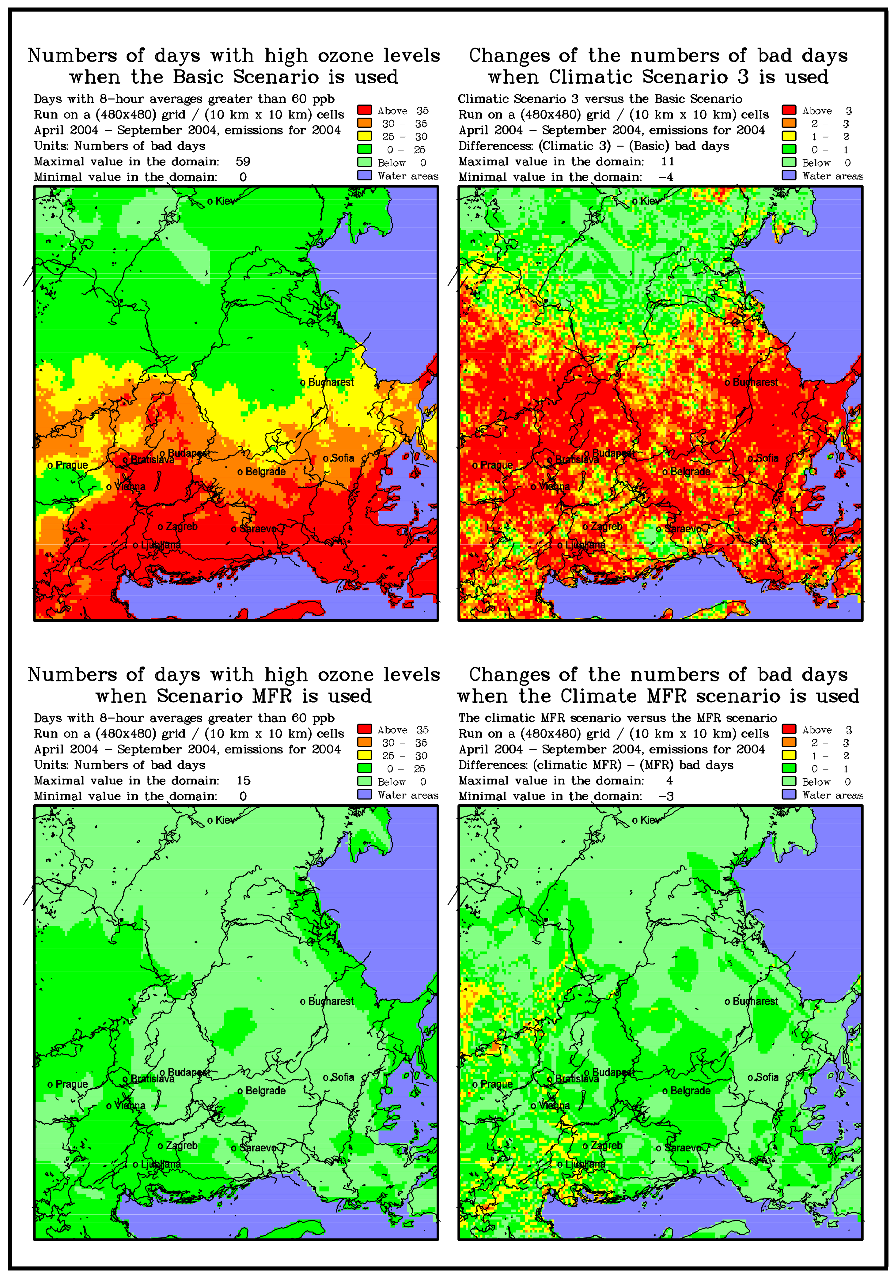
The variation of the numbers of bad days near Budapest in the period from 1989 to 2004 is shown in Figure 7. Results, which are related to distribution of the numbers of bad days in 2004 for Hungary and its surrounding countries, are presented in Figure 8. The results for the other fifteen years can be found on the Internet [34]. The left-hand-side plots in Figure 8 show the numbers of bad days in Hungary and its surrounding countries.
The two right-hand-side plots in Figure 8 show the differences between the bad days obtained by
the Climatic Scenario and the Basic Scenario (the upper plot) and
the Climatic MFR Scenario and the MFR Scenario (the lower plot).
It should be noted that it is not possible to use percentages as in the right-hand-side plots of Figure 4 and Figure 6, because the numbers of bad days are very often reduced to zero when the MFR Scenario is used and it is not possible to form the quantity 100(Climate 3 MFR)/(MFR); thus, it is more appropriate to use the difference (Climate 3 MFR)–MFR).
The increase of the temperature leads to an increase of the numbers of bad days for every year of the studied time interval (see Figure 7).
The numbers of bad days for 2004, which are obtained by using the Climatic Scenario 3, are greater than the corresponding values obtained by the Basic Scenario in a large part of the domain containing Hungary and its surrounding countries. In some parts of this domain the increased values are greater than five days.
The numbers of bad days obtained with the Basic Scenario in the western and southern parts of the studied domain are greater than those in the eastern part. In some areas of the eastern part the critical level is not exceeded (see the upper left-hand-side plot in Figure 8). Also the differences between the numbers of bad days obtained by using the Climatic Scenario 3 and the numbers of bad days obtained by using the Basic Scenario are larger in the western and the southern parts of the studied domain (see the upper right-hand-side plot in Figure 8).
The numbers of bad days are reduced to zero (i.e., the long-term aim in the EU Directive is satisfied) practically in the whole domain when the MFR Scenario is used (see the lower left-hand-side plot in Figure 8). Also the differences between the numbers of bad days obtained by using the Climatic Scenario MFR and the numbers of bad days obtained by using the MFR Scenario are rather small, not greater than four (see the lower right-hand-side plot in Figure 8).
IIASA's MFR Scenario seems to be very efficient in the attempts to reduce the ozone pollution levels (see the results shown in Figure 4, Figure 6 and Figure 8). However, the reductions of the emissions made in the development of this scenario are perhaps too big, see Table 2.
Long-term runs are necessary in the attempts to capture the inter-annual variations. The period of sixteen years chosen in this paper seems to be quite sufficient. The results shown in Table 3 indicate that the inter-annual variations are rather considerable for the chosen period. For example, the maximal numbers of bad days vary from 59 to 83 (see the sixth column in Table 3). However, runs over longer periods (say, 25 or 50 years) might be even more useful.
It is important to ask whether critical levels based on a given number (say, no more than 25 bad days) are relevant. It is not possible to take directly into account the great uncertainties when such critical levels are used. The introduction of uncertainty zones (grey zones), instead of sharp critical levels is proposed and discussed in [8].
4. Concluding Remarks
The influence of the future increases of the temperature on three quantities related to ozone levels in the troposphere is studied in this paper for a spatial domain containing Hungary and its neighboring countries. Special scenarios, which allowed us to compare directly the future and the present levels, were prepared and extensively used. The most important conclusion is that the increases of the temperature do lead to increased pollution levels. It should also be emphasized that measures taken to bring one of the three quantities studied in this paper (AOT40C values, AOT40F values and bad days) under the corresponding critical level does not necessarily mean that the other two quantities will also be under the corresponding critical levels.


| Scenario | Meteorology | Anthropogenic emissions | Biogenic emissions |
|---|---|---|---|
| Basic | EMEP and NERI | EMEP and NERI | Basic |
| Constant Meteorology | Meteorology for 1989 | as in the Basic Scenario | as in the Basic Scenario |
| Constant Emissions | as in the Basic Scenario | Emissions for 1989 | as in the Basic Scenario |
| Climate 3 | Increased temperatures + diurnal and seasonal variations + new humidity and precipitation | as in the Basic Scenario | as in the Basic Scenario |
| MFR Climate MFR | as in the Basic Scenario | Using IIASA factors | as in the Basic Scenario |
| Climate MFR | as in Climate | as in Scenario MFR | as in the Basic Scenario |
MFR: maximum feasible reductions, EMEP: European Monitoring and Evaluation Programme, NERI: National Environmental Research Institute at Aarhus University.
| Country | NOX emissions | VOC emissions |
|---|---|---|
| Hungary | 77% | 75% |
| Romania | 81% | 75% |
| Slovenia | 87% | 78% |
| Croatia | 81% | 76% |
| Austria | 72% | 72% |
| Czech Rep. | 86% | 77% |
| Slovakia | 81% | 62% |
| Ukraine | 83% | 86% |
| Year | AOT40C | AOT40F | Bad days | |||
|---|---|---|---|---|---|---|
| Basic | Climate | Basic | Climate | Basic | Climate | |
| 1989 | 1,445% | 25% | 705% | 20% | 83 | 11 |
| 1990 | 1,455% | 21% | 665% | 15% | 83 | 12 |
| 1991 | 1,307% | 19% | 670% | 16% | 81 | 11 |
| 1992 | 1,410% | 16% | 715% | 16% | 81 | 10 |
| 1993 | 1,400% | 17% | 655% | 17% | 79 | 12 |
| 1994 | 1,315% | 17% | 670% | 17% | 80 | 13 |
| 1995 | 1,553% | 25% | 700% | 20% | 75 | 8 |
| 1996 | 953% | 20% | 460% | 17% | 68 | 10 |
| 1997 | 1,030% | 20% | 565% | 33% | 72 | 10 |
| 1998 | 1,293% | 19% | 570% | 16% | 71 | 10 |
| 1999 | 848% | 95% | 404% | 62% | 70 | 12 |
| 2000 | 872% | 55% | 434% | 37% | 70 | 12 |
| 2001 | 840% | 53% | 372% | 33% | 64 | 12 |
| 2002 | 840% | 36% | 424% | 33% | 68 | 13 |
| 2003 | 812% | 110% | 371% | 53% | 69 | 15 |
| 2004 | 687% | 66% | 341% | 36% | 59 | 11 |
(a) in the second column: MAX(100(AOT40C)/3,000),(b) in the third column: MAX(100(Climate-Basic)/(Basic),(c) in the fourth column MAX(100(AOT40F)/10,000),(d) in the fifth column: MAX(100(Climate-Basic)/(Basic),(e) in the sixth column: maximum of bad days(f) in the seventh column: MAX(Climate-Basic).
Acknowledgments
The work on this project was partly supported by the NATO Scientific Programme (Collaborative Linkage Grants: No. 980505 “Impact of Climate Changes on Pollution Levels in Europe” and No. 98624 “Monte Carlo Sensitivity Studies of Environmental Security”).
The Danish Centre for Supercomputing at the Technical University of Denmark gave us access to several powerful parallel computers for running the long sequence of scenarios.
The European Union and the European Social Fund have provided financial support to the project under the grant agreement no. TÁMOP 4.2.1./B-09/1/KMR-2010-0003.
References
- Athanassiadou, M.; Baker, J.; Carruthers, D.; Collins, W.; Girnary, S.; Hassell, D.; Hort, M.; Johnson, C.; Johnson, K.; Jones, R.; et al. An assessment of the impact of climate change on air quality at two UK sites. Atmos. Environ. 2010, 44, 1877–1886. [Google Scholar]
- Carvalho, A.; Monteiro, A.; Solman, S.; Miranda, A.I.; Borrego, C. Climate-driven changes in air quality over Europe by the end of the 21st century, with special reference to Portugal. Environ. Sci. policy 2010, 13, 445–458. [Google Scholar]
- European Parliament and Council. EC (2002): Directive 2002/3/EC of the European Parliament and the Council of 12 February 2002 relating to ozone in ambient air. OJEC 2002, L67, 14–30. [Google Scholar]
- Zlatev, Z. Computer Treatment of Large Air Pollution Models; Kluwer, Academic Publishers: London, UK, 1995. [Google Scholar]
- Zlatev, Z.; Dimov, I. Computational and Numerical Challenges in Environmental Modeling; Elsevier: Amsterdam, The Netherlands, 2006. [Google Scholar]
- Alexandrov, V.; Owczarz, W.; Thomsen, P.G.; Zlatev, Z. Parallel runs of large air pollution models on a grid of SUN computers. Math. Comput. Simulat. 2004, 65, 557–577. [Google Scholar]
- Csomós, P.; Cuciureanu, R.; Dimitriu, G.; Dimov, I.; Doroshenko, A.; Faragó, I.; Georgiev, K.; Havasi, Á.; Horváth, R.; Margenov, S.; et al. Impact of Climate Changes on Pollution Levels in Europe; NATO: Brussels, Belgium, 2006. Available online: http://www.cs.elte.hu/∼faragois/NATO.pdf (accessed on 10 August 2006).
- Zlatev, Z. Impact of future climate changes on high ozone levels in European suburban areas. Climatic Change 2010, 101, 447–483. [Google Scholar]
- Zlatev, Z.; Moseholm, L. Impact of climate changes on pollution levels in Denmark. Ecol. Model. 2008, 217, 305–319. [Google Scholar]
- Simpson, D.; Guenther, A.; Hewitt, C.N.; Steinbrecher, R. Biogenic emissions in Europe: I. Estimates and uncertainties. J. Geophys. Res. 1995, 100, 22875–22890. [Google Scholar]
- Lübkert, B.; Schöpp, W. The OECD-Map Emission Inventory for, and in Western Europe; Report No. WP-89-082; International Institute for Applied Systems and Analysis (IIASA): Laxenburg, Austria, 1989. [Google Scholar]
- Geernaert, G.; Zlatev, Z. Studying the influence of the biogenic emissions on the AOT40 levels in Europe. IJEP 2004, 23, 29–41. [Google Scholar]
- Anastasi, C.; Hopkinson, L.; Simpson, V.J. Natural hydrocarbon emissions in the United Kingdom. Atmos. Environ. 1991, 25A, 1403–1408. [Google Scholar]
- EMEP (1999): Emission Data: Status Report 1999; EMEP/MSC-W Report 1/99; Meteorological Synthesizing Centre—West, Norwegian Meteorological Institute: Oslo, Norway, 1999.
- EMEP Home Web-page. Avaiable online: http://www.emep.int/index_data.html (accessed on 15 January 2006).
- Hertel, O.; Ambelas Skjøth, C.; Frohn, L.M.; Vignati, E.; Frydendall, J.; de Leeuw, G.; Schwarz, U.; Reis, S. Assessment of the atmospheric nitrogen and sulphur inputs into the North Sea using a Lagrangian model. Phys. Chem. Earth 2002, 27, 1507–1515. [Google Scholar]
- Zlatev, Z.; Syrakov, D. A fine resolution modelling study of pollution levels in Bulgaria. Part 1: SOx and NOx pollution. IJEP 2004, 22, 186–202. [Google Scholar]
- Zlatev, Z.; Syrakov, D. A fine resolution modelling study of pollution levels in Bulgaria. Part 2: High ozone levels. IJEP 2004, 22, 203–222. [Google Scholar]
- Zlatev, Z.; Dimov, I.; Ostromsky, Tz.; Geernaert, G.; Tzvetanov, I.; Bastrup-Birk, A. Calculating losses of crops in Denmark caused by high ozone levels. Environ. Model. Assess. 2001, 6, 35–55. [Google Scholar]
- Abdalmogith, S.; Harrison, R.M.; Zlatev, Z. Intercomparison of inorganic aerosol concentrations in the UK with predictions of the Danish Eulerian Model. J. Atmos. Chem. 2006, 54, 43–66. [Google Scholar]
- Ambelas Skjøth, C.; Bastrup-Birk, A.; Brandt, J.; Zlatev, Z. Studying variations of pollution levels in a given region of Europe during a long time-period. Syst. Anal. Model. Sim. 2000, 37, 297–311. [Google Scholar]
- Bastrup-Birk, A.; Brandt, J.; Uria, I.; Zlatev, Z. Studying cumulative ozone exposures in Europe during a 7-year period. J. Geophys. Res. 1997, 102, 23917–23035. [Google Scholar]
- Dimov, I.; Geernaert, G.; Zlatev, Z. Impact of future climate changes on high pollution levels. IJEP 2008, 32, 200–230. [Google Scholar]
- Zlatev, Z. Massive data sets issues in air pollution modelling. In Handbook on Massive Data Sets in Science and Engineering; Abello, J., Pardalos, P.M., Resende, M.G.C., Eds.; Kluwer Academic Press: London, UK, 2002; pp. 1169–1220. [Google Scholar]
- Havasi, Á.; Bozó, L.; Zlatev, Z. Model simulation on transboundary contribution to the atmospheric sulfur concentration and deposition in Hungary. Idöjárás 2001, 105, 135–144. [Google Scholar]
- Havasi, Á.; Zlatev, Z. Trends of Hungarian air pollution levels on a long time-scale. Atmos. Environ. 2002, 36, 4145–4156. [Google Scholar]
- Harrison, R.M.; Zlatev, Z.; Ottley, C.J. A comparison of the predictions of an Eulerian atmospheric transport chemistry model with experimental measurements over the North Sea. Atmos. Environ. 1994, 28, 497–516. [Google Scholar]
- Hass, H.; van Loon, M.; Kessler, C.; Stern, R.; Mathijsen, J.; Sauter, F.; Zlatev, Z.; Langner, J.; Foltescu, V.; Schaap, M. Aerosol Modelling: Results and Intercomparison from European Regional-Scale Modelling Systems; GSF—National Research Center for Environment and Health, International Scientific Secretariat (ISS), EUROTRAC-2: Münich, Germany, 2004. Available online: http://www.trumf.fu-berlin.de/veranstaltungen/events/glream/GLOREAM_PMmodel-comparison.pdf (accessed on 15 December 2004).
- Roemer, M.; Beekman, M.; Bergsröm, R.; Boersen, G.; Feldmann, H.; Flatøy, F.; Honore, C.; Langner, J.; Jonson, J.E.; Matthijsen, J.; et al. Ozone Trends According to Ten Dispersion Models; GSF—National Research Center for Environment and Health, International Scientific Secretariat (ISS), EUROTRAC-2: Munich, Germany, 2004. Available online: http://www.mep.tno.nl/eurotrac/EUROTRAC-trends.pdf (accessed on 15 December 2004).
- Houghton, J.T.; Ding, Y.; Griggs, D.J.; Noguer, M.; van der Linden, P.J.; Dai, X.; Maskell, K.; Johnson, C.A. Climate Change 2001: The Scientific Basis; Cambridge University Press: Cambridge, UK, 2001. [Google Scholar]
- In Climate Change (2007): The Physical Science Basis; Contribution of the Working Group I to the Fourth Assessment Report of IPCC (Intergovernmental Panel on Climate Change). Cambridge University Press: Cambridge, UK, 2007.
- Amann, M.; Bertok, I.; Cofala, J.; Gyarfas, F.; Heyes, C.; Klimont, Z.; Makowski, M.; Schöpp, W.; Syri, S. Cost-Effective Control of Acidification and Ground-Level Ozone; Seventh Interim Report; International Institute for Applied System Analysis (IIASA): Laxenburg, Austria, 1999. [Google Scholar]
- Interim Reports to the European Commission for the Directive on National Emission Ceilings and the EU Ozone Strategy; International Institute for Applied Systems Analysis (IIASA): Laxenburg, Austria, 2000. Available online: http://www.iiasa.ac.at/∼rains/interim_reports.html (accessed on 23 May 2000).
- Zlatev, Z.; Havasi, Á.; Faragó, I. Influence of Climatic Changes on Pollution Levels in Hungary and Its Surrounding Countries (Extended Version); Matematikai Intézet: Budapest, Hungary, 2011. Available online: http://www.cs.elte.hu/∼faragois/climatic_scenarios_hungary_extended_version.doc (accessed on March 30 2011).
© 2011 by the authors; licensee MDPI, Basel, Switzerland. This article is an open access article distributed under the terms and conditions of the Creative Commons Attribution license (http://creativecommons.org/licenses/by/3.0/).
Share and Cite
Zlatev, Z.; Havasi, Á.; Faragó, I. Influence of Climatic Changes on Pollution Levels in Hungary and Surrounding Countries. Atmosphere 2011, 2, 201-221. https://doi.org/10.3390/atmos2030201
Zlatev Z, Havasi Á, Faragó I. Influence of Climatic Changes on Pollution Levels in Hungary and Surrounding Countries. Atmosphere. 2011; 2(3):201-221. https://doi.org/10.3390/atmos2030201
Chicago/Turabian StyleZlatev, Zahari, Ágnes Havasi, and István Faragó. 2011. "Influence of Climatic Changes on Pollution Levels in Hungary and Surrounding Countries" Atmosphere 2, no. 3: 201-221. https://doi.org/10.3390/atmos2030201