Surface Flux Modeling for Air Quality Applications

Abstract

For many gasses and aerosols, dry deposition is an important sink of atmospheric mass. Dry deposition fluxes are also important sources of pollutants to terrestrial and aquatic ecosystems. The surface fluxes of some gases, such as ammonia, mercury, and certain volatile organic compounds, can be upward into the air as well as downward to the surface and therefore should be modeled as bi-directional fluxes. Model parameterizations of dry deposition in air quality models have been represented by simple electrical resistance analogs for almost 30 years. Uncertainties in surface flux modeling in global to mesoscale models are being slowly reduced as more field measurements provide constraints on parameterizations. However, at the same time, more chemical species are being added to surface flux models as air quality models are expanded to include more complex chemistry and are being applied to a wider array of environmental issues. Since surface flux measurements of many of these chemicals are still lacking, resistances are usually parameterized using simple scaling by water or lipid solubility and reactivity. Advances in recent years have included bi-directional flux algorithms that require a shift from pre-computation of deposition velocities to fully integrated surface flux calculations within air quality models. Improved modeling of the stomatal component of chemical surface fluxes has resulted from improved evapotranspiration modeling in land surface models and closer integration between meteorology and air quality models. Satellite-derived land use characterization and vegetation products and indices are improving model representation of spatial and temporal variations in surface flux processes. This review describes the current state of chemical dry deposition modeling, recent progress in bi-directional flux modeling, synergistic model development research with field measurements, and coupling with meteorological land surface models.

1. Introduction

Atmospheric modeling systems that simulate meteorology, chemistry, or climate include model algorithms for air-surface exchange processes. Surface fluxes of heat, moisture, and momentum are critical elements of meteorology and climate models while chemistry/air quality models also require algorithms for surface fluxes of trace chemical species. Vertical flux of any quantity in the atmospheric surface layer is well described by gradient turbulent diffusion. Momentum flux can be modeled simply by means of turbulent surface layer similarity theory since momentum goes to zero at some finite height, known as the roughness length (z_o), which depends on the characteristics of the surface and vegetation. Sensible heat flux is slightly more complex than momentum flux since thermal exchange processes must interact directly with the surface and turbulent flow cannot extent all the way to the surface because of the “no-slip” condition. Thus, for heat there is an additional consideration of laminar molecular diffusion over a very thin layer in contact with all ground and canopy surfaces. Modeling moisture fluxes adds another element of complexity because of the multiple sources of surface moisture, via evapotranspiration (ET), which is regulated by leaf stomata, soil moisture, which requires diffusion through soil, and surface wetness from rain and dew. The surface fluxes of many chemical species that are involved in air quality modeling have similarities to moisture fluxes, since they may also involve multiple pathways for exchange with the surface, including stomatal, ground, water, built surfaces, and leaf cuticles. For example, in two different field experiments where both moisture fluxes and ozone fluxes were measured by eddy covariance, one for a vineyard and cotton field in California [1] and another for a soybean field in Kentucky [2], the stomatal pathway for ozone and water vapor fluxes were shown to be highly correlated. Thus, modeling chemical dry deposition and bi-directional surface fluxes involve many of the same physical processes and can use many common algorithms with moisture flux calculations in the land surface models of meteorology and climate models, especially for the stomatal component.

While chemical constituents of the atmosphere can undergo a variety of chemical and physical transformations, dry and wet deposition are the ultimate removal mechanisms of mass emitted to the atmosphere. Surface fluxes of some chemical species, notably ammonia [3–5], mercury [6,7], and certain volatile organic compounds (VOCs) [8] are often bi-directional, such that the surface may be alternately a source or sink of atmospheric mass. For other chemicals, particularly biogenic VOCs such as isoprene, terpenes, and alcohols the surface emissions from biological processes are very important atmospheric sources [9].

In addition to their roles as sources and sinks of atmospheric constituents, surface fluxes also have important effects on vegetation, ecosystems, and human health. Risk assessments and setting standards for protecting vegetation and ecosystems from damage by air pollutants has usually involved concentration based indexes such as AOT40 (Accumulated Over a Threshold of 40 ppb) which is used for assessing ozone impacts. A new flux based index called AFstY (Accumulated stomatal Flux above a flux threshold Y) has been proposed to estimate O₃ dose to leaf interiors where damage occurs rather than in the air outside the leaf [10]. A recent study in Europe used the Deposition of Ozone and Stomatal Exchange (DO3SE) model to compute the AFstY index to assess the O₃ impacts on key European tree species [11,12]. Their results showed that the AFstY index differed significantly from the AOT40 over different regions and species.

Until recently, secondary standards for protecting ecosystems from damage caused by NOx and SOx in the U.S. have been based on ambient concentrations even though flux based standards were proposed more than 10 years ago [13]. Recently, however, new SOx-NOx secondary standards are being considered to protect both terrestrial and aquatic ecosystems from acidification and nutrient enrichment. Although the U.S. Clean Air Act requires that regulations must be based on ambient concentration levels, the newly proposed standards include linkages to deposition of SOx and NOx [14] to be computed by the Community Multiscale Air Quality CMAQ model [15]. Therefore, chemical surface flux modeling has become a more important process in air quality models used for regulation assessment and enforcement because environmental standards are now being promulgated that include assessments of deposition effects on ecosystems.

Since industrialization, atmospheric reactive nitrogen concentrations and deposition have increased tremendously [16–18]. Deposition of reactive nitrogen including, ammonia, NO₂, nitric acid, ammonium and nitrate containing aerosols, and organic nitrates has serious deleterious impacts on terrestrial and aquatic ecosystems [19–21]. Thus, modeling anthropogenic and natural emissions, chemical transformations, wet deposition, and surface fluxes is important not only for air quality studies but also for ecosystem impact assessments. Ammonia from fertilizer and livestock operations contribute the largest portion of excess nitrogen emissions to the environment [22]. Accurate accounting of fertilizer sources of ammonia requires development of new modeling techniques such as bi-directional surface fluxes, as well as integration with agricultural management models (see Section 3.3).

This article presents an overview of the current state of science and modeling for surface flux processes in air quality modeling systems. We start with a presentation of the governing principles and equations of air-surface exchange that are applicable to moisture, heat, and momentum in meteorology models and chemical surface fluxes in chemical transport models in Section 2. Then, in Section 3 we focus on modeling techniques for chemical surface fluxes, including gas and aerosol dry deposition and bi-directional fluxes. Section 4 gives an overview of recent advances in dry deposition and bi-directional modeling along with a few examples of model results. Section 5 contains a concluding discussion of limitations of current models and future research and model development directions. As developers of land surface models (LSM) [23,24], dry deposition [25], and bidirectional models [26] we often use the formulation of these models as they are applied in the Weather Research and Forecast (WRF) model [27] and the CMAQ model as examples of parameterization techniques and to illustrate some of the characteristics of model results. Note that much of the description of the dry deposition model used in CMAQ has not been previously published.

2. Governing Principles of Surface Fluxes Modeling

Turbulent fluxes of any atmospheric quantity, including heat, moisture, momentum and trace chemical species, can be computed according to Monin-Obukov similarity theory in the atmospheric surface-layer which relates fluxes at height z near the surface to the mean vertical profile:

$$F_{\mathit{\alpha }}(z)=\overline{w\prime \mathit{\alpha }\prime }=\frac{u_{*}kz}{{\mathit{\varphi }}_h\left(\frac{z}{L}\right)}\frac{\partial \mathit{\alpha }}{\partial z}$$

(1)

where F_α is the vertical flux of any quantity α, which can be measured as the mean value of the turbulent covariance of w and α wherever stationarity and horizontal homogeneity can be reasonably assumed. Also, u* is the surface friction velocity, k is the von Karman constant, ϕ_m and ϕ_h are non-dimensional profile functions derived empirically from observed data, and L is the Monin-Obukov length scale which is defined as:

$$L=\frac{T_o{u}_{*}^3}{gk<w\prime T_o\prime >})$$

(2)

where <w′T_o′> represents the kinematic heat flux and T_o represents the average temperature in the surface layer. Assuming constant flux between some reference height z_r within the surface layer and the surface, Equation 1 can be vertically integrated to give:

$$F_{\mathit{\alpha }}=\frac{u_{*}k(\mathit{\alpha }(z_r)-{\mathit{\alpha }}_o)}{{\varphi }_{hn}\left[\mathit{ln}\left(\frac{z}{z_o}\right)-{\mathit{\psi }}_h\left(\frac{z}{L},\frac{z_o}{L}\right)\right]}$$

(3)

where ϕ_hn is the non-dimensional temperature profile constant for neutral conditions, ψ_h is the stability correction function for heat, and α_o is the value of α at a micro-distance above the surface where turbulence cannot penetrate. Equation (3) can be rewritten as:

$$F_{\mathit{\alpha }}=\frac{(\mathit{\alpha }(z_r)-{\mathit{\alpha }}_o)}{R_a},R_a=\frac{{\mathit{\varphi }}_{hn}}{u_{*}k}\left[\mathit{ln}\left(\frac{z}{z_o}\right)-{\mathit{\psi }}_h\left(\frac{z}{L},\frac{z_o}{L}\right)\right]$$

(4)

where R_a is generally known as the aerodynamic resistance. However, Equation (4) by itself is not very useful because of the difficulty in measuring or modeling quantities at a tiny distance above the surface. We would rather replace α_o with α_s (the quantity at the surface) which can be measured, estimated from surface properties, or assumed to equal zero, as for dry deposition. Again assuming that the flux is constant down to the surface, we can define two more resistances for the quasi-laminar boundary layer (R_b), which is the non-turbulent micro layer adjacent to all surfaces, and a surface resistance (R_s):

$$F_{\mathit{\alpha }}=\frac{({\mathit{\alpha }}_o-{\mathit{\alpha }}_{\mathit{\delta }})}{R_b}=\frac{({\mathit{\alpha }}_{\mathit{\delta }}-{\mathit{\alpha }}_s)}{R_s}$$

(5)

where α_δ represents the quantity α in the air at the surface. Combining Equations (4) and (5) yields:

$$F_{\mathit{\alpha }}=\frac{(\mathit{\alpha }(z_r)-{\mathit{\alpha }}_s)}{R_a+R_b+R_s}$$

(6)

For dry deposition α _s is assumed to be zero and Equation 6 is expressed as:

$$F_{\mathit{\alpha }}=V_d\mathit{\alpha }(z_r),V_d=\frac{1}{R_a+R_b+R_s}$$

(7)

For bi-directional surface flux Eq 6 can be more complicated because α_s may be different for various components of the surface such as the ground and vegetation canopy as described in section 3.3.

R_a represents the resistance to flux by turbulent diffusion through the turbulent surface layer while R_b represents molecular or Brownian diffusion across a very thin quasi-laminar boundary layer adjacent to the surface. A general form of R_b for any scalar quantity was recommended by Wesely and Hicks [28] as:

$$R_b=\frac{B^{-1}}{u_{*}}{\left(\frac{Sc}{Pr}\right)}^{\stackrel{2}{}/\underset{3}{}}$$

(8)

where Sc is the Schmidt number (Sc = v/D), with ν representing the kinematic molecular viscosity, and D is the molecular diffusivity of the scalar quantity. Pr is the Prandtl number, which is the analogous quantity for heat (Pr = v/v_θ), where v_θ is the molecular thermal diffusivity. The parameter B⁻¹ is the inverse Stanton number, a dimensionless heat transfer coefficient. The value of B⁻¹ may depend on the Reynolds number as well as the type of surface roughness. For example, Garratt and Hicks [29] suggested a value of kB⁻¹ = 2 for fully turbulent flow over fibrous vegetative canopies.

Note that, since R_a represents the aerodynamic properties of the turbulent surface layer which depends purely on meteorological parameters and surface characteristics (i.e., surface roughness) it is independent of the chemical or physical properties of the transported scalar. Thus, R_a,once computed, can be used in the surface flux calculations of any scalar. R_b, however, combines meteorological and fluid flow parameters (i.e., u_* and B) with properties of the transported scalar (i.e., molecular diffusivity) and must be computed individually for each chemical species.

3. Chemical Surface Fluxes

Chemical surface fluxes are partially analogous to moisture fluxes, especially for the stomatal conductance, which can be adapted to any gas by scaling by the ratio of molecular diffusivity of the chemical species to the molecular diffusivity of water vapor.

3.1. Dry Deposition Modeling

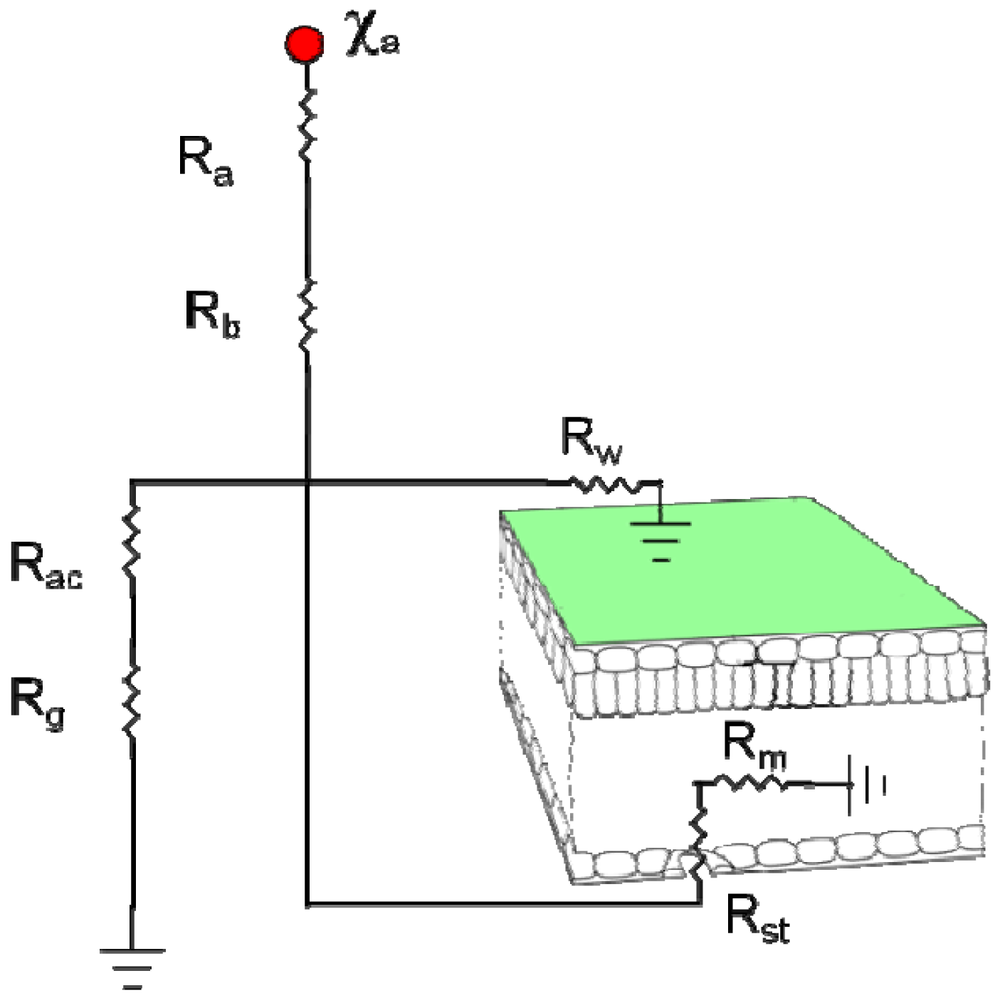
For chemical species which are dominated by one-way flux to the surface, the surface concentration is assumed to be zero. Thus, for such chemical scalars the gradient flux across the air-surface interface is always directed toward the surface no matter how low the air concentration. This special case is simplified as shown by Equation 7, where the flux is a simple linear combination of air concentration near the surface and the deposition velocity V_d. The surface resistance R_s represents all pathways for sinks of atmospheric chemical species to the surface. The major pathways for trace gasses include stomatal uptake, deposition to leaf cuticles, and deposition to ground surfaces. The relative importance of these pathways for any particular chemical species depends on their chemical and physical properties, such as solubility, reactivity, and molecular diffusivity. For example, nitric acid is both highly soluble and highly reactive such that its surface resistance is effectively zero (compared to R_a and R_b) [30,31]. Therefore, the deposition velocity of nitric acid can be estimated reasonably well as: 1/(R_a + R_b). For other less reactive gasses the surface resistance is more important and each of the main pathways may contribute significantly to the surface flux. The simplest representation of R_s for a single layer or “Big Leaf” model is represented as a combination of parallel resistances given by:

$$R_s={\left(\frac{1}{R_{\mathit{\text{st}}}}+\frac{1}{R_w}+\frac{1}{R_g}\right)}^{-1}$$

(9)

where R_st is stomatal resistance, R_w is cuticular resistance, and R_g is ground resistance.

However, since leaves are displaced above the ground there should be additional resistance for the ground pathway to account for transport through the plant canopy. Furthermore, some models account for concentration gradients within the canopy by using a multilayer approach to account for the vertical distribution of leaf surface area [32,33]. Multilayer models can also calculate the light attenuation within the canopy and thereby more accurately represent the fraction of sunlit and shaded leaves at each level which has significant influence on stomatal resistance (see below the section on Scaling from Leaf to Canopy). For large scale air quality modeling, however, the complication of multi-layer models is usually not desired since the variety of vegetation contained within the large areas represented by each model grid cell is not amenable to realistic representation of canopy structure. Alternatively, a simple in-canopy resistance can be added in series with the ground surface resistance. For example, Erisman et al. [34] suggested:

$$R_{ac}=b\frac{h_{c}LAI}{u_{*}}$$

(10)

where LAI is the one-sided leaf area index, h_c the canopy height and b an empirical constant taken as 14 m⁻¹. Zhang et al. [35] developed a similar parameterization for R_ac related to LAI and u_* that includes variations by land use category and day of the year to account for changes in canopy structure.

Another complication is that there may be an additional resistance to absorption into the mesophyll tissue inside the stomatal cavity of the leaf for some chemicals. Thus, including a mesophyll resistance R_m and R_ac, the total R_s becomes:

$$R_s={\left(\frac{1}{R_{\mathit{\text{st}}}+R_m}+\frac{1}{R_w}+\frac{1}{R_{ac}+R_g}\right)}^{-1}$$

(11)

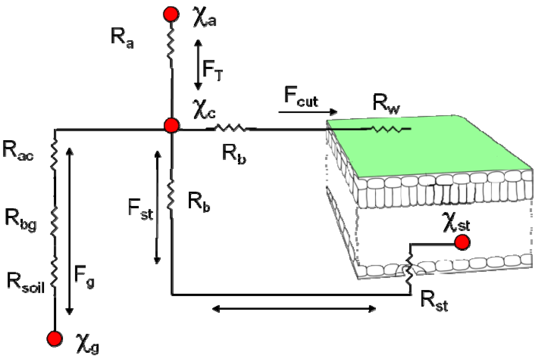
Thus, dry deposition velocity V_d can be represented by resistances in series and parallel as shown in Figure 1.

3.1.1. Stomatal Resistance

All gasses diffuse through stomata when they are open. The stomatal pathway is particularly important for some chemical species such as O₃, NH₃, CO₂, NO₂, and SO₂. While O₃ and SO₂ deposit readily via the stomatal pathway with little or no mesophyll resistance, stomatal uptake of other less soluble gasses, such as NO, NO₂, and CO, is limited by various magnitudes of mesophyll resistance. Several biologically active chemicals such as CO₂ and NH₃ can flux through the stomata in both directions depending on the concentration gradient between the stomatal cavity and the external air. Techniques for modeling bidirectional flux are discussed in Section 3.3.

Stomatal resistance or conductance (g_st = 1/R_st) controls the flux of gasses, including CO₂ and water vapor, into and out of leaves. Since stomatal resistance is the primary regulatory process for evapotranspiration, it is a key parameter for LSMs that are included in meteorology models. Thus it makes sense to use the same parameterization of the stomatal pathway for the meteorological and chemical components of air quality modeling systems [25].

The primary function of leaf stomata is to allow the intake of CO₂ for photosynthesis while minimizing the cost of water vapor loss to the atmosphere. In addition, the diffusion of water out of stomata into the atmosphere (leaf transpiration) is the major mechanism for mass flow of liquid water with any dissolved mineral nutrients from the roots to the leaves through the xylem. Stomatal opening responds to environmental conditions, including sunlight, humidity, temperature, soil moisture, CO₂ concentration, and nutrient availability. Stomatal conductance, which is directly related to the degree of stomatal opening, is usually modeled in LSM and dry deposition models following either the empirical approach of Jarvis [36] or photosynthesis-based semi-empirical models [37–40].

The Jarvis model uses a series of empirical functions as linear coefficients to the maximum stomatal conductance g_smax (conductance at maximum opening), which is a characteristic of each plant reflecting the size and density of stomata. For example, Pleim and Xiu [41] used this approach in their LSM that is in the WRF model and for dry deposition in the CMAQ model to model bulk (canopy level) stomatal conductance g_sb as:

$$g_{sb}=\frac{g_{\mathit{\text{smax}}}{F}_1(\mathit{\text{PAR}})F_2(w_2)F_3(R{H}_s)F_4(T_a)}{\mathit{\text{LAI}}}$$

(12)

where the functions F_1–4 represent the fractional degree of stomatal closure caused by the environmental stresses: photosynthetically active radiation PAR, root-depth soil moisture w₂, relative humidity at the leaf surface RH_s, and air temperature in the canopy T_a. Note that the scaling up from leaf to canopy appears from Equation (12) to be simply a linear dependence on LAI. There is, however, an additional dependence on LAI in the F₁ term that accounts for increased shading in denser canopies [42]. Discussion of simple and more detailed techniques for scaling from leaf to canopy is presented below. The Jarvis-type empirical stomatal conductance model has been widely used in LSM components of meteorology [23,43,44] and dry deposition models [32,45,46].

The photosynthesis approach solves for stomatal conductance assuming that CO₂ diffusion through the stomata is equal to the net CO₂ assimilation rate for photosynthesis minus respiration. These models originated in plant biochemical studies [38,39] and are widely used in ecology and hydrology models and were later adapted for use in atmospheric models [40,47]. Based on the optimality hypothesis of the study by Cowan [37] plants optimize their stomatal conductance for maximizing photosynthesis at a given amount of transpiration. Photosynthesis-based models are used in the third and fourth generations of LSMs in Global Climate Models (GCM) for modeling ET and the carbon cycle [48–51]. The semi-empirical Ball-Berry model [39] computes stomatal conductance based on:

$$gs=\frac{a_{1}A{F}_h}{c_s}+g_o$$

(13)

where F_h is an empirical function of humidity, A is the CO₂ assimilation rate, c_s is the CO₂ concentration at the leaf surface, a₁ is an empirical coefficient, and g_o is the minimum stomatal conductance. These models have the advantage of describing the rate of photosynthesis in a mechanistic fashion thereby providing a theoretical basis for stomatal response to environmental conditions such as temperature, solar radiation, water stress, and nutrient availability. However, there is no theoretical basis for response to air humidity or soil moisture. Since these models are combinations of theoretical biochemistry and empirical parameterizations, their predicted stomatal response to each independent environmental variable is not clearly evident. Thus the photosynthesis approach is semi-empirical, since the parameters a₁ and g_o are empirically estimated for each plant type. Also, F_h is an empirical function of air humidity that is similar to F₃ in Equation (12). While Jarvis-type models typically use simple functions of ambient vapor pressure deficit (D_a = e_sat − e_a) [43] the photosynthesis based models alternatively use F_h = RH_s [39] or F_h = (1 + D_s/D_o)⁻¹ as suggested by Lohammer et al. [52], where D_s is the vapor pressure deficit at the leaf surface (D_s = e_sat − e_s) and D_o is an empirical constant. Note that the Lohammer humidity function results from a linear relationship between g_s and ET, which has often been observed in laboratory experiments [40,53]. While F_h in Equation (13) and F₃ in Equation (12) seem to be equivalent, Aphalo and Jarvis [54] pointed out that since the assimilation rate has an implicit dependence on humidity, F_h does not encapsulate the entire humidity dependence of these models. Pleim [55] analyzed the three humidity functions and found that for use in a Jarvis-type model F₃ = RH_s is most appropriate and, therefore, is now used in the Pleim-Xiu LSM [24].

Recently, many LSM formulations in climate models [48,56,50] have used the photosynthesis approach to stomatal conductance. Such models have a distinct advantage over models using the Jarvis empirical approach because of the explicit dependence of stomatal conductance on CO₂ concentration. Thus, feedbacks of increasing CO₂ on ET can be included in future GCM projection simulations. While biochemical stomatal models have been developed and tested for LSM and dry deposition for use in meteorology and air quality models [33,57–59] they have yet to be applied in operational mesoscale models.

3.1.2. Cuticle Resistance

Leaf cuticles are impregnated with waxy substances that resist water loss. Thus, evaporative fluxes from leaf surfaces (non-stomatal) occur only from external wetness from rain or dew. For some trace chemicals, however, deposition to dry leaf cuticles is a significant process for removal. Chemical deposition to wet leaves scales with Henry's law of solubility with a dependence on pH for species that readily dissociate in the aqueous phase (e.g., SO₂ and NH₃) [60,61]. Mechanisms for deposition to dry cuticles are less well understood. Some dry deposition models simply specify constant values for cuticle resistance or even total canopy resistance for each chemical species based on empirical fits to observations without attempting to hypothesize about the mechanism [62–64]. The problem with this approach is that it is limited to the few gasses for which field flux measurements have been made in a variety of landscapes. Other models generalize the calculation of cuticular resistance based on chemical properties such as a reactivity factor [35,60,61,65] so that estimates for R_w can be made even for species for which surface fluxes have not been measured in the field. Some models also include a dependence of R_w on Henry's law coefficient and/or RH even for dry cuticles particularly for highly soluble chemicals like NH₃ and SO₂ [34]. Jones et al. [66] found that the R_w for ammonia is a linear function of NH₃ concentration, suggesting an inhibiting effect caused by saturating the cuticular membrane. For hydrophobic organic chemical species it has been hypothesized that a small amount of mass may dissolve into the wax-like lipids in the leaf cuticle and then diffuse through the cuticle to the leaf interior. Thus, R_w for chemicals that have low water solubility but high lipid solubility may be parameterized using the octanol-water partitioning coefficient [33,67]. The R_w values computed by such parameterizations are usually quite high resulting in very small fluxes. However, for toxic organic chemicals, often known as persistent organic pollutants (POPs), absorption into leaf cuticle of even small quantities is an important pathway for contamination of vegetation that can subsequently enter the food chain [68].

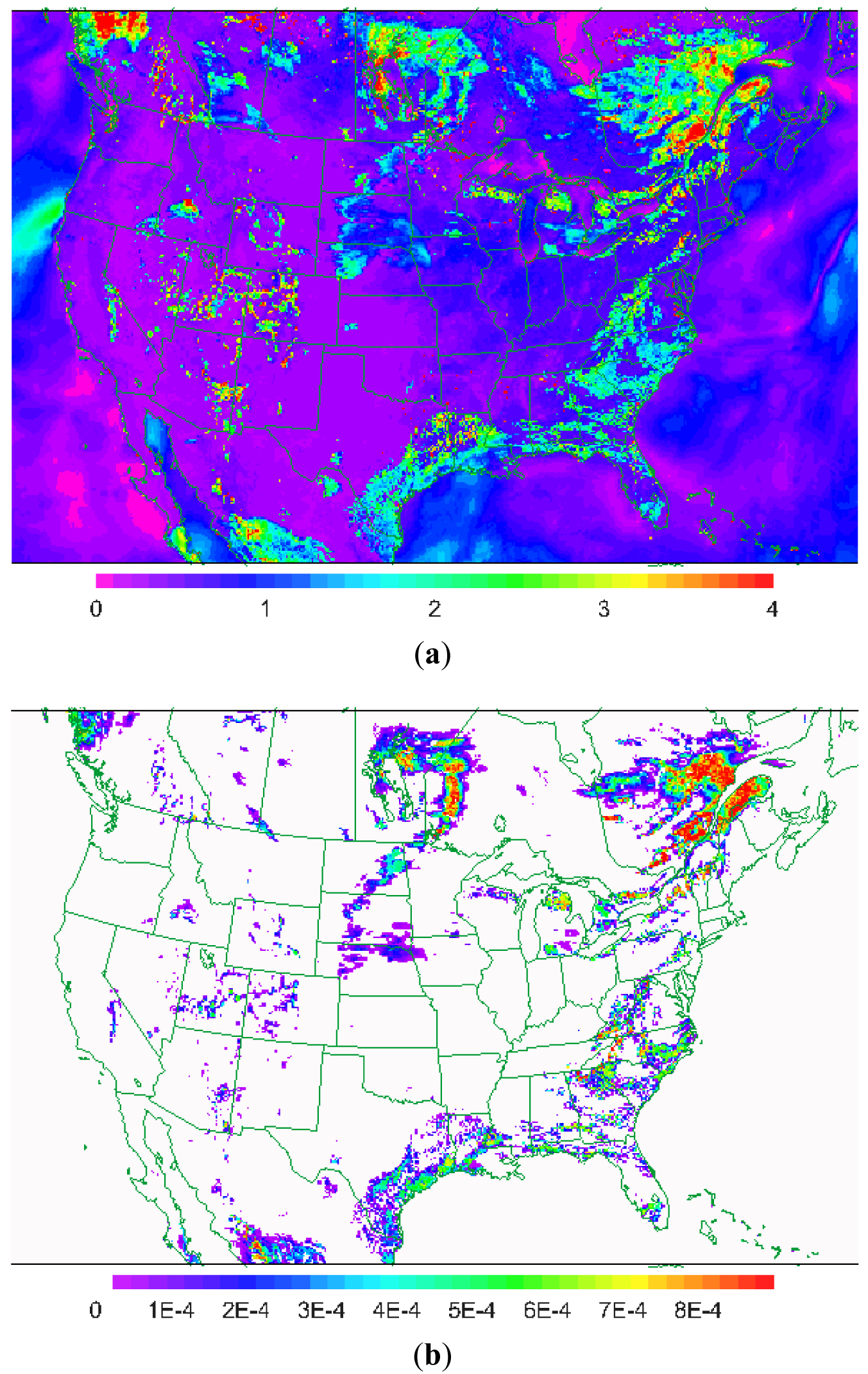
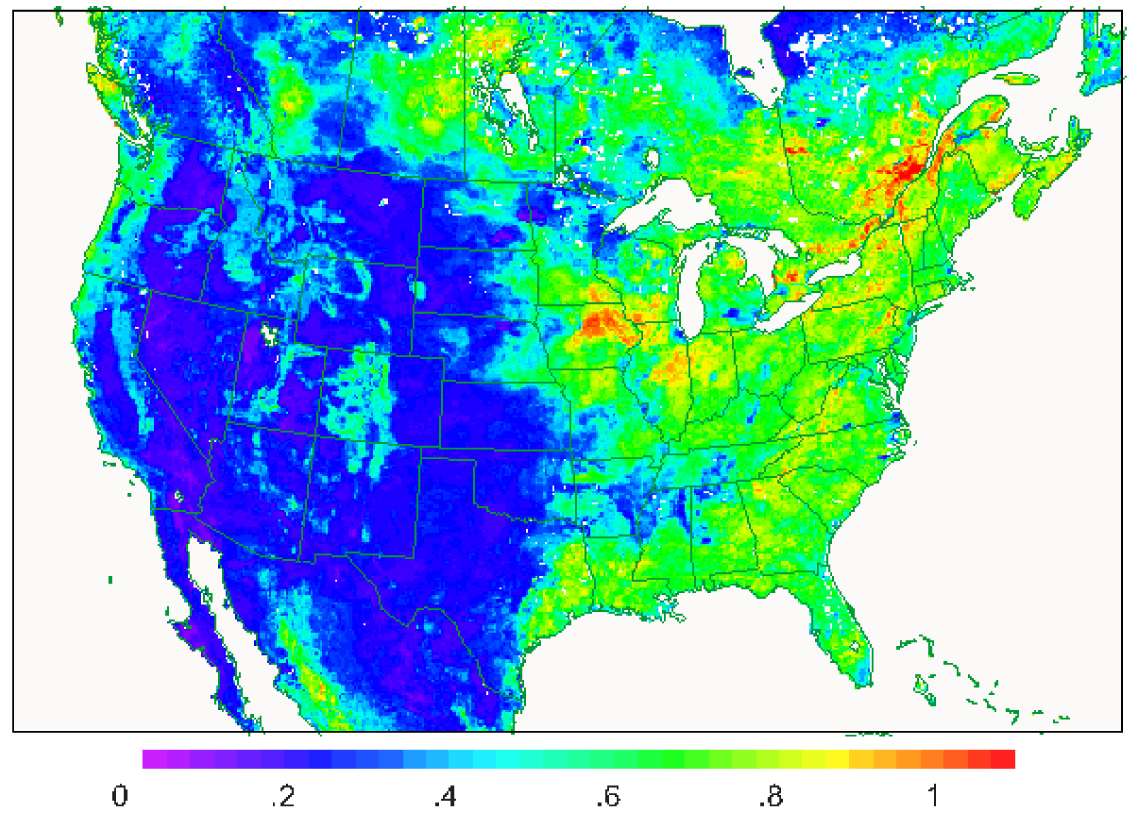
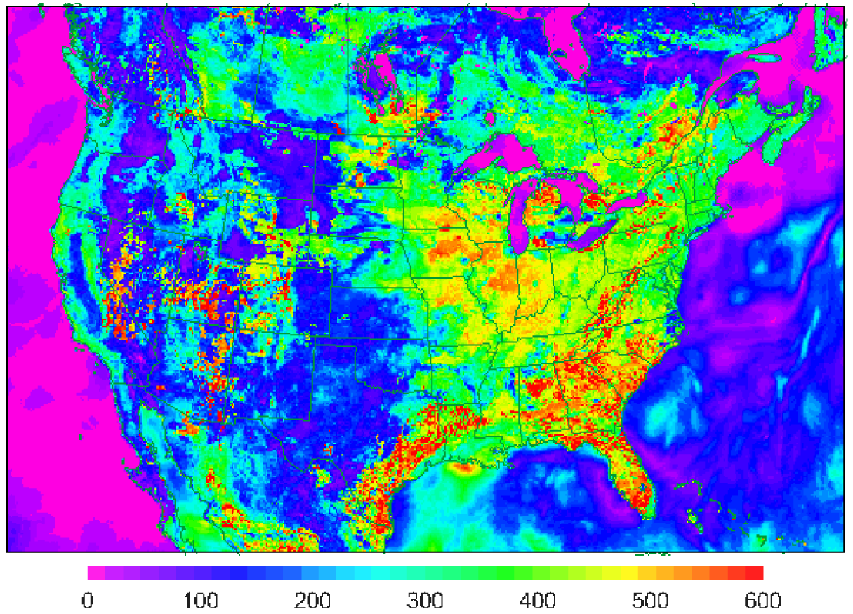
The dominant mechanism for cuticular deposition depends on the properties of chemical species. Soluble species such as SO₂, H₂O₂, and NH₃ quickly dissolve into water on leaves that are wetted by rain or dew. Cuticle resistance is very low for these species when leaves are wet but resistance for dry portions of the leaves can be quite high leading to low deposition velocities in dry areas. For example, Figure 2a shows the dry deposition velocity for SO₂ from the WRF-CMAQ model system in mid-afternoon (20 UT) on July 25, 2006 on a 12 km model grid. Note that the distinct pattern of high deposition velocities closely follows the pattern of canopy water content shown in Figure 2b. Thus, it is important to account for parallel pathways to wet and dry portions of the leaves and couple the dry deposition calculation to a realistic treatment of canopy water. For the example shown in Figure 2 the dry deposition model in CMAQ is coupled to the PX LSM in WRF which integrates canopy water as a prognostic variable.

3.1.3. Ground Resistance

In heavily vegetated areas, leaf surfaces are the most important non-stomatal pathway because of their large surface area and because concentrations are much greater in the upper canopy than near the ground. However, in more sparsely vegetated areas deposition to ground and building surfaces can be important. Many dry deposition models parameterize soil resistance similarly to other non-stomatal resistances such as cuticles. For example, Wesely [65] scales R_soil like R_w by Henry's law and reactivity but with a different base value. Pleim et al. [60] and Padro et al. [61] also scale ground resistance by reactivity with different magnitudes for cuticle and soil. For wet surfaces, the same Henry's law scaling can be used for any surface. For un-saturated soils, resistance can depend on soil moisture content and pH, especially for SO₂ and NH₃, where SO₂ has greater resistance to acidic soil and NH₃ has greater resistance to alkaline soil. Erisman et al. [34] describes soil resistance values and dependencies for many chemical species. Functional dependences of SO₂ deposition on pH and relative humidity are described by Baldocchi [69].

3.1.4. Snow Surfaces

Observed deposition velocities to snow are generally lower than observed for soil and other surfaces. For example, Helmig et al. [70] found that deposition velocities of ozone to snow of less than 0.01 cm/s gave the best fit to observations in the Arctic. This is at the low end of the range reported in the literature for ozone which is generally less than 0.1 cm/s [71,72] with decreasing deposition as the snowpack ages. However, a few studies showed higher deposition velocities [73–76]. For SO₂, Erisman [34] suggests a surface resistance to snow of 500 s/m when the temperature is below −1 °C but decreasing to 70 m/s at +1 °C. For soluble species like SO₂, resistance decreases markedly as the surface temperature rises above freezing and the liquid water portion of the snowpack increases.

The dry deposition model in the CMAQ model represents snow resistance R_snow as parallel resistances to the ice and liquid fractions of the snow pack when there is snow and the ground temperature is above freezing [77]:

$$R_{\mathit{\text{snow}}}={\left[\frac{1-x_m}{R_{\mathit{\text{ice}}}}+\frac{x_m}{R_{\mathit{\text{sndiff}}}+R_{gw}}\right]}^{-1}$$

(14)

where R_ice is the resistance to snow or ice, R_gw is the resistance to wet ground, R_sndiff is resistance for diffusion through the snowpack and the liquid water fraction x_m is:

$$x_m=0.02{(T_g-272.15)}^2$$

(15)

where x_m is limited to a maximum of 0.5 and is zero when the ground temperature T_g is below −1 °C. Since the value of R_ice is relatively large, deposition to snow is most important for temperatures above −1 °C for soluble species. In CMAQ, R_ice is parameterized for various chemical species similarly to ground and cuticle, by relative reactivity scaling.

3.1.5. Scaling from Leaf to Canopy

LSMs and chemical surface flux models require information on canopy structure for scaling from stomatal conductance at the leaf level to canopy conductance. While LAI accounts for the scaling of leaf area to ground area, the relationship between canopy conductance and stomatal conductance is complicated by leaf shading and different plant species in complex canopies. The simplest approach is the “big-leaf” model, such as described by Noilhan and Planton [43] and shown in Equation (12) where the effects of shading are parameterized in the radiation function. More sophisticated canopy models that are often used for field site studies and crop models [78] calculate radiation penetration through multilayer canopies with discrimination of sunlit and shaded leaves and consideration of leaf angle [79]. However, these models require detailed descriptions of canopy structure and phenology that is not practical to obtain from the land use databases typically used in regional or global scale modeling systems. A study by De Pury and Farquhar [79] showed that the big-leaf model with sunlit and shaded canopy photosynthesis performs nearly as well as a multi-layer model and significantly better than the big-leaf model with a single canopy photosynthetic rate. A similar study by Zhang et al. [80] showed that the sunlit/shaded big-leaf approach also compares well to multi-layer models for representing the stomatal pathway in dry deposition models. Based on these findings a sunlit/shaded big-leaf model has been applied to dry deposition calculations in the AURAMS air quality model [46].

Parameters describing the fractional coverage of vegetation and the leaf area and canopy structure are crucial for accurate land surface modeling. Typically, vegetation parameters are specified in land-use related look-up tables and plant phenological dynamics are modeled using simple time- dependent functions such as a single sinusoidal curve used in the LSM by Walko et al. [81] or deep soil temperature dependent functions used by Dickinson et al. [82] and Xiu and Pleim [24]. These generalized techniques, however, are not responsive to local conditions. Recently, modelers have used MODIS vegetation parameters to improve LSM performance. For example, Lawrence and Chase [83] used MODIS retrieved vegetation and land use products to modify land surface parameters and to improve plant phenology performance in the Community Land Model version 3.0 (CLM 3.0) resulting significant improvements for climate simulations. Moore et al. [84] assimilated MODIS dynamic LAI and vegetative fractional cover (FC) products into the Regional Atmospheric Modeling System (RAMS) for model simulations of East Africa. Their results show dramatic improvement in land surface temperature (LST) simulation both spatially and temporally for most of the year. Several other recent studies [84–87] have also used satellite vegetation products, such as LAI from satellite images, in land surface modeling for global circulation and mesoscale atmospheric modeling.

An alternate approach to incorporating derived vegetation products such as LAI, fraction of photosynthetic active radiation fPAR, and FC, directly into LSMs, is to use vegetation indices (VIs), such as normalized difference vegetation index (NDVI) and enhanced vegetation index (EVI), as indicators of canopy phenology and canopy structure. For example, by comparing MODIS VI data (NDVI and EVI) with four intensively measured test sites, Huete et al.[88] demonstrated that MODIS VIs represented seasonal phenology well over numerous biome types in North and South America. Zhang et al. [35] developed a method to estimate phenology events based on the curvature-change rate for MODIS time series data. In a study by Zhang et al.[89] they demonstrated vegetation phenological transition dates identified in the MODIS data are strongly correlated with MODIS land surface temperature (LST) and latitudes for all MODIS land cover types. Studies by Nagler et al. [90] and Glenn et al. [91] showed that VIs provide integrated information on leaf angles, fractional cover, canopy architecture, LAI, and chlorophyll content for vegetated areas. Therefore, assimilating MODIS VI data into a regional scale meteorology and air quality modeling system will help capture not only spatial patterns of LAI but also plant phenological and structural patterns over large regions.

Since vegetation indices are sensitive to canopy structural variations they are highly correlated with ET and canopy-level stomatal conductance. Sellers et al. [92] suggested that spectral vegetation indices obtained from satellite sensors may provide good estimates for canopy photosynthesis and conductance. Glenn et al. [93] provide a review of techniques for estimation of ET directly from VIs and numerous references to studies where various methods involving VI algorithms are applied to a wide variety of natural and cultivated ecosystems. Evaluations of these techniques often yield remarkably good agreement with surface flux measurements. However, since these are empirically derived algorithms that require calibration with ground based measurements they cannot be generalized but need multiple recalibrations for each biome. Another limitation is that VI methods for ET estimation are not responsive to short duration moisture stress (when plant physiology is not yet affected). Thus, combination of VI techniques with LSMs where soil moisture and meteorological parameters are explicitly modeled could be a way to improve canopy-level stomatal conductance for more accurate ET calculations in meteorology models and more accurate chemical fluxes in air quality models.

3.2. Aerosols

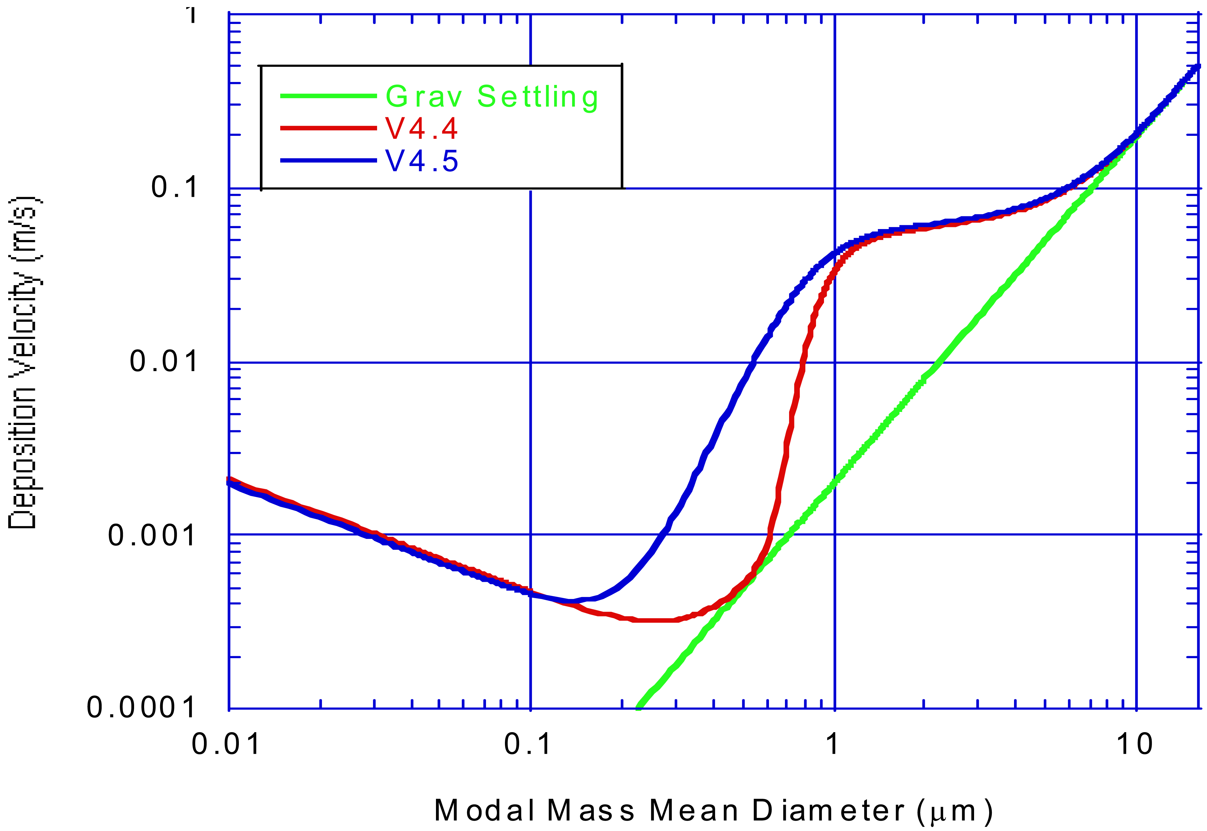
While turbulent flux through the atmospheric surface layer is similar for gases and aerosols, there are several key processes that are unique to aerosol dry deposition, including gravitational settling, Brownian diffusion, surface impaction, surface interception, and rebound. All of these processes are functions of particle diameter D_p, such that the dominant process depends on position in the particle size spectrum. For instance, Brownian diffusion dominates in the nano-range (D_p < 100 nm), where deposition efficiency increases with decreasing diameter, and gravitational settling and inertial impaction dominate in the super micron range, where their efficiencies increase with increasing diameter. Thus, there is a minimum of aerosol dry deposition velocity in the 0.1–1.0 μm range which is aptly named the accumulation range (e.g., see Figure 3). Recent reviews by Pryor et al. [94] and Petroff et al. [95] provide comprehensive literature surveys and overviews of modeling and measurements of aerosol dry deposition. Therefore, this section provides a description of the equations and techniques used for aerosol dry deposition calculations in the CMAQ model as an example of a state-of-the-science formulation in a widely used operational model.

To cast aerosol deposition in a resistance and velocity form, the simultaneous turbulent and sedimentation fluxes can be combined as derived by Venkatram and Pleim [96]:

$$V_d(D_p)=\frac{V_g}{1-exp\left(-V_g(R_a+R_b)\right)}$$

(16)

where the gravitational settling velocity is:

$$V_g=\frac{\mathit{\rho }{D}_p^2}{18\mathit{\mu }}{C}_c$$

(17)

ρ is the density of the aerosol, μ is air dynamic viscosity, and the Cunningham slip correction factor is:

$$C_c=1+\frac{\mathit{\lambda }}{D_p}\left[2.514+0.8e^{-0.55\frac{D_p}{\mathit{\lambda }}}\right]$$

(18)

where λ is the mean free path of air. Unlike gas deposition the quasi-laminar boundary layer resistance R_b is usually the limiting resistance for aerosols because Brownian diffusion is much slower for particles than molecular diffusion is for gases. However, the effects of inertial impaction and interception by protruding micro-scale roughness elements can partially bridge the diffusion layer such that R_b is inversely related to three collection efficiencies [97]:

$$R_b={\left[F_f{u}_{*}\left(S{c}^{-\stackrel{2}{}/\underset{3}{}}+E_{im}+E_{in}\right)\right]}^{-1}$$

(19)

where F_f is an empirical correction factor to account for increased deposition in convective conditions as suggested by Binkowski and Shankar [98]:

$$F_f=1+0.24\frac{{w_{*}}^2}{{u_{*}}^2}$$

(20)

where w_* is the convective velocity scale. The first term in Equation (19) represents the collection efficiency by diffusion across the quasi-laminar boundary layer, which is similar to Equation (8) for gasses except that the Schmidt number for aerosols is defined as Sc = v/D_B, where D_B is Brownian diffusivity which is a function of particle diameter. Slinn [97] suggested a formulation for the interception collection efficiency E_in that depends on the characteristic size of microscale structures such as tiny hairs on leaves and the characteristic size of the leaves. However, since it is difficult to specify realistic estimates of these parameters over the area of typical grid cells used by air quality models (i.e. ∼4–20 km) on the basis of available land use data the interception efficiency is not used in the CMAQ model.

Pryor [94] summarized many formulations for the impaction efficiency E_im and compares their magnitudes over a range of aerosol sizes. Slinn [99] suggested:

$$E_{im}={10}^{\stackrel{-3}{}/\underset{st}{}}$$

(21)

where Stokes number is:

$$St=\frac{V_g{u}_{*}^2}{g\mathit{\upsilon }}$$

(22)

Equation (21) was the form of E_im originally used in CMAQ. However, Slinn [97] noted that Equation (21) was derived from empirical fits to smooth surfaces and therefore may not be appropriate for complex canopies where there is a wide range of wind speeds and length scales of collectors (leaves). Thus, for vegetated surfaces, Slinn [97] recommended a form of E_im with weaker dependence on St:

$$E_{im}=\frac{S{t}^2}{c+S{t}^2}$$

(23)

This form of E_im was recently adopted for the CMAQ model, using the recommendation by Giorgi [100] that c = 400, so that aerosol deposition to heavily vegetated regions is better represented.

Air quality models that consider aerosol size distributions either by discrete size bins (sectional models) or by log-normal modes (modal models) compute aerosol dry deposition velocities as functions of particle diameter. Thus, for sectional models Equations (16–23) are evaluated using the mass mean diameter of each section. For modal models an integrated V_d is computed for each mode by integrating these equations over each log-normal size distribution as described by Binkowski and Shankar, [98] and Feng [101]. Figure 3 shows an example of modal integrated V_d as a function of modal mass mean diameter D_g and the results of the change in the impaction efficiency from Equation (21) that was used in CMAQv4.4 to the formulation shown by Equation (23) as used in CMAQv4.5 and later versions. This change in impaction efficiency has a profound effect on increasing the deposition velocity in the size range where the D_g for the accumulation mode typically resides.

3.3. Bidirectional Surface Flux Modeling

While most gas-phase atmospheric chemical constituents predominantly deposit to the surface (e.g.,O₃, SO₂, HNO₃) and some chemicals are predominantly emitted from the surface (e.g., isoprene and terpenes), a few chemicals such as ammonia, mercury, and certain oxidized VOCs exhibit distinctly bi-directional behavior where they alternately deposit and emit on diurnal, seasonal, or sometimes longer time-scales. Generally, air quality models include simultaneous emissions and dry deposition fluxes of these materials that are estimated using entirely unrelated techniques. This is clearly a less realistic treatment of the salient physical processes than a bi-directional gradient driven flux model that is responsive to changes at the model time step level. Thus, air quality modelers have recently been replacing separate representations of emissions and dry deposition with bi-directional flux calculations.

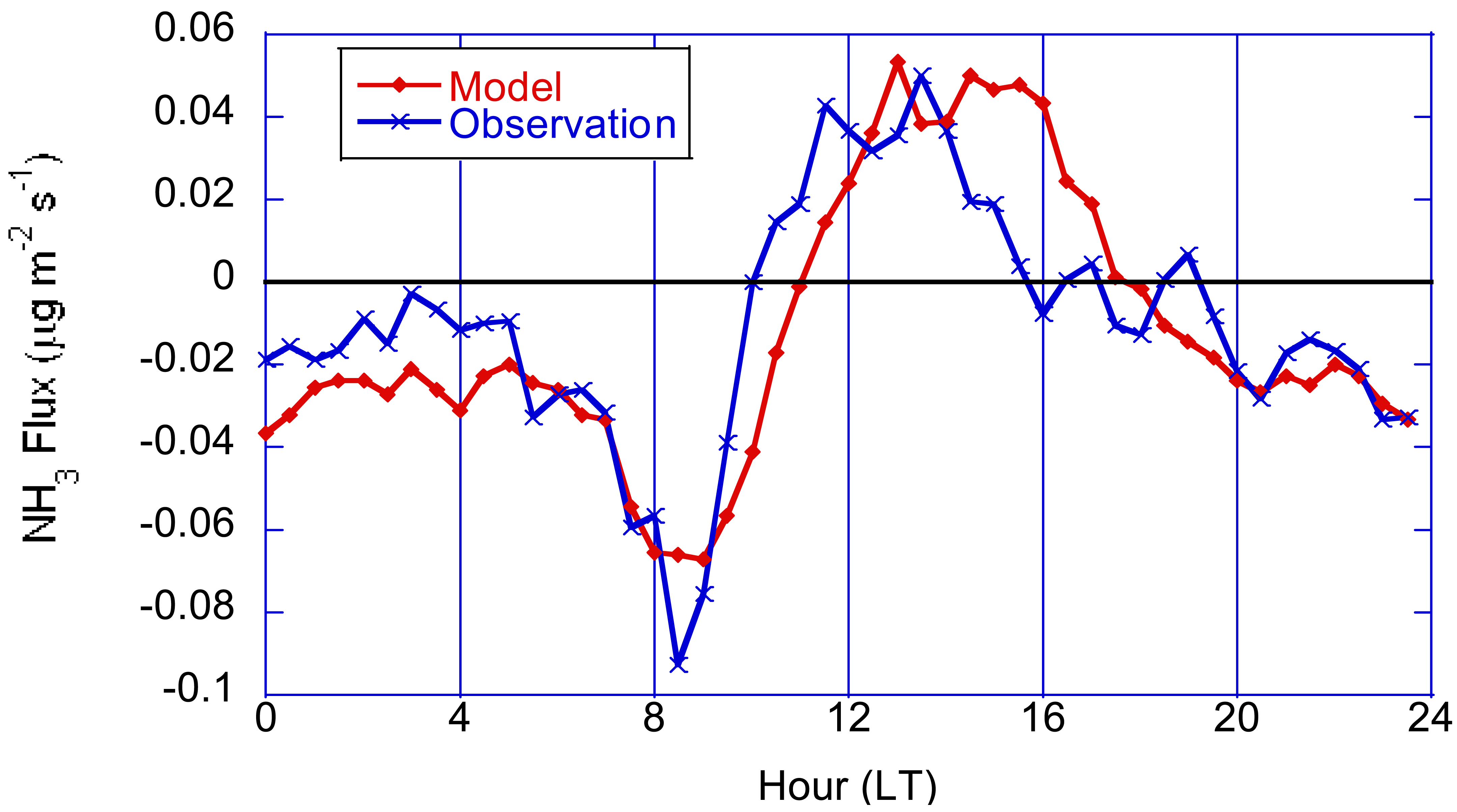
The development and application of bi-directional modeling of ammonia is particularly important since it allows for more accurate surface fluxes from fertilized fields which is a major contributor to excess nitrogen pollution that has adverse effects on human health, biodiversity, and climate change [18,22]. Ammonia fluxes can vary widely in magnitude and direction on spatial scales down to agricultural fields and temporally over diurnal, multi-day, and seasonal time-scales. In areas of unfertilized natural vegetation, ammonia flux is predominately deposition although small evasive fluxes can be driven by the thermodynamics of the equilibrium between ambient NH₃ and NH₄ in the leaf apoplastic solution when ambient concentrations are low and ambient temperatures are sufficiently high. Conversely, for heavily fertilized crops such as corn, ammonia fluxes are mostly upward (evasion), with the greatest fluxes immediately after fertilization and gradually decreasing over subsequent weeks and months. For minimally fertilized crops such as soybeans, fluxes can be truly bi-directional on a diurnal basis as shown in Figure 4 [26,102].

Sutton et al. [3] provided an extensive review of measurements and modeling techniques for ammonia surface exchange processes. In this section we outline the model for bi-directional flux modeling in the CMAQ modeling system developed initially following Sutton et al. [103] and Nemitz et al. [104] with further refinement through comparison to field study measurements in corn and soybean [102] fields. Personne et al. [105] and Burkhardt et al. [106] developed and evaluated similar bi-directional ammonia flux models in comparison to measurements in fertilized grassland during the GRAMINAE intensive measurement campaign in spring 2000 near Braunschweig, Germany.

Although bi-directional flux modeling has many commonalities with dry deposition modeling there are also important differences that stem from the complications of compensation concentrations in surface reservoirs. Hence, the simplicity of the linear flux-concentration relationship for dry deposition, which allows V_d to be computed for each chemical species upstream of the execution of the chemical transport model, is usually not feasible for bi-directional calculations because compensation points may differ for different pathways. For ammonia and mercury, compensation point concentrations are usually very different at the soil, stomata, and cuticle.

The total flux between the plant canopy and the overlying atmosphere is the sum of two bi-directional pathways, to the leaf stomata F_st and the soil F_g, and one uni-directional deposition pathway to the leaf cuticle F_cut (Figure 5). Because each bidirectional flux pathway depends on concentration difference across resistances, an in-canopy concentration χ_c is computed at the junction of the ground, stomatal, and cuticle pathways, which is often referred to as the net canopy compensation point [104]. Thus the total flux is defined as:

$$F_t=\frac{\left({\mathit{\chi }}_c-{\mathit{\chi }}_a\right)}{R_a}=F_g+F_{st}+F_{\mathit{\text{cut}}}$$

(24)

where χ_a is the concentration in the air above the canopy and the component fluxes are:

$$F_g=\frac{({\mathit{\chi }}_g-{\mathit{\chi }}_c)}{R_{ac}+R_{bg}+R_{\mathit{\text{soil}}}}$$

(25)

$$F_{st}=\frac{\left({\mathit{\chi }}_s-{\mathit{\chi }}_c\right)}{R_b+R_{st}}$$

(26)

$$F_{\mathit{\text{cut}}}=\frac{{\mathit{\chi }}_c}{R_b+R_w}$$

(27)

The resistances R_a, R_ac, R_b, and R_st are essentially the same as used for gas dry deposition with adjustments to R_b and R_st for molecular diffusivity. The resistances R_bg, R_soil, and R_w, however, required specific derivation for ammonia based on comparisons to field data and previous research described in the literature. In heavily fertilized fields ammonia concentrations in the soil can be extremely large, thus the parameterizations for R_bg and R_soil are critical for simulation of realistic fluxes from the soil. The cuticle resistance is also crucial since a large fraction of the soil flux can be absorbed by the leaves thereby greatly reducing the flux at the top of the canopy. A study by Bash et al. [107] using a combination of in-canopy concentration measurements, above-canopy flux measurements, and an analytical model, estimated that a corn canopy was a sink for up to 70% of ammonia emitted from the soil approximately one month following fertilization.

Air concentrations of ammonia in soil pores and stomatal cavities are assumed to be in Henry's Law equilibrium with aqueous concentrations of ammonium and hydrogen ion in the soil moisture and apoplast leaf tissue, respectively. Hence, the soil and stomatal compensation points (χ_g and χ_st) can be computed as [108]:

$${\mathit{\chi }}_{g,\mathit{\text{st}}}=\frac{A}{T_{g,st}}{10}^{-B/T_{g,st}}{\Gamma }_{\text{g},\text{st}}$$

(28)

where A (2.746 × 1015) and B (4507) are constants derived from the equlibria constants, T_g,st is the soil and leaf temperature (K), and Γ_g,st is the dimensionless NH₃ emission potential from the soil and leaf stomata where:

$$\Gamma =\frac{\left[N{H}_4^{+}\right]}{\left[H^{+}\right]}$$

(29)

Thus, ammonia bi-directional flux models depend on methodologies for estimating stomatal and soil gamma values for all land use and vegetation types. Zhang et al. [109] proposed a model where gamma values are specified according to land use category and season based on an extensive review of measurement studies. Massad et al. [5] proposed a more dynamic methodology for estimating gamma values, also based on extensive review of measurement studies, where Γ_st for unmanaged ecosystems is computed based on nitrogen input from deposition while for managed ecosystems Γ_g and Γ_st are functions of nitrogen fertilizer application with a decay function by time since fertilization. Cooter et al. [110] demonstrated that NH₃ flux from managed agricultural soils can be reasonably estimated by integrating the bi-directional resistance-based flux model in CMAQ with components of the Environmental Policy Integrated Climate (EPIC) model [111] to compute soil gamma values. Preliminary annual model simulations show improved estimates of NH_x wet deposition over the eastern US in general (reduction in mean error), with regions of significant bias reduction as well as regions of moderate increase in bias [112]. A more complete agricultural fertilizer modeling system that takes daily meteorological and nitrogen deposition data from WRF/CAMQ output and uses site, soil, crop, and management information to estimate fertilizer application method, timing, amount, and rate for specific pastures and crops on the model grid is being integrated with EPIC and CMAQ on a continental scale [113]. Future scenarios, such as increased bio-fuel production or climate change that may impact crop yields and fertilizer use, can be simulated with this system to assess their impacts on air quality.

Mercury is another important pollutant that exhibits strong bi-directional surface flux behavior. Unlike ammonia, however, the main source of surface mercury that volatilizes to the air is deposition from the air. Thus, bi-directional flux modeling is necessary to account for the hop-scotching of depositing and re-emitting mercury. Bash et al.[6] provided an overview of the processes and issues of bi-directional mercury exchange between the air and soil, vegetation, and surface waters. Zhang et al. [7] provided a review of measurements and modeling techniques. Bash [107] described a bi-directional elemental mercury exchange model that has been implemented and tested in the CMAQ system.

Semivolatile organic compounds (SOCs), such as polycyclic aromatic hydrocarbons (PAHs), polychlorinated biphenyls (PCBs), and other hazardous chemicals, transfer from air to the soil by particle or gas dry deposition and by wet deposition where they can accumulate over long periods of time [114]. If concentrations in soil become sufficiently high, these compounds can volatilize back to the air. In addition, residual organochlorine pesticides (OCPs), such DDT and Chlordane are still high enough in some agricultural soils to still be an atmospheric source [115]. Air-surface exchange of SOCs is modeled by estimation of equilibrium partitioning with bi-directional fluxes controlled by deviations from the equilibrium state [116].

4. Recent Advances in Chemical Surface Flux Modeling

In the early 1980s, two comprehensive reviews of gas and particle dry deposition were published by Hosker and Lindberg [117] and Sehmel [118]. Later, Wesely and Hicks [119], reviewed the state of knowledge on dry deposition. At that time the major processes controlling the deposition of the major inorganic species such as SO₂, O₃ were well understood because of the relative abundance of flux measurement studies of these species. For example, many flux measurements, mostly of ozone but also some of SO₂ and NO₂, have been made by gradient and eddy correlation methods going back several decades, starting in the 1970s [120,121], with many more in the 1980s and 1990s [122–126]. Note that reliable eddy correlation measurements over forest canopies were not feasible until the 1990s [127–129]. Because of the extensive measurement data in the published record the modeling of these species has been somewhat constrained. Significant improvements in the modeling gas dry deposition in recent years have resulted from advances in land surface modeling and closer coupling between air quality and meteorology models. Since stomatal resistance, aerodynamic resistance, quasi-laminar boundary layer resistance, surface and canopy wetness, and snow cover are important parameters for both latent heat flux and dry deposition of many gases, air quality modeling systems that are comprised of meteorology and chemical transport models, such as the WRF-CMAQ system, can use the same parameters for both dry deposition and land surface modeling [25].

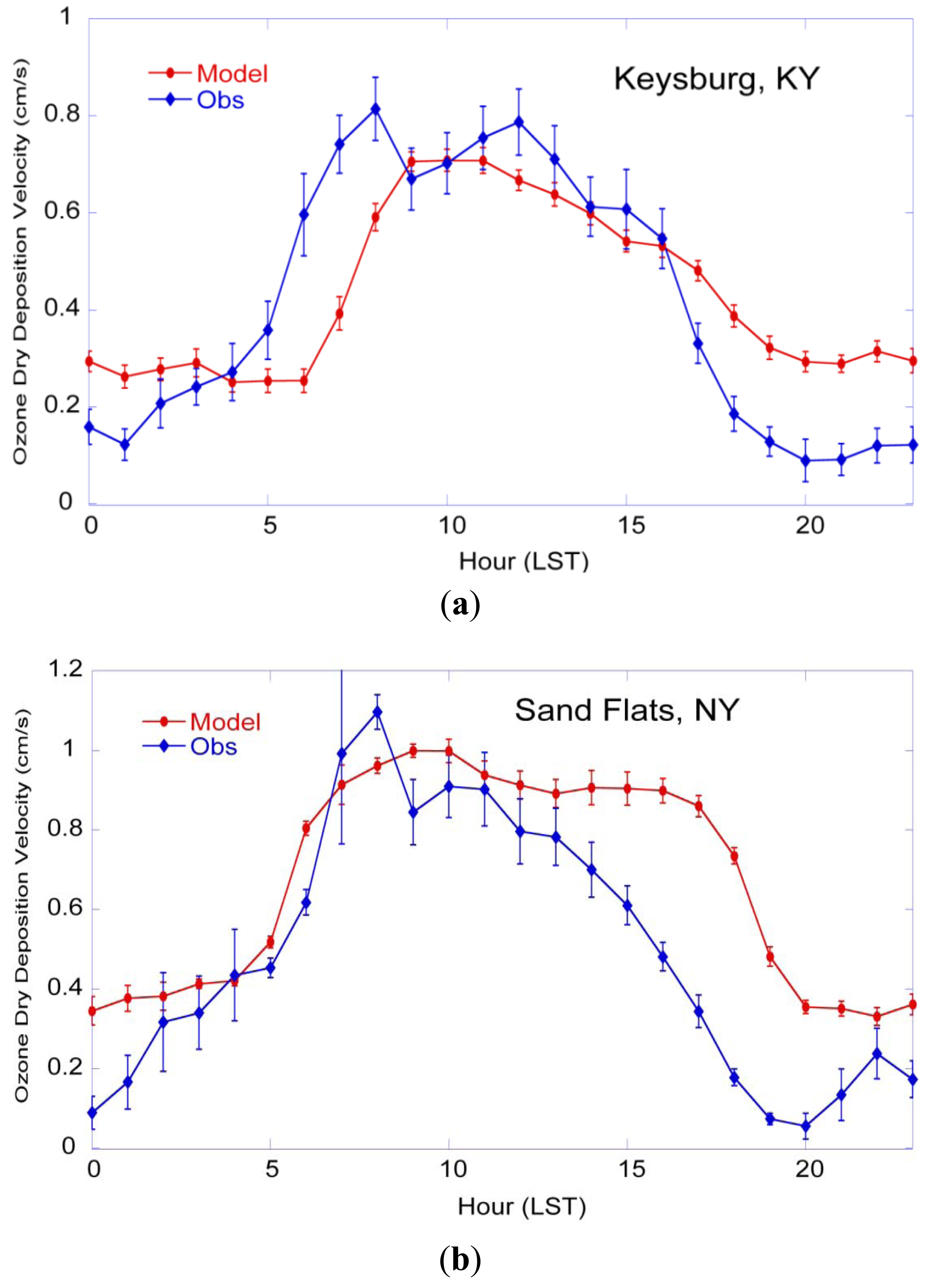
Examination of dry deposition velocities modeled by CMAQ along with concurrent parameters from the LSM in WRF demonstrates the close relationships between these processes. Figure 6 shows ozone dry deposition on a 12 km grid simulated by CMAQ for a summer afternoon (19 UT), which is within the range usually measured in the field with peak values of about 1.1 cm/s. The spatial pattern illustrates that ozone deposits primarily through the stomatal pathway since the highest values are in the most vegetated areas. It is interesting that high deposition velocities are simulated for both heavily forested areas in the East and agricultural areas in the Midwest because forests generally have higher LAI than crops but crops have much lower minimum stomatal resistance. Thus, ozone dry deposition velocity closely follows the latent heat flux (Figure 7) except where there is evaporation from rain wetted canopies. Note, however, that there is some enhancement of V_d for wet canopies (e.g., in southern Quebec) because the cuticular resistance for ozone is set to a lower value than would result from Henry's law scaling (also lower than dry cuticular resistance) on the basis of a study comparing measured ozone flux and latent heat flux [2]. CMAQ's dry deposition model has been evaluated through comparison to measurements over soybeans in Kentucky and mixed forest in upstate NY [130] as shown in Figure 8. While there is some lag in the morning increase of V_d for the soybeans, and overprediction at night, the gradual afternoon decline which is caused by stomatal response to lower RH is well represented.

The dry deposition velocity for SO₂ is far more influenced by surface wetness as shown in Figure 2a because of its high effective Henry's law solubility. The highest values of V_d for SO₂ are all in the same areas where LE is high from evaporating surface wetness (see also Figure 2b). In these areas, where rain is occurring currently or recently, peak values are 3–4 cm/s, which indicates that there is very little surface resistance in these areas. Dry deposition of NO₂ and NO were studied in relationship to O₃ and ET in a series of gas exchange experiments involving tobacco and sunflower plants described by Neubert et al. [131]. These experiments showed that NO₂ deposition is almost entirely stomatal with negligible mesophyll resistance, while NO had considerable mesophyll resistance that changed with light intensity. These experiments also showed that ozone deposition occurs by stomatal uptake with negligible mesophyll resistance and destruction at cuticle surfaces. A field measurement study of PAN fluxes over grassland by Doskey et al.[67] found that PAN deposition is mostly via the stomatal pathway but with a non-zero mesophyll resistance resulting in V_d values 0.5−0.3 of V_d for O₃, which is in concurrence with previous studies. However, leaf level measurements reported by Sparks et al. [132] suggest unimpeded stomatal uptake of PAN, indicating insignificant mesophyll resistance and higher deposition velocities. Furthermore, recent eddy covariance flux measurements over loblolly pine by Turnipseed et al. [133] show total surface conductance about twice the stomatal conductance, which suggests significant cuticular uptake. On the basis of these measurement studies the CMAQ was revised in 2007 with higher values of surface reactivity scaling parameter for PAN resulting in maximum deposition velocities close to the values for O₃.

Recently, many more chemical species are being added to dry deposition models as measurement techniques improve in detection capability and response time and the needs of the modeling community extend to more environmental issues such as air toxics and ecosystem impacts. For example, many toxic gases have been added to the CMAQ model in recent years, thereby requiring estimates of dry deposition velocity for these chemicals. However, the lipid solubility scaling discussed in Section 3 has yet to be applied to the CMAQ dry deposition model. A recent study by Karl et al. [134] promotes the importance of the dry deposition of oxygenated VOCs, many of which are oxidation products of biogenic VOCs. They found that Methyl vinyl ketone (MVK) and Methacrolin (MAC), which account for about 80% of the initial oxidation products of isoprene, have deposition velocities of similar magnitude as O₃. On the basis of this study CMAQ is being updated to include dry deposition of MVK and MAC. The dry deposition model in AURAMS described by Zhang et al.[46] already includes dry deposition of these species although with small values of V_d than suggested by Karl et al. [134].

5. Conclusions

Modeling of surface fluxes for air quality modeling involves micrometeorology, plant physiology and biology, surface chemistry, soil hydraulics and physics, agricultural management, spatial descriptions of geophysical characteristics, and most importantly, surface flux measurements for a variety of chemical substances over a variety of landscapes. Uncertainties in parameterizations, incomplete knowledge of processes, limitations to theory, and paucity of detailed data and measurements, combine to limit the realism and accuracy of surface flux models used in large-scale (mesoscale to global) air quality modeling systems. Progress is being made on many of these fronts but significant uncertainties remain. Even for ozone dry deposition, which is the most widely measured substance, current model results still show substantial errors compared to observations (Figure 8). Some of the errors in chemical fluxes have their source in common with the meteorological fluxes (heat, moisture, and momentum), such as the aerodynamic resistance, while other errors are due to incomplete understanding of chemical interactions with surfaces and leaf tissue. Further errors can be attributed to insufficient detail and accuracy in the spatial and temporal representations of landscape, land use, and vegetation in meso to global scale grid models.

Surface flux modeling relies on flux-profile relationships in accordance with Monin-Obukov similarity theory (MOST) in the atmospheric surface layer [135] (Equation 1). The MOST relationships are defined by dimensionless universal profile functions that have been empirically determined from the 1968 KANSAS experiment [136]. Thus, the validity of MOST is limited to flat terrain with uniform landscape and landcover [137]. Not only are MOST-based model calculations less accurate in non-ideal conditions, but also flux measurements are generally unreliable in complex landscapes. For substances that are mainly limited by surface resistances (e.g., O₃, NO₂, PAN), the limitation of MOST and resulting inaccuracies in estimates of R_a in non-ideal conditions such as sloping terrain or patchy land-use will have relatively small effects on V_d calculations [119]. However, for species not limited by surface uptake, such as HNO₃ or other highly soluble species such as H2O₂ or SO₂ when surfaces are wet, V_d estimates should be considered especially suspect in hilly or patchy landscapes.

There are distinct advantages to an integrated or coupled approach to LSM and chemical flux modeling. As meteorology and air quality models become more integrated such as, WRF-Chem [138], WRF-CMAQ [139], COSMO-ART [140], GATOR [141], to name a few, there is more opportunity for integrated surface flux algorithms that share key parameters like R_a, R_st, and R_b between meteorological and chemical flux models. Such integrated approaches not only ensure consistency but also potentially benefit the chemical flux calculations by using a more realistic stomatal conductance estimates from the ET modeling in the meteorological LSM. For example, in the WRF-CMAQ system the latent heat flux is optimized by an indirect soil moisture data assimilation scheme that effectively tunes the stomatal conductance through its dependence on soil moisture [41]. Thus, the resulting stomatal conductance is more constrained and generally more accurate than estimates by stand-alone dry deposition models. In this way, chemical flux models and air quality models automatically benefit as land surface models are improved.

Advancements in land surface and chemical surface flux modeling will depend on improved descriptions of land use and vegetation characteristics. For example, high resolution land use and land cover data from the NLCD, based on 30 m resolution LANDSAT thematic mapper, have recently been incorporated into the WRF-CMAQ system for land surface and chemical flux modeling [142]. Furthermore, a more detailed vegetation dataset is being developed by combining the high spatial resolution land use data from NLCD with county-level tree species data from the Forest Inventory Analysis (FIA) and crop data from the National Agricultural Statistical Service (NASS) [113]. By combining with ecoregion information this dataset will be able to better define key parameters such as minimum stomatal conductance, LAI, and canopy height across continental gridded modeling domains. Ultimately, the same data set with high spatial and vegetation-type resolution will be used for chemical surface fluxes, meteorological land surface modeling, and biogenic emissions.

Chemical, meteorological, and hydrological surface fluxes are key interface processes that link the atmosphere to the terrestrial, aquatic, and marine components of the Earth system. The dry deposition components of air quality models are expanding in scope to include many more chemical species that are important not only for atmospheric constituents but also as inputs to terrestrial and aquatic ecosystems. In addition, there is growing interest in the deposition of toxic contaminants that enter the food chain via air-surface exchange and subsequently impact human health. There has also been an extension to modeling substances that have surface compensation points (e.g., ammonia and mercury) necessitating the development of bi-directional flux capability. The new bi-directional systems often require adjunct land models such as agricultural management models (e.g., EPIC) that are used for ammonia from fertilizer. All of these extensions to the traditional dry deposition models urgently need evaluation and constraint from field and laboratory measurements.

References

- Massman, W.J.; Grantz, D.A. Estimating canopy conductance to ozone uptake from observations of evapotranspiration at the canopy scale and at the leaf scale. Glob. Chang. Biol. 1995, 1, 183–198. [Google Scholar]
- Pleim, J.E.; Finkelstein, P.L.; Clarke, J.F.; Ellestad, T.G. A Technique for Estimating Dry Deposition Velocities Based on Similarity with Latent Heat Flux. Atmos. Environ. 1999, 33, 2257–2268. [Google Scholar]
- Sutton, M.A.; Nemitz, E.; Erisman, J.W.; Beier, C.; Butterbach Bahl, K.; Cellier, C.; de Vries, W.; Cotrufo, F.; Skiba, U.; Di Marco, C.; et al. Challenges in quantifying biosphere atmosphere exchange of nitrogen species. Environ. Pollut. 2007, 150, 125–139. [Google Scholar]
- Kruit, R.J.W.; van Pul, W.A.J.; Sauter, F.J.; van den Broek, M.; Nemitz, E.; Sutton, M.A.; Krol, M.; Holtslag, A.A.M. Modeling the surface-atmosphere exchange of ammonia. Atmos. Environ. 2010, 44, 945–957. [Google Scholar]
- Massad, R.S.; Nemitz, E.; Sutton, M.A. Review and parameterization of bi-directional ammonia exchange between vegetation and the atmosphere. Atmos. Chem. Phys. 2010, 10, 10359–10386. [Google Scholar]
- Bash, J.O.; Bresnahan, P.; Miller, D.R. Dynamic surface interface exchanges of mercury: A review and compartmentalized modeling framework. J. Appl. Meteorol. Climatol. 2007, 46, 1606–1618. [Google Scholar]
- Zhang, L.; Wright, L.P.; Blanchard, P. A review of current knowledge concerning dry deposition of atmospheric mercury. Atmos. Environ. 2009, 43, 5853–5864. [Google Scholar]
- Ganzeveld, L.; Eerdekens, G.; Feig, G.; Fischer, H.; Harder, H.; Königstedt, R.; Kubistin, D.; Martinez, M.; Meixner, F.X.; Scheeren, H.A.; et al. Surface and boundary layer exchanges of volatile organic compounds, nitrogen oxides and ozone during the GABRIEL campaign. Atmos. Chem. Phys. 2008, 8, 6223–6243. [Google Scholar]
- Guenther, A.; Karl, T.; Harley, P.; Wiedinmyer, C.; Palmer, P.I.; Geron, C. Estimates of global terrestrial isoprene emissions using MEGAN (Model of Emissions of Gases and Aerosols from Nature). Atmos. Chem. Phys. 2006, 6, 3181–3210. [Google Scholar]
- Karlsson, P.E.; Uddling, J.; Braun, S.; Broadmeadow, M.; Elvira, S.; Gimeno, B.S.; Le Thiec, D.; Oksanen, E.; Vandermeiren, K.; Wilkinson, M.; et al. New critical levels for ozone impact on trees based on leaf cumulated ozone uptake. Atmos. Environ. 2004, 38, 2283–2294. [Google Scholar]
- Emberson, L.D.; Buker, P.; Ashmore, M.R. Assessing the risk caused by ground level ozone to European forest trees: A case study in pine, beech and oak across different climate regions. Environ. Pollut. 2007, 147, 454–466. [Google Scholar]
- Tuovinen, J.-P.; Emberson, L.; Simpson, D. Modelling ozone fluxes to forests for risk assessment: status and prospects. Ann. For. Sci. 2009, 66, 401. [Google Scholar]
- Musselman, R.C.; Massman, W.J. Ozone flux to vegetation and its relationship to plant response and ambient air quality standards. Atmos. Environ. 1999, 33, 65–73. [Google Scholar]
- EPA. Policy Assessment for the Review of the Secondary National Ambient Air Quality Standards for Oxides of Nitrogen and Oxides of Sulfur; EPA-452/R-11-005a; U.S. Environmental Protection Agency: Research Triangle Park, CA, USA, 2011; p. 364. [Google Scholar]
- Byun, D.; Schere, K.L. Review of the governing equations, computational algorithms, and other components of the Models-3 Community Multiscale Air Quality (CMAQ) modeling system. Appl. Mech. Rev. 2006, 59, 51–77. [Google Scholar]
- Galloway, J.N. An Earth-system perspective of the global nitrogen cycle. Nature 2008, 451, 293–296. [Google Scholar]
- Millennium Ecosystem Assessment (MA). Ecosystems and Human Well-being: Synthesis; Island Press: Washington, DC, USA, 2005. Available online: http://www.millenniumassessment.org/en/Synthesis.aspx (accessed on 31 May 2011).
- Erisman, J.W.; Sutton, M.A.; Galloway, J.; Klimont, Z.; Winiwarter, W. How a century of ammonia synthesis changed the world. Nat. Geosci. 2008, 1, 636–639. [Google Scholar]
- Smith, V.H.; Tilman, G.D.; Nekola, J.C. Eutrophication: Impacts of excess nutrient inputs on freshwater, marine, and terrestrial ecosystems. Environ. Pollut. 1998, 100, 179–196. [Google Scholar]
- Boyer, E.W.; Goodale, C.L.; Jaworski, N.A.; Howarth, R.W. Anthropogenic nitrogen sources and relationships to riverine nitrogen export in the northeastern USA. Biogeochemistry 2002, 57–58,, 137–169. [Google Scholar]
- Lovett, G.M.; Tear, T.H.; Evers, D.C.; Findlay, S.E.G.; Cosby, B.J.; Dunscomb, J.K.; Driscoll, C.T.; Weathers, K.C. Effects of air pollution on ecosystems and biological diversity in the eastern United States. Ann. N. Y. Acad. Sci. 2009, 1162, 99–135. [Google Scholar]
- Sutton, M.A.; Oenema, O.; Erisman, J.W.; Leip, A.; van Grinsven, H.; Winiwarter, W. Too much of a good thing. Nature 2011, 472, 159–161. [Google Scholar]
- Pleim, J.E.; Xiu, A. Development and testing of a surface flux and planetary boundary layer model for application in mesoscale models. J. Appl. Meteorol. 1995, 34, 16–32. [Google Scholar]
- Xiu, A.; Pleim, J.E. Development of a land surface model. Part I: Application in a mesoscale meteorological model. J. Appl. Meteorol. 2001, 40, 192–209. [Google Scholar]
- Pleim, J.E.; Xiu, A.; Finkelstein, P.L.; Otte, T.L. A coupled land surface and dry deposition model and comparison to field measurements of surface heat, moisture, and ozone fluxes. Water Air Soil Pollut. Focus 2001, 1, 243–252. [Google Scholar]
- Pleim, J.E.; Walker, J.; Bash, J.; Cooter, E. Development and Evaluation of an Ammonia Bi-Directional Flux Model for Air Quality Models. In Air Pollution Modeling and Its Applications XXI; Steyn, D.G., Castelli, S.T., Eds.; Springer Science + Business Media B.V.: Dordrecht, The Netherlands, 2011; in press. [Google Scholar]
- Skamarock, W.C.; Klemp, J.B.; Dudhia, J.; Gill, D.O.; Barker, D.M.; Powers, J.G. A description of the advanced research WRF version 3. Atmos. Res. 2008, 468, 113. [Google Scholar]
- Wesely, M.L.; Hicks, B.B. Some factors that affect the deposition rates of sulfur dioxide and similar gases on vegetation. J. Air Pollut. Control Assoc. 1977, 27, 1110–1116. [Google Scholar]
- Garratt, J.R.; Hicks, B.B. Momentum, heat and water vapour transfer to and from natural and artificial surfaces. Q. J. R. Meteorol. Soc. 1973, 99, 680–687. [Google Scholar]
- Dollard, G.J.; Atkins, D.H.F.; Davies, T.J.; Healy, C. Concentrations and dry deposition velocities of nitric acid. Nature 1987, 326, 481–483. [Google Scholar]
- Huebert, B.J.; Robert, C.H. The dry deposition of nitric acid to grass. J. Geophys. Res. 1985, 90, 2085–2090. [Google Scholar]
- Meyers, T.P.; Finkelstein, P.L.; Clarke, J.; Ellestad, T.G.; Sims, P.F. A multi-layer model for inferring dry deposition using standard meteorological measurements. J. Geophys. Res. 1998, 103, 22645–22661. [Google Scholar]
- Wu, Y.; Brashers, B.; Finkelstein, P.L.; Pleim, J.E. A multilayer biochemical dry deposition model, 1. Model formulation. J. Geophys. Res. 2003, 108, 4013. [Google Scholar]
- Erisman, J.W.; van Pul, A.; Wyers, P. Parameterization of dry deposition mechanisms for the quantification of atmospheric input to ecosystems. Atmos. Environ. 1994, 28, 2595–2607. [Google Scholar]
- Zhang, L.; Brook, J.; Vet, R. A revised parameterization for gaseous dry deposition in air-quality models. Atmos. Chem. Phys. 2003, 3, 2067–2082. [Google Scholar]
- Jarvis, P.G. The interpretation of leaf water potential and stomatal conductance found in canopies in the field. Phil. Trans. R. Soc. Lond. B 1976, 273, 593–610. [Google Scholar]
- Cowan, I.R. Stomatal Behaviour and Environment. Adv. Bot. Res. 1978, 4, 117–228. [Google Scholar]
- Farquhar, G.D.; Caemmerer, S.V.; Berry, J.A. A biochemical-model of photosynthetic CO2 assimilation in leaves of C-3 species. Planta 1980, 149, 78–90. [Google Scholar]
- Ball, J.; Woodrow, I.; Berry, J. A model predicting stomatal conductance and its contribution to the control of photosynthesis under different environmental conditions. Prog. Photosynth. Res. 1987, 4, 221–224. [Google Scholar]
- Leuning, R. A critical appraisal of a combined stomatal-photosynthesis model for C3 plants. Plant Cell Environ. 1995, 18, 339–355. [Google Scholar]
- Pleim, J.E.; Xiu, A. Development of a land surface model. Part II: Data assimilation. J. Appl. Meteorol.Climatol. 2003, 42, 1811–1822. [Google Scholar]
- Jacquemin, B.; Noilhan, J. Sensitivity study and validation of a land surface parameterization using the HAPEX-MOBILHY data set. Bound.-Layer Meteorol. 1990, 52, 93–134. [Google Scholar]
- Noilhan, J.; Planton, S. A simple parameterization of land surface processes for meteorological models. Mon. Weather Rev. 1989, 117, 536–549. [Google Scholar]
- Chen, F.; Dudhia, J. Coupling an advanced land-surface—hydrology model with the Penn State/NCAR MM5 modeling system. Part I: Model implementation and sensitivity. Mon. Weather Rev. 2001, 129, 569–604. [Google Scholar]
- Hicks, B.B.; Baldocchi, D.D.; Meyers, T.P.; Hosker, R.P., Jr.; Matt, D.R. A preliminary multiple resistance routine for deriving dry deposition velocities from measured quantities. Water Air Soil Pollut. 1987, 36, 311–330. [Google Scholar]
- Zhang, L.; Moran, M.; Makar, P.; Brook, J.; Gong, S. Modelling Gaseous Dry Deposition in AURAMS A Unified Regional Air-quality Modelling System. Atmos. Environ. 2002, 36, 537–560. [Google Scholar]
- Collatz, J.; Ball, J.; Grivet, C.; Berry, J. Physiological and environmental regulation of stomatal conductance, photosynthesis and transpiration: A model that includes a laminar boundary layer. Agric. For. Meteorol. 1991, 54, 107–136. [Google Scholar]
- Sellers, P.J.; Randall, D.A.; Collatz, G.J.; Berry, J.A.; Field, C.B.; Dazlich, D.A.; Zhang, C.; Collelo, G.D.; Bounoua, L. A revised land surface parameterization (SiB2) for atmospheric GCMs. Part I: Model formulation. J. Clim. 1996, 9, 676–705. [Google Scholar]
- Cox, P.; Betts, R.; Bunton, C.; Essery, R.; Rowntree, P.; Smith, J. The impact of new land surface physics on the GCM simulation of climate and climate sensitivity. Clim. Dyn. 1999, 15, 183–203. [Google Scholar]
- Bonan, G.B.; Lawrence, P.J.; Oleson, K.W.; Levis, S.; Jung, M.; Reichstein, M.; Lawrence, D.M.; Swenson, S.C. Improving canopy processes in the Community Land Model version 4 (CLM 4) using global flux fields empirically inferred from FLUXNET data. J. Geophys. Res. 2011, 116, G02014. [Google Scholar]
- Zaehle, S.; Friend, A.D. Carbon and nitrogen cycle dynamics in the O–CN land surface model: 1. Model description, site-scale evaluation, and sensitivity to parameter estimates. Glob. Biogeochem. Cycles 2010, 24, GB1005. [Google Scholar]
- Lohammar, T.; Larsen, S.; Linder, S.; Falk, S.O. FAST-simulation models of gaseous exchange in Scots pine. In Structure and Function of Northern Coniferous Forests: An Ecosystem Study; Persson, T., Ed.; Ecological Bulletin No. 32; Swedish Natural Science Research Council: Stockholm, The Netherlands, 1980; pp. 505–523. [Google Scholar]
- Monteith, J.L. A reinterpretation of stomatal responses to humidity. Plant Cell Environ. 1995, 18, 357–364. [Google Scholar]
- Aphalo, P.J.; Jarvis, P.G. Do stomata respond to relative humidity? Plant Cell Environ. 1993, 14, 127–132. [Google Scholar]
- Pleim, J.E. Modeling stomatal response to atmospheric humidity. In Preprints, 13th Symp. on Boundary Layers and Turbulence; American Meteorological Society: Boston, MA, USA, 1999; pp. 291–294. [Google Scholar]
- Gibelin, A.L.; Calvet, J.C.; Roujean, J.L.; Jarlan, L.; Los, S. Ability of the land surface model ISBA-A-gs to simulate leaf area index at the global scale: Comparison with satellites products. J. Geophys. Res. 2006, 111, D18102. [Google Scholar]
- Wu, Z.; Wang, X.; Chen, F.; Turnipseed, A.A.; Guenther, A.B.; Niyogi, D.; Charusombat, U.; Xia, B.; Munger, J.W.; Alapaty, K. Evaluating the calculated dry deposition velocities of reactive nitrogen oxides and ozone from two community models over a temperate deciduous forest. Atmos. Environ. 2011, 45, 2663–2674. [Google Scholar]
- Niyogi, D.S.; Alapaty, K.; Raman, S.; Chen, F. Development and evaluation of a coupled photosynthesis-based gas exchange evapotranspiration model, GEM for mesoscale weather forecasting applications. J. Appl. Meteorol. Climatol. 2009, 48, 349–368. [Google Scholar]
- Hirabayashi, S.; Kroll, C.N.; Nowak, D.J. Component-based development and sensitivity analyses of an air pollutant dry deposition model. Environ. Model. Softw. 2011, 26, 804–816. [Google Scholar]
- Pleim, J.; Venkatram, A.; Yamartino, R. ADOM/TADAP Model Development Program: The Dry Deposition Module; Ontario Ministry of the Environment: Rexdale, Canada, 1984; Volume 4. [Google Scholar]
- Padro, J.; den Hartog, G.; Neumann, H.H. An investigation of the ADOM dry deposition module using summertime O3 measurements above a deciduous forest. Atmos. Environ. 1991, 25, 1689–1704. [Google Scholar]
- Walcek, C.J.; Brost, R.A.; Chang, J.S.; Wesely, M.L. SO2, sulfate and HNO3 deposition velocities computed using regional landuse and meteorological data. Atmos. Environ. 1986, 20, 949–964. [Google Scholar]
- Smith, R.I.; Fowler, D.; Sutton, M.A.; Flechard, C.; Coyle, M. Regional estimation of pollutant gas dry deposition in the UK: model description, sensitivity analyses and outputs. Atmos. Environ. 2000, 34, 3757–3777. [Google Scholar]
- Ganzeveld, L.; Lelieveld, J. Dry deposition parameterization in a chemistry general circulation model and its influence on the distribution of reactive trace gases. J. Geophys Res. 1995, 100, 20999–21012. [Google Scholar]
- Wesely, M.L. Parameterization of surface resistances to gaseous dry deposition in regional-scale numerical models. Atmos. Environ. 1989, 23, 1293–1304. [Google Scholar]
- Jones, M.R.; Leith, I.D.; Fowler, D.; Raven, J.A.; Sutton, M.A.; Nemitz, E.; Cape, J.N.; Sheppard, L.J.; Smith, R.I.; Theobald, M.R. Concentration-dependent NH3 deposition processes for mixed moorland semi-natural vegetation. Atmos. Environ. 2007, 41, 2049–2060. [Google Scholar]
- Doskey, P.V.; Kotamarthi, V.R.; Fukui, Y.; Cook, D.R.; Breitbeil, F.W., III; Wesely, M.L. Air-surface exchange of peroxyacetyl nitrate at a grassland site. J. Geophys. Res. 2004, 109, D10310. [Google Scholar]
- Barbera, J.L.; Thomas, G.O.; Kerstiens, G.; Jones, K.C. Current issues and uncertainties in the measurement and modeling of air-vegetation exchange and within-plant processing of POPs. Environ. Pollut. 2004, 128, 99–138. [Google Scholar]
- Baldocchi, D.D. Deposition of Gaseous Sulfur Compounds to Vegetation. In Sulfur Nutrition and Assimilation in Higher Plants: Physiological Functions and Environmental Significances; De Kok, L.J., Stulen, I., Rennenberg, H., Brunold, C., Rauser, W.E., Eds.; SPB Academic Publishing: The Hague, The Netherlands, 1993; pp. 271–294. [Google Scholar]
- Helmig, D.; Bocquet, F.; Cohen, L.; Oltmans, S.J. Ozone uptake to the polar snow at Summit, Greenland. Atmos. Environ. 2007, 41, 5061–5076. [Google Scholar]
- Stocker, D.W.; Zeller, K.F.; Stedman, D.H. O3 and NO2 Fluxes over snow measured by eddy correlation. Atmos. Environ. 1995, 29, 1299–1305. [Google Scholar]
- Galbally, I.; Allison, I. Ozone fluxes over snow surfaces. J. Geophys. Res. 1972, 77, 3946–3949. [Google Scholar]
- Colbeck, I.; Harrison, R.H. Dry deposition of ozone: some measurements of deposition velocity and of vertical profiles to 100 meters. Atmos. Environ. 1985, 19, 1807–1818. [Google Scholar]
- Padro, J.; Neumann, H.H.; Den Hartog, G. Modeled and observed dry deposition velocity of O3 above a deciduous forest in the winter. Atmos. Environ. 1992, 26A, 775–784. [Google Scholar]
- Hopper, J.F.; Barrie, L.A.; Silis, A.; Hart, W.; Gallant, A.J.; Dryfhout, H. Ozone and meteorology during the 1994 polar Sunrise Experiment. J. Geophys. Res. 1998, 103, 1481–1492. [Google Scholar]
- Aldaz, L. Flux measurements of atmospheric ozone over land and water. J. Geophys. Res. 1969, 74, 6943–6946. [Google Scholar]
- Bales, R.; Valdez, M.; Dawson, G. Gaseous deposition to snow 2. Physical-chemical model for SO2 deposition. J. Geophys. Res. 1987, 92, 9789–9799. [Google Scholar]
- Whisler, F.D.; Acock, B.; Baker, D.N.; Fye, R.E.; Hodges, H.F.; Lambert, J.R.; Reddy, R. Crop simulation models in agronomic systems. Adv. Agron. 1986, 40, 141–208. [Google Scholar]
- de Pury, D.G.G.; Farquhar, G.D. Simple scaling of photosynthesis from leaves to canopies without the errors of big-leaf models. Plant Cell Environ. 1997, 20, 537–557. [Google Scholar]
- Zhang, L.; Moran, M.D.; Brook, J.R. A comparison of models to estimate in-canopy photosynthetically active radiation and their influence on canopy stomatal resistance. Atmos. Environ. 2001, 35, 4463–4470. [Google Scholar]
- Walko, R.L. Coauthors, coupled atmosphere-biophysics-hydrology models for environmental modeling. J. Appl. Meteorol. 2000, 39, 931–944. [Google Scholar]
- Dickinson, R.E.; Henderson-Sellers, A.; Kennedy, P.J. Biosphere-Atmosphere Transfer Scheme (BATS) version 1e as coupled to the NCAR Community Climate Model; Tech. Note NCAR/ TN-378+STR; National Center for Atmospheric Research: Boulder, CO, USA, 1993; p. 72. [Google Scholar]
- Lawrence, P.J.; Chase, T.N. Representing a new MODIS consistent land surface in the Community Land Model (CLM 3.0). J. Geophys. Res. 2007, 112, G01023. [Google Scholar]
- Moore, N.; Torbick, N.; Lofgren, B.; Wang, J.; Pijanowski, B.; Andresen, J.; Kim, D.-Y.; Olson, J. Adapting MODIS-derived LAI and fractional cover into the RAMS in East Africa. Int. J. Clim. 2010, 30, 1954–1969. [Google Scholar]
- Buermann, W.; Dong, J.; Zeng, X.; Myneni, R.B.; Dickinson, R.E. Evaluation of the Utility of Satellite-Based Vegetation Leaf Area Index Data for Climate Simulations. J. Clim. 2001, 14, 3536–3550. [Google Scholar]
- Masson, V.; Champeaux, J.-L.; Chauvin, F.; Meriguet, C.; Lacaze, R. A global database of land surface parameters at 1-km resolution in meteorological and climate models. J. Clim. 2003, 16, 1261–1282. [Google Scholar]
- Rodell, M.; Houser, P.R.; Jambor, U.; Gottschalck, J.; Mitchell, K.; Meng, C.-J.; Arsenault, K.; Cosgrove, B.; Radakovich, J.; Bosilovich, M.; et al. The global land data assimilation system. Bull. Am. Meteorol. Soc. 2004, 85, 381–394. [Google Scholar]
- Huete, A.; Didan, K.; Miura, T.; Rodriguez, E.P.; Gao, X.; Ferreira, L.G. Overview of the radiometric and biophysical performance of the modis vegetation indices. Remote Sens. Environ. 2002, 83, 195–213. [Google Scholar]
- Zhang, X.; Friedl, M.A.; Schaaf, C.B.; Strahler, A.H. Climate controls on vegetation phenological patterns in northern mid-and high latitudes inferred from MODIS data. Glob. Chang. Biol. 2004, 10, 1–13. [Google Scholar]
- Nagler, P.; Glenn, E.; Thompson, T.; Huete, A. Leaf area index and normalized difference vegetation index as predictors of canopy characteristics and light interception by riparian species on the lower colorado river. Agric. For. Meteorol. 2004, 125, 1–17. [Google Scholar]
- Glenn, E.P.; Huete, A.R.; Nagler, P.L.; Nelson, S.G. Relationship between remotely-sensed vegetation indices, canopy attributes and plant physiological processes: What vegetation indices can and cannot tell us about the landscape. Sensors 2008, 8, 2136–2160. [Google Scholar]
- Sellers, P.J.; Berry, J.A.; Collatz, G.J.; Field, C.B.; Hall, F.G. Canopy reflectance, photosynthesis, and transpiration: III. A reanalysis using improved leaf models and a new canopy integration scheme. Remote Sens. Environ. 1992, 42, 187–216. [Google Scholar]
- Glenn, E.P.; Nagler, P.L.; Huete, A.R. Vegetation index methods for estimating evapotranspiration by remote sensing. Surv. Geophys. 2010, 31, 531–555. [Google Scholar]
- Pryor, S.C.; Gallagher, M.; Sievering, H.; Larsen, S.; Barthelmie, R.J.; Birsan, F.; Nemitz, E.; Rinne, J.; Kulmala, M.; Grönholm, T.; et al. A review of measurement and modelling tools for quantifying particle atmosphere-surface exchange. Tellus 2008, 60B, 42–75. [Google Scholar]
- Petroff, A.; Mailliat, A.; Amielh, M.; Anselmet, F. Aerosol dry deposition on vegetative canopies. Part I: Review of present knowledge. Atmos. Environ. 2008, 42, 3625–3653. [Google Scholar]
- Venkatram, A.; Pleim, J. The electrical analogy does not apply to modeling dry deposition of particles. Atmos. Environ. 1999, 33, 3075–3076. [Google Scholar]
- Slinn, W. Predictions for particle deposition to vegetative canopies. Atmos. Environ. 1982, 16, 1785–1794. [Google Scholar]
- Binkowski, F.S.; Shankar, U. The regional particulate matter model. Part I: Model description and preliminary results. J. Geophys. Res. 1995, 100, 26191–26209. [Google Scholar]
- Slinn, W.G.N. Some approximations for the wet and dry removal of particles and gases from the atmosphere. Water Air Soil Pollut. 1977, 7, 513–543. [Google Scholar]
- Giorgi, F. A particle dry deposition parameterization scheme for use in tracer transport models. J. Geophys. Res. 1986, 91, 9794–9804. [Google Scholar]
- Feng, J. A size-resolved model and a four-mode parameterization of dry deposition of atmospheric aerosols. J. Geophys. Res. 2008, 113, D12201. [Google Scholar]
- Walker, J.T.; Robarge, W.P.; Wu, Y.; Meyers, T.P. Measurements of bi-directional ammonia fluxes over soybean using the modified Bowen-ratio technique. Agric. For. Meteorol. 2006, 138, 54–68. [Google Scholar]
- Sutton, M.A.; Burkhardt, J.K.; Guerin, D.; Nemitz, E.; Fowler, D. Development of resistance models to describe measurements of bi-directional ammonia surface-atmosphere exchange. Atmos. Environ. 1998, 32, 473–480. [Google Scholar]
- Nemitz, E.; Milford, C.; Sutton, M.A. A two-layer canopy compensation point model for describing bi-directional biosphere-atmosphere exchange of ammonia. Q. J. R. Meteorol. Soc. 2001, 127, 815–833. [Google Scholar]
- Personne, E.; Loubet, B.; Herrmann, B.; Mattsson, M.; Schjoerring, J.K.; Nemitz, E.; Sutton, M.A.; Cellier, P. SURFATMNH3: A model combining the surface energy balance and bidirectional exchanges of ammonia applied at the field scale. Biogeosciences 2009, 6, 1371–1388. [Google Scholar]
- Burkhardt, J.; Flechard, C.R.; Gresens, F.; Mattsson, M.; Jongejan, P.A.C.; Erisman, J.W.; Weidinger, T.; Meszaros, R.; Nemitz, E.; Sutton, M.A. Modelling the dynamic chemical interactions of atmospheric ammonia with leaf surface wetness in a managed grassland canopy. Biogeosciences 2009, 6, 67–84. [Google Scholar]
- Bash, J.O. Description and initial simulation of a dynamic bidirectional air-surface exchange model for mercury in Community Multiscale Air Quality (CMAQ) model. J. Geophys. Res. 2010, 115, D06305. [Google Scholar]
- Farquhar, G.D.; Firth, P.M.; Wetselaar, R.; Weir, B. On the gaseous exchange of ammonia between leaves and the environment: determination of the ammonia compensation point. Plant Physiol. 1980, 66, 710–714. [Google Scholar]
- Zhang, L.; Wright, L.P.; Asman, W.A.H. Bi-directional air-surface exchange of atmospheric ammonia — A review of measurements and a development of a big-leaf model for applications in regional-scale air-quality models. J. Geophys. Res. 2010, 115, D20310. [Google Scholar]
- Cooter, E.J.; Bash, J.O.; Walker, J.T.; Jones, M.R.; Robarge, W. Estimation of NH3 bi-directional flux from managed agricultural soils. Atmos. Environ. 2010, 44, 2107–2115. [Google Scholar]
- Williams, J.R. The EPIC model. In Computer Models in Watershed Hy-Drology; Singh, V.P., Ed.; Water Resources Publications: Highlands Ranch, CO, USA, 1995; pp. 909–1000. [Google Scholar]
- Appel, K.W.; Foley, K.M.; Bash, J.O.; Pinder, R.W.; Dennis, R.L.; Allen, D.J.; Pickering, K. A multi-resolution assessment of the Community Multiscale Air Quality (CMAQ) model v4.7 wet deposition estimates for 2002-2006. Geosci. Model Dev. 2011, 4, 357–371. [Google Scholar]
- Ran, L.; Cooter, E.; Benson, V.; He, Q. Development of an Agricultural Fertilizer Modeling System for Bi-directional Ammonia Fluxes in the CMAQ Model. In Air Pollution Modeling and Its Applications XXI; Steyn, D.G., Castelli, S.T., Eds.; Springer Science + Business Media B.V.: Dordrecht, The Netherlands, 2011; in press. [Google Scholar]
- Bozlaker, A.; Muezzinoglu, A.; Odabasi, M. Atmospheric concentrations, dry deposition and air-soil exchange of polycyclic aromatic hydrocarbons (PAHs) in an industrial region in Turkey. J. Hazard. Mater. 2008, 153, 1093–1102. [Google Scholar]
- Bidleman, T.F.; Leone, A.D. Soil-air exchange of organochlorine pesticides in the Southern United States. Environ. Pollut. 2004, 128, 49–57. [Google Scholar]
- Hippelein, M.; McLachlan, M.S. Soil/air partitioning of semivolatile organic compounds. 2. Influence of temperature and relative humidity. Environ. Sci. Technol. 2000, 34, 3521–3526. [Google Scholar]
- Hosker, R.P.; Lindberg, S. Review: Atmospheric deposition and plant assimilation of gases and particles. Atmos. Environ. 1982, 16, 889–910. [Google Scholar]
- Sehmel, G.A. Particle and gas dry deposition: A review. Atmos. Environ. 1980, 14, 983–1011. [Google Scholar]
- Wesely, M.L.; Hicks, B.B. A review of the current status of knowledge on dry deposition. Atmos. Environ. 2000, 34, 2261–2282. [Google Scholar]
- Wesely, M.; Eastman, J.; Cook, D.; Hicks, B. Daytime variations of ozone eddy fluxes to maize. Bound.-Layer Meteorol. 1978, 15, 361–373. [Google Scholar]
- Leuning, R.; Neumann, H.H.; Thurtell, G.W. Ozone uptake by corn (Zea mays L.). A general approach. Agric. Meteorol. 1979, 20, 115–135. [Google Scholar]
- Wesely, M.L.; Eastman, J.A.; Stedman, D.H.; Yalvac, E.D. An eddy-correlation measurement of NO2 flux to vegetation and comparison to O3 flux. Atmos. Environ. 1982, 16, 815–820. [Google Scholar]
- Neumann, H.H.; Den Hartog, G. Eddy correlation measurements of atmospheric fluxes of ozone, sulphur, and particulates during the champaign intercomparison study. J. Geophys. Res. 1985, 90, 2097–2110. [Google Scholar]
- Droppo, J., Jr. Concurrent measurements of ozone dry deposition using eddy correlation and profile flux methods. J. Geophys. Res. 1985, 90, 2111–2118. [Google Scholar]
- Delany, A.C.; Fitzjarrald, D.R.; Lenschow, D.H.; Pearson, R.; Wendel, G.J.; Woodrufl, B. Direct measurements of nitrogen oxides and ozone fluxes over grassland. J. Atmos. Chem. 1986, 4, 429–444. [Google Scholar]
- Fuentes, J.D.; Gillespie, T.J.; den Hartog, G.; Neumann, H.H. Ozone deposition onto a deciduous forest during dry and wet conditions. Agric. For. Meteorol. 1992, 62, 1–18. [Google Scholar]
- Lamaud, E.; Brunet, Y.; Labatut, A.; Lopez, A.; Fontan, J.; Druilhet, A. The Landes experiment: Biosphere-atmosphere exchanges of ozone and aerosol particles above a pine forest. J. Geophys. Res. 1994, 99, 16511–16521. [Google Scholar]
- Pederson, J.R.; Massman, W.J.; Mahrt, L.; Delany, A.; Oncley, S.; Den Hartog, G.; Neumann, H.H.; Mickle, R.E.; Shaw, R.H.; Paw U, K.T.; et al. California ozone deposition experiment: Methods, results, and opportunities. Atmos. Environ. 1995, 29, 21. [Google Scholar]
- Padro, J. Summary of ozone dry deposition velocity measurements and model estimates over vineyard, cotton, grass and deciduous forest in summer. Atmos. Environ. 1996, 30, 2363–2369. [Google Scholar]
- Finkelstein, P.L.; Ellestad, T.G.; Clarke, J.F.; Meyers, T.P.; Schwede, D.B.; Herbert, E.O.; Neal, J.A. Ozone and sulfur dioxide dry deposition to forests: Observations and model evaluation. J. Geophys. Res. 2000, 105, 15365–15377. [Google Scholar]
- Neubert, A.; Kley, D.; Wildt, J.; Segschneider, H.J.; Förstel, H. Update of NO, NO2 and O3 by sunflower (helianthus annuus L.) and tobacco plants (Nicotiana Tabacum L.): Dependence on stomatal conductivity. Atmos. Environ. 1993, 27A, 2137–2145. [Google Scholar]
- Sparks, J.P.; Roberts, J.M.; Monson, R.K. The uptake of gaseous organic nitrogen by leaves: A significant global nitrogen transfer process. Geophys. Res. Lett. 2003, 30, 2189. [Google Scholar]
- Turnipseed, A.A.; Huey, L.G.; Nemitz, E.; Stickel, R.; Higgs, J.; Tanner, D.J.; Slusher, D.L.; Sparks, J.P.; Flocke, F.; Guenther, A. Eddy covariance fluxes of peroxyacetyl nitrates (PANs) and NOy to a coniferous forest. J. Geophys. Res. 2006, 111, D09304. [Google Scholar]
- Karl, T.; Harley, P.; Emmons, L.; Thornton, B.; Guenther, A.; Basu, C.; Turnipseed, A.; Jardine, K. Efficient atmospheric cleansing of oxidized organic trace gases by vegetation. Science 2010, 330, 816–819. [Google Scholar]
- Monin, A.S.; Obukhov, A.M. Osnovnye zakonomernosti turbulentnogo peremeshivanija v prizemnom sloe atmosfery (Basic Laws of Turbulent Mixing in the Atmosphere near the Ground). Tr. Akad. Nauk SSSR Geofiz. Inst. 1954, 24, 163–187. [Google Scholar]
- Izumi, Y. Kansas 1968 Field Program Data Report. In Air Force Cambridge Research Papers; Air Force Cambidge: Bedford, MA, USA, 1971; p. 79. [Google Scholar]
- Foken, T. 50 years of the Monin-Obukhov similarity theory. Bound.-Layer Meteorol. 2006, 119, 431–447. [Google Scholar]
- Grell, G.A.; Peckham, S.E.; Schmitz, R.; McKeen, S.A.; Frost, G.; Skamarock, W.C.; Eder, B. Fully coupled online chemistry within the WRF model. Atmos. Environ. 2005, 39, 6957–6975. [Google Scholar]
- Mathur, R.; Pleim, J.; Wong, D.; Otte, T.; Gilliam, R.; Roselle, S.; Young, J.; Binkowski, F.; Xiu, A. The WRF-CMAQ Integrated On-line Modeling System: Development, Testing, and Initial Applications. In Air Pollution Modeling and Its Applications XX; Steyn, D.G., Rao, S.T., Eds.; Springer: Dordrecht, The Netherlands, 2010; pp. 155–160. [Google Scholar]
- Vogel, B.; Vogel, H.; Bäumer, D.; Bangert, M.; Lundgren, K.; Rinke, R.; Stanelle, T. The comprehensive model system COSMO-ART Radiative impact of aerosol on the state of the atmosphere on the regional scale. Atmos. Chem. Phys. 2009, 9, 8661–8680. [Google Scholar]
- Jacobson, M.Z. GATOR-GCMM: A global through urban scale air pollution and weather forecast model. 1. Model design and treatment of subgrid soil, vegetation, roads, rooftops, water, sea ice, and snow. J. Geophys. Res. 2001, 106, 5385–5402. [Google Scholar]
- Ran, L.; Pleim, J.; Gilliam, A.R. Impact of High Resolution Land-Use Data in Meteorology and Air Quality Modeling Systems. In Air Pollution Modeling and Its Application XX; Steyn, D.G., Rao, S.T., Eds.; Springer: Dordrecht, The Netherlands, 2010; pp. 3–7. [Google Scholar]
© 2011 by the authors; licensee MDPI, Basel, Switzerland. This article is an open access article distributed under the terms and conditions of the Creative Commons Attribution license (http://creativecommons.org/licenses/by/3.0/).
Share and Cite
Pleim, J.; Ran, L. Surface Flux Modeling for Air Quality Applications. Atmosphere 2011, 2, 271-302. https://doi.org/10.3390/atmos2030271
Pleim J, Ran L. Surface Flux Modeling for Air Quality Applications. Atmosphere. 2011; 2(3):271-302. https://doi.org/10.3390/atmos2030271
Chicago/Turabian StylePleim, Jonathan, and Limei Ran. 2011. "Surface Flux Modeling for Air Quality Applications" Atmosphere 2, no. 3: 271-302. https://doi.org/10.3390/atmos2030271