Adaptive Grid Use in Air Quality Modeling

Abstract
: The predictions from air quality models are subject to many sources of uncertainty; among them, grid resolution has been viewed as one that is limited by the availability of computational resources. A large grid size can lead to unacceptable errors for many pollutants formed via nonlinear chemical reactions. Further, insufficient grid resolution limits the ability to perform accurate exposure assessments. To address this issue in parallel to increasing computational power, modeling techniques that apply finer grids to areas of interest and coarser grids elsewhere have been developed. Techniques using multiple grid sizes are called nested grid or multiscale modeling techniques. These approaches are limited by uncertainty in the placement of finer grids since pertinent locations may not be known a priori, loss in solution accuracy due to grid boundary interface problems, and inability to adjust to changes in grid resolution requirements. A different approach to achieve local resolution involves using dynamic adaptive grids. Various adaptive mesh refinement techniques using structured grids as well as mesh enrichment techniques on unstructured grids have been explored in atmospheric modeling. Recently, some of these techniques have been applied to full blown air quality models. In this paper, adaptive grid methods used in air quality modeling are reviewed and categorized. The advantages and disadvantages of each adaptive grid method are discussed. Recent advances made in air quality simulation owing to the use of adaptive grids are summarized. Relevant connections to adaptive grid modeling in weather and climate modeling are also described.1. Introduction
Air quality modeling is the computational science of developing mathematical models that describe the behavior of pollutants in the atmosphere. Pollutants are emitted from various sources, including natural sources. However, it is the fate of emissions resulting from human activity that is typically the focus of air quality modeling. Once introduced into the atmosphere, pollutants are subject to dynamics and chemistry that transport and transform them continuously. Among the transport processes are advection by wind, turbulent diffusion, cloud convection, and deposition. Transformation processes include gas and aqueous phase chemistry, phase changes, and particle nucleation and growth. Heavy loads of pollutants, such as volcanic ash or smoke from wildland fires, can change the dynamics of the atmosphere, coupling the dynamics to the chemistry. Additionally, transformation processes can couple pollutants to each other and create secondary pollutants that are not emitted but formed in the atmosphere after emission of precursor species. Air quality models aim to represent all these processes in the most comprehensive manner.
Air quality models are either of Eulerian grid type or Lagrangian particle models with underlying grids. Cell size is the measure of the scales that can be explicitly resolved by a grid model. Smaller-scale phenomenon can only be represented through subgrid scale parameterizations. The dynamic and chemical processes mentioned above involve a wide range of scales. Complex interactions between processes occurring at different scales make it necessary to resolve the finest relevant scales. For example, it is well known that emissions from urban and industrial centers are responsible for regional or global air quality problems. On the other hand, if emission plumes are injected into relatively coarse grid cells in a regional or global scale model, they are immediately diluted with the contents of the cell and the details of their chemical interaction with the surrounding atmosphere are lost. In the early days of regional modeling 100 km resolution was typical; today, models are pushing the 1 km barrier and the quest for higher resolution continues. With higher grid resolution come improved resolution of complex terrain topography, land use, land cover, cloud cover, and other data used in subgrid scale parameterizations, enabling an improvement to the overall resolution of the models.
Historically, the motivation for air pollution modeling has been air quality management. Development of control strategies has been the initial driving force behind modeling research and advancement. With the confidence gained in describing historic pollution events, models were applied in air quality forecasting. Today, models are used for much broader purposes that connect air quality to other fields. The feedback of pollution on meteorology is receiving more attention with a focus on problems such as smoke from wildfires and volcanic ash, leading to the coupling of air quality models with numerical weather prediction models that were historically used to provide meteorological inputs only. Along with the study of climate and global scale air quality problems, air quality models are beginning to merge with global circulation and global chemistry models. These trends considerably expand the domains of the models from their original dimensions.
Modeling large geographic regions with high resolution is a challenging computational problem. The models' demand for computational resources escalates rapidly with increasing resolution. For example, consider the changes to the operation count in a model that uses an explicit numerical scheme. An explicit scheme advances a system from its current state Y(t) to a future state Y(t + Δt) at time t + Δt as follows:
Y(t + Δt) can be obtained by direct substitution of the current state Y(t) into the right-hand-side of this equation. The operation count in substitution is O(N) where N is the number of grid cells. If N increases, the operation count and computational resource demands, such as memory and CPU time, increase linearly with it. Doubling the horizontal grid resolution (e.g., reducing linear grid size from 1 km to 500 m) quadruples the number of grid cells. If the number of vertical layers is also doubled, the total number of grid cells increases by a factor of 8. In addition, there is a computational cost experienced with explicit schemes related to time-stepping; as N is increased, the length scales decrease and a smaller time step, Δt, is required due to stability considerations encountered with explicit schemes. Advancing the system using shorter time steps makes the overall increase in computational cost super-linear and typically further augments it by another factor of two when the resolution is doubled.
For models that use implicit schemes, the computational resource demand grows more rapidly with increasing resolution. In an implicit scheme, both the current and future states of the system appear in an equation of the following form:
This equation can be solved directly or iteratively. Direct solutions involve a matrix inversion and are typically more expensive than iterative solutions. Depending on the selected solution method, the operation count of an implicit scheme is generally between O(N log N) and O(N2). Therefore, doubling the resolution, which increases the number of grid cells by a factor of 8 as described above, may result in an operation count 64 times larger. One advantage of implicit schemes is that they are not subject to stability limits; thus, it is not necessary to decrease the time step if N is increased. However, it may still be desirable to reduce the time steps, as characteristic times of certain processes are shortened (e.g., the time it takes to advect emissions by the winds over the length scale Δx). This obviously increases the computational cost even further.
Multiscale modeling techniques emerged as a solution to this gargantuan computational challenge. The goal is to develop models capable of applying the appropriate scale or sufficient resolution where and when it is needed. The goal of multiscale models is to encompass different scales (e.g., local, urban, regional, global) in a unified modeling system to better capture the interactions among the processes relevant at each scale. There are various multiscale modeling techniques; two methods that gained popularity in air quality models will be described here. The first features grids that can be nested multiple levels deep for better resolution of finer scale processes. The second involves grid adaptation in response to the needs of a particular simulation, either by refining a structured mesh or by locally enriching an unstructured mesh with added cells. The paper will focus on the adaptive grid method and continue with a review of its use in air quality modeling. It will end with remarks on the prospect of growing use of adaptive grids in atmospheric modeling.
2. Nested Grid Methods
Nested-grid modeling techniques have been and still are very popular in atmospheric modeling (e.g., [1–6]). In static grid nesting, finer grids (FGs) are placed or “nested” inside coarser grids (CGs). The domain and resolution of each nest are specified prior to the simulation and remain fixed throughout. The nested grid method targets higher resolution for domain features that remain stationary (e.g., terrain, coastline, the location of a power plant or urban area). A fixed FG near such features is a simple and practical solution to locally increase resolution. The grid size of the CG is usually an integer multiple of the FG's grid size. Typically, the temporal resolution of the FG is also higher, as its time step is set to be shorter than that of the CG. It is customary, although not necessary, to set the time step ratio equal to the grid size ratio.
There are two types of grid nesting: one-way and two-way. In one-way nesting, the CG solution provides boundary conditions to the FG and there is no feedback from the FG back to the CG. Because of this, the CG simulation can be run and the solution stored before the FG simulation begins. Boundary conditions are generated by interpolating the CG solution. In two-way nesting, the FG solution is used to update the CG solution when the two solutions are synchronized; therefore, all grids must be simulated simultaneously. Typically, the CG solution is marched first by one time step. This solution yields the boundary conditions needed by the FG. When the FG solution synchronizes with the CG solution, its resolution is restricted (e.g., by averaging) to update the CG solution. Some two-way nested models use a weighted average of the CG and FG solutions, while others completely overwrite the CG solution in the region where the two solutions overlap, assuming that the finer resolution leads to a more accurate solution. A good restriction operator should transfer the maximum amount of information from the FG to the CG, but should not generate any noise due to aliasing of scales that are not resolvable by the CG. Averaging is the most common restriction approach where the weighted sum of FG values takes the place of the CG value [5,7]. Higher-order restriction operators, using larger stencils [8], can lead to more accurate results but conservation becomes a concern. To inhibit aliasing and noise on the CG, the small scale information on the FG must be damped. Techniques such as blending of the CG and FG solutions, nudging, and selective damping have been developed with the objective of damping the small scales with minimum loss of accuracy [8,9].
In one-way nesting, one of the primary concerns is mass conservation at the CG-to-FG interface where boundary conditions are input to the FG using the CG solution. Mass conservation can be ensured by setting the flux at the FG inflow boundaries equal to the flux passing through this interface as determined by the CG solution. In two-way nesting, the mass in each CG cell is usually updated with the average mass of all overlapping FG cells. Special care is required to guarantee mass conservation. Since nonlinear reactions may have transformed the chemical species during the FG solution, the mass of basic chemical elements (e.g., sulfur, nitrogen, carbon), and not single species, should be conserved. The FG solution is used to compute the flux of each element at the FG-to-CG interface. When conservation principles are applied to the FG-to-CG interface, as described above, the CG concentrations near the interface must be corrected. This can be done by renormalizing the concentration of each species assuming that the ratio of species mass to chemical element mass remains constant before and after the correction.
Another concern in grid nesting is deformation of waves traveling through CG-FG boundaries. Grids with different resolutions act as different media to these waves, subjecting them to reflection and distortion at their interfaces. Ideally, waves leaving the CG must enter the FG without any distortion, while waves leaving the FG must pass the interface without reflections. Distortions at the CG-to-FG interface can be inhibited by using advection equivalent interpolation to interpolate the CG solution onto the FG boundary [9]. It was first pointed out by Smolarkiewicz and Grell [10] that advection and interpolation are equivalent. For example, consider the upwind advection scheme, which, for a constant wind speed u, advances the scalar field φ discretized over a uniform grid with spacing Δx by a time step Δt as:
As for waves leaving the FG, it is more difficult to inhibit reflections at the FG-to-CG interface. In one-way nesting, phase speed differences of waves traveling through CG and FG grow, leading to considerable noise at the interface. On the other hand, in two-way nesting the interaction of CG and FG solutions with each other keeps them in phase; therefore, the reflections and refractions are kept to a minimum. Typically, diffusive filtering must be used to avoid reflections. The most successful filters for this purpose are those that differentiate the frequencies of traveling waves and selectively reduce the amplitudes of short-wave signals associated with noise at the interface [8]. Filters capable of differentiating the direction waves travel by separating the input (CG to FG) and feedback (FG to CG) interfaces are also desirable [13].
While static grid nesting is a practical multiscale modeling technique, it has limitations. The domains and resolutions of nests are selected either arbitrarily or based on conceptual models that may not be very accurate. The quality and accuracy of the solution obtained greatly depends on the initial selections. Once the grids are set, it may not be simple to change them since input data must be reprocessed for the new grid settings. This is the case, for example, in forecasting operations. A common problem associated with grid nesting methods is that they often lead to spurious oscillations at grid interfaces. This is particularly problematic when an interface coincides with an area of large physical gradients because the filters used to remove the oscillations can also reduce the amplitudes of resolvable waves. Large refinement ratios between CG and FG amplify the oscillations and necessitate more vigorous filtering [14].
3. Adaptive Grid Methods
The objective of an adaptive grid method is to increase solution accuracy by providing dynamic refinement at regions and instances where accuracy is most dependent on resolution. This can be achieved by restructuring the grid on which solution fields are estimated to better fit the needs of the system being numerically described. Adaptive gridding techniques can be classified as h-refinement or r-refinement depending on the type of grid restructuring employed.
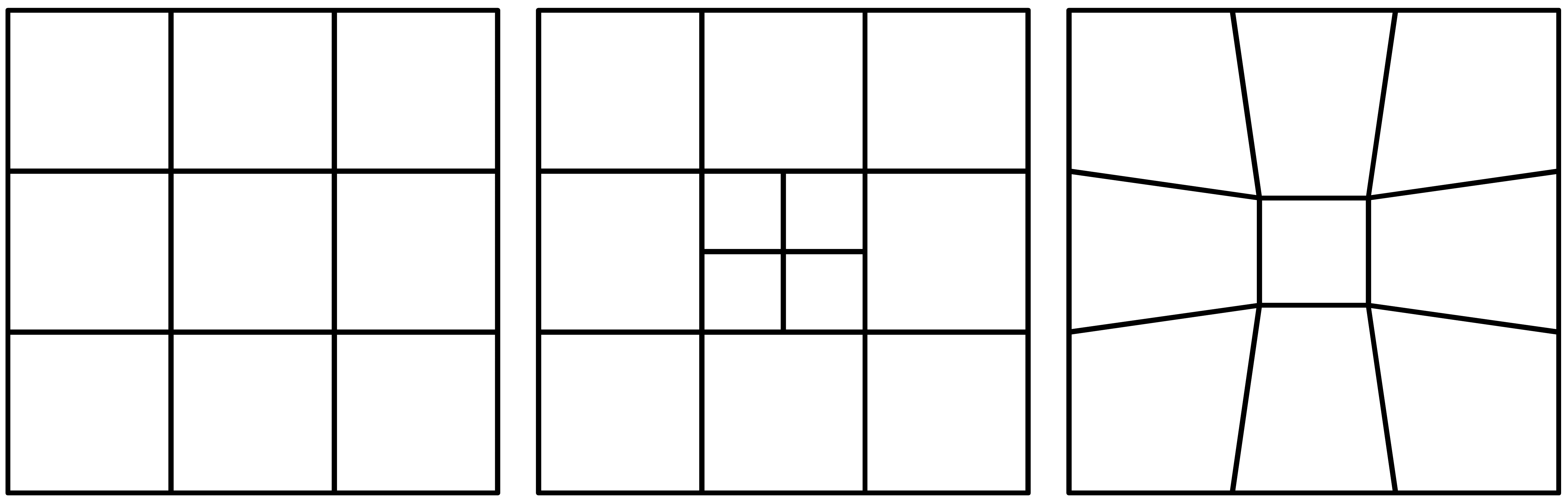
H-refinement relies on increasing the total number of grid elements (e.g., nodes or cells) within a base grid for which the original structure remains fixed. The technique, also known as mesh enrichment or local refinement, modifies the grid at regions tagged for increased resolution. Frequently, the method is carried out by subdividing grid elements into smaller self-similar components. In Figure 1, the example depicting h-refinement shows a single refinement level. A second level of refinement could involve subdividing the refined cells at the center of the domain into four even smaller cells. Generally, a maximum number of refinement levels allowed must be defined.
H-refinement can be realized by applying two distinct methodologies. One approach is to include added grid elements directly into the original base grid; all elements are solved on a single grid throughout the simulation. This method requires data storage procedures and solvers capable of handling unstructured grids. Alternatively, h-refinement can be achieved by considering the additional elements at increased resolution levels as distinct grids that are dynamically created or removed. In this manner, each refined grid can remain structured and be individually solved using algorithms developed exclusively for uniform or rectangular grids. Here, communication among different levels of refinement takes the form of boundary and initial conditions setting for the different grids.
R-refinement techniques, commonly referred to as mesh moving or global refinement, relocate mesh nodes to regions warranting increased resolution and subsequently increase grid element concentration at the areas with the greatest inaccuracies. However, the total number of grid points is maintained constant. Unlike h-refinement, r-refinement around a region is necessarily accompanied by coarsening at another. Figure 1 shows simple schematics of h-refinement and r-refinement at the center of a simple nine element quadrilateral grid.
Both adaptive gridding techniques have advantages and drawbacks associated with them. An advantageous distinguishing feature of r-refinement is smoother transitions in grid resolution. In contrast, h-refinement ordinarily operates on grids with abrupt discontinuities among the different refinement levels allowed. Acute disruptions in resolution are undesirable and may lead to interface problems. The constant number of grid elements maintained throughout a simulation using r-refinement could prove beneficial; a fixed number of elements simplifies solution algorithms and is helpful in parallel computing implementations. It could appear that the achievable improvement to solution accuracy with r-refinement is limited by the total number of grid elements or nodes, and that such a restraint is not inherent to h-refinement. However, it is important to note that the available computational resources, and not the number nodes, are the true limitation to accuracy. At the limit of computational capacity, both h- and r-refinement can only increase local refinement at the expense of coarsening elsewhere. More accurately, r-refinement's disadvantage lies in its need to determine global resolution (i.e., total number of grid elements) a priori. A poorly selected domain-wide number of elements will limit solution accuracy if too low and hinder efficiency if overly large. The requirement may be especially important when dealing with multiple and concurrent calls for increased resolution within different regions of a domain. This prerequisite is not essential to h-refinement. Additionally, h-refinement can guarantee a minimum solution accuracy level for all fields throughout the full domain by disallowing coarsening beyond a base grid resolution. R-refinement can be thought of as an optimization problem; the technique attempts to determine the best grid configuration possible under user-defined computational constraints. In h-refinement an optimal grid is not necessarily sought or possible. Typically, the discrete and bounded refinement levels used for adaptation with h-refinement schemes negate optimization. H-refinement is more frequently applied as a simple technique to identify regions that would likely benefit from increased resolution and readily refine at these locations if additional computational resources are available. The procedure may lead to an acceptable increase in solution accuracy by utilizing simpler adaptive algorithms that may be significantly less burdensome than those invoked by r-refinement methods. Neither refinement technique can be labeled as superior. While mesh movement seems better equipped to optimize resolution and computational workload, achieving an optimal grid may not be straightforward. Under such conditions the advantages of mesh enrichment could be of greater value.
3.1. Grid Structuring
Grid structures applied in numerical modeling may be categorized as structured or unstructured. The distinguishing feature between them refers to the data structure associated with each, rather than visual traits. Data on a structured grid can be arranged into a rectangular matrix; cells and nodes can be identified through integer indices (e.g., i, j, k). The requirement brings forth regular grid patterns and most often quadrilateral or hexahedral elements. Additionally, the data arrangement in structured grids reduces memory requirements compared to unstructured ones.
In contrast to structured grids, data from unstructured grids cannot be arranged by applying simple integer indexing and full connectivity must be defined and stored for each node. Unstructured grid cells are defined as a group of nodes that encompass an element of any geometry. These grids can be built using triangles, quadrilaterals, tetrahedra, hexahedra, or any polygon or polyhedron, including combinations of elements with different geometries. The irregularity of unstructured grids allows greater versatility in their assembly compared to structured grids. This flexibility in domain discretization has made unstructured meshes popular in simulations dealing with complex geometries and a common choice to model fluid mechanics [15].
Typically, finite-difference methods are used with structured grids and finite-element (or finite-volume) methods are used with unstructured grids. Both methods are well developed for the solution of hyperbolic partial differential equations of the type encountered in atmospheric models. Higher-order spatial approximations are available for both types of methods; therefore, the desired level of accuracy can be achieved with either. In general, higher-order methods in atmospheric models must be used together with flux-correction or filtering algorithms to avoid the generation of spurious oscillations that may lead to undesirable effects such as non-monotonic and unphysical (e.g., negative concentrations in air quality models) solutions or even instabilities. Using higher-order difference approximations or higher-order elements is known as p-refinement, an alternative to the adaptive grid h- or r-refinement techniques described above for increasing solution accuracy. The decision of using an explicit or an implicit scheme must made for time integration; it does not depend on the spatial grid and whether it is structured or unstructured. Hence, either option is available both with finite-difference and finite-element methods.
Mesh enrichment (i.e., h-refinement) can be implemented into both structured and unstructured grids. Often, refinement involves subdividing cells into equal self-similar elements; quadrilaterals and hexahedra are divided into four or eight smaller elements respectively. Likewise, techniques are available to systematically divide triangular and tetrahedral grid elements. For structured grids, mesh enrichment may decimate the regularity in grid elements and render original solution algorithms inapplicable, unless refinements are treated as distinct grids, like previously described for nested grid methods. H-refinement is more compatible with unstructured grids. Given the arbitrary arrangement of cells within an unstructured domain, initial solution algorithms will generally also be applicable to the refined grid.
Mesh movement (i.e., r-refinement) can also be achieved regardless of grid structure. The technique is clearly well suited to structured grids; despite node movement, the regularity and connectivity of grid elements remains intact. Nevertheless, solution algorithms designed for structured grids may have also been developed assuming uniformity and be invalid under a non-uniform grid. Solver incompatibility can be addressed by applying a coordinate transformation to the governing equations and grid, from non-uniform in physical space to uniform in computational space. The transformation must be applied each time the grid is restructured and may significantly increase the method's overhead. Mesh movement on unstructured grids can be simpler if the solution algorithms available are capable of handling irregular, non-uniform grids from the start.
3.2. Error Estimation
The objective of increasing solution accuracy through adaptive gridding can only be met if adaptation is driven by an efficient indicator of the solution error in a spatial field. The concept of error equidistribution has been used to describe the adaptive grid process; grids are reconfigured to result in an equal amount of error for all grid elements [16]. However, directly quantifying error is not a straightforward task. Quantitative analysis of resolution-induced error in advection algorithms has been previously investigated. For advection schemes, a Fourier method can estimate error (i.e., numerical diffusion) as a function of grid resolution [17]. The estimation becomes much more complex after integrating other physical and chemical processes into the system, particularly nonlinear transformations. Additionally, exact error quantification cannot be used as a refinement driver a priori, as the error itself depends on grid structure after adaptation.
Typically, adaptive grids use an error indicator in place of solution error to drive refinement. The error indicator may be a rudimentary calculation related to the error. For instance, estimates of the truncation or interpolation error may be applied. It is also common to rely on physical features that are known to efficiently signal locations where the error is most sensitive to grid resolution. In air quality modeling, for example, concentration gradients or curvatures can be used to trigger refinement and effectively increase solution accuracy. The selection of an error indicator to drive refinement is more critical to r-refinement than h-refinement. For mesh moving refinement, adaptation acts as an optimization processes by which error is minimized with a fixed amount of available resolution. Since refinement at one region necessitates coarsening at another, effective adaptation criteria truly representative of solution error are crucial. In mesh enrichment, base-level solution accuracy is generally guaranteed. Refinement augments resolution at selected locations and increases total grid resolution. An optimal grid configuration is not necessarily achieved nor pursued. Instead, mesh enrichment may simply allocate additional resolution in an attempt to sufficiently increase solution accuracy.
4. Antecedents of Adaptive Grid Air Quality Modeling
Research efforts investigating adaptive gridding in meteorological modeling precede those exploring the technique as an option for air quality simulation. The motivations and methodologies for adaptive grid refinement in both atmospheric realms are very much alike. The earliest attempt to simulate atmospheric flows using an adaptive grid was reported by Jones et al. [1]. In the model described, two levels of nested grids were allowed to move within a larger domain while tracking a tropical cyclone identified from the surface pressure field.
Subsequent applications of adaptive gridding in atmospheric modeling were described by Skamarock et al. [7,18]. In these simulations, grid refinement was based on the method of Berger and Oliger [19]. This approach to adaptive gridding achieves dynamic refinement by nesting rectangular subgrids of arbitrary orientation at regions necessitating enhanced resolution within a coarse-resolution base grid. Subgrids may overlap and multiple grid levels with increasing resolution can coexist. Estimates of truncation error at each grid point are used to flag the locations requiring improved resolution. Flagged points are clustered and rectangular subgrids encompassing each cluster are created. The procedure is performed at each level of resolution until no further refinement is required or a user-defined maximum level is reached.
An alternative strategy to adaptive gridding in meteorological modeling was reported by Dietachmayer and Droegemeier [20,21]. This method utilizes r-refinement driven by a weight function calculated from the spatial fields of selected physical properties, typically based on gradients and curvatures. Similar to other r-refinement algorithms, a coordinate transformation from irregular physical space to uniform computational space is applied to the governing system of equations.
5. Adaptive Grids in Air Quality Models
Application of adaptive grids in air quality modeling has been explored for over 10 years. Three distinct efforts to implement adaptive gridding techniques into Eulerian air pollution models can be identified. These undertakings can each be traced back to Tomlin et al. [22], Srivastava et al. [23], and Constantinescu et al. [24]. The techniques presented by Tomlin et al. [22] and Srivastava et al. [23] have undergone substantial development thereafter, and evolved from simple exercises designed to prove the worthiness of adaptive gridding in air pollution modeling to elements of regional air quality models applied to realistic simulations. The aforementioned approaches to adaptive grid modeling are vastly different; methods applied to achieve improved results are unique to each. However, the goal and many of the conclusions reached from analysis of modeled results are common to all. In this section we describe the main characteristics of each of these adaptive grid modeling techniques, as well as common challenges encountered and shared conclusions. A summary of the methods' characteristics is also presented in Table 1.
5.1. Reported Adaptive Grid Methods in Air Quality Modeling
An adaptive grid method applicable to air pollution modeling using unstructured grids is described by Tomlin et al. [22]. The method is applied to an unstructured triangular grid model which solves the discretized atmospheric diffusion equation using a finite-volume approach. Grid refinement is achieved through mesh enrichment (i.e., h-refinement). Original grid nodes remain fixed and refinement is accomplished by splitting each triangle into 4 smaller, similar triangles. The process can be extended to any user-determined level of refinement and derefinement simply involves merging elements contained within the same parent triangle. The refinement technique is illustrated in Figure 2. Adaptation is driven by the spatial error estimated as the difference between solutions calculated using first- and second-order methods. A test case simulated dispersion of a concentrated NOx plume within background atmospheres with varying degrees of pollution. The NO concentration field was selected to estimate spatial error and drive refinement limited to a maximum of two levels. In the simulation, refinement winds up concentrated around pronounced spatial gradients. The adaptive grid captures features in the ozone and NO2 concentration structures unseen in a simulation without refinement, near the point source and further downwind. Additionally, a significant difference in total NO2 mass is observed between adapted and unadapted simulations. The authors attribute the discrepancy to nonlinear chemistry, which renders ozone and NOx concentrations grid resolution dependent.
The adaptive gridding method of Tomlin et al. [22] has been subsequently applied to model the dispersion of nuclear contamination [26] and air pollution formation across central Europe [27]. These simulations extended into the regional scale and incorporated vertical layering and mixing, space-and-time-varying three-dimensional meteorological fields, dry deposition, and pollutant transformations (e.g., nuclear decay or chemical reactivity). In these studies, concentrations estimated using adaptive grids exhibited closer agreement to concentrations calculated under fine resolution than those attainable using coarse grids or nested grids placed over main pollutant sources. Furthermore, adaptive grids required only a fraction of the computer time necessary for the fine resolution simulations. Implementation of adaptive gridding along the vertical domain has also been reported [25,28]. The three-dimensional adaptive grid method uses an unstructured tetrahedral grid. Refinement is based on the same strategy previously described for the horizontal adaptation and is achieved by subdividing tetrahedral elements into 6 to 14 smaller tetrahedra depending on cell location and the number of edges tagged for refinement. In one test case, the adaptive grid method was used to model an elevated NO point source under conditions representative of different stability classes [28]. Adaptation was driven by node-to-node concentration gradients. The results demonstrate the significance of vertical resolution in estimating accurate pollutant concentrations. This is especially true downwind of sources and under neutral-to-stable atmospheric conditions, which frequently lead to limited mixing and large gradients at inversion layers.
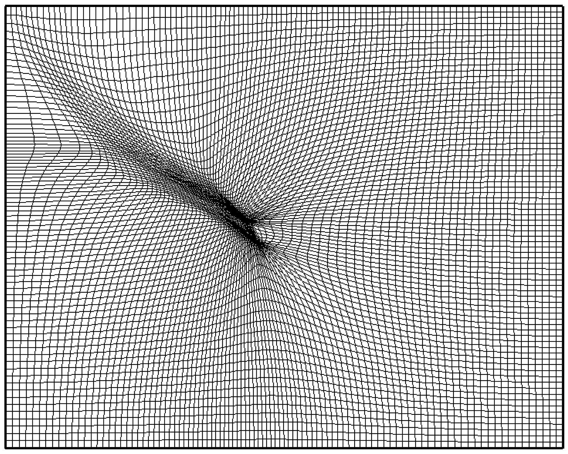
The use of mesh movement (r-refinement) as an adaptive grid strategy in air quality modeling was first reported by Srivastava et al. [23]. The proposed adaptive grid algorithm maintains the number of grid cells fixed throughout the simulation and operates on a structured grid. Nodes are allowed to relocate across the domain in an attempt to minimize solution error. However, grid topology remains unaltered. Use of non-uniform grid elements requires that a transformation from Cartesian to curvilinear coordinates be applied to governing equations and node positions. This transforms the grid from non-uniform in physical space to uniform in computational space, and allows the finite-volume solution procedures designed for a physically uniform grid to be applied to a non-uniform dynamic grid. Adaptation (i.e., grid movement) is controlled by a weight function based on an error estimate defined as the difference between the values at each cell and those obtained by interpolation of values in neighboring cells. A combination of species' concentrations may be selected as values used in the weight estimation. Weights are normalized, smoothed, and integrate several parameters that can be used to control the degree of adaptation. During adaptation, grid nodes are relocated and clustered around areas bearing large weights. After the grid is modified, it is necessary to reorganize solution fields onto the new grid applying a redistribution procedure. The newly generated solution fields can then be used to recalculate spatial error (i.e., weights) in an iterative procedure that continues until a grid convergence criterion, defined as a maximum node movement relative to initial grid spacing, is met.
Several tests were performed using this adaptive grid algorithm to evaluate its performance including simulations of rotating conical concentration distributions [23], a reacting pollutant puff [23,29], and dispersion of a power plant plume [30]. The simulation of single and multiple rotating conical distributions confirmed a significant increase in solution accuracy compared to static grid simulations and demonstrated the adaptive grid's ability to better resolve features involving steep gradients or discontinuities. An important observation is mentioned by the authors; while the adaptive grid provides an improvement over fixed grids, the solution accuracy may still be limited by the total number of grid nodes in the simulation. A closer approximation to the exact solution may require that the number of grid nodes (i.e., cells) be increased, especially if multiple features simultaneously require increased resolution to be well resolved. The results from tests that modeled a reactive pollutant puff demonstrated that the adaptive grid algorithm better simulates nonlinear chemical transformations of pollutant distributions compared to static grid models. Srivastava et al. [30], modeled a plume from an elevated point source resembling a power plant stack with a simplified chemical mechanism using adaptive and static grids. The authors find that the adaptive grid method decreases plume dispersion and has a significant effect on modeled ozone concentrations. The adaptive simulation was able to capture the small scale ozone plume structure near the source as well as high ozone concentrations at large distances downwind. These features are not observed when using a static grid. The test further demonstrates that the transport and nonlinear chemical processes relevant to an ozone plume's “early”, “intermediate”, and “mature” stages can only be adequately modeled by adaptive gridding or drastically increasing the number of cells in a much more computationally expensive simulation.
To demonstrate the computational expense and accuracy gained, CPU times with static and adaptive grids were compared for the reactive pollutants puff test [23]. The solution with an adaptive grid took 9 times longer than the solution on a static grid with the same number of grid cells. However, the accuracy of the adaptive grid solution was far superior as the minimum grid cell size around the puffs was 30–40 times smaller than the static grid cell size. The CPU time of a refined static grid solution using 9 times more cells was also measured. Note that this solution falls short of providing the minimum cell size and the accuracy achieved by the adaptive grid solution, yet its CPU time was 63 times longer than the adaptive grid's. These comparisons show that adaptive grids have the potential to offer accurate solutions at significant cost savings.
Implementation of r-refinement into a comprehensive regional chemical-transport model was first reported by Odman et al. [31]. Later, Garcia-Menendez et al. [32] developed an adaptive grid version of the Community Multiscale Air Quality modeling system (CMAQ) [33] using the adaptive grid algorithm proposed by Srivastava et al. [23]. CMAQ integrates advection, diffusion, deposition, gas-phase chemistry, aqueous-phase reactions, aerosol dynamics, and cloud processes into air quality modeling. The adaptive grid version of CMAQ (AG-CMAQ) performs a transformation of the original governing equations in curvilinear coordinates, which allows the existing numerical schemes to be applied on a non-uniform grid. Two-dimensional grid refinement is driven by a weight function estimated from a numerical approximation of the curvature in selected model variables. The weight function can incorporate concentrations of different species or alternative atmospheric variables and adjust the relative importance of each.
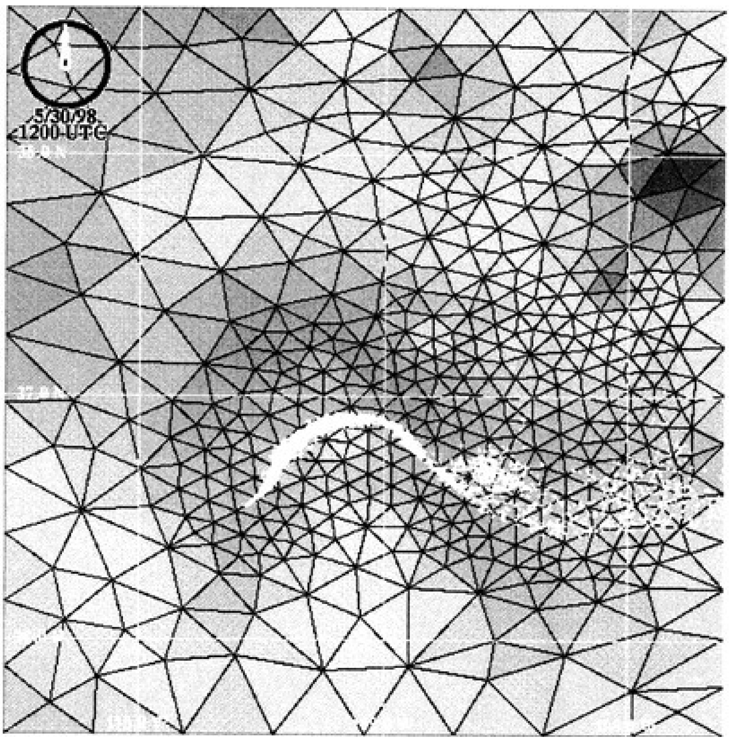
AG-CMAQ performance was evaluated by applying the model to simulate the air pollution impacts from an actual biomass burning event affecting air quality over a large urban area. Figure 3 illustrates the application. The focus was placed on fine particulate matter. This differs from most adaptive grid plume simulations previously reported, centered on ozone photochemistry. Additionally, results were compared to measurements at air quality monitoring sites, an assessment approach that had only been previously reported for adaptive grids by Lagzi et al. [27]. Three-dimensional meteorological and emissions data were prepared by a numerical weather prediction model and emissions processors. The evaluation showed that AG-CMAQ reduced diffusion and produced better refined plumes compared to fixed grid CMAQ results. The mean fractional error relative to measurements was also reduced when using AG-CMAQ. Furthermore, the developers believe that AG-CMAQ may provide insight into atmospheric processes beyond that which can be gained from fixed grid CMAQ simulations.
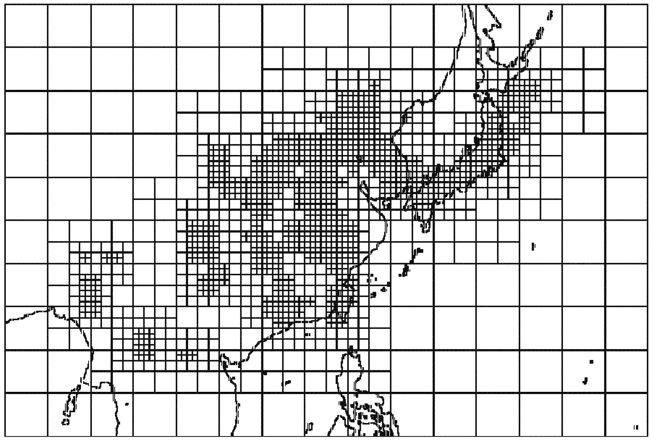
The adaptive grid method described by Constantinescu et al. [24] has also been implemented into a comprehensive chemical and transport model. The authors developed a mesh enrichment (i.e., h-refinement) technique based on a structured quadrilateral grid and limited to the horizontal plane. The technique is illustrated in Figure 4. In this method, coarse level cells are grouped into equilateral blocks, each containing an equal number of cells. Refinement is achieved by subdividing a block into smaller blocks. Each refined block maintains the same structure and number of cells as the original block from which they were derived. Refinement can continue up to a specified maximum level; smaller cells are produced and the total number of cells across the domain is increased. Derefining involves merging several blocks into a single coarser-level block. The block structure and number of cells enclosed within each block, remain constant throughout the simulation. Adaptation is driven by the curvature in horizontal concentration fields. The normalized root mean square concentration curvature is estimated for each block, and the maximum estimate among all vertical layers is compared to user-defined tolerances to indicate refinement or derefinement. Simplified tests simulating atmospheric dispersion indicated that the adaptive grid is capable of producing more accurate results than coarse and nested grids.
The adaptive grid methodology of Constantinescu et al. [24] was integrated into the Sulfur Transport and dEposition Model (STEM) [34]. STEM includes three-dimensional representations of dispersion, deposition, chemical transformation, and cloud processes. An adaptive grid simulation focused on ozone formation over East Asia during one week was carried out using four levels of refinement. Over 100 chemical species and 200 chemical reactions are considered in the model. Yearly averaged emissions inventories and prognostic weather simulation results were included as inputs. Different species were used to estimate concentration curvature and drive adaptation. The curvature in ozone proved least useful, while curvature estimates accounting for ozone precursors (NO, NO2, and HCHO) produced better results. An increase in accuracy was observed when applying an adaptive grid relative to coarse resolution results. Two interesting observations are also discussed: (1) the increase in solution accuracy is highly dependent on the user defined refinement tolerances, and (2) the total number of grid cells decreases with time until becoming fairly stable. Special attention was given to implementation of the adaptive grid method into parallel computing systems, facilitated by the domain's division into self-similar blocks. A computational cost is acknowledged for adaptive gridding. However, the computational requirements were significantly lower than those necessary for simulations performed at the finest grid resolution allowed in the adaptive grid application. For the application described, wall-clock times of STEM runs with static and adaptive grids were compared. An adaptive grid run of comparable accuracy required only a quarter of the time spent in a static fine grid run.
5.2. Common Challenges
The methodologies described in Section 4.1 follow different approaches to adaptive grid integration into air pollution modeling. However, all attempts have encountered common challenges. These common obstacles and the strategies applied to overcome them merit attention and are discussed in this subsection.
5.2.1. Refinement Criterion
We have previously mentioned that an essential component of any grid refinement technique is an error estimation that serves as a refinement criterion. All applications of adaptive gridding to air quality modeling previously reported have relied on atmospheric concentration spatial fields. An error estimate calculated from the difference in first-order and second-order approximations of local concentrations was described in Tomlin et al. [22]. A simpler error calculation based on the gradient between neighboring concentration values was applied in Ghorai et al. [28]. A numerical approximation of the curvature of concentration fields was introduced by Srivastava et al. [23] and has been used in later studies [24,32]. The different error estimations have all proven adequate. For simulations analyzing secondary pollutant fields, results indicate that spatial error calculations that consider precursor species outperform those that focus solely on the secondary pollutant.
5.2.2. Refinement Control
A need to constrain refinement intensity has also been identified in all previous investigations. Uncontrolled adaptation may lead to excessive refinement. Control parameters are implemented into the refinement criteria estimates previously described to normalize and smooth spatial error calculations. Mesh enrichment methods additionally require that user-defined upper and lower tolerances be set to trigger adaptation, directly controlling the degree to which grids are reconfigured. Furthermore, mesh enrichment techniques constrain adaptation to a maximum number of refinement levels. In the iterative mesh moving method previously described, a maximum number of relocation operations and minimum node movement relative to initial grid spacing are defined to stop adaptation.
Some concern about abrupt transitions in grid resolution has been expressed in past adaptive gridding exercises. The existence of neighboring grid elements refined to very different degrees may lead to errors and the loss of features resolved under the fine resolution if advection transports the features into coarse resolution regions prior to adaptation. A safety layer encompassing high resolution regions is proposed as a solution by Tomlin et al. [25]. The problem has also been addressed by significantly smoothing the error estimation driving adaptation [23]. In r-refinement no boundaries between different resolution levels are created and smoothing can guarantee changes in grid size are gradual. Special care must be given to refinement along domain borders, as boundary conditions are generally only available at coarser resolution. Domain design should consider maintaining features that will call forth considerable refinement distanced from the domain edges. The moving mesh algorithm developed by Srivastava et al. [23] only allows node movement along the lateral domain boundaries, limiting the refinement attainable along these edges. The same strategy is applied in AG-CMAQ. In the adaptive grid model developed by Constantinescu et al. [24] the cell blocks along lateral domain boundaries are maintained at the coarsest level throughout the simulation, and each subsequent cell block is only allowed to adapt to one additional refinement level.
5.2.3. Adaptation Frequency
As adaptability is integrated into more complex atmospheric systems, the grid refinement process may become increasingly taxing, especially when applied to comprehensive chemical-transport models. Therefore, it may be necessary or desirable to apply grid adaptation at intervals greater than solution frequency. Ghorai et al. [28] found that performing grid adaptation every 20 min is sufficient to produce accurate results and reduces the computational requirements of a three-dimensional elevated plume simulation. A 5 min adaptation interval is used in the regional air quality case presented in Lagzi et al. [27]. In their simulation of air quality over East Asia, Constantinescu et al. [24] tested adaptation intervals from 1 to 6 h and determined that 3 hours provided an adequate balance between solution accuracy and computational cost. The reactive plume simulation of Srivastava et al. [30] applies grid adaptation at a frequency equivalent to every 4 solution time steps. The adaptive grid version of CMAQ developed by Garcia-Menendez et al. [32], carries out adaptation once every output time step, set to 15 min in the application described. A related concern is the existing lag between adaptation and solution; error calculations that drive adaptation are estimated using the solution at the end of a time step, but the grid generated is applied towards solution of the following time step. To address this issue, quadratic interpolants have been used to predict the evolution of spatial error at a future time step and determine refinement [22]. Such an approach may become increasingly useful as adaptability is implemented into more complex models and the frequency of adaptation must be reduced.
5.2.4. Preadaptation
Preadaptation has also been identified as a process that might be important in effective grid refinement. The strategy is of particular relevance to point sources which might immediately dilute into coarse cells and lose plume features prior to any adaptation. The plume simulation carried out by Tomlin et al. [25] addressed the issue by placing the modeled stack within a subdomain and using the subdomain concentration as an internal boundary condition, an approach similar to grid nesting. Subsequent applications of this adaptive grid method have commenced from grids initially refined around major pollutant sources (e.g., point sources [28], cities [26,27]). A grid preadaptation step was proposed by Srivastava et al. [23]. Under this procedure, a grid is adapted from the initial concentration field using the same error weight function estimation applied throughout the simulation. For sources that begin to emit at the start of the simulation, emissions are assumed to occur prior to initiating the run. Although preadaptation was not considered in the simulations discussed in Constantinescu et al. [24], the authors acknowledge that a transient phase characterized by heavier refinement and observed during the initial stages of all runs might be attributable to coarse resolution around major sources at the onset.
5.2.5. Interpolation
Interpolation of coarse or uniformly distributed data onto adapted grids is an important component of all adaptive air quality modeling methods reported. The operation is essential during three processes of an adaptive grid air quality model: emissions, meteorology, and solution redistribution. The procedure for processing emissions must be applied after each grid adaptation operation. Different interpolation schemes have been used to interpolate area sources onto adapted non-uniform grids. Additionally, point sources must be relocated to appropriate cells after grid reconfiguration. Emissions processing can become taxing, especially for mesh moving methods that use cells with irregular geometries [32]. Meteorological inputs, whether from numerical weather prediction models or synoptic observations, are typically uniformly spaced and provided at a resolution coarser than that of refined grids. Ideally, meteorological inputs should be provided on the same adaptive grids. A system with adaptive grid capability that attempts to couple simple air pollutant dispersion models with meteorology models was reported by Bacon et al. [35] and is further described in Section 6. Mapping of meteorological fields onto required locations on an adapted grid is necessary and can be achieved through interpolation techniques. Nonetheless, the interpolation should ensure conservation and produce minimally modified fields [25]. The most recurrent interpolation operation in an adaptive grid algorithm is redistribution of solution fields onto modified grids after applying adaptation. Here, conservation is paramount. With grid enrichment methods, the operation may be as simple as linear interpolation [24]. More elaborate interpolation techniques have been applied to solution interpolation onto unstructured triangular and tetrahedral based grids, including a conservative rezoning algorithm and cell-vertex method [25]. Under mesh moving techniques, the movement of nodes over solution fields can be considered as equivalent to advective fluxes crossing cell boundaries. Solution redistribution procedures using a conservative interpolation equation or monotonic advection scheme have been previously described [23,32]. It is likely that a significant fraction of the computational cost associated with adaptive grid air quality modeling is attributable to solution redistribution operations. This is especially true for iterative procedures. The overhead from adaptation must be kept in check by defining appropriate adaptation intervals and refinement parameters. Finding an adequate balance between adaptation efficiency and computational workload is important to achieve an effective operational model.
5.2.6. Time-Stepping
One characteristic of adaptive grid air quality models that can severely hinder performance is excessively small process time steps applied uniformly throughout the domain. It is common practice in air pollution models to apply the domain-minimum time step, typically fixed by the characteristic time for advection, at every point [24,28]. Therefore, the domain-wide solution time step is determined by the grid cells subjected to the highest resolution and greatest wind speeds. This guarantees that the Courant stability condition is met. However, as grids are refined solution time steps become increasingly small. Applying the minimum solution time step across the entire grid regardless of the individual needs at each location is an inefficiency typically encountered in air quality models that may render adaptive gridding prohibitive. This concern is especially relevant when applying adaptive grid algorithms to comprehensive air quality models. The problem can be controlled by constraining the degree of refinement allowed as previously described. Alternatively, a variable time step algorithm was implemented into the adaptive grid version of CMAQ to address the issue [32]. Under this technique, a local solution time step is assigned to each grid cell and the computational cost associated with adaptive gridding can be notably reduced. The local time steps are all integer divisors of a synchronization time step used to advance in time a synchronized global solution [36].
5.2.7. Subgrid Scale Parameterizations
Finally, an especially significant concern about adaptive grid air quality modeling is the applicability of subgrid parameterizations to grids with non-uniform resolution and highly refined regions. The issue has not yet been addressed in reported research efforts. Parameterizations for physical processes (e.g., turbulence, cloud processes) must be valid for the refined grid. The dependence of these parameterizations on grid resolution may bring into question their validity across the entire domain if considerable differences in grid resolution are allowed. Furthermore, if resolution is sufficiently increased, some parameterizations might not be required and their inclusion could adversely affect solution accuracy. The concern is also relevant to adaptive grid modeling in other atmospheric realms. For instance, one adaptive grid weather prediction model assigns an adjustment factor, determined by cell area, to each cell and uses this factor to regulate the degree to which the convective parameterization is applied at individual cells [35]. Similarly, techniques that integrate dependence on grid resolution into the parameterizations of adaptive grid air quality models may have to be considered.
6. Additional Applications of Adaptive Grid Modeling in Atmospheric Sciences
As adaptive grid modeling is being explored in air quality modeling, concurrent efforts to integrate the technique into weather prediction and global circulation models have been reported. Attempts to apply adaptive grids in comprehensive meteorological models have been limited with few recent developments. A noteworthy application is the Operational Multiscale Environmental model with Grid Adaptivity (OMEGA) [35]. This numerical weather prediction model operates on a three-dimensional unstructured grid constructed from triangular prisms. Adaptation is carried out by adding or removing vertices at the centroids of cells tagged for refinement, subdividing cells, and restructuring node connections to minimize aspect ratio. An interesting feature of the model is the addition of dispersion modeling. Three distinct atmospheric dispersion techniques are integrated into OMEGA: Eulerian, Lagrangian particle, and probabilistic puff modeling. The techniques simplify pollutant transport by relying on averaged wind fields, parameterizing turbulent diffusion, and neglecting chemical transformation processes. Although these methodologies are not new, their incorporation into an adaptive grid meteorological model is of interest. With their inclusion, OMEGA allows embedded dispersion models to operate under high resolution meteorological fields. Furthermore, adaptation of the meteorological model can be driven by the pollutant plume itself [35]. Figure 5 illustrates grid adaptation to a plume in OMEGA. In this manner, a coupled meteorological-air-quality model that continuously exchanges data to drive the adaptation is established.
Much of the progress recently reported pertaining to adaptive grid modeling in atmospheric science involves incorporation of the technique into general circulation models. The motivation to integrate adaptive gridding into global models is largely analogous to that driving incorporation into air quality and weather models: models simulate atmospheric processes covering a wide range of scales and available computational resources are unable to explicitly resolve all processes involved. Therefore, it is not surprising to find that adaptive gridding techniques explored in climate models are frequently equivalent to those applied to air pollution modeling. However, the spatial and temporal scales of interest are very different to those in air quality simulations. In addition, the spherical nature of the global modeling domain and differences in simulated processes result in very different grid refinement requirements.
Nonetheless, future applications of adaptive gridding in air quality modeling may benefit from previous and ongoing efforts to integrate the technique into global models. Hubbard and Nikiforakis [37] applied the grid refinement technique of Berger and Oliger [19] previously explored in regional weather modeling, to global atmospheric modeling. Adaptive grid climate modeling on unstructured triangular or tetrahedral based grids has been explored by Behrens et al. [38–41]. Here, adaptation is achieved by bisecting triangular or tetrahedral elements. Jablonowski et al. [42–44] explored block-structured adaptive gridding within a global atmospheric model. The grid refinement technique implemented in these applications is similar to that applied to air quality modeling by Constantinescu et al. [24] and is illustrated in Figure 6. Refinement is achieved by organizing the domain into a block structured two-dimensional grid and further dividing blocks tagged for refinement into smaller self-similar units containing a fixed number of cells. Adaptation is allowed to proceed for several levels and each block is solved independently. A refinement technique applicable to three-dimensional grids based on any geometric element was described by Weller and Weller [45]. The method has been explored on reduced latitude-longitude and hexagonal icosahedral grids [45], cubed sphere and triangular icosahedral grids [46], and polygon based grids [47]. Moreover, an interesting approach to adaptation was presented by Weller [47] where future refinement requirements are predicted at each adaptation step, allowing less frequent grid restructuring and diminished costs associated with restructuring the grid. Predictions are attained by advancing the solution by one adaptation time step on a coarse grid and estimating refinement criteria from this solution to generate a refined grid effective for the entire adaptation step. Additional research efforts exploring atmospheric modeling with unstructured Voronoi tessellations and C-grid discretization have been recently reported [48,49]. These grid generation techniques provide a natural framework for multiscale modeling and could effortlessly incorporate adaptive gridding in the future.
7. Concluding Remarks
Adaptive grid methods have not been fully explored in atmospheric modeling. Early attempts in weather prediction did not flourish and this field remained dominated by static nested grid methods. There have been a few recent attempts to integrate adaptive grids into air quality modeling but once again these attempts did not enjoy wide acceptance. Future undertakings should consider several key factors if greater interest in the technique is sought. The prevalence of community-driven models in atmospheric sciences today makes compatibility with existing model frameworks an indispensible requirement for increased use of adaptive gridding methodologies. Additional applications that go beyond typical power plant plume and ozone chemistry simulations are necessary to further demonstrate the worth of dynamic grid refinement. Finally, adaptive grid air quality models will have to be accompanied by equivalent increases to the resolution of emissions and meteorological inputs to truly reach their full potential.
What looks promising for adaptive grids is the presence of a vibrant support by the global climate community who acknowledge reaching a plateau after years of improvement in accuracy, mainly driven by progress in high performance computing. Adaptive grid methods are viewed as a means to reignite model advancement and a long term solution for dealing with the multiscale nature of the climate system [50]. Workshops are being organized to discuss the potential of adaptive grid methods in global scale modeling [51]. The range of scales covered by climate models is vast. For this reason, adaptive gridding might prove most crucial to future climate modeling. The recent appearance of numerous papers on adaptive grid use in global models may be the early sign of an explosive growth in this field.
The potential returns of adaptive grids are enormous while the risks are relatively small. The methods have matured through advancements in computational fluid dynamics and wide use, for example, in aerospace engineering applications. The difficulties will be faced in developing parameterizations for processes that cannot be resolved by adaptive gridding. In our view, the problem will eventually die out as adaptive grids continue to provide increased grid resolution. Nonetheless, the issue must be dealt with in the interim. The wide range of scales provided by adaptive grids will necessitate resolution dependent parameterizations and this may appear as a daunting task. However, what is faced today by increasing grid resolution uniformly or through grid nesting is the exact same problem: parameterizations that made sense for coarse grid resolution must be rethought as grid resolution increases. We must simply develop a culture of designing resolution dependent parameterizations upfront instead of revising the parameterizations every time model resolutions change. For these reasons, we believe that the time is right to invest in the development of adaptive grid models.


| Original Publication | Grid Structure | Refinement method | Refinement criteria applied | Implementation into operational air quality model | Vertical adaptivity |
|---|---|---|---|---|---|
| Tomlin et al. [22] | Unstructured triangular or tetrahedral | Single grid h-refinement | 1st and 2nd order solution difference; concentration gradient | Eulerian grid model | Yes |
| Srivastava et al. [23] | Structured quadrilateral | R-refinement | Interpolation error; concentration curvature | CMAQ | No |
| Constantinescu et al. [24] | Uniform quadrilateral with nested refinements | Multigrid h-refinement | Concentration curvature | STEM | No |
Acknowledgments
This research was supported in part by the U.S. Department of Defense, through the Strategic Environmental Research and Development Program (SERDP) under SERDP project number RC-1647 and by the U.S. Department of Agriculture Forest Service through the Joint Fire Science Program (JFSP) under JFSP project number 08-1-6-04.
References
- Jones, R.W. A nested grid for a 3-dimensional model of a tropical cyclone. J. Atmos. Sci. 1977, 34, 1528–1553. [Google Scholar]
- Miyakoda, K.; Rosati, A. One-way nested grid models: The interface conditions and the numerical accuracy. Mon. Weather Rev. 1977, 105, 1092–1107. [Google Scholar]
- Phillips, N.A.; Shukla, J. On the strategy of combining coarse and fine grid meshes in numerical weather prediction. J. Appl. Meteorol. 1973, 12, 763–770. [Google Scholar]
- Clark, T.L.; Farley, R.D. Severe downslope windstorm calculations in two and three spatial dimensions using anelastic interactive grid nesting: A possible mechanism for gustiness. J. Atmos. Sci. 1984, 41, 329–350. [Google Scholar]
- Zhang, D.-L.; Chang, H.-R.; Seaman, N.L.; Warner, T.T.; Fritsch, J.M. A two-way interactive nesting procedure with variable terrain resolution. Mon. Weather Rev. 1986, 114, 1330–1339. [Google Scholar]
- Pleim, J.E.; Chang, J.S.; Zhang, K.S. A nested grid mesoscale atmospheric chemistry model. J. Geophys. Res. Atmos. 1991, 96, 3065–3084. [Google Scholar]
- Skamarock, W.C.; Klemp, J.B. Adaptive grid refinement for 2-dimensional and 3-dimensional nonhydrostatic atmospheric flow. Mon. Weather Rev. 1993, 121, 788–804. [Google Scholar]
- Debreu, L.; Blayo, E. Two-way embedding algorithms: A review. Ocean Dyn. 2008, 58, 415–428. [Google Scholar]
- Alapaty, K.; Mathur, R.; Odman, T. Intercomparison of spatial interpolation schemes for use in nested grid models. Mon. Weather Rev. 1998, 126, 243–249. [Google Scholar]
- Smolarkiewicz, P.K.; Grell, G.A. A class f monotone interpolation schemes. J. Comput. Phys. 1992, 101, 431–440. [Google Scholar]
- Bott, A. A positive definite advection scheme obtained by nonlinear renormalization of the advective fluxes. Mon. Weather Rev. 1989, 117, 1006–1015. [Google Scholar]
- Colella, P.; Woodward, P.R. The piecewise parabolic method (PPM) for gas-dynamical simulations. J. Comput. Phys. 1984, 54, 174–201. [Google Scholar]
- Harris, L.M.; Durran, D.R. An idealized comparison of one-way and two-way grid nesting. Mon. Weather Rev. 2010, 138, 2174–2187. [Google Scholar]
- Odman, M.T.; Russell, A.G. On local finite-element refinements in multiscale air-quality modeling. Environ. Softw. 1994, 9, 61–66. [Google Scholar]
- Morgan, K.; Peraire, J. Unstructured grid finite-element methods for fluid mechanics. Rep. Prog. Phys. 1998, 61, 569–638. [Google Scholar]
- Baker, T.J. Mesh adaptation strategies for problems in fluid dynamics. Finite Elem. Anal. Des. 1997, 25, 243–273. [Google Scholar]
- Odman, M.T. A quantitative analysis of numerical diffusion introduced by advection algorithms in air quality models. Atmos. Environ. 1997, 31, 1933–1940. [Google Scholar]
- Skamarock, W.; Oliger, J.; Street, R.L. Adaptive grid refinement for numerical weather prediction. J. Comput. Phys. 1989, 80, 27–60. [Google Scholar]
- Berger, M.J.; Oliger, J. Adaptive mesh refinement for hyperbolic partial-differential equations. J. Comput. Phys. 1984, 53, 484–512. [Google Scholar]
- Dietachmayer, G.S.; Droegemeier, K.K. Application of continuous dynamic grid adaption techniques to meteorological modeling: Part I: Basic formulation and accuracy. Mon. Weather Rev. 1992, 120, 1675–1706. [Google Scholar]
- Dietachmayer, G.S. Application of continuous dynamic grid adaption techniques to meteorological modeling. Part II: Efficiency. Mon. Weather Rev. 1992, 120, 1707–1722. [Google Scholar]
- Tomlin, A.; Berzins, M.; Ware, J.; Smith, J.; Pilling, M.J. On the use of adaptive gridding methods for modelling chemical transport from multi-scale sources. Atmos. Environ. 1997, 31, 2945–2959. [Google Scholar]
- Srivastava, R.K.; McRae, D.S.; Odman, M.T. An adaptive grid algorithm for air-quality modeling. J. Comput. Phys. 2000, 165, 437–472. [Google Scholar]
- Constantinescu, E.M.; Sandu, A.; Carmichael, G.R. Modeling atmospheric chemistry and transport with dynamic adaptive resolution. Comput. Geosci. 2008, 12, 133–151. [Google Scholar]
- Tomlin, A.S.; Ghorai, S.; Hart, G.; Berzins, M. 3-D Multi-scale air pollution modelling using adaptive unstructured meshes. Environ. Model. Softw. 2000, 15, 681–692. [Google Scholar]
- Lagzi, I.; Karman, D.; Turanyi, T.; Tomlin, A.S.; Haszpra, L. Simulation of the dispersion of nuclear contamination using an adaptive Eulerian grid model. J. Environ. Radioact. 2004, 75, 59–82. [Google Scholar]
- Lagzi, I.; Turanyi, T.; Tomlin, A.S.; Haszpra, L. Modelling photochemical air pollutant formation in Hungary using an adaptive grid technique. Int. J. Environ. Pollut. 2009, 36, 44–58. [Google Scholar]
- Ghorai, S.; Tomlin, A.S.; Berzins, M. Resolution of pollutant concentrations in the boundary layer using a fully 3D adaptive gridding technique. Atmos. Environ. 2000, 34, 2851–2863. [Google Scholar]
- Srivastava, R.K.; McRae, D.S.; Odman, M.T. Simulation of a reacting pollutant puff using an adaptive grid algorithm. J. Geophys. Res. Atmos. 2001, 106, 24245–24257. [Google Scholar]
- Srivastava, R.K.; McRae, D.S.; Odman, M.T. Simulation of dispersion of a power plant plume using an adaptive grid algorithm. Atmos. Environ. 2001, 35, 4801–4818. [Google Scholar]
- Odman, M.T.; Khan, M.N.; Srivastava, R.K.; McRae, D.S. Initial Application of the Adaptive grid Air Pollution Model. In Air Pollution Modeling and Its Application XV; Borrego, C., Schayes, G., Eds.; Kluwer Academic/Plenum Publishers: New York, NY, USA, 2002; pp. 319–328. [Google Scholar]
- Garcia-Menendez, F.; Yano, A.; Hu, Y.; Odman, M.T. An adaptive grid version of CMAQ for improving the resolution of plumes. Atmos. Pollut. Res. 2010, 1, 239–249. [Google Scholar]
- Byun, D.; Schere, K.L. Review of the governing equations, computational algorithms, and other components of the models-3 Community Multiscale Air Quality (CMAQ) modeling system. Appl. Mech. Rev. 2006, 59, 51–77. [Google Scholar]
- Carmichael, G.R.; Peters, L.K.; Saylor, R.D. The STEM-II regional scale acid desposition and photochemical oxidant model. 1. An overview of moel development and applications. Atmos. Environ. Part A 1991, 25, 2077–2090. [Google Scholar]
- Bacon, D.P.; Ahmad, N.N.; Boybeyi, Z.; Dunn, T.J.; Hall, M.S.; Lee, P.C.S.; Sarma, R.A.; Turner, M.D.; Waight, K.T.; Young, S.H.; et al. A dynamically adapting weather and dispersion model: The Operational Multiscale Environment Model with Grid Adaptivity (OMEGA). Mon. Weather Rev. 2000, 128, 2044–2076. [Google Scholar]
- Hu, Y.; Odman, M.T. A variable time-step algorithm for air quality models. Atmos. Pollut. Res. 2010, 1, 229–238. [Google Scholar]
- Hubbard, M.E.; Nikiforakis, N. A three-dimensional, adaptive, Godunov-type model for global atmospheric flows. Mon. Weather Rev. 2003, 131, 1848–1864. [Google Scholar]
- Behrens, J. Adaptive atmospheric modeling: Scientific computing at its best. Comput. Sci. Eng. 2005, 7, 76–83. [Google Scholar]
- Behrens, J.; Dethloff, K.; Hiller, W.; Rinke, A. Evolution of small-scale filaments in an adaptive advection model for idealized tracer transport. Mon. Weather Rev. 2000, 128, 2976–2982. [Google Scholar]
- Behrens, J.; Rakowsky, N.; Hiller, W.; Handorf, D.; Lauter, M.; Papke, J.; Dethloff, K. Amatos: Parallel adaptive mesh generator for atmospheric and oceanic simulation. Ocean Model. 2005, 10, 171–183. [Google Scholar]
- Lauter, M.; Handorf, D.; Rakowsky, N.; Behrens, J.; Frickenhaus, S.; Best, M.; Dethloff, K.; Hiller, W. A parallel adaptive barotropic model of the atmosphere. J. Comput. Phys. 2007, 223, 609–628. [Google Scholar]
- Jablonowski, C.; Herzog, M.; Penner, J.E.; Oehmke, R.C.; Stout, Q.F.; van Leer, B.; Powell, K.G. Block-structured adaptive grids on the sphere: Advection experiments. Mon. Weather Rev. 2006, 134, 3691–3713. [Google Scholar]
- Jablonowski, C.; Oehmke, R.C.; Stout, Q.F. Block-structured adaptive meshes and reduced grids for atmospheric general circulation models. Philos. Trans. R. Soc. A 2009, 367, 4497–4522. [Google Scholar]
- St-Cyr, A.; Jablonowski, C.; Dennis, J.M.; Tufo, H.M.; Thomas, S.J. A comparison of two shallow-water models with nonconforming adaptive grids. Mon. Weather Rev. 2008, 136, 1898–1922. [Google Scholar]
- Weller, H.; Weller, H.G. A high-order arbitrarily unstructured finite-volume model of the global atmosphere: Tests solving the shallow-water equations. Int. J. Numer. Methods Fluids 2008, 56, 1589–1596. [Google Scholar]
- Weller, H.; Weller, H.G.; Fournier, A. Voronoi, Delaunay, and block-structured mesh refinement for solution of the shallow-water equations on the sphere. Mon. Weather Rev. 2009, 137, 4208–4224. [Google Scholar]
- Weller, H. Predicting mesh density for adaptive modelling of the global atmosphere. Philos. Trans. R. Soc. A 2009, 367, 4523–4542. [Google Scholar]
- Thuburn, J.; Ringler, T.D.; Skamarock, W.C.; Klemp, J.B. Numerical representation of geostrophic modes on arbitrarily structured C-grids. J. Comput. Phys. 2009, 228, 8321–8335. [Google Scholar]
- Ringler, T.D.; Thuburn, J.; Klemp, J.B.; Skamarock, W.C. A unified approach to energy conservation and potential vorticity dynamics for arbitrarily-structured C-grids. J. Comput. Phys. 2010, 229, 3065–3090. [Google Scholar]
- Slingo, J.; Bates, K.; Nikiforakis, N.; Piggott, M.; Roberts, M.; Shaffrey, L.; Stevens, I.; Vidale, P.L.; Weller, H. Developing the next-generation climate system models: Challenges and achievements. Philos. Trans. R. Soc. A 2009, 367, 815–831. [Google Scholar]
- Weller, H.; Ringler, T.; Piggott, M.; Wood, N. Challenges facing adaptive mesh modeling of the atmosphere and ocean. Bull. Am. Meteorol. Soc. 2010, 91, 105–108. [Google Scholar]
© 2011 by the authors; licensee MDPI, Basel, Switzerland. This article is an open access article distributed under the terms and conditions of the Creative Commons Attribution license (http://creativecommons.org/licenses/by/3.0/).
Share and Cite
Garcia-Menendez, F.; Odman, M.T. Adaptive Grid Use in Air Quality Modeling. Atmosphere 2011, 2, 484-509. https://doi.org/10.3390/atmos2030484
Garcia-Menendez F, Odman MT. Adaptive Grid Use in Air Quality Modeling. Atmosphere. 2011; 2(3):484-509. https://doi.org/10.3390/atmos2030484
Chicago/Turabian StyleGarcia-Menendez, Fernando, and Mehmet Talat Odman. 2011. "Adaptive Grid Use in Air Quality Modeling" Atmosphere 2, no. 3: 484-509. https://doi.org/10.3390/atmos2030484