Chemical Mechanism Solvers in Air Quality Models ^†

Abstract

The solution of chemical kinetics is one of the most computationally intensive tasks in atmospheric chemical transport simulations. Due to the stiff nature of the system, implicit time stepping algorithms which repeatedly solve linear systems of equations are necessary. This paper reviews the issues and challenges associated with the construction of efficient chemical solvers, discusses several families of algorithms, presents strategies for increasing computational efficiency, and gives insight into implementing chemical solvers on accelerated computer architectures.

1. Introduction

Chemical transport models solve the mass balance equations:

$$y_t=-\underset{\text{advection}}{\underbrace{\nabla \cdot (\overline{u}y)}}+\underset{\text{turbulent diffiusion}}{\underbrace{\nabla \cdot (\overline{\overline{K}}\nabla y)}}+\underset{\text{chemical kinetics}}{\underbrace{f(t,y)}}+\underset{\text{other processes}}{\underbrace{\sum _{i=1}^p{r}_i(t,y)}}$$

(1)

subject to appropriate initial and boundary conditions. The wind field vector ū and the turbulent diffusion tensor K̯ are typically computed off-line by a numerical weather prediction model, and are constrained by observations through off-line data assimilation. The vector field y of chemical tracer concentrations evolves in time under the simultaneous action of advection, diffusion, chemical kinetics, and other processes such as emission, deposition, aerosol thermodynamics, interphase mass transfer, etc.

The mass balance partial differential Equation (1) is usually discretized via an operator split approach [1]: during each time interval [T,T + ΔT^splitting] individual processes in Equation (1) are solved in succession. Here ΔT^splitting denotes the model time split step size and should be discriminated against an integration step size, denoted by h in this paper, used by a chemical integrator. The integrator may take several steps of length h within each ΔT^splitting. This leads to a sequence of simpler problems involving advection and diffusion, chemistry, etc. The solution of the chemical kinetic process leads to a system of ordinary differential equations in each grid cell of the model:

$$\begin{array}{ccc}{y}^{\prime }=f(t,y)=P(t,y)+D(t,y)y,& T\le t\le T+\mathrm{\Delta }{T}^{\text{splitting}},& y\in {ℝ}^d\end{array}$$

(2)

The equivalent form of the ODE function splits the reactions that influence each species into production terms P(t, y) ∈ ℝ^d and destruction terms D(t, y) y, with D(t, y) ∈ ℝ^d×d a diagonal matrix.

The solution of chemical kinetics Equations (2) is computationally intensive, and typically accounts for 50%–95% of the total CPU time needed to solve the mass balance Equations (1). Special time integration methods are needed to efficiently solve Equation (2). In the classical review paper [2] a number of concerns are listed for the time integration of chemical kinetic models. We revisit them in light of the experience accumulated over the past decade. The requirements and challenges for the numerical solvers of chemistry are summarized in

Table 1. Requirements and challenges for the numerical solution of atmospheric chemical kinetics.

Consideration	Requirements	Challenges
Accuracy	Relative error under 0.1%	Quickly adjust step size; estimate error outside asymptotic regime
Stiffness	Unconditional stability	Solve nonlinear system of equations at each step
Special properties	Mass and charge balance; positive concentrations	Linear invariants easy to preserve; enforcing positivity requires special methods
Efficiency	Deliver target accuracy in the shortest possible CPU time	Repeated LU factorizations are expensive; step control should be aggressive, yet avoid many step rejections

.

Accuracy considerations

The overall accuracy of a chemical transport simulation, roughly defined as the difference between the model output and the real chemical concentration fields, is the result of nonlinear interactions between errors coming from different sources:

• Data errors. Different data sources provide inputs to chemical transport calculations, and errors in this data impact the accuracy of the results. Data errors are associated with the accuracy and resolution of: the meteorological fields that drive the model, the rate coefficients, the emission inventory estimates, and the initial conditions and of boundary conditions (in regional simulations).

• Modeling errors. The model provides an imperfect representation of the physical and chemical processes in the atmosphere. Modeling errors are associated with the level of complexity of the physical modules (e.g., representation by governing equations versus representation by subgrid parameterizations) and the accuracy of the various model parameters (such as deposition velocities).

• Numerical errors. A numerical process approximates the solution of the governing equations within a certain accuracy level. Error due to operator splitting is important, though difficult to quantify. Errors are also contributed by the individual processes solvers, e.g., the finite spatial and temporal grid resolutions impact the accuracy with which the transport equations are resolved.

The overall simulation accuracy can be considerably improved by data assimilation [3,4]. Thus, the overall simulation error also depends on the amount of information carried by external measurements, and by the quality of the data assimilation system used [5–14].

Data and and modeling errors are difficult to quantify. A desirable level of overall numerical accuracy is on the order of 1%; the overall simulation accuracy can be assessed aposteriori by comparing model results and measurements. The size of the numerical errors should be at least one or two orders of magnitude below the overall target.

The chemical kinetic mechanism is just one subsystem of a large chemical transport simulation. Data errors are associated with the initial conditions. Model errors are associated with the level of detail of the chemical mechanism, and with the accuracy of reaction rate coefficient values. Numerical errors are associated with the particular numerical integration algorithm employed and with the length of the time steps used.

The target level of relative accuracy (relative error tolerance) is 0.1%, i.e., about 3 accurate digits. (Better accuracy is of course possible, but may demand longer compute times without improving the overall simulation accuracy.) The final solution accuracy is determined by the order of accuracy of the numerical algorithm, and by the sequence of step sizes (the temporal grid). Though both the time step and the order can be adjusted dynamically to achieve the desired accuracy, the most common error control mechanism is adjusting the step size.

Due to operator splitting [1], at the beginning of each integration interval the chemical system goes through a transient phase. Step sizes need to be small to resolve the transient, and need to quickly increase size after that. Therefore, numerical methods of choice are able to quickly adjust time steps (a property of one-step integration algorithms). A robust step size adaptivity mechanism is also needed. As pointed out in [2], solvers targeting large relative error levels are likely to work outside the asymptotic error regime for which they have been designed.

Stiffness and stability considerations

Different chemical species participating in atmospheric chemical kinetics have widely different life times. Specifically, different species evolve on different time scales, from milliseconds (e.g., for radicals such as OH) to years (e.g., for CH₄). The resulting system of ordinary differential equations is stiff [15], and special care needs to be exercised in the choice of the numerical integration scheme.

Due to numerical stability considerations, explicit time integration methods cannot use time steps that are much larger than the fastest time scale in the system. Roughly speaking, the current solution is influenced by the approximation error made during the previous step, multiplied by the ratio of the step size over the fastest dynamic time scale. If this ratio is large the errors accumulate extremely quickly and the solution becomes unusable (numerical instability).

The time stepping methods used to solve atmospheric chemical kinetics should be unconditionally stable, i.e., stable for any choice of the step size. A desirable property is L-stability [15], which implies that the scheme is stable for any eigenvalues of the Jacobian (any dynamics) and any step size, and that very high frequencies and very fast transients are completely damped out. General methods with this stability properties are necessarily implicit. Thus, at each step the solution is obtained by solving a nonlinear system of equations.

Preservation of special solution properties

The solution of a chemical kinetic system has several intrinsic properties. The total mass and total electric charge are preserved during the system evolution, and the concentrations remain positive at all times. It is desirable that the numerical solution preserves such properties as well [16].

The total mass and the total charge are linear invariants of the system, i.e., they can be written as $M={\sum }_{i=1}^d{m}_i{y}_i$ and $Q={\sum }_{i=1}^d{q}_i{y}_i$ where d is the number of chemical species. Most of the general purpose time integration algorithms (Runge Kutta, linear multistep, and extrapolation methods) preserve linear invariants within roundoff error. Thus mass and charge preservation are almost automatic.

The preservation of positivity is more difficult to achieve. Methods that preserve positivity unconditionally (for any step size) are at most of order one [17]. For a typical integration method (implicit or explicit) the preservation of positivity restricts the time step to a small multiple of the fastest dynamic time scale; the step restriction due to positivity is as severe as that due to numerical stability for explicit methods. A simple solution to preserve positivity is clipping, where small negative concentrations are set to zero at each solution step. Clipping has the disadvantage that it consistently adds artificial mass to the system. (The total mass is no longer preserved within the roundoff error, but only within the truncation error). A more involved approach is positive projection [18] where the solution is computed at each step, and if some concentrations are negative, a projection onto the non-negative simplex is performed such as to conserve mass, and to preserve the accuracy of the original solution. Positive projection overcomes the order one barrier [17], but can add a significant computational overhead if the projection algorithm is called many times. A computationally lighter approach is offered by methods that favor positivity [19].

Note that the preservation of positivity is important only in those situations where negative concentrations render the ODE dynamics unstable. For many chemical mechanisms used in practice, small negative concentrations do not result in instability [18], thus the enforcement of positivity during integration is not a necessity and the small negative values can be removed in a post-processing stage.

Computational efficiency considerations

Since the solution of chemical kinetics takes up an important fraction of the total compute cycles in a chemical transport simulation, special care needs to be paid to computational efficiency Roughly speaking, an efficient computation achieves the target accuracy in the shortest CPU time possible. The total compute time depends on the number of time steps used to cover the interval [T, T + ΔT^splitting], and on the CPU time spent in each of these steps.

We have seen that the solution of stiff chemistry requires implicit time integration algorithms. Most of the computational effort per step is spent in solving the system of nonlinear equations. In a Newton-Raphson approach, the LU factorization of the Jacobian is computed once, and is reused for all iterations; most of the computational effort is spent on performing the LU factorization and the repeated substitutions. The following ideas have proved successful in reducing the computational effort per step:

• Avoid solving coupled nonlinear systems by the use of approximate implicit algorithms [20];

• Use sparse linear algebra techniques [21,22];

• Reduce the number of forward and backward substitutions by using iteration-free (linearly-implicit) time stepping algorithms [23,24].

The reduction in the number of necessary time steps requires a good mechanism for time step adaptivity [25]. Such a mechanism should provide a sufficiently conservative error estimation to avoid a large number of step rejections, yet should be aggressive enough to quickly increase the time step after the transient and cover [T, T + ΔT^splitting] in a small number of steps.

A considerable increase in efficiency is possible based on the important observation that chemical systems Equation (2) need to be solved independently in each grid cell. Thus the overall chemistry computation is embarrassingly parallel [26], with as many independent tasks as there are grid cells in the spatial discretization. A direct parallel computation can be built via domain decomposition, where the computational grid is split into tiles, and each tile is mapped onto a different processor. Each processor solves chemistry in all gridpoints belonging to its associated tile [27–31]. An early approach to exploit parallelism was through vectorization [21], where each instruction line of the chemical solver acts repeatedly on different data items associated with different cells. This idea has found renewed interest due to modern accelerator architectures such as the Cell Broadband Engine and general purpose graphical processing units (GPGPUs) [32–35].

2. Stiff Integration Methods

Some early techniques for dealing with stiffness of chemical ODE systems in the atmospheric chemistry include analytical techniques [36,37], iterative backward differentiation schemes [38,39], family chemistry scheme [40] and many others. In this section, we look in detail at several contemporary solution techniques and methods and discuss their efficient implementation.

The Kinetic PreProcessor (KPP) [25,41–45] provides a comprehensive suite of stiff numerical integrators has been widely used. The KPP library contains several stiff solvers. Efficient implementations exploit the sparsity structure of the chemical system. The flexible KPP framework allows to easily incorporate additional solvers. To date, KPP has been successfully integrated with major models including CMAQ [46], GEOS-Chem [47], STEM [48], ECHAM5/MESSy [49], and WRF-Chem [50] and provides users with good combination of accuracy and efficiency. We will discuss several popular families of stiff integration methods and will present their KPP implementation.

2.1. QSSA

The QSSA method [51] is of historical significance since it was one of the earliest numerical schemes used to treat chemistry in air quality simulations. QSSA uses an approximate implicitness and avoids the solution of nonlinear systems completely.

Starting with the production-destruction form of the chemical kinetic ODE Equation (2), one keeps the arguments of P and D fixed at the current time step t_n. The resulting approximate ODE is linear

$$\begin{array}{cc}{y}^{\prime }=P(t_n,y_n)+D(t_n,y_n)y,& t_n\le t\le t_{n+1}=t_n+h\end{array}$$

where y_n is the numerical solution that approximates y(t_n) and h is the chemical integration step size (typically smaller than the operator splitting time step ΔT^splitting in Equation 2). This linear system can be solved analytically:

$$y_{n+1}=e^{-hD(t_n,y_n)}{y}_n+({\mathbf{\text{I}}}_{\text{d}}-e^{-hD(t_n,y_n)})D^{-1}(t_n,y_n)P(t_n,y_n)$$

(3)

where I_d ∈ ℝ^d×d is the identity matrix. Owing to the diagonal structure of D(t_n+1, y_n+1), the QSSA formula Equation (3) is solved component by component, i.e., it involves only scalar operations. QSSA can be interpreted as the exponentially fitted Euler method [52], with the Jacobian J(t, y) = f_y(t, y) approximated by the diagonal destruction matrix D(t, y).

A careful analysis of the QSSA method has revealed that it is of first order, and improved QSSA methods remain of first order under stiffness [20]. QSSA provides positive solutions, but it does not preserve the linear invariants of the system (i.e., total mass and charge). Since the calculations are done component by component, the QSSA implicitness does not account for fast interactions happening among multiple species. QSSA is stable when the eigenvectors associated with the stiffest eigenvalues are close to unit vectors. When this is not the case, QSSA requires considerable reductions of the step size for stability. KPP offers implementations of several versions of the QSSA method.

2.2. BDF Methods

Backward differentiation formulas (BDF) have become famous under the name “Gear” methods for solving chemical kinetic problems. BDF are linear multistep methods with excellent stability properties for the integration of stiff systems [15]. BDF methods have been applied extensively in chemical transport modeling. An important instance is the celebrated SMVGEAR (sparse matrix vectorized Gear [21]) code. Examples of representative air pollution models using SMVGEAR or SMVGEAR II code include CMAQ, GEOS-CHEM and GATOR-GCMO [40]. High quality, general purpose implementations of BDF methods are provided by the codes LSODE (Livermore Solver for ODEs, [53]), VODE (Variable coefficient ODE solver [54]), and Sundials (suite of nonlinear and differential/algebraic equation solvers [55]). The closely related algorithms NDF (numerical differentiation formulas) are implemented by the ode15 s stiff ODE solver in Matlab.

The k-step BDF method reads [15]

$$\sum _{i=0}^k{\alpha }_i{y}_{n+1-i}=h\beta f(t_{n+1},y_{n+1})$$

(4)

where the coefficients α_i and β are particular to the method and ensure that the order of consistency is k. The order k varies between one and five; higher order BDF formulas are unusable due to their lack of stability.

Practical implementations of BDF formulas are able to adapt both the time step and the order to achieve maximum efficiency For easily adjusting the step size it is convenient to represent the past history by the Nordsieck array [56], as is done in LSODE

$$z_n=\left[y_n,h{\dot{y}}_n,\dots ,h^k{y}_n^{(k)}/k!\right]\in {ℝ}^{d\times (k+1)}$$

(5)

where, instead of storing y_n+1−k,…, y_n, one stores the derivatives of the solution at the current time. (The solution reconstruction is based on a Taylor polynomial approximation, rather than on a polynomial interpolant.) A step size change from h to rh is accommodated through a simple rescaling of the entries of z_n by powers of r.

The nonlinear system Equation (4)—in Nordsieck formulation—is solved for y_n+1 by a Newton-Raphson iterative approach. The starting point provided by the k^th order “predictor” approximation of z_n is given by

$$z_n^{[0]}=z_{n-1}A$$

(6)

where the transformation matrix A is a lower-triangular Pascal matrix [56]. The product z_n−1 A can be carried out by repeated additions to reduce the considerable computational effort. To save memory, A need not be stored and Darshana overwrites z_n−1 directly.

The Newton-Raphson iterations proceed as follows

$$\begin{array}{cc}\hfill g(y_{n+1}^{[m]})& =hf(t_{n+1},y_{n+1}^{[m]})-h{\dot{y}}_{n+1}^{[0]}-e_{n+1}^{[m]}\hfill \\ \hfill e_{n+1}^{[m+1]}& =\begin{array}{cc}{e}_{n+1}^{[m]}+{\text{P}}^{-1}g(y_{n+1}^{[m]}),& m=0,\dots ,M-1\end{array}\hfill \\ \hfill z_{n+1}& =z_{n+1|}^{[0]}+e_{n+1}^{[m]}\left[1,{\ell }_1,\dots ,{\ell }_k\right]\hfill \end{array}$$

(7)

where ℓ_i are appropriate coefficients. Note that the first column of z_n+1 is the ODE solution y_n+1. The “prediction” matrix is P = I − h β J(t_n, y_n). In order to reduce the number of LU factorizations, the step size and the Jacobian can be held constant for multiple steps, in which case P = I − h_n−j β J(t_n−j, y_n−j) with j > 0.

After the iterations converge, the local truncation error is estimated by

$$d_{n+1}=\frac{k!{\ell }_k}{k+1}{e}_{n+1}^{[M]}$$

(8)

For step size control one defines a scaled norm of the local truncation error

$$\mathit{\text{Err}}=\Vert d_{n+1}\Vert =\sqrt{\frac{1}{d}{\sum _{i=1}^d\left(\frac{d_{i,n+1}}{{\text{RelTol}}_i\cdot max\left\{\left|y_{i,n}\right|,\left|y_{i,n}\right|\right\}+{\text{AbsTol}}_i}\right)}^2}$$

(9)

where RelTol and AbsTol are user-supplied vectors of relative and absolute error tolerances that describe the target accuracy level. For a 3D chemical transport model it is necessary to use vector, rather than scalar, absolute tolerances. Moreover, the concentrations of different species vary considerably across grid points; for example, the pressure change with altitude leads to orders of magnitude differences in the number of molecules per cubic centimeter. As a result, constant absolute error tolerances are not appropriate in three dimensional simulations [57]. Absolute tolerance vectors should account for different concentration levels of different species within the same grid point, and should vary with location to capture the geographic and altitude variation of concentrations.

If ‖d_n+1‖ ≤ φ_safe the solution y_n is accepted, otherwise it is rejected for being insufficiently accurate. The safety factor has a value slightly smaller than one, typically φ_safe = 0.9. In both situations a change in stepsize and/or order is considered in order to maximize computational efficiency.

Note that VODE uses a variable-coefficient implementation (fixed-leading coefficient form) instead of the fixed-step-interpolate methods in LSODE. The fixed-leading coefficient form shows better performance on many, though not all, stiff problems. KPP offers interfaces to both LSODE and VODE modified to use the optimized sparse linear algebra routines generated by KPP.

2.3. Implicit Runge Kutta Methods

A general s-stage implicit Runge-Kutta method reads [15]

$$\begin{array}{ccc}\hfill k_i& =y_n+h\sum _{j=1}^s{a}_{ij}f(t_n+c_{j}h,k_j),\hfill & i=1,2,\dots ,s\\ \hfill y_{n+1}& =y_n+h\sum _{j=1}^s{b}_{j}f(t_n+c_{j}h,k_j)\hfill & \end{array}$$

(10)

where the coefficients a_ij, b_i and c_i define the method and are are chosen such that the desired accuracy and stability properties are obtained. To reduce the influence of round-off errors, implementations use the variable transformation z_i = k_i − y_n [15] in Equation (10) to obtain the equivalent form

$$\begin{array}{ccc}\hfill z_i& =h\sum _{j=1}^s{a}_{ij}f(t_n+c_{j}h,y_n+z_j),\hfill & i=1,2,\dots ,s\\ \hfill y_{n+1}& =y_n+\sum _{i=1}^s{d}_i{z}_i\hfill & \end{array}$$

(11)

The nonlinear system Equation (11) is solved at each step to obtain z₁,…, z_s. For general, fully implicit Runge-Kutta methods this system is of dimension ds × ds [41]

$$\left[\begin{array}{c}{z}_1\\ z_2\\ ⋮\\ z_s\end{array}\right]=(A\otimes {\mathbf{\text{I}}}_{\text{d}})\cdot \left[\begin{array}{c}f(t_n+c_{1}h,y_n+z_1)\\ f(t_n+c_{2}h,y_n+z_2)\\ ⋮\\ f(t_n+c_{s}h,y_n+z_s)\end{array}\right]$$

(12)

where A = (a_ij) is the matrix of method coefficients, and ⊗ is the matrix Kronecker product. The Kronecker product of P ∈ ℝ^m×m and Q ∈ ℝ^n×n is the following mn × mn matrix

$$\text{P}\otimes \text{Q}=\left[\begin{array}{cccc}{p}_{11}Q& p_{12}Q& \cdots & p_{1n}Q\\ p_{21}Q& p_{22}Q& \cdots & p_{2n}Q\\ ⋮& ⋮& \ddots & ⋮\\ p_{m1}Q& p_{m2}Q& \cdots & p_{nn}Q\end{array}\right]$$

(13)

Using the compact notation

$$\begin{array}{cc}Z=\left[\begin{array}{c}{z}_1\\ z_2\\ ⋮\\ z_s\end{array}\right],& F(Z)=\left[\begin{array}{c}f(t_n+c_{1}h,y_n+z_1)\\ f(t_n+c_{2}h,y_n+z_2)\\ ⋮\\ f(t_n+c_{s}h,y_n+z_n)\end{array}\right]\end{array}$$

(14)

the nonlinear system Equation (12) can be written as

$$Z=(A\otimes {\mathbf{\text{I}}}_d)\cdot F(Z)$$

(15)

The system Equation (15) is solved by simplified Newton-Raphson iterations [15] of the form

$$\begin{array}{cc}\hfill [{\mathbf{\text{I}}}_{ds}-hA\otimes \mathbf{\text{J}}(t_n,y_n)]\mathrm{\Delta }{Z}^{[m]}& =Z^{[m]}-(hA\otimes {\mathbf{\text{I}}}_d)F(Z^{[m]})\hfill \\ \hfill Z^{[m+1]}& =\begin{array}{cc}{Z}^{[m]}-\mathrm{\Delta }{Z}^{[m]},& m=0,\dots ,M-1\end{array}\hfill \end{array}$$

(16)

Note that the Jacobian is only evaluated at the beginning of the current time step. Following [15], a transformation of the system Equation (16) to complex form replaces the costly ds-dimensional real LU decomposition by several d-dimensional LU decompositions of real and complex matrices.

A Singly Diagonally-Implicit Runge-Kutta (SDIRK) method is a special case of the fully implicit Runge-Kutta method with coefficients satisfying a_ij = 0 for j > i and a_ii = γ for all i. In contrast to the fully implicit Runge-Kutta method, the nonlinear system Equation (12) naturally decouples into a sequence of d-dimensional real systems [41] of the form

$$z_i=h\sum _{j=1}^{i-1}{a}_{ij}f(t_n+c_{j}h,y_n+z_j)+h\gamma f(t_n+c_{i}h,y_n+z_i)$$

(17)

Each stage i solves for the vector z_i by simplified Newton-Raphson iterations

$$\begin{array}{cc}\hfill [{\mathbf{\text{I}}}_d-h\gamma \mathbf{\text{J}}(t_n,y_n)]\mathrm{\Delta }{z}_i^{[m]}& =z_i^{[m]}-h\sum _{j=1}^{i-1}a{i}_{j}f(t_n+c_{j}h,y_n+z_j)\hfill \\ \hfill z^{[m+1]}& =\begin{array}{cc}{z}_i^{[m]}-\mathrm{\Delta }{z}_i^{[m]},& m=0,\dots ,M-1\end{array}\hfill \end{array}$$

(18)

The Jacobian matrix is only evaluated at the beginning of the time step. The LU factorization of I_d − h γ J(t_n, y_n) is shared for all iterations m and for all stages i, so that only one LU decomposition is performed in each time step.

An estimator of the local truncation error is obtained with the help of the embedded formula

$${\widehat{y}}_{n+1}=y_n+\sum _{i=1}^s{\widehat{b}}_i{k}_i$$

(19)

This formula provides an alternative numerical solution ŷ_n+1 using the already computed increment vectors k_i, but different weights b̂_i. The coefficients are usually chosen such that the order of consistency of ŷ_n+1 is one less than that of y_n+1. The difference vector d_n+1 = ŷ_n+1 − y_n+1 provides the local error estimator. As pointed out in [41], such estimators work well with SDIRK methods, but they are more difficult to construct for fully implicit Runge-Kutta methods since additional stages are needed.

The step adjustment strategy uses Equation (9) to compute the error norm Err = ‖d_n+1‖ based on the user specified relative and absolute tolerances. The step is accepted if Err ≤ φ_safe, and rejected otherwise. A rejected step is repeated with a smaller step size. The safety factor has a value slightly smaller than one, typically φ_safe = 0.9.

The new step size is estimated by the asymptotic formula

$$\begin{array}{cc}\eta =min\left({\varphi }_{max},max\left({\varphi }_{min},{\varphi }_{\text{safe}}\cdot Er{r}^{-1/(\widehat{p}+1)}\right)\right),& {\text{h}}_{\text{new}}=h_{\text{old}}\cdot \eta \end{array}$$

(20)

where φ_max is an upper bound, and φ_min a lower bound on the step change factor. Typical values are φ_max = 10, φ_min = 0.1, and φ_safe = 0.9. If the step size has been recently rejected, the allowed increase factor is further limited (e.g., φ_max = 1 following a rejection). Furthermore, the step size is constrained such that h_min ≤ h ≤ h_max, and the starting step size is specified h = h_start. Numerical experiments in [41–43] demonstrate that this step size control strategy works well for a wide range of atmospheric chemical kinetic problems.

Several Runge Kutta methods are available in the KPP numerical library. The fully implicit schemes implemented are the 3-stage Radau-IIa, Radau-Ia, Lobatto-IIIc, and Gauss methods [15]. The SDIRK schemes involve Sdirk-4a and Sdirk-4b (5 stages, order 4, L-stable), Sdirk3a (3 stages, order 2, stiffly accurate), and Sdirk2a and Sdirk-2b (2 stages, order 2, stiffly accurate).

2.4. Rosenbrock Methods

Rosenbrock methods are competitive with other stiff solvers for low to modest accuracy, and therefore are attractive for atmospheric chemistry applications [23]. Rosenbrock methods can be considered as linearly-implicit versions of Runge Kutta methods. To avoid nonlinear systems, the Jacobian is used directly in the integration formula [15,58] and each stage requires the solution of a linear system. For example, the backward (fully implicit) Euler method solves at each step the nonlinear system

$$y_{n+1}=y_n+hf(y_{n+1})$$

to obtain y_n+1. The linearly implicit Euler method solves a linear system to obtain an increment vector k, which is then used to update the solution

$$\begin{array}{cc}k=hf(t_n,y_n)+h\mathbf{\text{J}}(t_n,y_n)\cdot k,& y_{n+1}=y_n+k\end{array}$$

(21)

This algorithm corresponds to a single Newton iteration solving the backward Euler equation. Note that the system Jacobian matrix J appears explicitly in the discretization scheme.

A general s-stage Rosenbrock method Rosenbrock [15,58] computes the next step solution as follows:

$$\begin{array}{cc}\hfill k_i& =hf\left(t_n+{\alpha }_{i}h,y_n+\sum _{j=1}^{i-1}{\alpha }_{ij}{k}_j\right)+{\gamma }_i{h}^2{f}_t(t_n,y_n)+h\mathbf{\text{J}}(t_n,y_n)\cdot \sum _{j=1}^i{\gamma }_{ij}{k}_j\hfill \\ \hfill y_{n+1}& =y_n+\sum _{i=1}^s{b}_i{k}_i\hfill \end{array}$$

(22)

where the coefficients b_i, α_ij and γ_ij define particular methods and are chosen such as to obtain the desired accuracy and stability properties [22]. We have that α_ij = 0 for j ≥ i, γ_ij = 0 for j ≥ i + 1, and

$$\begin{array}{cc}{\alpha }_i=\sum _{j=1}^{i-1}{\alpha }_{ij},& {\gamma }_i=\sum _{j=1}^i{\gamma }_{ij}\end{array}$$

The term f_t represents the partial derivative of the ODE function with respect to time, and is equal to zero in the case of autonomous systems.

For implementation purposes, it is advantageous to choose all the diagonal coefficients equal to each other, γ_ii = γ for all stages i = 1,…, s, and to avoid Jacobian-vector products by changing Equation (22) to the mathematically equivalent formulation [15]

$$\begin{array}{cc}\hfill \left(\frac{1}{h\gamma }\mathbf{\text{I}}-\mathbf{\text{J}}(t_n,y_n)\right)\cdot u_i& =f\left(t_n+{\alpha }_{i}h,y_n+\sum _{j=1}^{i-1}{a}_{ij}{u}_j\right)+\sum _{j=1}^{i-1}\frac{c_{ij}}{h}{u}_j+h{\gamma }_i{f}_t(t_n,y_n)\hfill \\ \hfill y_{n+1}& =y_n+\sum _{j=1}^s{m}_j{u}_j\hfill \end{array}$$

(23)

where

$$\begin{array}{ccc}\mathrm{\Gamma }={({\gamma }_{ij})}_{1\le i,j\le s},& {(a_{ij})}_{1\le i,j\le s}={({\alpha }_{ij})}_{1\le i,j\le s}\cdot {\mathrm{\Gamma }}^{-1},& {(m_i)}_{1\le i\le s}={(b_i)}_{1\le i\le s}\cdot {\mathrm{\Gamma }}^{-1}\end{array}$$

Note that Equation (23) avoids not only the matrix-vector multiplications, but also the n² multiplications for constructing the matrix-scalar product hγJ. The computational cost per step for the Rosenbrock method Equation (23) is that of one real d × d LU factorization, s forward and backward substitutions, and one Jacobian plus s function evaluations. This cost is similar to that of one BDF step using M = s simplified Newton iterations Equation (7) and no Jacobian factorization re-use.

The local error estimator for Rosenbrock methods is based on an embedded formula for error estimation, similar to Equation (19). The step is accepted if the error norm Equation (9) is below φ_safe = 0.9, and rejected otherwise. The next time step size is calculated by Equation (20).

An important sub-class are the Rosenbrock-W methods, which allow the use of any approximation J̃ instead of the complete Jacobian J in Equation (23) without losing their order of accuracy. Rosenbrock-W methods may result in considerable computational savings by replacing the Jacobian with a sparser approximation, with a tensor product of smaller matrices, etc.

Careful benchmarks of stiff solvers [23,24,42,59] indicate that Rosenbrock methods are the most efficient for the low to medium accuracy range required in chemical transport applications.

Several Rosenbrock methods are available in the KPP numerical library. They are Rodas (the 6-stage method based on a stiffly accurate pair of order 4(3) [15]), Ros4 (based on a 4 stage, L-stable, embedded pair of order 4(3) [15]), Rodas3 (a 4-stage, stiffly accurate, embedded pair of order 3(2) [23]), Ros3 (a 3-stage, L-stable pair of order 3(2) [23]), and Ros2a and Ros2b (2-stage stiffly accurate pairs of order 2(1) [23]). In addition, the method Rang3 is a Rosenbrock-W scheme of order 3 with 5 stages.

2.5. Extrapolation Methods

This family of methods constructs numerical solutions by applying Richardson extrapolation to a sequence of low order approximations, each made with a different step size [15]. The extrapolation approach can be used to construct methods of arbitrarily high order. Extrapolation methods are very effective for high accuracy calculations.

Consider a sequence of step sizes τ₁, τ₂, τ₃, … defined by by τ_j = h/j. Further, consider the linearly implicit Euler method Equation (21) as the “base” numerical method for solving the system Equation (2). Denote by

$$\begin{array}{cc}{T}_{j,1}:=y_{\tau j}(t_n+h),& 1\le j\le p\end{array}$$

(24)

the numerical approximation of y(t_n+1) obtained as follows. Start from y_n, and march over the interval [t_n, t_n+1] using j steps of Equation (21), each with a step size τ_j. All steps use the Jacobian J(t_n, y_n), and therefore share the same LU decomposition. The global error of the linearly implicit Euler method has an asymptotic expansion of the form

$$y(t_{n+1})-y_h(t_{n+1})=e_1(t_{n+1}){\tau }^1+\cdots +e_N(t_{n+1}){\tau }^N+E_{\tau }(t_{n+1}){\tau }^{N+1}$$

(25)

where e_i(t_n+1) are errors that do not depend on τ, and E_τ is bounded for t_n ≤ t ≤ t_n+1. (For very stiff problems a different, perturbed expansion of the global error holds [15], but this does not change the fundamental idea of this discussion). Using the M approximations Equation (24) obtained with different h_j's, the error terms in the global error asymptotic expansion Equation (25) can be eliminated by recursive Richardson extrapolation [60] to build new approximations:

$$\begin{array}{ccc}{T}_{j,k+1}=j{T}_{j,k}-(j-1)T_{j-1,k},& j\le p,& k<j\end{array}$$

(26)

The numerical scheme Equations (24)–(26) is called the extrapolation method, and it builds an entire family of approximations. Each scheme T_j,k+1 is of order k, since extrapolation eliminates the terms e1,…, e_k from the global error expansion Equation (25). We remark that extrapolation provides a sequence of lower-order embedded method, which can be used for step size and order control.

The KPP numerical library offers an interface to the SEULEX code [15] modified to use the optimized sparse linear algebra routines generated by KPP.

3. Improving Computational Efficiency

In this section we discuss two approaches to improve the computational efficiency of the chemical kinetic solvers in air quality models. The first approach is the use of sparse linear algebra, and the second is harnessing the power of modern accelerator architectures.

3.1. Sparse Linear Algebra

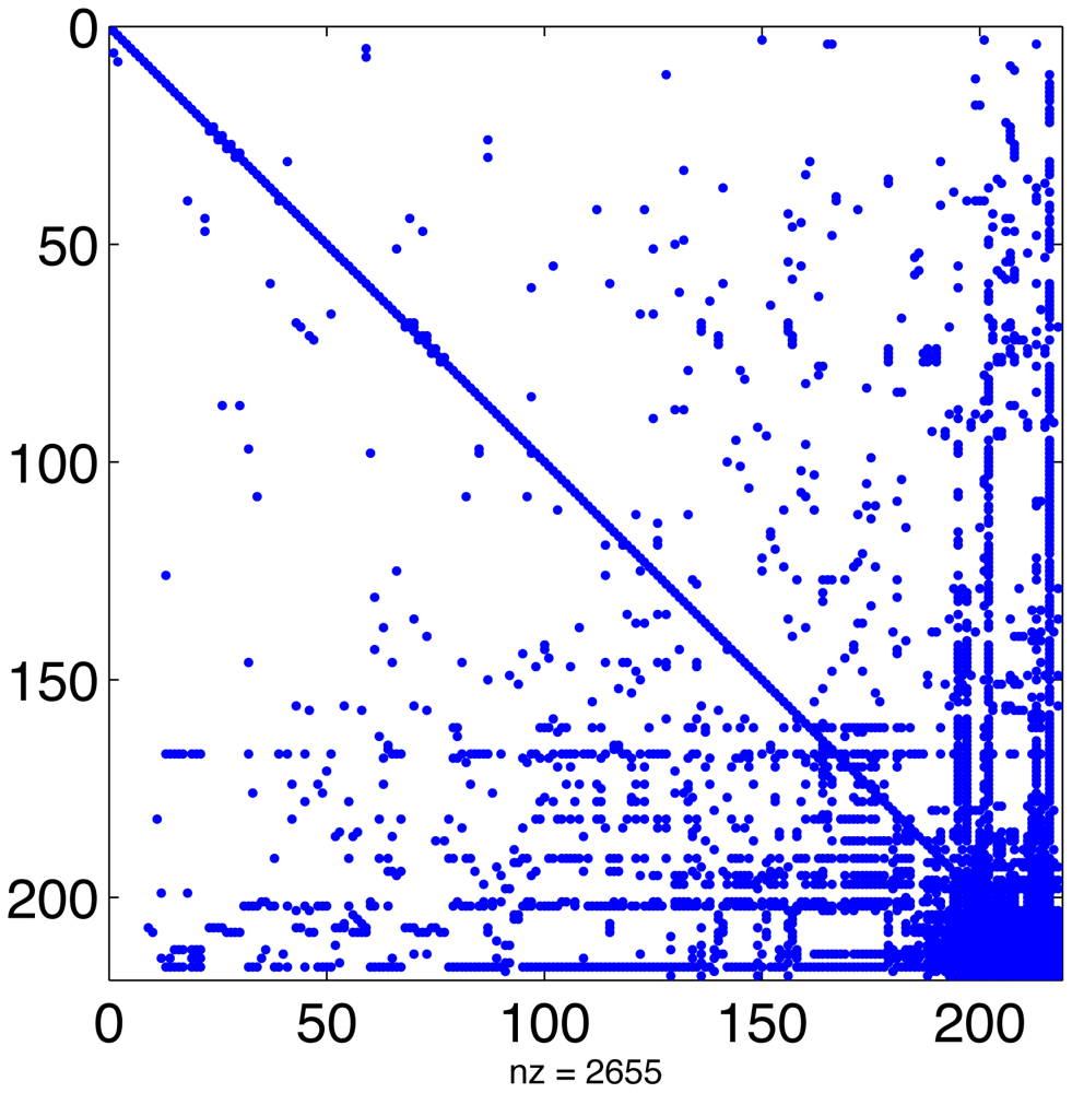
In a chemical kinetic solver, most of the computational effort is spent in solving the linear systems associated with the implicit time integration algorithms. For all methods discussed here the matrix of coefficients is of the form I − h γ J, and inherits the sparsity structure of the Jacobian.

In a typical chemical mechanism, the pattern of chemical interactions leads to a Jacobian that has the majority of entries equal to zero. Figure 1 displays the sparsity structure of the Jacobian of the MECCA chemical mechanism, used in the numerical experiments presented in Section 5. This Jacobian has 2655 nonzero entries, i.e., 5.6% of its total number of elements.

Linear algebra algorithms can take advantage of this to avoid unnecessary operations and greatly reduce CPU time. Since the sparsity structure depends only on the chemical network (and not on the values of concentrations or rate coefficients) it can be computed offline [22,61]. This approach has been taken by SMVGEAR [21] and by the Kinetic PreProcessor KPP [25]. KPP prepares highly efficient routines for sparse LU decomposition and substitution that are specific to the particular sparsity of the simulated chemical mechanism [24]. All stiff numerical methods implemented in the KPP library make use of these routines.

3.2. Acceleration Aspects

Recent developments inmulti-core chipset architectures canbe leveraged to reduce chemical simulation runtime. In general, good performance is achieved by using every tier of heterogeneous parallelism available to the model. Chemical kinetics are embarrassingly parallel between grid cells, so there is abundant data parallelism (DLP). Within the solver itself, the ODE system is coupled so that, while there is still some data parallelism available in lower-level linear algebra operations, parallelization is limited largely to the instruction level (ILP). (Some specific chemical mechanisms are only partially coupled and can be separated into a small number of sub-components, but such inter-module decomposition is rare.) Thus, a three-tier parallelization is possible: ILP on each core, DLP using single-instruction-multiple-data (SIMD) features of a single core, and DLP across multiple cores (using multi-threading) or nodes (using MPI). The coarsest tier of MPI and OpenMP parallelism is typically supplied by the atmospheric model.

This section presents parallelization strategies for Rosenbrock integration in one-cell-per-thread, N-cells-per-thread, and 4/2-cells-per-thread decompositions. For performance benchmarks of parallelized Rosenbrock solvers, see [32–34,62].

One-cell-per-thread (multi-threaded CPUs)

Although not an “accelerated” architecture, multi-threaded CPUs are common, inexpensive, and a mature target platform. Modest performance improvements are achievable by parallelizing the Rosenbrock integrator via OpenMP. Since the chemistry at each grid cell is independent, the outermost iteration over grid cells is thread-parallel dimension; that is, a one-cell-per-thread decomposition. Within the integrator itself, the inseparable Jacobian matrix prohibits direct parallelization, though SIMD instructions may be introduced by the compiler for a small intra-integrator performance improvement. The principal disadvantage of this architecture is a relatively low peak performance.

N-cells-per-thread (NVIDIA CUDA)

A CUDA implementation takes advantage of the high degree of parallelism and independence between cells in the simulation. The outermost loops of the solver are kept on the CPU and the GPU is used to accelerate the innermost computational kernels. Time loops, Runge-Kutta loops, and error control branch-back logic are executed on the CPU. LU decomposition and solve, the ODE function evaluation, Jacobi matrix operations, and BLAS operations, are coded and invoked as separate kernels on the GPU. All data for the solver is resident on the GPU and arrays are stored with cell-index stride-one so that adjacent threads access adjacent words in memory to coalesce access to the chemical data across threads. Under this paradigm, parallelism occurs within the solver across grid cells, rather than external to the solver and across grid cells as on a multi-core CPU. Although each GPU thread still processes only one cell, the exact mapping of threads to grid cells is handled by the GPU hardware, effectively achieving an N-cells-per-thread decomposition, where N is the total number of grid cells in the simulation.

This implementation is easy to debug and profile since the GPU code is spread over many small kernels with control returning frequently to the CPU. Additionally, resource bottlenecks such as register pressure and shared-memory usage are limited to only those affected kernels. Performance critical parameters such as the size of thread blocks and shared-memory allocation can be adjusted and tuned separately, kernel-by-kernel, without subjecting the entire solver to worst-case limits. One disadvantage is that all N grid cells are forced to use the minimum time step and iterate the maximum number of times, even though only a few cells will typically require that many iterations to converge. The overhead of these additional iterations can be mitigated by storing the per-cell time, time step length, and error in a vector and using vector masks to “turn off” cells that have converged. The solver still performs the maximum number of iterations, but thread-blocks assigned to cells that have converged do little or no work and relinquish the GPU cores quickly.

A CUDA implementation is straight-forward to program, but may prove difficult to optimize. CUDA's automatic thread management and familiar programming environment make solver implementations simple to conceive and implement. However, a deep understanding of the underlying architecture is required to achieve good performance. For example, memory access coalescing is one of the most powerful features of the GPU architecture, yet CUDA neither hinders nor promotes program designs that leverage coalescing. The principal limitation on performance is the size of the on-chip shared memory and register file, which prevent large-footprint applications from running sufficient numbers of threads to expose parallelism and hide latency to the device memory. In general, GPU implementations of the Rosenbrock solver are faster than multi-core CPU implementations, but by less than a factor of two. From a power consumption standpoint, this makes them less efficient than multi-core CPUs in this arena.

4/2-cells-per-thread (Cell Broadband Engine Architecture)

The heterogeneous Cell Broadband Engine Architecture can achieve exceptionally high levels of performance for the Rosenbrock integrator, yet its complexity and uniqueness make it difficult to program. As a heterogeneous architecture, a homogeneous one-cell-per-thread decomposition across all cores will not achieve maximum performance. A master-worker approach resulting in multiple grid cells processed per thread is more appropriate.

The Power Processing Element (PPE), with full access to main memory, is the master. It prepares the model data for processing by the Synergistic Processing Elements (SPEs) by padding and aligning data to comply with architectural restrictions. The Rosenbrock solver tends to be computation-bound, so the PPU has ample time to maintain a buffer of aligned data. The SPEs implement a 128-bit SIMD instruction set architecture. Hence, every cycle operates on 128-bit vectors of either four single precision or two double precision floating point numbers. The data of two or four grid cells, depending on floating point precision, are packaged together by the PPE into a single padded, aligned, and buffered payload for processing by the SPEs (a so-called “vector cell”). This achieves a four-cells-per-thread (two-cells-per-thread in double precision) decomposition.

A small change is required in the Rosenbrock integrator design to operate on a vector cell. Typically, the integrator iteratively refines the Newton step size h until the error norm is within acceptable limits. This will cause an intra-vector divergence if different vector elements accept different step sizes. However, it is numerically sound to continue to reduce h even after an acceptable step size is found. The vector cell integrator reduces the step size until the error for every vector element is within tolerance. Conventional architectures would require additional computation under this scheme, but because all operations in the SPE are SIMD this actually recovers lost flops. This enhancement doubles (quadruples for single precision) the SPE's throughput with no measurable overhead. Rosenbrock integrators on the Cell Broadband Engine Architecture tend to be about eight times faster than multi-core implementations on contemporary 8-core CPUs, and have regularly achieve speedups of 20-40× when compared to state-of-the-art Fortran implementations.

4. The Kinetic PreProcessor: KPP and KPPA

Writing chemical kinetics code is often tedious and error-prone work. The Kinetic PreProcessor (KPP) [25,41–45] is a general analysis tool that enables the rapidly generation of correct and efficient chemical kinetics code. The strength of KPP compared with other chemical processing tools such as SMVGEAR [21] lies in the integration of very efficient numerical analysis routines with its ability to automatically generate FORTRAN or C code that computes the time-evolution of chemical species from a specification of the chemical mechanism in KPP-Language (presented in detail in [25]). It also generates the Jacobian in either sparse or full format, as well as other objects needed by different numerical integration schemes. KPP provides a rich selection of numerical integration schemes including VODE, LSODES, RODAS, ROS4, SDIRK, SEULEX, QSSA, EXQSSA, RADAU5, RODAS3 and ROS3. The framework can be easily used as an accurate benchmarking platform for evaluating new integrators.

4.1. The Kinetic PreProcessor: Accelerated (KPPA)

KPP makes it possible to rapidly generate correct and efficient chemical kinetics solvers on scalar architectures, but these generated codes cannot be easily ported to multi-core accelerated or heterogeneous architectures. KPPA (the Kinetics PreProcessor: Accelerated) [32], is the next generation KPP tool that achieves significantly reduced time-to-solution for chemical kinetics kernels on both traditional and emerging architectures. In addition to the basic KPP functionality, KPPA generates OpenMP code with SSE or Alitivec for traditional CPUs, CUDA code for NVIDIA GPUs, and optimized C codes for the Cell Broadband Engine Architecture (CBEA), in either double or single precision. KPPA-generated mechanisms leverage platform-specific multi-layered heterogeneous parallelism to achieve strong scalability. Compared to state-of-the-art serial implementations, speedups of 20×–40× are regularly observed in KPPA-generated code.

KPPA combines a general analysis tool for chemical kinetics with a code generation system for scalar, homogeneous multi-core, and heterogeneous multi-core architectures. It is written in object-oriented C++ with a clearly-defined upgrade path to support future multi-core architectures as they emerge. KPPA has all the functionality of KPP 2.1 and maintains backwards compatibility with KPP. Many atmospheric models, including WRF-Chem and STEM, support a number of chemical kinetics solvers that are automatically generated at compile time by KPP. Reusing these analysis techniques in KPPA insures its accuracy and applicability.

KPPA's code generation component accommodates a two-dimensional design space of programming language/target architecture combinations superseding the one-dimensional design space of KPP (

Table 2. Language/architecture combinations supported by KPP and KPPA. κ denotes functionality found only in KPPA.

	Serial	OpenMP	GPGPU	CBEA
C	KPP	k	k	k
FORTRAN77	KPP	k		k
Fortran 90	KPP	k		k
MATLAB	KPP

). Given the model description from the analytical component and a description of the target architecture, the code generation component produces a time-stepping integrator, the ODE function and ODE Jacobian of the system, and other quantities required to interface with an atmospheric model.

KPPA's key feature is its ability to generate fully-unrolled, platform-specific sparse matrix/matrix and matrix/vector operations that achieve very high levels of efficiency. As KPPA parses it's input, language independent expression trees describing sparse matrix/matrix or matrix/vector operations are constructed in memory. For example, the aggregate ODE function of the chemical mechanism is calculated by multiplying the left-side stoichiometric matrix by the concentration vector, and then adding the result to elements of the stoichiometric matrix. KPPA performs these operations symbolically at code generation time, using the matrix formed by the analytical component and a symbolic vector, which will be calculated at run-time. The result is an expression tree of language-independent arithmetic operations and assignments, equivalent to a rolled-loop sparse matrix/vector operation, but in completely unrolled form.

KPPA uses its knowledge of the target architecture to generate highly-efficient code from the expression tree. Vector types are preferred when available, branches are avoided on all architectures, and parts of the function can be rolled into a tight loop if KPPA determines that on-chip memory is a premium. An analysis of four KPPA-generated ODE functions and ODE Jacobians targeting the CBEA showed that, on average, both SPU pipelines remain full for over 80% of the function implementation. Pipeline stalls account for less than 1% of the cycles required to calculate the function. For example, in the SAPRCNOV mechanism on CBEA, there are only 20 stalls in the 2989 cycles required by the ODE function (0.66%), and only 24 stalls in the 5490 cycles required for the ODE Jacobian (0.43%). Code of this caliber typically requires meticulous hand-optimization, but KPPA is able to generate this code automatically in seconds. See [32] for further performance analysis of KPPA.

5. Numerical Results

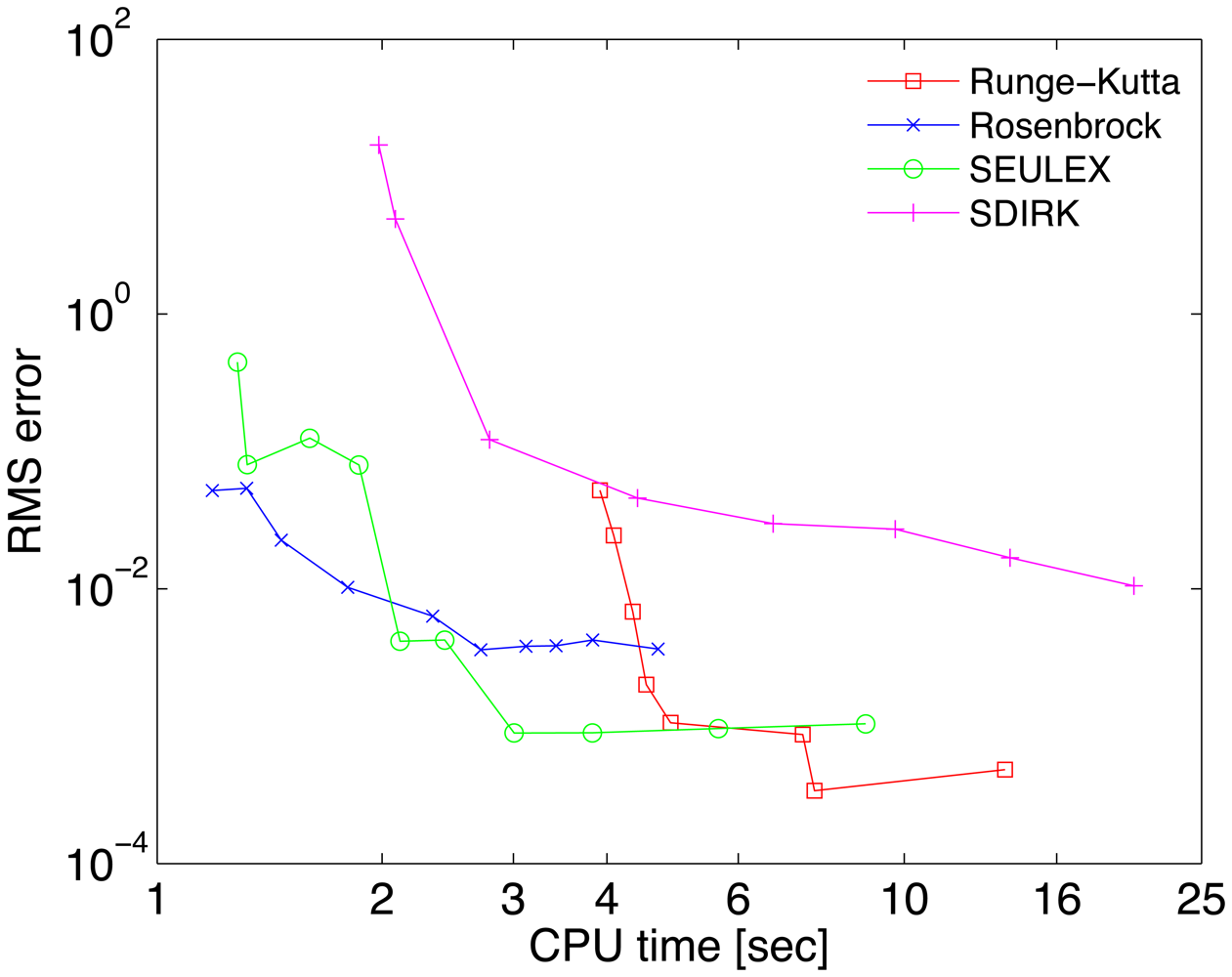
For the numerical results we use the CAABA box model with MECCA chemistry [63]. A mechanism suitable for calculating marine boundary layer chemistry containing 223 species and 560 reactions in the gas phase and in aerosol particles was selected. In addition to the basic atmospheric chemistry of ozone, methane, HO_x and NO_x, halogen (Cl, Br, I) and sulfur chemistry are also considered. The full mechanism including rate coefficients can be found in the supplement.

A reference solution y^ref has been computed with the Radau-5A numerical method implemented in the KPP Runge Kutta suite, with the tight tolerances RelTol = 10⁻¹⁰ and AbsTol = 10² molecules/cm³. The accuracy of each numerical solution is measured by its RMS error, defined as

$$\text{RMS}=\sqrt{\frac{{\sum }_{i=1}^d{\left(\frac{y_i-y_i^{\text{ref}}}{y_i^{\text{ref}}}\right)}^2\cdot (y_i^{\text{ref}}\ge \text{threshold})}{{\sum }_{i=1}^d(y_i^{\text{ref}}\ge \text{threshold})}}$$

(27)

The threshold value is 100 molecules/cm³. The logical expression Darshana takes a value equal to one if the reference concentration of the i-th species is above the threshold, and takes the value zero otherwise. Thus only those species for which concentrations are sufficiently large contribute to the error metric Equation (27).

The work-precision diagrams for several numerical integrators are shown in Figure 2. The RMS errors Equation (27) of different solutions at the final time are plotted against the CPU effort needed to obtain them. Each curve corresponds to a different method. Several relative tolerances in the range RelTol ∈ [10⁻⁶, 10⁻¹] have been used to generate different points on each curve.

6. Conclusions

One of the most computationally demanding tasks in atmospheric chemical transport simulations is the solution of chemical kinetic processes. Special considerations need to be taken into account when designing chemistry time integration algorithms. Unconditionally stable methods are needed due to the stiff nature of the equations; such algorithms perform expensive solves of (non)linear systems of equations at each stage. The accuracy requirements are relatively low, with relative errors of 0.1%, but compute times must be low as well. This is achieved with algorithms that quickly adjust time step size, and efficient step size control mechanisms. A challenge comes from the fact that error estimators based on asymptotic formulas may not work well in the low accuracy regime. Closed chemical systems preserve mass and charge, and the concentrations remain positive. It is desirable to have numerical solvers that also preserve this properties. Conservation is easy to achieve, but positivity requires more involved computations.

Several families of solvers that are suitable for atmospheric chemical kinetics were discussed: QSSA, BDF, implicit Runge-Kutta, Rosenbrock, and Extrapolation. Special implementations of general purpose methods have taken the place of special integrators (e.g., QSSA) during the last decade. Among them the Rosenbrock methods have become popular due to their efficiency at moderate accuracy requirements.

A major goal when implementing a chemical solver is efficiency, since many copies of the chemical mechanism (one per grid cell) need to be solved at each operator split cycle. Careful exploitation of the Jacobian structure and the use of efficient sparse linear algebra operations are key to obtaining efficiency. The ideal parallelism between the chemical tasks in different grid cells can be exploited either by domain decomposition, or by vectorization. The latter approach has found renewed interest in the context of of modern heterogeneous multicore (accelerator) architectures.

All the numerical methods discussed in this paper are implemented in the KPP numerical library [64] and can be easily employed in applications. KPP prepares efficient sparse linear algebra routines that are specific to the structure of the system at hand. KPPA [65] is able to automatically generate code for accelerator architectures such as the IBM Cell Broadband Engine Architecture and general purpose graphical units.

With the increase in complexity of gas phase chemical mechanisms, and the frequent inclusion of aqueous and heterogeneous phase chemistry in three dimensional simulations, the importance of efficient and robust solvers for atmospheric chemistry models is expected to continue to increase in future.

Supplementary Material

atmosphere-02-00510-s001.pdf

References

- Yanenko, N.N. The Method of Fractional Steps; Springer-Verlag: Berlin, Heidelberg, Germany, 1971. [Google Scholar]
- Verwer, J.; Hunsdorfer, W.; Blom, J.G. Numerical Time Integration of Air Pollution Models; Modeling, Analysis and Simulations report MAS-R9825; CWI: Amsterdam, The Netherlands; October; 1998. [Google Scholar]
- Sandu, A.; Daescu, D.; Carmichael, G.; Chai, T. Adjoint sensitivity analysis of regional air quality models. J. Comput. Phys. 2005, 204, 222–252. [Google Scholar]
- Chai, T.; Carmichael, G.; Tang, Y.; Sandu, A.; Hardesty, M.; Pilewskie, P.; Whitlow, S.; Browell, E.; Avery, M.; Thouret, V.; et al. Four dimensional data assimilation experiments with ICARTT (International Consortium for Atmospheric Transport and Transformation) ozone measurements. J. Geophys. Res. 2007, 112. [Google Scholar] [CrossRef]
- Constantinescu, E.; Sandu, A.; Chai, T.; Carmichael, G. Autoregressive models of background errors for chemical data assimilation. J. Geophys. Res. 2007, 112. [Google Scholar] [CrossRef]
- Sandu, A.; Zhang, L. Discrete second order adjoints in atmospheric chemical transport modeling. J. Comput. Phys. 2008, 227, 5949–5983. [Google Scholar]
- Constantinescu, E.; Sandu, A.; Chai, T.; Carmichael, G. Assessment of ensemble-based chemical data assimilation in an idealized setting. Atmos. Environ. 2007, 41, 18–36. [Google Scholar]
- Constantinescu, E.; Sandu, A.; Chai, T.; Carmichael, G. Ensemble-based chemical data assimilation. I: General approach. Q. J. R. Meteorol. Soc. 2007, 133, 1229–1243. [Google Scholar]
- Constantinescu, E.; Sandu, A.; Chai, T.; Carmichael, G. Ensemble-based chemical data assimilation. II: Covariance localization. Q. J. R. Meteorol. Soc. 2007, 133, 1245–1256. [Google Scholar]
- Carmichael, G.; Chai, T.; Sandu, A.; Constantinescu, E.; Daescu, D. Predicting air quality: Improvements through advanced methods to integrate models and measurements. J. Comput. Phys. 2008, 227, 3540–3571. [Google Scholar]
- Zhang, L.; Constantinescu, E.; Sandu, A.; Tang, Y.; Chai, T.; Carmichael, G.; Byun, D.; Olaguer, E. An adjoint sensitivity analysis and 4D-Var data assimilation study of Texas air quality. Atmos. Environ. 2008, 42, 5787–5804. [Google Scholar]
- Singh, K.; Eller, P.; Sandu, A.; Henze, D.; Bowman, K.; Kopacz, M.; Lee, M. Towards the Construction of a Standard Adjoint GEOS-Chem Model. Proceedings of the 2009 Spring Simulation Multiconference (SpringSim'09), High Performance Computing Symposium (HPCS-2009), San Diego, CA, USA, 22–27 March 2009; Ribbens, C., Sandu, A., Thacker, W., Eds.; Society for Modeling and Simulation International (SCS)/ACM: San Diego, CA, USA; New York, NY, USA, 2009; p. 8. [Google Scholar]
- Hakami, A.; Henze, D.; Seinfeld, J.; Chai, T.; Tang, Y.; Carmichael, G.; Sandu, A. Adjoint inverse modeling of black carbon during ACE-Asia. J. Geophys. Res. 2005, 110, D14301. [Google Scholar]
- Hakami, A.; Henze, D.; Seinfeld, J.; Singh, K.; Sandu, A.; Kim, S.; Byun, D.; Li, Q. The adjoint of CMAQ. Environ. Sci. Technol. 2007, 41, 7807–7817. [Google Scholar]
- Hairer, E.; Norsett, S.; Wanner, G. Solving Ordinary Differential Equations II. Stiff and Differential-Algebraic Problems/E, 2nd ed.; Springer-Verlag: Berlin, Germany, 2002; Volume 2. [Google Scholar]
- Rosenbaum, J. Conservation properties of numerical integration methods for systems of ordinary differential equations. J. Comput. Phys. 1976, 20, 259–267. [Google Scholar]
- Bolley, C.; Crouzeix, M. Conservation de la positivite lors de la discretization des problemes d'evolution parabolique. R.A.I.R.O. Numer. Anal. 1978, 12, 237–245. [Google Scholar]
- Sandu, A. Positive numerical integration methods for chemical kinetic systems. J. Comput. Phys. 2001, 170, 1–14. [Google Scholar]
- Sandu, A. Time-Stepping Methods that Favor Positivity for Atmospheric Chemistry Modeling. In IMA Volume on Atmospheric Modeling; Chock, D., Carmichael, G., Eds.; Springer-Verlag: Berlin, Germany, 2001; pp. 1–21. [Google Scholar]
- Jay, L.O.; Sandu, A.; Potra, F.A.; Carmichael, G.R. Improved QSSA methods for atmospheric chemistry integration. SIAM J. Sci. Comp. 1997, 18, 182–202. [Google Scholar]
- Jacobson, M.Z.; Turco, R. SMVGEAR: A sparse-matrix, vectorized Gear code for atmospheric models. Atmos. Environ. 1994, 17, 273–284. [Google Scholar]
- Sandu, A.; Potra, F.; Damian-Iordache, V.; Carmichael, G. Efficient implementation of fully implicit methods for atmospheric chemistry. J. Comput. Phys. 1996, 129, 101–110. [Google Scholar]
- Sandu, A.; Verwer, J.; Blom, J.; Spee, E.; Carmichael, G.; Potra, F. Benchmarking stiff ODE solvers for atmospheric chemistry problems. II: Rosenbrock methods. Atmos. Environ. 1997, 31, 3459–3472. [Google Scholar]
- Sandu, A.; Verwer, J.; van Loon, M.; Carmichael, G.; Potra, F.; Dabdub, D.; Seinfeld, J. Benchmarking stiff ODE solvers for atmospheric chemistry problems. I: Implicit versus explicit. Atmos. Environ. 1997, 31, 3151–3166. [Google Scholar]
- Damian, V.; Sandu, A.; Damian, M.; Potra, F.; Carmichael, G. The Kinetic PreProcessor KPP—A software environment for solving chemical kinetics. Comput. Chem. Eng. 2002, 26, 1567–1579. [Google Scholar]
- Foster, I. Designing and Building Parallel Programs; Addison-Wesley: Boston, MA, USA, 1995. [Google Scholar]
- Miehe, P.; Sandu, A.; Carmichael, G.; Tang, Y.; Daescu, D. A communication library for the parallelization of air quality models on structured grids. Atmos. Environ. 2002, 36, 3917–3930. [Google Scholar]
- Belwal, C.; Sandu, A.; Constantinescu, E. Parallel Adaptive Simulations of Regional Air Quality. Proceedings of the SIAM Conference on Parallel Processing PP04, San Francisco, CA, USA, 28 February 2004.
- Belwal, C.; Sandu, A.; Constantinescu, E. Adaptive Resolution Modeling of Air Pollution., Proceedings of the ACM Symposium on Applied Computing (SAC-2004), Nicosia, Cyprus, 14–17 March 2004; pp. 235–239.
- Sandu, A.; Daescu, D.; Carmichael, G.; Chai, T. Parallel Chemical Data Assimilation in Atmospheric Models. Proceedings of the SIAM Conference on Parallel Processing PP04, San Francisco, CA, USA, 25–27 February 2004.
- Sandu, A.; Belwal, C.; Constantinescu, E. Parallel Adaptive Simulations of Regional Air Quality. Proceedings of the SIAM Conference on Parallel Processing for Scientific Computing, Seattle, WA, USA, 24–26 Fabruary 2004.
- Linford, J.C.; Michalakes, J.; Vachharajani, M.; Sandu, A. Automatic generation of multicore chemical kernels. IEEE TPDS 2011, 22, 119–131. [Google Scholar]
- Linford, J.C.; Sandu, A. Scalable heterogeneous parallelism for atmospheric modeling and simulation. J. Supercomput. 2011, 56, 300–327. [Google Scholar]
- Linford, J.C.; Michalakes, J.; Vachharijani, M.; Sandu, A. Multi-Core Acceleration of Chemical Kinetics for Modeling and Simulation. Proceedings of the 2009 ACM/IEEE Conference on Supercomputing (SC'09), Portland, OR, USA, November 2009.
- Jöckel, P.; Kerkweg, A.; Pozzer, A.; Sander, R.; Tost, H.; Riede, H.; Baumgaertner, A.; Gromov, S.; Kern, B. Development cycle 2 of the Modular Earth Submodel System (MESSy2). Geosci. Model Dev. 2010, 3, pp. 717–752. Available online: http://www.geosci-model-dev.net/3/717 (accessed on 2 September 2011). [Google Scholar]
- Chapman, S. On ozone and atomic oxygen in the upper atmosphere. Phil. Mag. 1930, 10, 369–383. [Google Scholar]
- Bates, D.R.; Nicolet, M. The photochemistry of atmospheric water vapor. J. Geophys. Res. 1950, 55, 301–327. [Google Scholar]
- Hunt, B.G. Photochemistry of ozone in a moist atmosphere. J. Geophys. Res. 1966, 71, 1385–1398. [Google Scholar]
- Shimazaki, T.; Laird, A.R. A model calculation of the diurnal variation in minor neutral constituents in the mesosphere and lower thermosphere including transport effects. J. Geophys. Res. 1970, 75, 3221. [Google Scholar]
- Turco, R.P.; Whitten, R.C. A comparison of several computational techniques for solving some common aeronomic problems. J. Geophys. Res. 1974, 79, 3179–3185. [Google Scholar]
- Sandu, A.; Miehe, P. Forward, tangent linear, and adjoint Runge Kutta methods in KPP-2.2 for efficient chemical kinetic simulations. Int. J. Comp. Math. 2010, 87, 2458–2479. [Google Scholar]
- Eller, P.; Singh, K.; Sandu, A.; Bowman, K.; Henze, D.; Lee, M. Implementation and evaluation of an array of chemical solvers in a global chemical transport model. Geophys. Model Dev. 2009, 2, 1–7. [Google Scholar]
- Sandu, A.; Sander, R. Modeling chemical kinetic systems in Fortran90 and Matlab with KPP-2.1. Atmos. Chem. Phys. 2006, 6, 187–195. [Google Scholar]
- Daescu, D.; Sandu, A.; Carmichael, G. Direct and adjoint sensitivity analysis of chemical kinetic systems with KPP: II—Numerical validation and applications. Atmos. Environ. 2003, 37, 5097–5114. [Google Scholar]
- Sandu, A.; Daescu, D.; Carmichael, G. Direct and adjoint sensitivity analysis of chemical kinetic systems with KPP: I —Theory and software tools. Atmos. Environ. 2003, 37, 5083–5096. [Google Scholar]
- Community Multiscale Air Quality (CMAQ) modeling system. Available online: http://www.cmaq-model.org (accessed on 5 May 2011).
- Goddard Earth Observing System (GEOS)-Chem. Available online: http://acmg.seas.harvard.edu/geos (accessed on 5 May 2011).
- Sulphur Transport Eulerian Model (STEM). Available online: http://cgrer.uiowa.edu/projects (accessed on 5 May 2011).
- 5th generation of European Centre Hamburg Model/Modular Earth Submodel System (ECHAM5/MESSy). Available online: http://www.messy-interface.org (accessed on 5 May 2011).
- Weather Research and Forecasting model coupled with Chemistry (WRF-Chem). Available online: http://www.acd.ucar.edu/wrf-chem (accessed on 5 May 2011).
- Hesstvedt, E.; Hov, O.; Isaacsen, I. Quasi-steady-state-approximation in air pollution modelling: comparison of two numerical schemes for oxidant prediction. Int. J. Chem. Kinet. 1978, 10, 971–994. [Google Scholar]
- Hochbruck, M.; Lubich, C.; Selhofer, H. Exponential integrators for large systems of differential equations. SIAM J. Sci. Comput. 1998, 19, 1552–1574. [Google Scholar]
- Radhakrishnan, K.; Hindmarsh, A. Description and Use of LSODE, the Livermore Solver for Ordinary Differential Equations.; Report UCRL-ID-113855; Lawrence Livermore National Laboratory: Livermore, CA, USA, 1993. [Google Scholar]
- Brown, P.; Byrne, G.; Hindmarsh, A. VODE: A variable step ODE solver. SIAM J. Sci. Stat. Comput. 1989, 10, 1038–1051. [Google Scholar]
- Hindmarsh, A.C.; Brown, P.N.; Grant, K.E.; Lee, S.L.; Serban, R.; Shumaker, D.E.; Woodward, C.S. SUNDIALS: Suite of nonlinear and differential/algebraic equation solvers. ACM Trans. Math. Softw. 2005, 31, 363–396. [Google Scholar]
- Gear, C.W. Numerical Initial Value Problems in Ordinary Differential Equations; Prentice Hall PTR: Upper Saddle River, NJ, USA, 1971. [Google Scholar]
- Jacobson, M.Z. Vecotr and scalar improvement of SMVGEAR II through absolute error tolerance control. Atmos. Environ. 1998, 32, 791–796. [Google Scholar]
- Rosenbrock, H.H. Some general implicit processes for the numerical solution of differential equations. Comput. J. 1963, 5, 329–330. [Google Scholar]
- Carmichael, G.; Sandu, A.; Potra, F.; Damian-Iordache, V.; Damian-Iordache, M. The current state and the future directions in air quality modeling. Syst. Anal. Model. Simul. 1996, 25, 75–105. [Google Scholar]
- Hairer, E.; Norsett, S.; Wanner, G. Solving Ordinary Differential Equations I. Nonstiff Problems; Springer-Verlag: Berlin, Germany, 1993. [Google Scholar]
- Jay, L.; Sandu, A.; Potra, F.; Carmichael, G. Efficient Numerical Integration for Atmospheric Chemistry. Proceedings of the 3rd International Congress on Industrial and Applied Mathematics (ICIAM-1995); Hamburg, Germany, 3-7 July 1995; Kreuzer, E., Mahrenholtz, O., Eds.; pp. 450–453.
- Linford, J.C.; Sandu, A. Chemical Kinetics on Multi-core SIMD Architectures. Proceedings of the 9th Internation Conference on Computational Science—ICCS 2009, Baton Rouge, LA, USA, 25-27 May 2009; Allen, G., Nabrzyski, J., Seidel, E., van Albada, G.D., Dongarra, J., Sloot, P.M., Eds.; Springer: Hoboken, NJ, USA, 2009; 5544. [Google Scholar]
- Sander, R.; Baumgaertner, A.; Gromov, S.; Harder, H.; Jöckel, P.; Kerkweg, A.; Kubistin, D.; Regelin, E.; Riede, H.; Sandu, A.; Taraborrelli, D.; Tost, H.; Xie, Z.Q. The atmospheric chemistry box model CAABA/MECCA-3.0. Geosci. Model Dev. 2011, 4, pp. 373–380. Available online: http://www.geosci-model-dev.net/4/373 (accessed on 5 May 2011). [Google Scholar]
- Kinetic PreProcessor (KPP). Available online: http://www.cs.vt.edu/∼asandu/Software/Kpp (accessed on 5 May 2011).
- Kinetic PreProcessor : Accelerated (KPPA). Available online http://code.google.com/p/kppa/ (accessed on 5 May 2011).
- ‡The paper is dedicated to the memory of Dr. Daewon Byun, whose work remains a lasting legacy to the field of air quality modeling and simulation.
© 2011 by the authors; licensee MDPI, Basel, Switzerland. This article is an open access article distributed under the terms and conditions of the Creative Commons Attribution license (http://creativecommons.org/licenses/by/3.0/).
Share and Cite
Zhang, H.; Linford, J.C.; Sandu, A.; Sander, R. Chemical Mechanism Solvers in Air Quality Models. Atmosphere 2011, 2, 510-532. https://doi.org/10.3390/atmos2030510
Zhang H, Linford JC, Sandu A, Sander R. Chemical Mechanism Solvers in Air Quality Models. Atmosphere. 2011; 2(3):510-532. https://doi.org/10.3390/atmos2030510
Chicago/Turabian StyleZhang, Hong, John C. Linford, Adrian Sandu, and Rolf Sander. 2011. "Chemical Mechanism Solvers in Air Quality Models" Atmosphere 2, no. 3: 510-532. https://doi.org/10.3390/atmos2030510