Article

The Impact of Uncertainties in African Biomass Burning Emission Estimates on Modeling Global Air Quality, Long Range Transport and Tropospheric Chemical Lifetimes

by
Jason E. Williams
1,*,
Michiel van Weele
1,
Peter F. J. van Velthoven
1,
Marinus P. Scheele
1,
Catherine Liousse
2 and
Guido R. van der Werf
3
1
Chemistry and Climate Division, Royal Netherlands Institute (KNMI), P.O. Box 201, De Bilt 3730 AE, The Netherlands
2
Laboratoire d’Aerologie, UMR 5560, 31400 Toulouse, France
3
Department of Hydrology and Geo-Environmental Sciences, Faculty of Earth and Life Sciences, Vrije Universiteit, Amsterdam 1081 HV, The Netherlands
*
Author to whom correspondence should be addressed.
Atmosphere 2012, 3(1), 132-163; https://doi.org/10.3390/atmos3010132
Submission received: 25 December 2011 / Revised: 19 January 2012 / Accepted: 19 January 2012 / Published: 9 February 2012
(This article belongs to the Special Issue Biomass Emissions)

Abstract

:
The chemical composition of the troposphere in the tropics and Southern Hemisphere (SH) is significantly influenced by gaseous emissions released from African biomass burning (BB). Here we investigate how various emission estimates given in bottom-up BB inventories (GFEDv2, GFEDv3, AMMABB) affect simulations of global tropospheric composition using the TM4 chemistry transport model. The application of various model parameterizations for introducing such emissions is also investigated. There are perturbations in near-surface ozone (O3) and carbon monoxide (CO) of ~60–90% in the tropics and ~5–10% in the SH between different inventories. Increasing the update frequency of the temporal distribution to eight days generally results in decreases of between ~5 and 10% in near-surface mixing ratios throughout the tropics, which is larger than the influence of increasing the injection heights at which BB emissions are introduced. There are also associated differences in the long range transport of pollutants throughout the SH, where the composition of the free troposphere in the SH is sensitive to the chosen BB inventory. Analysis of the chemical budget terms reveals that the influence of increasing the tropospheric CO burden due to BB on oxidative capacity of the troposphere is mitigated by the associated increase in NOx emissions (and thus O3) with the variations in the CO/N ratio between inventories being low. For all inventories there is a decrease in the tropospheric chemical lifetime of methane of between 0.4 and 0.8% regardless of the CO emitted from African BB. This has implications for assessing the effect of inter-annual variability in BB on the annual growth rate of methane.

1. Introduction

The release of large quantities of trace gas pollutants into the tropical troposphere from human burning practices and wildfires in Africa exerts a significant influence on global atmospheric composition, most importantly on the relatively pristine Southern Hemisphere (SH), tropical Atlantic [1,2,3] and around the burning regions. The resulting emissions from biomass burning (BB) impact directly on air quality by reducing visibility with concurrent enhancement in aerosol concentrations and associated reduction in photochemical activity. It has also been shown that the long range transport of pollutants emitted from BB can affect air quality thousands of kilometers away from the source [4]. It is estimated that open burning in Africa accounts for more than 50% of the total global BB emissions during any typical year [5,6]. It is therefore important to quantify the sensitivity of SH atmospheric composition to the uncertainty associated with African BB emission estimates.
The large interannual variability in the timing, distribution and extent of burning events can presently be mapped by making use of satellite observations and using the total burned area products [6,7,8,9]. To quantify the strength of the emission sources methodologies have been developed which combine such satellite observations with, e.g., terrestrial ecosystem models that account for differences in both land type and the availability of biomass for burning. This has lead to the development of a number of bottom-up emission inventories for use in three-dimensional global chemistry-transport models (3D global CTMs) [6,8,9]. A recent intercomparison of BB emission inventories for the year 2003 has highlighted large differences in both the seasonality and the total flux of gases emitted from tropical burning regions [10]. This study concluded that no preference can be given towards which methodology captures BB events most accurately, where there are both seasonal and regional differences in the performance of each inventory. This introduces significant uncertainty in the associated emissions of CO, nitrogen oxides (NOx), non-methane hydrocarbons (NMHCs) and carbonaceous aerosols from BB emission sources. Thus, the most advanced bottom-up BB inventories that are currently available for use in 3D global CTMs exhibit significant differences in the integrated seasonal fluxes.
The strong convective uplift of BB emissions due to the increased air buoyancy above fires means that BB emissions exhibit a vertical injection profile that is commonly accounted for in 3D global CTMs [11]. The vertical distribution can be constrained using statistical composites derived using satellite measurements [12], with injection heights being dependant on the cumulative effects of fire intensity, land type, season and the local meteorological parameters. Although BB emissions in the tropics are rarely injected directly into the free troposphere (FT) [13,14], the long range transport out of the main burning regions can be influenced by the method with which BB emissions are introduced into large-scale atmospheric models [3]. Therefore, the description of BB emissions in global CTMs may have consequences concerning the fraction of the emitted species transported away from the source regions and the subsequent conclusions drawn as to the importance of African BB for the chemical composition of the troposphere in the tropics and SH.
Typical applications of 3D global CTMs include: (i) the quantification of the long range transport of pollutants between continents and more remote locations; (ii) the investigation of chemical source-receptor relationships; and (iii) the provision of estimates of the atmospheric lifetimes of key trace gases such as CO (τCO), O3 (τO3) and CH4 (τCH4). Recent multi-model intercomparison studies estimate that in large-scale global models τCO, τO3 and τCH4 have typical values of ~2 months, ~22 days and ~8.7 years, respectively [15,16]. These chemical lifetimes control the impact of emission sources on air quality far away from the source area by changing the resident surface concentrations [17]. Moreover, any increases in the global burdens of the greenhouse gases CH4 and O3 impact on climate due to their warming potential. Such warming has the potential to induce a positive feedback on wildfire incidence via more frequent drought conditions [18].
The removal of CO and CH4 is principally governed by the resident concentration of the OH radical formed via the photolysis of O3 in the presence of H2O, where O3 is efficiently regenerated in the presence of NOx and sunlight. A chemical budget analysis from a typical CTM simulation reveals that CO and CH4 scavenge ~40% and ~16% of the available global OH in the troposphere, respectively, with a large fraction of the oxidation occurring in the tropics (30°S–30°N). The impacts of BB emissions on τCH4 are manifold, with the net impact being rather uncertain. For instance, in response to the widespread 1997 Indonesian wildfires, Duncan et al. [19] have shown that τCH4 increases due to large-scale reductions in OH (>20%). This reduction was ascribed to enhanced CO emissions released from the fires, enhanced heterogeneous loss of HOx radicals and reductions in UV light caused by increases in BB aerosols. However other more recent studies have suggested that the observed increase in CH4 during 1997 measured by the NOAA Earth System Research Laboratory (ESRL) surface monitoring network was due to enhanced CH4 emissions directly from increased BB rather than due to increased competition for OH [20]. Other studies suggest a combination of both CH4 emissions and lifetime changes to explain the variable annual growth rate [21]. Also the anomalous climatic conditions that favour intensive BB events result in a dry, arid environment with reduced cloudiness, which impact OH, O3 (via lower biogenic and BB NOx), τCO and τCH4.
For anthropogenic emissions it has been shown that the global OH distribution, and thus τCH4, is significantly affected by the ratio of CO and N (as nitrogen oxides) emitted into the atmosphere [22,23]. For BB the CO/N ratio is typically much higher than anthropogenic emissions due to incomplete combustion processes [23]. This has the potential to impact the global CO burden, and thus τCH4, due to a lower fraction of the emitted CO being oxidized in/around the source region. To date to our knowledge there has been no similar investigation as to how the potential variability in the CO/N ratio from BB emission inventories impacts on the atmospheric lifetimes of abundant trace gases when applied in a global CTM, which is a major focus of this study.
In this paper we investigate the uncertainties introduced towards simulating global tropospheric composition associated with differences between bottom-up BB emission estimates when applied in a global 3D CTM. For this purpose we examine the influence on global air quality, the long range transport of pollutants out of BB source regions and the perturbations introduced in estimating global atmospheric lifetimes of dominant trace species. We also investigate the impact of increasing the update frequency with respect to the temporal distribution of BB emissions and the parameterization used for introducing tropical BB emission into the boundary layer on both tropical and SH composition. Finally we show that there is a compensating effect towards the perturbations introduced towards the oxidative capacity of the troposphere due to the CO/N ratio defined in different BB emission inventories, which constrains the effects on the global lifetimes for dominant trace gases.

2. Model Simulations and Emissions

The global 3D CTM used for this study is TM4, where the version applied here has been comprehensively described elsewhere [3]. The model is run at a horizontal resolution of 3° × 2° using 34 vertical levels with a model top of 0.1 hPa and is driven by meteorological fields from the European Centre for Medium-Range Weather Forecasting (ECMWF) operational analysis. The model uses the modified CBM4 chemical mechanism [24] updated to include recent recommendations to the reaction rate data [25]. Photolysis rates are calculated using the parameterization of Landgraf and Crutzen [26], modified to account for attenuation effects by clouds and ground albedo [27]. The chosen simulation year is 2006, for which the distribution of both CO and O3 in TM4 have recently been evaluated against a host of different measurements taken in and around the African continent [3,28,29] and where burning intensity in Africa is representative of a typical year [6]. For global anthropogenic and biogenic emissions we use the emission inventories provided by the EU-RETRO project for the year 2000 (http://retro.enes.org).
In this study we principally focus on differences between BB inventories provided for the African domain (here defined as the region 34°S–34°N, 20°W–40°E). BB emission estimates are taken from bottom-up BB inventories, namely: GFEDv2 [8], GFEDv3 [6], and AMMABB [9], for which large differences have been shown to exist in the emission estimates for both trace gases and aerosols [9,10]. For regions outside the African domain we adopt the GFEDv2 emission inventory for BB in all simulations. The update frequency of these inventories is monthly, where the original inventories are provided on either a 1° × 1° or 0.5° × 0.5° grid resolution and subsequently coarsened for application in TM4. To account for typical burning practises a daily burning cycle is applied to all BB emissions over the latitudinal range 20°S–20°N peaking at 2 pm local time [30]. For the majority of simulations BB emissions between 20°S–20°N are introduced into the first 2 km of the troposphere, with ~50% being placed between 0 and 1 km and ~50% being placed between 1 and 2 km. For the mid- and high latitudes, burning heights are adopted from the literature [11]. To quantify the global impact of African BB emissions on both long range transport and the atmospheric burdens and lifetimes of dominant trace species we perform a simulation where African BB emissions are turned off (referred to as NONE). In all simulations the CH4 surface concentrations are constrained by relaxation towards observations made at pristine locations as part of the NOAA surface network. This allows TM4 to capture the latitudinal gradient and seasonal cycles which are present, as well as the variability in the CH4 growth rate over recent decades [20]. Therefore differences in the estimates of direct CH4 emissions from BB are not accounted for in this study, although these are rather small typically ranging between 17 and 20 Tg CH4 yr−1 [6,8]. In these simulations a CH4 surface gradient exists of ~1,770 ppb at 35°S and ~1,850 ppb at 35°N. A one year spin-up period is adopted for all simulations using the relevant BB emission inventory available for the year 2005.
Table 1. A definition of the sensitivity simulations conducted in this study. These different emission inventories are applied for the African domain only. All other regions use GFEDv2 monthly estimates with latitudinally dependant injection heights from Dentener et al. [11].
Definition of SimulationBiomass Burning Emission InventoryInjection Height (km)Temporal Update Frequency
GFEDv2GFEDv20–2Monthly
GFEDv3GFEDv30–2Monthly
AMMABBAMMABB0–2Monthly
AMMABB_LOWNOXAMMABB0–2Monthly
8DAYGFEDv20–28-day
HIGH-IHGFEDv20–3Monthly
Sensitivity studies are also defined to investigate the effect of increasing the update frequency of the temporal distribution of BB events and increasing the injection heights used for introducing tropical BB emissions (referred to as 8-DAY and HIGH-IH, respectively). For the 8-DAY simulation we adopted the GFEDv2 8-day emission inventory [6] where a new temporal distribution and emission flux is defined every 8 days of simulation time. For HIGH-IH we change the vertical distribution between 30°S and 30°N from the default (see above) to that derived from a 5-year record of satellite observations [12] which results in no emissions in the first 100 m, ~25% between 100 and 1,000 m, ~50% between 1 and 2 km and ~25% between 2 and 3 km. Finally, to investigate the effect that BB NOx emissions have on mitigating the long range transport of CO we perform a simulation using the AMMABB inventory where the BB NOx is reduced by 50% (AMMABB_LOWNOX). An overview of all the simulations used for this study and the BB inventories adopted for Africa in each simulation are given in Table 1.

3. Comparison of Biomass Burning Emission Inventories

The three BB emission inventories analyzed here use a similar modeling approach for the derivation of emission estimates [10], where differences exist primarily due to the burned area product which is utilized and the input data (e.g., the definition and distribution of land types) to the modeling process. All BB emission inventories used in this study are commonly known as bottom-up inventories.
For the GFED inventories daily burnt area maps are derived from the Moderate Resolution Imaging Spectrophotometer (MODIS) [31,32]. The differences between versions 2 and 3 of the inventory are derived from changes that have been made to the method for calculating the monthly burned area product and fire activity from MODIS and the parameterizations applied in the Carnegie-Ames-Stanford-Approach (CASA) biogeochemical model [33] used for calculating plant productivity, tree mortality, leaf litterfall and combustion completeness. For the global burned area product this results in a ~10% difference between versions used for deriving the GFEDv2 and GFEDv3 inventories [32], with a ~60% increase for southern Africa. In total 13 different vegetation classes are defined ranging from deciduous needleleaf to Savanna, including both an Urban and Barren classification. A fixed vegetation map including fractional tree cover for the year 2001 is adopted regardless of the year [34]. The soil moisture component is calculated using precipitation values from the Global Precipitation Climatology Project (GPCP, [35]) and the temperature taken from climatological values. The CASA model produces a monthly input file for the derivation of BB emission fluxes on a 0.5° × 0.5° grid resolution. The emission factors used for each of the seven different fire types are given in van der Werf et al. [6] and are based on the recommendations of Andreae and Merlet [36], except for peat fires which are based on Christian et al. [37]. That the GFEDv3 emission inventory is more recent means that it supersedes the GFEDv2 emission inventory, and subsequently reduces the uncertainty associated with emissions due to BB. In spite of the increase in the burned area the annual emission fluxes in the GFEDv3 inventory are generally lower for many regions when compared to the corresponding GFEDv2 inventory [6]. This leads to an associated decrease in the global CO emission flux for the GFEDv3 inventory, which has recently been questioned when comparing CO inversions performed using the 4DVAR version of TM5, optimized using surface measurements of CO [38] and CO inversions performed using the MOZART model using satellite observations from the MOPITT (Measurements of Pollution in the Troposphere) satellite instrument [39]. Details related to the uncertainties of the input parameters used for determining the GFEDv2 and GFEDv3 emission inventories are given in the literature [6,8].
Although two generations of the GFED inventory are applied in this study, no direct comparisons of CTM simulations using both versions of the inventory for African BB have appeared in the literature to our knowledge, thus warranting some investigation of the effects considering that GFEDv2 has been widely used during previous CTM studies [3,28]. Moreover, the 8-day product was only available for the GFEDv2 inventory at the time of this study. For the NMHC the GFED inventory provides a lumped total (given in Tg C yr−1) which is segregated into the individual CBM4 aggregated species used for representing higher organics according to the ratios given in Table 2. Here the organic species in the modified CBM4 mechanism for which BB contribute are thus: PAR represents paraffinic bonds, ETH represents ethene (CH2=CH2), OLE represents olefinic bonds, ALD2 represents aldehydes, MGLY represents methylgloxal (CH3COCHO) and HCHO represents formaldehyde.
Table 2. The ratios used for the segregation of the non-methane hydrocarbons (NMHC) emission fluxes provided by the GFED biomass burning emission inventory as an aggregated emission flux (Tg C) into transported trace species in the modified CBM4 chemical mechanism. For definitions of each species see the details provided in the text.
Modified CBM4 SpeciesFraction of Total Lumped NMHCModified CBM4 SpeciesFraction of Total Lumped NMHC
PAR0.286ALD20.022
ETH0.125MGLY0.006
OLE0.068HCHO0.005
For the AMMABB inventory the L3JRC burned area product is used [40] derived using daily images from the VEGETATION sensor on the Satellite Pour l’ Observation de la Terre (SPOT) instrument, with corrections applied for the GLC3 (open deciduous broadleaved tree cover) and GLC12 (deciduous closed-open shrubs) ecosystems using intercomparisons of the LANDSAT and L3JRC products [9]. Also a fixed vegetation map for the year 2000 is adopted during the calculation of the emission fluxes [10]. The total emission estimate for each trace gas is calculated using the designated biomass density, burning efficiency and emission factors for 14 separate vegetation types [9]. The burning efficiency across vegetation types typical ranges from 0.25 (e.g., GLC1, broadleaf evergreen) to 0.9 (GLC11, Evergreen Shrubs). Again the emission factors used for the derivation of trace gas emissions are taken from Andreae and Merlet [36]. Each contribution is then weighted by the fraction of each vegetation type contained in the 0.5° × 0.5° grid cell. The associated uncertainty related to each of the input parameters used to derive the emission fluxes are given in Liousse et al. [9].
For NOx emissions separate estimates are given for NO and NO2 to account for burning efficiency, although all NOx emissions are introduced as NO in TM4 for computational stability. For the NMHC a total of 49 different emission fluxes are provided for a diverse range of Volatile Organic Compounds (VOC’s). These are partitioned into the CBM4 components following the recommendations given in Yarwood et al. [41].
Annual totals for the African BB emission estimates for CO, NOx (as N), and the NMHC (as C) are given in Table 3, along with the associated CO/N ratios. Also shown are the corresponding emission totals from anthropogenic and biogenic sources. The emissions from the AMMABB inventory are much higher than those provided in either GFEDv2 or GFEDv3 for all species, with differences of up to ~65% in the annual totals for Africa as found in previous studies for other years [10]. Moreover, emissions due to BB dominate for the African continent regardless of the emission inventory which is employed showing the importance of African BB as a tropical emission source.
Table 3. The annual emission totals of reactive trace gases released from Africa (34°S–34°N, 20°W–40°E) for 2006 as estimated by the various BB emission inventories adopted in this study. The numbers in parenthesis are the percentage contributions to the total annual global emissions emitted for each trace species. The corresponding CO/N emission ratios for Africa are provided in the column on the far right.
CO(Tg CO yr−1)NOx(Tg N yr−1)NMHC(Tg C yr−1)CO/N Ratio
GFEDv2149.29 (14.2)2.44 (5.3)4.45 (2.5)61.2
GFEDv3143.82 (13.8)2.10 (4.5)4.45 (2.5)68.5
AMMABB243.64 (21.3)5.36 (10.4)16.35 (9.6)43.3
AMMBB_LOWNOX243.64 (21.3)2.73 (5.5)16.35 (9.6)89.2
Anthropogenic66.70 (6.4)3.85 (7.9)7.78 (12.5)17.8
Biogenic28.58 (2.7)2.19 (4.5)9.84 (15.9)13.1
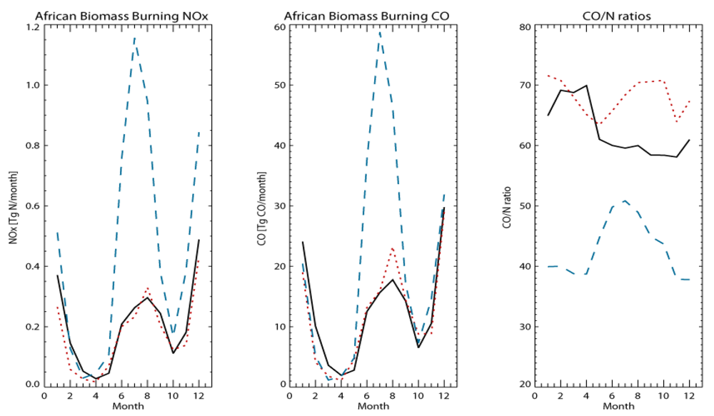
Figure 1 shows differences in the seasonal cycle of Africa BB emissions for both NOx (left) and CO (middle), along with the corresponding seasonal cycle in the CO/N ratios (right). The two seasonal peaks in BB emissions occur from November to January (NDJ) in the Northern Hemisphere (NH) and from June to September (JJAS) in the SH. Largest differences occur between GFEDv2 and AMMABB during boreal summertime and are associated with the intense burning which occurs in southern Africa during this season. For NOx, differences of ~50% also occur from NH burning during boreal wintertime. For both of the GFED inventories there are larger monthly emissions from NH burning than SH burning, whereas for AMMABB the emissions from SH burning dominate. Comparing GFEDv3 and AMMABB shows that the CO BB emission fluxes become quite similar from January to April compared to the corresponding NOx emissions. Given that the emission factors for each trace species are similar between inventories this difference is related to the cumulative effect of differences in the burned area product, vegetation classifications and land use maps. The seasonal variation in the CO/N ratio shows that although the magnitude of the monthly CO/N ratios differ by ~30–50%, the seasonal variation becomes more similar between the GFEDv3 and the AMMABB inventories, although for the AMMABB inventory there is a maxima during August.
Figure 1. Comparison of the monthly African (34°S–36°N, 20°W–40°E) emission totals for (left) NOx and (middle) CO in Tg N/month and Tg CO/month, respectively. The seasonal variation in the corresponding CO/N ratio is also shown (right). The inventories are: (__) GFEDv2, (.…) GFEDv3 and (---) AMMABB.
Atmosphere 03 00132 g001
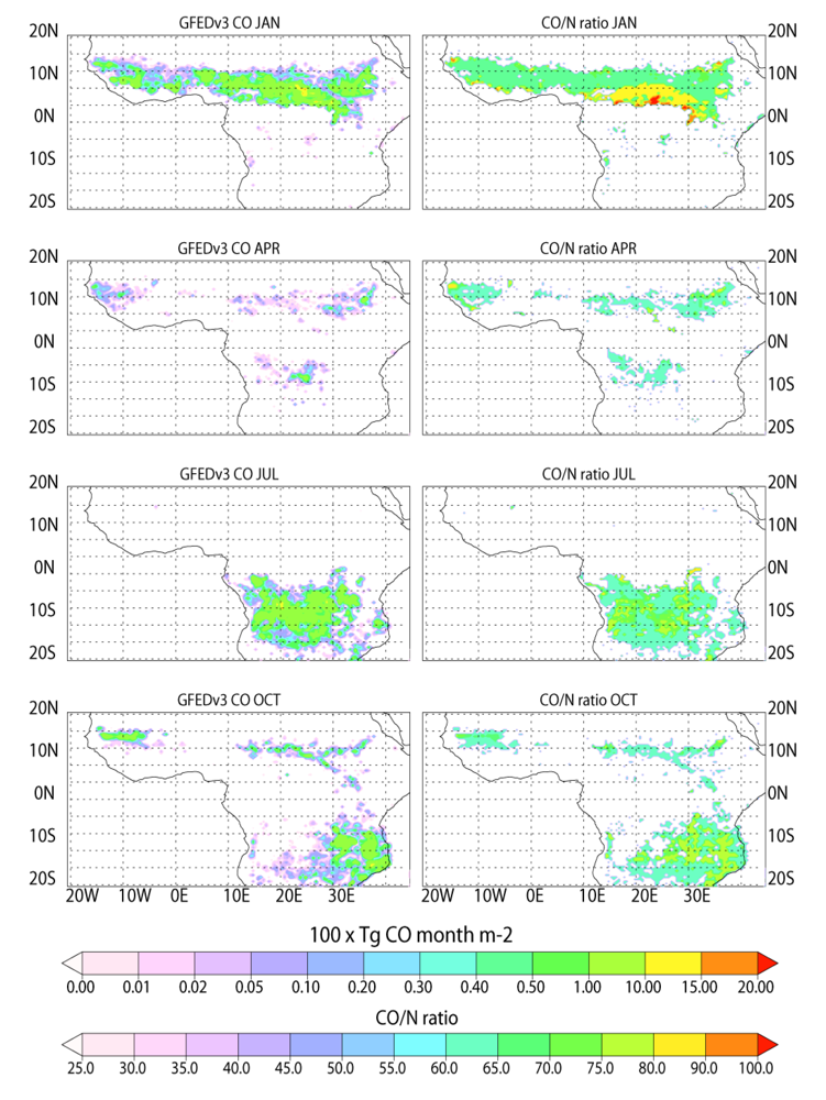
To highlight the differences in the temporal distribution of the emission estimates provided in each inventory, Figure 2 and Figure 3 show the monthly BB emission estimates for CO from Africa for January, April, July and October 2006 as provided in the GFEDv3 and AMMABB emission inventories, respectively. The corresponding CO/N ratios are also shown in all instances. Each emission inventory is shown on a 0.5° × 0.5° resolution. Both figures also show that there is significant variability with respect to the intensity of fires across any given latitude range for any given month. Comparing the total burned area in Africa for 2006 gives 195 × 104 km2 for the L3JRC product [42] and 237 × 104 km2 for the GFEDv3 product [32]. This results in the burned area in the L3JRC product being approximately half as large in northern Africa and two-thirds as large in southern Africa [32]. Therefore, the amount of emissions released per unit area burnt is larger in the AMMABB inventory.
Figure 2. The temporal distribution in African BB for (top to bottom) January, April, July and October during 2006 as provided in the GFEDv3 emission inventory. The corresponding CO/N ratio is also provided for all months.
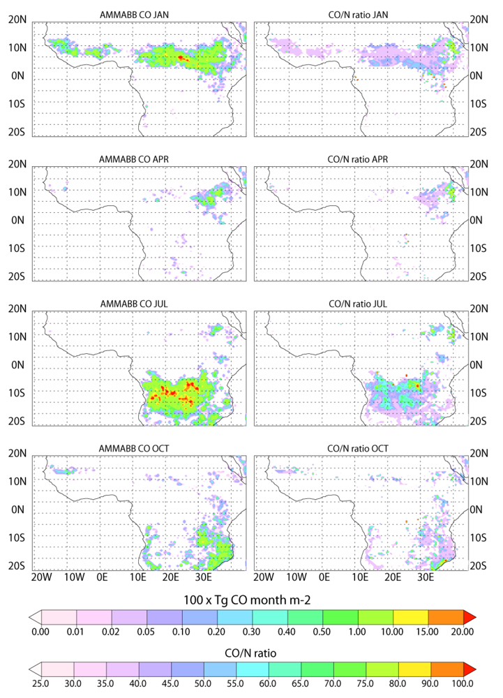
Atmosphere 03 00132 g002
Figure 3. As for Figure 2 except showing the temporal distribution of the AMMABB emission inventory.
Atmosphere 03 00132 g002
In general the seasonal hemispheric distribution is similar, although the extent of burning below (above) the equator is larger in the AMMABB inventory for January (July). The longitudinal distribution in the burning pattern is also very different, where the GFEDv3 inventory has more burning in West Africa throughout the year. Conversely the AMMABB inventory displays more burning activity towards the Horn of Africa. Previous studies have concluded that there is an underestimation in BB in Western Africa in the AMMABB inventory as a result of the L3JRC burned area product [10,40]. Stroppiana et al. [10] have performed direct comparisons of BB CO emissions derived for Africa during 2003 between the GFEDv3 and AMMABB inventories and found a correlation co-efficient (R2) of 0.47, which agrees better than for other regions such as e.g., North America, where the reliability of the L3JRC burnt area product is thought to be low [42]. They have also shown that for the three main land cover types (forest, savanna/grassland and agriculture) there are significant differences in the contribution of CO from each land type in Africa.
For much of the burning region the GFEDv3 inventory has CO/N ratios that range between 60 and 70, although there are regions in southern Africa which ratios can be as high as 80. The corresponding ratios in the AMMABB inventory are typically lower around 35 to 50, although the more intense burning events have ratios which are higher around 70 to 90. When applied in TM4, the spatial variability in these CO/N ratios becomes somewhat homogenized due to the coarsening step onto the horizontal grid of 3° × 2°. Thus using a model with higher resolution would introduce more significant regional variability into the African domain with respect to the CO/N ratio compared to the simulations presented here, which would subsequently affect tropospheric O3 production [43].
Finally we investigate the differences between the GFEDv2 and GFEDv2 8-day emission inventories for African (34°S–34°N, 20°W–40°E) CO emissions. Even if the annually integrated emission totals are approximately equal between the two different GFEDv2 inventories, the segregation of the emission fluxes into 8-day composites may result in different totals when the resulting emission is summed per calendar month. 
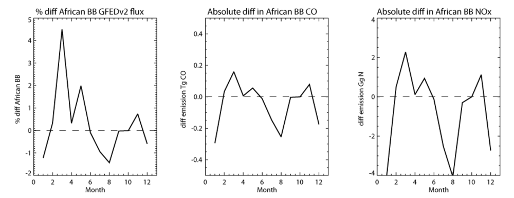
Figure 4 shows the percentage differences in the monthly BB emissions fluxes from the African domain for 2006, as given in the 1° × 1° emission inventories used in this study. Also shown are the absolute differences in Tg CO and Gg N per month. It can be seen that there are generally decreases during the intensive BB seasons NDJ and JJAS. Integrating the absolute difference for the entire year results in a decrease of 0.5 Tg CO yr−1 and 8.9 Gg N yr−1 when applying the GFEDv2 8-day emission inventory for the African domain. These differences shift in location as governed by the location of the seasonal BB activity.
Figure 4. The percentage difference in the monthly BB emission fluxes from Africa (34°S–34°N, 20°W–40°E) between the GFEDv2 and GFEDv2 8-day emission inventories. Also shown is the absolute difference in Tg CO and Gg N per month. The differences are calculated as (8-DAY-MONTHLY)/MONTHLY × 100.
Atmosphere 03 00132 g004

4. The Impact on the Composition of the Southern Hemisphere

4.1. Surface Air Quality; Influence of BB Inventory

Local air quality in the SH has been shown to be sensitive to African BB, with simulated effects occurring thousands of kilometers away in Central America towards the west and Oceania towards the east [4,44]. Here we investigate the sensitivity of near-surface air quality towards the uncertainty in the bottom-up BB emission estimates provided for 2006, where the different CO/N ratios and flux estimates introduce variations in the chemical processing of polluted air-masses, and thus the long range transport of emissions out of Africa. Figure 5 shows the seasonal differences in CO, O3, NOx, and OH in the lowest few kilometers of the troposphere for December-January-February (DJF) and June-July-August (JJA) when comparing simulations using the GFEDv3 and AMMABB emission inventories. This represents the maximal differences between the chosen BB inventories listed in Table 3, and therefore will introduce the largest differences between simulations.
In general it can be seen that the variability introduced by the uncertainty associated with SH BB is significantly larger than the uncertainty associated with NH BB, where the magnitude of the differences in African BB emissions are largest for JJAS (see Figure 1). Interestingly there are also decreases in near-surface CO and NOx around the West African coast related to the differences in the distribution of the regional fire activity between the BB emission inventories. Previous comparisons between inventories have shown that the AMMABB inventory underestimates BB emissions from Western Africa compared to other BB emission inventories [10]. The seasonal differences in the burning activity introduce a strong signature in the impact on near-surface air quality in the SH. For DJF the effect in the SH is limited due to the southerly transport of BB plumes from burning events in northern Africa being limited to the westerly outflow regions as a result of the blocking which occurs due to the location of the Intertropical Convergence Zone (ITCZ). This is in contrast to JJA, where the most intense burning shifts towards the south enhancing the impact occur on SH air quality (~5–10% for CO). For tropospheric O3 maximal impact occurs in and around the African continent as would be expected considering the differences in the atmospheric lifetimes between both trace species. The differences in the SH are principally caused by increases in the in situ chemical production, which occurs away from the African BB source regions. This is due to the corresponding increases in the long range transport of NOx as peroxy-acetyl nitrate (PAN) (not shown). Once PAN is lofted into the FT the low temperatures result in an atmospheric lifetime of tens of days, allowing transport out of the main source regions. Upon decomposition PAN acts as an important chemical reservoir for introducing reactive nitrogen into remote regions [45]. The associated impact on OH is limited to near the source regions, as governed by the increases in tropospheric O3.
When performing a similar comparison between the GFEDv2 and GFEDv3 simulations (not shown), the differences in the monthly emission fluxes between the two emission inventories shown in Figure 1 introduce a seasonal dependency in the absolute differences in the resident concentrations near the surface in and around Africa. There is some degree of temporal variability introduced between both emission inventories, which is somewhat dependant on the particular trace species. For instance, for DJF the GFEDv3 emission inventory estimates a higher emission flux for CO around Nigeria and a lower (higher) emission flux for NOx in the NH BB regions towards the east (north) of Africa. For the westerly outflow there are generally increases during DJF and decreases during JJA, where maximal differences are of the order of ~10%. For the background there are generally decreases (increases) in CO (O3) of a few percent. Thus, the main differences are limited to the tropics (30°S–30°N).
Figure 5. The relative percentage differences in the global near-surface concentrations for (a) CO; (b) O3; (c) NOx and (d) OH for seasons DJF (left) and JJA (right) between GFEDv3 and AMMABB. The relative differences are calculated as ((AMMABB-GFEDv3)/GFEDv3) × 100.
Atmosphere 03 00132 g005

4.2. Surface Air Quality; Influence of Temporal Distribution and Injection Height

Recent studies have shown that increasing the update frequency of boreal BB emissions in a CTM can make a significant difference to the simulated effects of BB on both local and regional air quality [46]. For African BB similar effects have been shown concerning the transport of pollutants in the westerly outflow during JJA [3]. Here we investigate the effect of applying the GFEDv2 8-day emission inventory on near-surface air quality both near the source regions and at global scale. It should be noted that the GFEDv2 8-day inventory is applied for all continents in this instance and not limited to Africa as in some of the other sensitivity studies. For brevity, we limit the discussion to those changes which occur in the tropics and SH.
Figure 6 shows the seasonal differences in near-surface CO, O3, NOx, and OH between the GFEDv2 and 8-DAY simulations for DJF and JJA. As would be expected from the comparisons of the various BB emission inventories made in Figure 1 and Figure 4, the magnitude of the differences between simulations adopting the different GFEDv2 inventories are considerably smaller than the differences shown between the alternative BB inventories (Figure 5). The variation in integrated monthly emission fluxes between the GFEDv2 monthly and 8-day inventories (Figure 4) imposes a seasonality regarding the effects of increasing the update frequency of the temporal distribution, with the influence during JJA being much larger than during DJF as a result of differences in the seasonally integrated BB emission fluxes. Near regions exhibiting high burning activity (e.g., South America and southern Africa) decreases in CO and O3 of between ~5 and 10% occur for the near-surface, showing that the differences in the monthly emission totals are important over the continents. Seasonal differences also occur in near-surface CO and O3 at higher latitudes >60°N/S, although are limited to ±2% due to the much lower regional BB emission fluxes (not shown). Although there is a qualitative agreement in the regional effects around the northern US between our study and that of Chen et al. [46], the impacts in our simulations are much smaller most likely related to the differences in the prescribed injection heights (where BB emissions are introduced below 800 hPa in Chen et al. [46] compared to below 500 hPa in our simulations). Recent studies have shown that boreal BB emissions are typically lofted well above the boundary layer [47], which supports the recommendations for latitudinally dependant injection height adopted here [11].
Similar comparisons calculated between the GFEDv2 and HIGH-IH simulation (not shown) reveal that the corresponding differences near the tropical BB source regions generally lead to increases of up to 3% regardless of season. Thus, the regional effect around the BB source regions is the opposite of that shown in Figure 6. In both simulations the majority of the daily BB emissions are introduced into the boundary layer due to the application of the daily burning cycle. It should be noted that the updated injection heights are only applied for the latitude range 30°S–30°N. Previous modeling studies have shown that, for the boreal regions, BB emissions can be injected directly above the boundary layer, reaching the upper troposphere in some instances [48,49] and affecting regional air quality. For tropical BB the effects are more limited as they do not enter the FT.
Figure 6. The relative percentage differences in the global near-surface concentrations for (a) CO; (b) O3; (c) NOx; and (d) OH for seasons DJF (left) and JJA (right) between GFEDv2 and 8-DAY. The relative differences are calculated as (8-DAY-GFEDv2)/GFEDv2) × 100.
Atmosphere 03 00132 g006
In summary, comparing the distribution of pollutants at the near-surface in the tropics shows that increasing the temporal distribution of BB burning events has a larger, but opposite, effect than increasing the injection height at which the emissions are introduced. This agrees with the findings of previous studies [3,46] although the lack of measurement datasets for near-surface air quality in the tropics means that it is difficult to determine which sensitivity test results in the optimal model performance. However, for the outflow regions, we make comparisons in the following section. Implementing both updates simultaneously would result in some degree of cancellation of effects around the burning regions.

4.3. Comparison against Observations

The distribution of CO and O3 simulated by TM4 in and around Africa has already been assessed in the literature for JJA as compared against a host of different in situ measurement datasets [3,28]. For instance, a recent multi-model study involving TM4 focused on comparisons of CO in the UT above Africa during August 2006 [29]. The main source of CO during this month is BB in southern Africa meaning that such comparisons act as a good indication of the performance of TM4 directly above the BB emission sources. Simulations were performed using the AMMABB emission inventory, similar to those described in this paper. Comparisons of CO at 215 hPa against satellite observations from the Microwave Limb Sounder (MLS) [50] have shown that TM4 can capture the latitudinal distribution quite well over southern Africa and in the outflow towards the west. When comparing against in situ observations of CO made in the African UT as part of the MOZAIC in-flight measurement program [51], TM4 shows a maximum at 250 hPa which is located too far north by 6° and overestimates resident mixing ratios at the maximum by ~20 ppb. Similar comparisons made against TM4 simulations using the GFEDv2 emission inventory generally underpredict the MOZAIC measurements between 20°S and 20°N. Therefore neither emission inventory can be considered to be optimal in capturing the measured concentrations of CO into the UT. The transport out of the region is sensitive to the accuracy of the Tietdke convective parameterization [52] employed in TM4 for the description of convective mixing out of the boundary layer. Barret et al. [29] have shown that the Tietdke scheme results in weaker convective mixing than other alternative parameterizations integrated into other CTMs [29]. This has implications regarding the efficiency of long-range transport of trace gases towards the west during JJA as presented here.
In this study we build on these previous studies and examine if TM4 can capture the observed seasonal cycle and the variability in surface mixing ratios in the tropics and SH. For this purpose we make comparisons of co-located model output with ground based flask measurements taken as part of the NOAA ESRL global network [53,54]. Figure 7 shows comparisons of monthly mean mixing ratios from the NONE, GFEDv3 and AMMABB simulations against the corresponding measurements for selected locations in the SH.
The model monthly mean values are calculated using only days where observations were available in order to make a valid comparison.
Figure 7. The seasonal cycle of surface CO in Africa and the Southern Hemisphere. The NOAA ESRL measurements stations shown are (Top row) Assekram (23.1°N, 5.3°E), Ascension Island (7.9°S, 14.4°W), Crozet Island (46.3°S, 51.5°E); (Middle row) Seychelles (4.7°S, 55.2°E), Easter Island (27.2°S, 109.5°W), American Samoa (14.3°S, 170.6°W); (Bottom row) Christmas Island (1.4°N, 157.1°W), Tierra del Fuego (54.9°S, 68.5°W) and Syowa Antarctica (69.0°S, 39.6°E). The simulations shown are NONE (black), GFEDv3 (red) and AMMABB (blue).
Atmosphere 03 00132 g007
For certain months the 1-σ deviation of the mean in the observations is much larger than that calculated for the model monthly means (not shown), e.g., at site EIC. This shows that the daily variability seen in the observations is not fully captured by TM4. Potential reasons include the use of monthly emission fluxes and the inadequacies of the ECMWF meteorological dataset in remote regions in the tropics [3]. The only station situated in northern Africa is Asskeram (ASK) in southern Algeria. Here the influence of BB emissions from the SH are negligible, again due to blocking of northerly transport by the ITCZ. For stations directly in the outflow (Ascension Island (ASC) to the west and Crozet Island (CRZ) to the east) and towards high southern latitudes (Tierra Del Fuego (TDF) and Syowa (SYO)) there is a significant difference between the various simulations during JJAS. For these months the AMMABB simulation tends to overestimate surface CO in the outflow by ~20–30%. For the GFEDv3 emission inventory the model captures both the magnitude and phase of the observed seasonal cycles quite well, albeit underestimating during certain months. It is interesting to note that the impact of CO from SH BB can be seen at locations far to the east as American Samoa (SMO), where transport over similar distances has been detected in the FT by the MOPITT instrument [4]. For the other simulations the only discernible difference in the monthly mean mixing ratios calculated using the GFEDv2 and GFEDv3 inventories is that GFEDv3 has a marginally higher value at ASC during August (resulting in a small overestimation).
Figure 8 shows the residual calculated between the model monthly mean mixing ratios and ground based observations for the GFEDv2 and 8-DAY simulations at six of the surface stations included in Figure 7. Focusing on selected stations situated in the easterly and westerly outflow regions and at high southern latitudes shows that although the differences are quite small the impact of temporal variability in tropical BB emissions can be seen over large distances. Comparing values it becomes clear that there is generally a better agreement for the 8-DAY run, which has residual values closer to unity during JJAS at most of the stations. That the measurements sites are located in the SH means there is limited impact of West African BB emissions on the comparisons (Figure 5). A similar comparison for the HIGH-IH run (not shown) reveals minimal differences compared with the GFEDv2 simulation. This provides further evidence that the effect of updating the frequency of the temporal distribution is more important than the relatively small variability in the injection heights of tropical BB. Thus, these comparisons show that BB inventories with high temporal variability (i.e., weekly update frequencies) should be used in preference to those which aggregate burning emissions over an entire month whenever available.
Figure 8. Residual values between the monthly mean CO mixing ratios at the surface for the GFEDv2 and 8-DAY simulations. The residuals are calculated by dividing the model monthly means by the observational monthly means at selected stations from the NOAA ESRL network. The measurements stations shown are (top row) Seychelles (4.7°S, 55.2°E), Crozet Island (46.3°S, 51.5°E); (middle row) Ascension Island (7.9°S, 14.4°W), Tierra del Fuego(54.9°S, 68.5°W) and (bottom row) Palmer (64.5°S, 0.4°W) and Syowa Antarctica (69.0°S, 39.6°E). The simulations shown are GFEDv2 (blue) and 8-DAY (red).
Atmosphere 03 00132 g008

4.4. Long Range Transport from Africa; Influence of BB Inventory

To quantify the variability in long range transport out of Africa, Figure 9 shows the seasonal differences in CO, O3, NOx, and OH between the GFEDv3 and AMMABB simulations in the middle troposphere at ~550 hPa. Again the differences are maximal for season JJA, where significantly more CO and NOx is exported outside the tropics into the SH for the AMMABB simulation, resulting in increases of ~50–70% in the resident mixing ratios in the FT. The maximal differences occur directly over the burning regions due to strong convective uplift out of the boundary layer, and also along the westerly and easterly outflow pathways. Even though the photo-chemical production efficiency of OH increases by ~7% during JJA there is a net decrease in the seasonal mixing ratio in the tropical FT of around ~5%. This is due to the enhanced scavenging by the additional CO which is lifted out of the boundary layer in the AMMABB simulation, where CO is a dominant chemical sink term for OH under low NOx conditions [55]. Thus the composition of the FT in the SH is rather sensitive to the BB emission inventory applied for Africa. The perturbations seen above Oceania also agree with observational evidence published in the literature [4]. It should be noted that convective parameterization in TM4 has been shown to be rather weak over Africa [29] meaning that the effects shown here could be smaller than those captured by other CTMs. We discuss the implications for the variation in the oxidative capacity of the SH in [Section 5].
In a previous study the distribution of O3 in the UT simulated by TM4 has been shown to compare favorably against MOZAIC observations at ~250 hPa for August 2006 when using the AMMABB BB emission inventory [29], although the minimum observed between 5°S–5°N is over-estimated by ~5–10 ppb. Similar comparisons for simulations using the GFEDv2 BB emission inventory generally lead to an under prediction in the SH of ~10–20 ppb. To investigate the agreement at locations further away from the source regions we perform additional comparisons against measurements. Figure 10 shows comparisons of seasonal ozonesonde composites for DJF and JJA at the tropical stations Paramaribo (5.8°N, 55.2°W), to the west, and La Reunion (21.1°S, 55.5°E), to the east. Co-located model composites are also shown for NONE, GFEDv3 and AMMABB. Both of these stations are located in the outflow regions where the seasonal variability in tropospheric O3 between the chosen BB emission inventories is of the order of ~5–15% (Figure 9). The influence of African BB on tropospheric O3 away from the source regions is highly dependent on the chemical mechanism employed to describe the chemical evolution in the polluted plumes during transport, which typically take days to reach the location of the measurement sites [56]. For stations further south (e.g., Neumayer (70.7°S, 8.3°W)) the effects are limited to a few percent and, for brevity, are not shown. The non-linearity associated with tropospheric O3 formation near high emission sources of NOx and NMHC [57] means that the observed differences in O3 in the outflow are not directly scalable to the differences in BB NOx between inventories.
Figure 9. The relative percentage differences in the global concentrations for (a) CO; (b) O3; (c) NOx; and (d) OH between the GFEDv3 and AMMABB simulations for seasons DJF (left) and JJA (right) in the middle troposphere of the atmosphere at ~550 hPa. The difference is calculated as (AMMABB-GFEDv3)/GFEDv3.
Atmosphere 03 00132 g009
Figure 10. Seasonal comparisons of co-located tropospheric ozone profile composites for seasons DJF (Top) and JJA (Bottom). The soundings stations shown are (Left) Paramaribo (5.8°N, 55.2°W) and (Right) La Reunion Island (21.1°S, 55.5°E), with the measurements taken from the SHADOZ database. The black line represents the measurements along with the 1-σ deviation of the seasonal means, with the number of observations used being shown in the top left of each panel. Three simulations are shown: NONE (blue), GFEDv3 (red) and AMMABB (green).
Atmosphere 03 00132 g010
For Paramaribo African BB influences the lower and middle troposphere during both seasons to the same degree. Even in the absence of African BB the model over predicts the near-surface O3 as a result of TM4 either having a low dry deposition flux over forested regions [58] or an over estimation of local emission sources, which affect mixing ratios in the boundary layer near the measurement site [59]. A further complication is that the measurement site is near the coast, where the diurnal cycle of atmospheric mixing that occurs near the land-sea boundary is difficult to capture in a global model using a rather coarse horizontal resolution. Comparing simulations which include African BB shows that there is a ~15–20% influence at the eastern coast of South America. Even though the emissions are lofted rapidly into the FT the simulations show effects throughout the tropospheric column. In Africa it has also been shown that the description of transport across the ITCZ by ECMWF operational meteorology is significantly influenced by the frequency of the measurements which are assimilated into the forecasting system [3]. For JJA this leads to an over-estimation of the influence of BB from southern Africa on the lower troposphere over the West African coast for this year in TM4. A similar effect seems to be visible at Paramaribo, where the magnitude of the effects is homogenous from the surface to 250 hPa, again suggesting too efficient transport of air influenced by African BB into the lower troposphere. Although the AMMABB simulation shows that highest mixing ratios the quality of the agreement is worse (better) in the LT (FT). Therefore it is difficult to use this comparison for placing emphasis on the quality of each BB inventory due to other biases that seem to exist in TM4.
For La Reunion the comparisons show a somewhat different behavior. The location of the measurement site, meteorological variability and seasonality with respect to the location of African BB in the SH limits the influence of African BB to JJA only. The largest effects occur in the upper troposphere between 300–500 hPa. The measurement site is located on a small island and can therefore be seen as representative of the marine boundary layer in the tropical SH. Being situated away from strong emission sources, the gradient of the tropospheric O3 profile is captured relatively well. Comparing simulations shows that the AMMABB emission inventory results in the best comparison of all those shown, where the contribution from Africa BB is ~13% to the simulated O3 profile. The differences in the boundary layer are rather minimal showing that the ECMWF meteorology does not transport too much.
Comparing the GFEDv2 and GFEDv3 simulations (not shown) similar to Figure 9 reveals that differences in the resident mixing ratios of CO and O3 in the FT of between ~±2 and 10%, with the maximal differences again being found directly above the main BB source regions and in the outflow. The differences in the background are limited to a few percent. As for the near-surface, there is strong seasonality in the simulated differences with decreases (increases) during DJF (JJA) as governed by the seasonality in African BB.

4.5. Long Range Transport from Africa; Influence of Temporal Distribution and Injection Height

Figure 11 shows the seasonal differences in long range transport at ~550 hPa when comparing the GFEDv2 and 8-day simulations, similar to that shown in Figure 9. Again, the differences are small (~2–5%) compared to the differences shown between the AMMABB and GFEDv3 BB emission inventories and there is a pronounced seasonality in the effects. There is also a latitudinal dependency in the perturbations related to the respective increases and decreases in the monthly aggregated BB emissions of CO and NOx between the two simulations for various regions (not shown). For DJF the differences are limited to the order of ±2% for tropospheric CO and O3, where a strong signature for CO is seen in and around Indonesia. For JJA the largest impact is in the SH, related to burning in South America, southern Africa and Indonesia. The largest differences occur for NOx, where the amount transported away from the source regions decreases due to less PAN being transported into the region (not shown). One interesting feature is the decrease in the mixing ratio of OH in spite of a corresponding decrease in the mixing ratio of CO. Analyzing the chemical budget terms shows that the there is enhanced loss of OH via the oxidation of O3, methyl peroxide (CH3OOH), CH4 and H2 in the 8-day run, which compensates for the reduced scavenging of OH by CO.
Finally, similar comparisons made between the GFEDv2 and HIGH-IH simulation (not shown) reveal that increases of a few percent occur directly above the most active burning regions due to venting from the boundary layer but effects in the outflow are rather negligible. This finding supports the conclusion drawn in Section 4.2, i.e., that increasing the temporal distribution of tropical BB emissions has a more pronounced effect on tropical and SH tropospheric composition than increasing the injection height.
Figure 11. The relative percentage differences in the global concentrations for (a) CO; (b) O3; (c) NOx; and (d) OH between the GFEDv2 and 8-DAY simulations for seasons DJF (left) and JJA (right) in the middle troposphere of the atmosphere at ~550 hPa. The difference is calculated as (8-DAY-GFEDv2)/GFEDv2.
Atmosphere 03 00132 g011

5. Changes to Global Burdens and Tropospheric Lifetimes

The large variability in the estimates of trace gas emissions contained in the different bottom-up BB emission inventories for Africa shown in Table 2 has the potential to significantly impact the burdens and lifetimes of the ubiquitous trace gas species, O3, CO and CH4. In order to investigate the perturbations introduced we use a set of diagnostics which have been defined for assessing the performance of CTMs during multi-model intercomparison studies [16]. For brevity we limit the discussion to the changes introduced by the different BB emission estimates, with the differences due to temporal variability and injection height being rather small in comparison and therefore of lesser interest.
For tropospheric O3 the variability in the burden (BO3), tropospheric lifetime (τO3) and net annual production terms (pO3) are given in Table 4 for the different BB emission inventories. The percentage differences that are given are calculated with respect to the NONE simulation. Here we define a climatological tropopause [60] throughout the analysis which ensures that the mass of the troposphere remains constant for all simulations therefore allowing a valid comparison of tropospheric burdens and lifetimes.
Table 4. The variability in the global tropospheric burden and lifetime of O3 during 2006 when adopting the different BB emission inventories for Africa. Also shown is the total global in situ chemical production of O3. The climatological tropopause of Lawrence et al. [60] is used to define the troposphere throughout. The relative percentage changes of tropospheric lifetimes and global burdens as compared to the NONE simulation are given in parenthesis.
BO3 (Tg O3)O3 Lifetime (days)pO3 (Tg O3)
NONE317.724.14328.1
GFEDv2323.0 (+1.7)23.6 (−1.9)4500.3 (+4.0)
GFEDv3323.2 (+1.8)23.7 (−1.6)4492.5 (+3.8)
AMMABB332.2 (+4.6)23.3 (−3.0)4641.8 (+7.2)
AMMABB_LOWNOX325.7 (+2.5)23.6 (−1.9)4555.2 (+5.2)
The introduction of African BB (as defined in the GFEDv2, GFEDv3 and AMMABB simulations) increases BO3 between 1.7 and 4.6%, resulting in a mean BO3 of 326.1 ± 5.3 Tg O3 (with an associated uncertainty of ~1.6%). The corresponding change in τO3 is from −1.9% to −3.0%, resulting in a mean τO3 of 23.5 ± 0.2 days (with an associated uncertainty of ~0.9%). The corresponding differences in BCO, τCO, and τCH4 are given in Table 5, along with the total mass of CH4 that is oxidized in each simulation. For CH4 the total mass that is oxidized is equal to the amount oxidized by OH, with a fixed soil sink of 30 Tg yr−1 and a stratospheric sink of 40 Tg yr−1, as outlined in Stevenson et al. [16]. Comparing values reveals that African BB decreases the global lifetimes of both trace gases across the range of CO/N ratios contained in the different BB inventories (~43–69), i.e., regardless of the seasonal CO emission flux. This gives mean atmospheric lifetimes across all three BB inventories of τCO = 53.4 ± 0.4 days and τCH4 = 8.70 ± 0.02 years, which translates to an uncertainty of ~0.7% and ~0.2%, respectively.
Table 5. The global tropospheric burdens and lifetimes of CO, and CH4 for the different BB emission inventories adopted for Africa during 2006.
BCO (Tg CO)CO Lifetime (days)Mass CH4 OxidisedCH4 Lifetime (years)
NONE302.654.4499.48.75
GFEDv2320.8 (+6.0)53.6 (+1.5)501.8 (+0.5)8.72 (−0.4)
GFEDv3321.2 (+6.1)53.6 (+1.5)502.1 (+0.5)8.71 (−0.5)
AMMABB332.2 (+9.9)52.9 (+2.8)504.3 (+1.0)8.68 (−0.8)
AMMABB_LOWNOX339.1 (+12.0)54.3 (+0.2)495.1 (-0.9)8.82 (+0.8)
Increasing NOx emissions cause an associated increase in pO3, although a moderating constraint on the variability in both pO3 and BO3 is the enhanced loss of reactive nitrogen via wet deposition as nitric acid (~1 Tg N yr−1extra when adopting the AMMA BB inventory). Thus the oxidative capacity of the global troposphere is enhanced as a result of African BB.
The uncertainty associated with the mean τCH4 is significant due to the relatively modest increases which occur in the yearly growth rate of fractions of a percent [20], where the variability in the mass of CH4 oxidized across all simulations translates to a variability of °0.25 ppbv yr−1 in the growth rate. The reduction in τCH4 is largest for AMMABB which may be counterintuitive because it also exhibits the highest CO emissions (cf. Table 2). From the CO consumption argument [21] one would expect an increase in τCH4 due to the increased scavenging of OH by CO in the tropics, where the majority of CH4 is oxidized. The AMMABB_LOWNOX simulation shows that increases in τCH4 are only observed if the CO/N ratio is relatively high (~90), which reduces the chemical production of ozone as shown in Table 4. Such high CO/N ratios are typically associated with peat burning, charcoal production or animal waste burning [
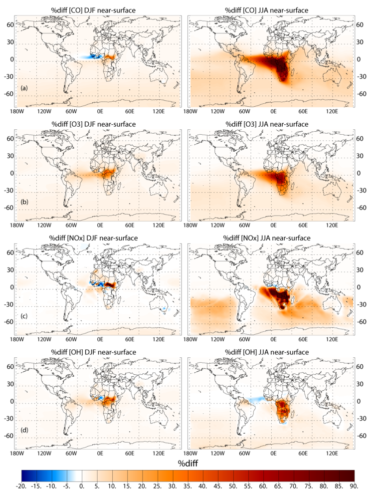
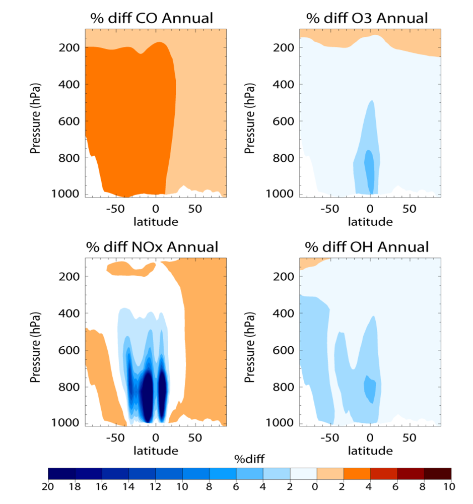
6] and thus should be considered an upper limit in terms of realistic CO/N ratios. To show the sensitivity of global tropospheric composition to the CO/N ratio the annual zonal mean differences between the AMMABB and AMMABB_LOWNOX simulations are shown in Figure 12. That there is a simultaneous increase in CO and decrease in OH under low NOx conditions indicates that there is less oxidation capacity in the troposphere for the oxidation of CH4 resulting in a subsequent increase in its atmospheric lifetime.
Therefore, some mitigation of the effects of high CO emissions from BB occurs due to the associated increase in NOx (and thus O3 and OH). It cannot be expected that the high CO/N ratios defined in the AMMABB_LOWNOX simulation would occur on a continental scale therefore it is likely that increases in τCH4 occur regardless of the inter-annual variability in BB emissions that originate from Africa. It should be noted that the feedback on photolysis rates due to smoke and aerosol particles is not accounted for in these simulations, but are expected to decrease the photo-chemical production of tropospheric O3 in the lower troposphere, thus allowing more CO to be transported out of the region.
Figure 12. The relative percentage differences in the zonal annual mean concentrations for (a) CO; (b) O3; (c) NOx; and (d) OH between the AMMABB and AMMABB_LOWNOX simulations. The differences are calculated as (AMMABB_LOWNOX-AMMABB)/AMMABB ×100.
Atmosphere 03 00132 g012
For Africa, most burning is associated with either savannah and grasslands or woodlands, whose estimated CO/N ratios are 28.8 and 37.0, respectively [6]. The ratios given in Table 3 can be considered aggregates across a wide variety of different vegetation types for the African region, as shown by the regional variability in CO/N ratios shown in Figure 3 and Figure 4. Recently van Leeuwen and van der Werf [61] have shown that when accounting for environmental variables such as precipitation and temperature, CO emissions could be higher for savanna and grasslands per Kg biomass burned significantly impacting emission ratios, although measurements during peak burning periods are necessary to constrain values. In this study we have shown that the global effect of such enhancements would be to increase BCO and BO3 by a few percent, whilst decreasing the atmospheric lifetimes of long-lived trace species.

6. Conclusions

In this study we have investigated the sensitivity of atmospheric composition in the tropics and Southern Hemisphere towards the biomass burning emission inventory adopted for African biomass burning (namely the GFEDv2, GFEDv3 and AMMABB inventories). Comparing the monthly emission totals for the African continent between the different biomass burning inventories for 2006 shows that the intensity, location and associated CO/N ratios of large scale biomass burning events vary significantly, although the seasonality between inventories is rather similar. For the most active burning season of June-July-August-September this leads to differences of >100% in the monthly emission fluxes from Africa. When comparing the GFEDv2 monthly and 8-day emission inventories the integrated monthly emission estimates vary by ±2 Gg and ±0.2 Tg for nitrogen oxides and carbon monoxide (CO), respectively. These differences are introduced as a result of increasing the temporal resolution of the burning events, although the annual emission flux remains approximately equal. The spatial distribution of burning events within Africa is also highly variable when comparing different inventories, especially for the north of the Equator during the boreal winter.
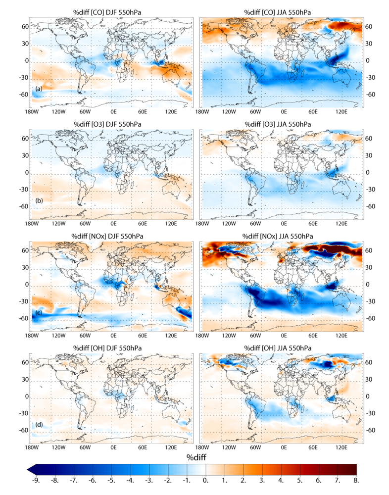
Applying the different biomass burning emission inventories in a 3D global chemistry-transport model leads to significant differences in the near-surface ozone (O3) and CO, especially during June-July-August in the Southern Hemisphere (SH). When comparing the simulations which adopt the GFEDv3 and AMMABB emission inventories, differences in near-surface O3 and CO of ~50–90% occur during June-July-August near the source regions. In the remote SH differences are of the order of ~5–15%. Increasing the update frequency of the temporal distribution of the burning events from monthly to every 8 days shows decreases of between ~0 and 10% for near-surface O3 and CO near the source regions during both seasons. More modest changes of a few percent occur for the outflow regions. This occurs due to both the changes in the geographic variability of the most intense fires and small differences in the total monthly emission fluxes as defined between inventories. Increasing the injection heights at which trace gas emission from fires are introduced in the tropics (30°S–30°N) results in differences of a few percent limited to regions which exhibit the most intense fires, as found in the literature.
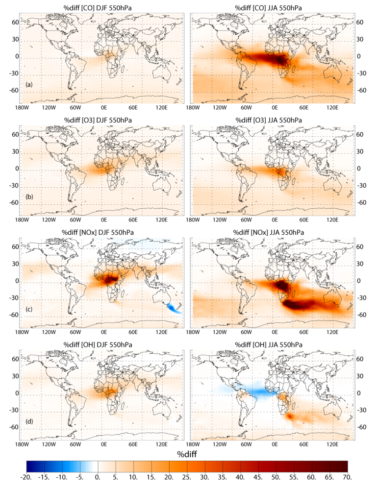
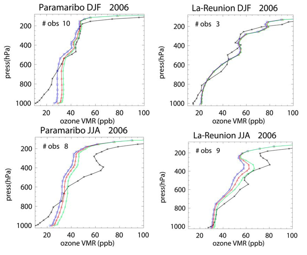
For the long range transport of gases out of Africa substantial differences of ~50–70% in the resident mixing ratios of CO and NOx are simulated in the outflow regions at ~550 hPa, which has a significant impact of the atmospheric burdens of these trace species in the SH. A comparison of the monthly mean mixing ratios for CO from the simulations against ground-based flask measurements shows that the AMMABB inventory tends to overestimate background concentrations during June-July-August-September, with the GFEDv3 emission inventory showing the best correlation. For tropospheric O3 comparisons with composites of tropical ozone soundings taken at locations to the east of Africa show that the AMMABB emission inventory shows a better agreement for the middle and upper troposphere, although this is also dependant on both the chemical mechanism which is employed, the efficiency of the convective and advective mixing and the accuracy of the meteorological data used to drive the chemistry-transport model.
The influence of Africa biomass burning on the atmospheric burdens of CO and O3 results in increases of between 6.0–12.0% and 1.9–3.0% across inventories, respectively. This introduces an associated uncertainty into the total tropospheric burdens of ~1.6% and ~0.9%, respectively. For the atmospheric lifetimes of CO, O3 and CH4 the values are 53.4 ± 0.4 days, 23.5 ± 0.2 days and 8.70 ± 0.2 years are calculated, respectively, with an associated uncertainty of ~0.9%, ~0.7% and ~0.2%. Decreases in τCH4 occur across all BB inventories regardless of the differences in the total CO emitted from African BB. This is due to the associated differences in the CO/N ratio being rather small between the inventories on the horizontal resolution employed for the study. Thus the increase in the CO emission is partially mitigated by the simultaneous increase in the oxidative capacity around the source regions and, subsequently, in the outflow. Only when the CO/N ratio exceeds ~90 does the increase in the tropospheric CO burden result in decreases in the lifetime of CH4. This has important implications when explaining the relationship between the inter-annual variability in the global CH4 growth rate and the inter-annual variability in BB emissions from Africa.

References

  1. Thompson, A.M.; Witte, J.C.; Oltmans, S.J.; Schmidin, F.J.; Logan, J.A.; Fujiwara, M.; Kirchhoff, V.W.J.H.; Posny, F.; Coetzee, G.J.R.; Hoegger, B.; et al. Southern Hemisphere Additional Ozonesondes (SHADOZ) 1998-2000 tropical ozone climatology: 2. Tropospheric variability and the zonal wave-one. J. Geophys. Res. 2003, 108, 8241. [Google Scholar]
  2. Ziemke, J.R.; Chandra, S; Duncan, B.N.; Schoeberl, M.R.; Torres, O.; Damon, M.R.; Bhartia, P.K. Recent biomass burning in the tropics and related changes in tropospheric ozone. Geophys. Res. Lett. 2009, 36, L15819. [Google Scholar]
  3. Williams, J.E.; Scheele, M.P.; van Velthoven, P.F.J.; Thouret, V.; Saunois, M.; Reeves, C.E.; Cammas, J.-P. The influence of biomass burning and transport on tropospheric composition over the tropical Atlantic Ocean and Equatorial Africa during the West African Monsoon in 2006. Atmos. Phys. Chem. 2010, 10, 9797–9817. [Google Scholar] [CrossRef]
  4. Edwards, D.P.; Emmons, L.K.; Gille, J.C.; Chu, A.; Attié, J.-L.; Wood, S.W.; Haywood, J.; Deeter, M.N.; Massie, S.T.; Ziskin, D.C.; et al. Satellite-observed pollution from Southern Hemisphere biomass burning. J. Geophys. Res. 2006, 111, D14312. [Google Scholar]
  5. Jain, A.K. Global estimation of CO emissions using three sets of satellite data for burned area. Atmos. Environ. 2007, 41. [Google Scholar]
  6. van der Werf, G.R.; Randerson, J.T.; Giglio, L.; Collatz, G.J.; Mu, M.; Kasibhatla, P.S.; Morton, D.C.; DeFries, R.S.; Jin, Y.; van Leeuwen, T.T. Global fire emissions and the contribution of deforestation, savanna, forest, agricultural, and peat fires (1997-2009). Atmos. Chem. Phys. 2010, 10, 11707–11735. [Google Scholar]
  7. Liousse, C.; Andreae, M.O.,; Artaxo, P.; Barbosa, P.; Cachier, H.; Grégoire, J.-M.; Hobbs, P.; Lavoué, D.; Mouillot, F.; Penner, J.; et al. Deriving global quantitative estimates for spatial and temporal distributions of biomass burning emissions. In Emissions of Atmospheric Trace Compounds; Granier, C., Artaxo, P., Reeves, C., Eds.; Kluwer Academic Publishers: Dordrecht, The Netherlands, 2004; p. 544. [Google Scholar]
  8. van der Werf, G.R.; Randerson, J.T.; Giglio, L.; Collatz, G.J.; Kasibhatla, P.S.; Arellano, A.F., Jr. Interannual variability in global biomass burning emissions from 1997 to 2004. Atmos. Chem. Phys. 2006, 6, 3423–3441. [Google Scholar] [CrossRef]
  9. Liousse, C.; Guillaume, B.; Grégoire, J.-M.; Mallet, M.; Galy, C.; Pont, V.; Akpo, A.; Bedou, M.; Castéra, P.; Dungall, L.; et al. Updated African biomass burning emission inventories in the frame of the AMMA-IDAF program, with an evaluation of combustion aerosols. Atmos. Phys. Chem. 2010, 10, 9631–9646. [Google Scholar] [CrossRef] [Green Version]
  10. Stroppiana, D.; Brivio, P.A.; Grégoire, J.-M.; Liousse, C.; Guillaume, B.; Granier, C.; Mieville, A.; Chin, M.; Pétron, G. Comparison of global inventories of CO emissions from biomass burning derived from remotely sensed data. Atmos. Chem. Phys. 2010, 10, 12713–12189. [Google Scholar]
  11. Dentener, F.; Kinne, S.; Bond, T.; Boucher, O.; Cofala, J.; Generoso, S.; Ginoux, P.; Gong, S.; Hoelzemann, J.J.; Ito, A.; et al. Emissions of primary aerosol and precursor gases in the years 2000 and 1750 prescribed data-sets for Aerocom. Atmos. Chem. Phys. 2006, 6, 4321–4344. [Google Scholar] [CrossRef]
  12. val Martin, M.; Logan, J.A.; Kahn, R.A.; Leung, F.-Y.; Nelson, D.L.; Diner, D.J. Smoke injection heights from fires in North America: Analysis of 5 years of satellite observations. Atmos. Chem. Phys. 2010, 10, 1491–1510. [Google Scholar] [CrossRef]
  13. Labonne, M.; Breon, F.-M.; Chavallier, F. Injection height of biomass burning aerosols as seen from a spaceborne lidar. Geophys. Res. Letts. 2007, 34, L11806. [Google Scholar]
  14. Tosca, M.G.; Randerson, J.T.; Zender, C.S.; Nelson, D.L.; Diner, D.J.; Logan, J.A. Dynamics of fire plumes and smoke clouds associated with peat and deforestation fires in Indonesia. J. Geophys. Res. 2011, 111, D08207. [Google Scholar]
  15. Shindell, D.T.; Faluvegi, F.; Stevenson, D.S.; Krol, M.C.; Emmons, L.K.; Lamarque, J.-F.; Pétron, G.; Dentener, F.J.; Ellingsen, K.; Schultz, M.G.; et al. Multimodel ensemble simulations of carbon monoxide: Comparison with observations and projected near-future changes. J. Geophys. Res. 2006, 111, D08301. [Google Scholar]
  16. Stevenson, D.S.; Dentener, F.J.; Schultz, M.G.; Ellingsen, K.; van Noije, T.P.C.; Wild, O.; Zeng, G.; Amann, M.; Atherton, C.S.; Bell, N.; et al. Multimodel ensemble simulations of present-day and near-future tropospheric ozone. J. Geophys. Res. 2006, 111, D08301. [Google Scholar]
  17. Duncan, B.N.; West, J.J.; Yoshida, Y.; Fiore, A.M.; Ziemke, J.R. The influence of European pollution on ozone in the Near East and northern Africa. Atmos. Chem. Phys. 2008, 8, 2267–2283. [Google Scholar]
  18. Flanningan, M.D.; Krawchuk, M.A.; de Groot, W.J.; Wotton, B.M.; Gowman, L.M. Implications of changing climate for global wildland fire. Int. J. Wild. Fire 2009, 18, 483–507. [Google Scholar] [CrossRef]
  19. Duncan, B.N.; Bey, I.; Chin, M.; Mickley, L.J.; Fairlie, T.D.; Martin, R.V.; Matsueda, H. Indonesian wildfires of 1997: Impact on Tropospheric Chemistry. J. Geophys. Res. 2003, 108, 4458. [Google Scholar]
  20. Simpson, I.J.; Rowland, F.S.; Meinardi, S.; Blake, D.R. Influence of biomass burning during recent fluctuations in the slow growth of global tropospheric methane. Geophys. Res. Lett. 2006, 33, L22808. [Google Scholar]
  21. Bousquet, P.; Ciais, P.; Miller, J.B.; Dlugokencky, E.J.; Hauglustaine, D.A.; Prigent, C.; van der werf, G.R.; Peylin, P.; Brunke, E.-G.; Carouge, C.; et al. Contribution of anthropogenic and natural sources to atmospheric methane variability. Nature 2006, 443, 439–443. [Google Scholar]
  22. Karlsdόttir, S.B.; Isaksen, I.S.A. Changing methane lifetime: Possible cause for reduced growth. Geophys. Res. Lett. 2000, 27, 93–96. [Google Scholar] [CrossRef]
  23. Dalsøren, S.B.; Isaksen, I.S.A. CTM study of changes in tropospheric hydroxyl distribution 1990-2001 and its impact on methane. Geophys. Res. Lett. 2006, 33. [Google Scholar]
  24. Houweling, S.; Dentener, F.J.; Lelieveld, J. The impact of non-methane hydrocarbon compounds on tropospheric photochemistry. J. Geophys. Res. 1998, 103, 10673–10696. [Google Scholar]
  25. Williams, J.E.; van Noije, T.P.C. KNMI Scientific Report WR 2008-02. On the Upgrading of the Modified Carbon Bond Mechanism IV for Use in Global Chemistry Transport Models, 2008; KNMI: De Bilt, The Netherlands, 2008; p. 64. Available online: http://www.knmi.nl/bibliotheek/knmipubWR/WR2008-02.pdf (accessed on 7 February 2012).
  26. Landgraf, J; Crutzen, P.J. An efficient method for online calculations of photolysis and heating rates. J. Atmos. Sci. 1998, 55, 863–878. [Google Scholar] [CrossRef]
  27. Krol, M.C.; van Weele, M. Implications of variations in photodissociation rates for global tropopsheric chemistry. Atmos. Environ. 1997, 31, 1257–1273. [Google Scholar] [CrossRef]
  28. Williams, J.E.; Scheele, R.; van Velthoven, P.; Bourar, I.; Law, K.; Josse, B.; Peuch, V.-H.; Yang, X.; Pyle, J.; Thouret, V.; et al. S. Global chemistry simulations in the AMMA Multimodel Intercomparison project. Bull. Am. Meteor. Soc. 2010, 91, 611–624. [Google Scholar] [CrossRef]
  29. Barret, B.; Williams, J.E.; Bouarar, I.; Yang, X.; Josse, B.; Law, K.; Pham, M.; le Flochmoën, E.; Liousse, C.; Peuch, V.-H.; et al. Impcat of West African Monsoon convective transport and lightning NOx production upon the upper tropospheric composition: A multi-model study. Atmos. Chem. Phys. 2010, 10, 5719–5738. [Google Scholar] [CrossRef] [Green Version]
  30. Roberts, G.; Wooster, M.J.; Lagoudakis, E. Annual and diurnal african biomass burning temporal dynamics. Biogeosciences 2009, 6, 849–866. [Google Scholar] [CrossRef]
  31. Giglio, L.; van der Werf, G.R.; Randerson, J.T.; Collatz, G.J.; Kasibhatla, P. Global estimation of burned area using MODIS active fire observations. Atmos. Chem. Phys. 2006, 6, 957–974. [Google Scholar] [CrossRef]
  32. Giglio, L.; Randerson, J.T.; van der Werf, G.R.; Kasibhatla, P.S.; Collatz, G.J.; Morton, D.C.; DeFries, R.S. Assessing variability and long-term trends in burned area by merging multiple satellite fire products. Biogeosciences 2010, 7, 1171–1186. [Google Scholar]
  33. Potter, C.S.; Randerson, J.T.; Field, C.B.; Matson, P.A.; Vitousek, P.M.; Mooney, H.A.; Klooster, S.A. Terrestial ecosystem production—A process model based on global satellite and surface data. Global Biogeochem. Cycles 1993, 7, 811–841. [Google Scholar] [CrossRef]
  34. Friedl, M.A.; McIver, D.K.; Hodges, J.C.F.; Zhang, X.Y.; Muchoney, D.; Strahler, A.H.; Woodcock, C.E.; Gopal, S.; Schneider, A.; Cooper, A.; et al. Global land cover mapping from MODIS: Algorithms and early results. Remote Sens. Environ. 2002, 83, 287–302. [Google Scholar] [CrossRef]
  35. Huffman, G.J.; Adler, R.F.; Morrissey, M.; Bolvin, D.T.; Curtis, S.; Joyce, R.; McGavock, B.; Susskind, J. Global precipitation at one-degree resolution from multi-satellite observations. J. Hydrometeor. 2001, 2, 36–50. [Google Scholar] [CrossRef]
  36. Andreae, M.O.; Merlet, P. Emission of trace gases and aerosols from biomass burning. Global Biogeochem. Cycles 2001, 15, 512–525. [Google Scholar]
  37. Christian, T.J.; Kleiss, B.; Yokelson, R.J.; Holzinger, R.; Crutzen, P.J.; Hao, W.M.; Saharjo, B.H.; Ward, D.E. Comprehensive laboratory measurements of biomass-burning emissions: 1. Emissions from Indonesian, African and other fuels. J. Geophys. Res. 2003, 108, 4719–1. [Google Scholar]
  38. Hooghiemstra, P.; Krol, M.C.; Meirink, J.F.; Bergamaschi, P.; van der Werf, G.R.; Novelli, P.C.; Aben, I.; Röckmann, T. Optimizing global CO emission estimates using a four-dimensional variational data assimilation system and surface network obervations. Atmos. Chem. Phys. 2011, 11, 4705–4723. [Google Scholar]
  39. Pétron, G.; Granier, C.; Khattatov, B.; Yudin, V.; Larmarque, J.-F.; Emmons, L.; Gille, J.; Edwards, D.P. Monthly CO surface sources inventory based on the 2000-2001 MOPITT satellite data. Geophys. Res. Lett. 2004, 31. [Google Scholar]
  40. Tansey, K.; Grégoire, J.M.; Defourney, P.; Leigh, R.; Pekel, J.F.; van Bogaert, E.; Bartholomé, E. A new, global, multi-annual (2000-2007) burnt area product at 1 km resolution. Geophys. Res. Lett. 2008, 35, L01401. [Google Scholar]
  41. Yarwood, G.; Rao, S.; Yocke, M.; Whitten, G. EPA Report Number: RT-0400675. Updates to the Carbon Bond Chemical Mechanism: CB05; Yocke and Company: California, CA, USA, 2005. Available online: http://www.camx.com/publ/pdfs/CB05_Final_Report_120805.pdf (accessed on 7 February 2012).
  42. Chang, D.; Song, Y. Comparison of L3JRC and MODIS global burned area products from 2000 and 2007. J. Geophys. Res. 2009, 114. [Google Scholar]
  43. Wild, O.; Prather, M.J. Global tropospheric ozone modelling: Quantifying errors due to grid resolution. J. Geophys. Res. 2006, 111, D11305. [Google Scholar]
  44. Aghedo, A.M.; Schultz, M.G.; Rast, S. The influence of African air pollution on regional and global tropopsheric ozone. Atmos. Chem. Phys. 2007, 7, 1193–1212. [Google Scholar] [CrossRef]
  45. Moxim, W.J.; Levy, H., II.; Kasibhatla, P.S. Simulated global tropospheric PAN: Its transport and impact on NOx. J. Geophys. Res. 1996, 101, 12621–12638. [Google Scholar] [CrossRef]
  46. Chen, Y.; Li, Q.; Randerson, J.T.; Lyons, E.A.; Kahn, R.A.; Nelson, D.L.; Diner, D.J. The sensitivity of CO and aerosol transport to the temporal and vertical distribution of North American boreal fire emissions. Atmos. Chem. Phys. 2009, 9, 6559–6580. [Google Scholar] [CrossRef]
  47. Lapina, K.; Honrath, R.E.; Owen, R.C.,; val Martin, M.; Hyer, E.J.; Fialho, P. Late summer changes in burning conditions in the boreal regions and their implications for NOx and CO emissions from boreal fires. J. Geophys. Res. 2008, 113, D11304. [Google Scholar] [CrossRef]
  48. Turquety, S.; Logan, J.A.; Jacob, D.J.; Hudman, R.C.; Leung, F.-Y.T.; Heald, C.L.; Yantosca, R.M.; Wu, S.; Emmons, L.K.; Edwards, D.P.; et al. Inventory of boreal fire emissions for North America in 2004: Importance of peat burning and pyroconvective injection. J. Geophys. Res. 2007, 112, D12–S03. [Google Scholar]
  49. Leung, F.-Y.T.; Logan, J.A.; Park, R.; Hyer, E.; Kasischke, E.; Streets, D.; Yurganov, L. Impacts of enhanced biomass burning in the boreal forests in 1998 on tropospheric chemistry and the sensitivity of model results to the injection height of emissions. J. Geophys. Res. 2007, 112, D10313. [Google Scholar]
  50. Waters, J.W.; Froidevaux, F.; Harwood, R.S.; Jarnot, R.F.; Pickett, H.M.; Read, W.G.; Siegel, P.H.; Cofield, R.E.; Filipiak, M.J.; et al. The earth observing sysytem microwave limb sounder (EOS MLS) on the aura satellite . IEEE Trans. Geosci. Remote Sens. 2006, 44, 1075–1092. [Google Scholar]
  51. Marenco, A; Thouret, V.; Nédélec, P.; Smit, H.; Helten, M.; Kley, D.; Karcher, F.; Simon, P.; Law, K.; Pyle, J.; et al. Measurement of ozone and water vapour by Airbus in-service aircraft: The MOZAIC airborne program, An overview. J. Geophys. Res. 1998, 103, 25721–25737. [Google Scholar]
  52. Tiedtke, M. A comprehensive mass flux scheme for cumulus parameterization in large-scale models. Mon. Weather Rev. 1989, 117, 1779–1800. [Google Scholar] [CrossRef]
  53. Novelli, P.C.; Masarie, K.A.; Lang, P.M. Distributions and recent trends of carbon monoxide in the lower troposphere. J. Geophys. Res. 1998, 103, 19015–19033. [Google Scholar]
  54. Novelli, P.C.; Masarie, K.A.; Lang, P.M.; Hall, B.D.; Myers, R.C.; Elkins, J.W. Reanalysis of tropospheric CO trends: Effects of 1997-1998 wildfires. J. Geophys. Res. 2003, 108, 4464–1. [Google Scholar]
  55. Leileveld, J.; Peters, W.; Dentener, F.J.; Krol, M.C. Stability of tropospheric hydroxyl chemistry. J. Geophys. Res. 2002, 107, 4715–1. [Google Scholar]
  56. Fiedler, V.; Arnold, F.; Ludmann, S.; Minikin, A.; Hamburger, T.; Pirjola, L.; Dörnbrack, A.; Schlager, H. African biomass burning plumes over the Atlantic: Aircraft based measurements and implications for H2SO4 and HNO3 mediated smoke particle activation. Atmos. Chem. Phys. 2011, 11, 3211–3225. [Google Scholar] [CrossRef]
  57. Lin, X.; Trainer, M.; Liu, S.C. On the nonlinearity of the tropospheric ozone production. J. Geophys. Res. 1998, 93, 15879–15888. [Google Scholar]
  58. Williams, J.E.; Scheele, M.P.; van Velthoven, P.F.J.; Cammas, J.-P.; Thouret, V.; Galy-Lacaux, C.; Volz-Thomas, A. The influence of biogenic emissions from Africa on tropical tropospheric ozone during 2006: A global modeling study. Atmos. Chem. Phys. 2009, 9, 5729–5749. [Google Scholar]
  59. Jonson, J.E.; Stohl, A.; Fiore, A.M.; Hess, P.; Szopa, S.; Wild, O.; Zeng, G.; Dentener, F.J.; Lupu, A.; Schultz, M.G.; et al. A multi-model analysis of vertical ozone profiles. Atmos. Chem. Phys. 2010, 10, 5759–5783. [Google Scholar] [Green Version]
  60. Lawrence, M.G.; Jöckel, P.; von Kuhlmann, R. What does the global mean OH concentration tell us? Atmos. Chem. Phys. 2001, 1, 37–49. [Google Scholar] [CrossRef]
  61. van Leeuwen, T.T.; van der Werf, G.R. Spatial and temporal variability in the ratio of trace gases emitted from biomass burning. Atmos. Chem. Phys. 2011, 11, 3611–3629. [Google Scholar] [CrossRef]

