4.1. Global Temperature and Precipitation Characteristics
The differences between simulated and observed (CRU) annual mean air temperature (2 m height) over all six domains are shown in
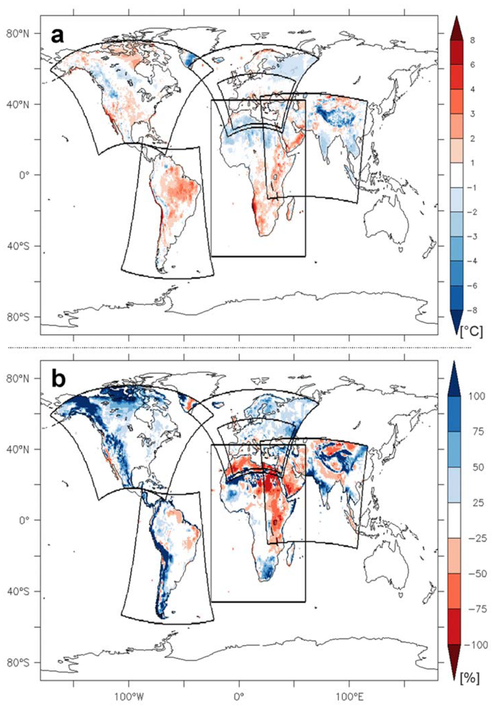
Figure 3(a). Regions where the model is doing relatively well can be found in Europe, western Africa, eastern North America and south eastern South America. In these regions, the temperatures do not deviate more than one degree from observations. Taking into consideration that the annual mean temperature may not reveal all regional or temporal shortcomings, there are only a few regions where the model shows problematic behavior. First, the Amazonian forest area in South America has a considerable warm bias around 2 to 3 °C over a large area. The reasons are not yet fully understood but it may be attributed to insufficient local moisture recycling, especially in the dry season in the boreal summer. Here, it seems that the one-layer soil water storage of REMO does not take into account the buffering effect of water in deeper layers of the soil that may be accessed for transpiration by the vegetation in dry season, as investigated in the study of Kleidon and Heimann [
27]. Second, the strong cold bias in the Himalayan region may be a model artifact to some degree, but also the observation data sparseness in that region seems to play a major role in emphasizing this feature. Third, the distinct warm bias north of the Hudson Bay in North America may have two reasons. One reason is the insufficient temperature representation of the Hudson Bay water body and the other may be concerned with an insufficient snow masking in that region.
Figure 3.
(a) Differences of simulated and observed (CRU) annual mean air temperature (2 m height) in [°C]; (b) Relative annual mean differences between simulated and observed (CRU) precipitation in [%]. The period considered is 1989 to 2006.
Figure 3.
(a) Differences of simulated and observed (CRU) annual mean air temperature (2 m height) in [°C]; (b) Relative annual mean differences between simulated and observed (CRU) precipitation in [%]. The period considered is 1989 to 2006.
In
Figure 3(a), strong surface warm biases are detected in coastal areas of Baja California (North America), Santiago de Chile up to Ecuador (South America) and the Namib Desert (Africa). In particular, the temperatures alongshore the Benguela Ocean current are far too warm all year round. The common characteristics of these regions are the upwelling of cold water and the subsidence of warm and dry air, driven by the Hadley circulation. This creates a thin inversion layer where stratocumulus clouds are formed. The simulated warm bias could be related to the misrepresentation of stratocumulus clouds and therefore an overestimation of radiation input to the surface as it already has been discussed in Haensler
et al. [
28] for the southern African region and/or wrong sea surface temperatures from the driving ERA-Interim data set [
29,
30].
In
Figure 3(b), relative annual mean precipitation differences between simulated and observed (CRU) precipitation are shown. A prominent systematic feature is the occurrence of biases above hundred percent in dry regions. These can be related to the standardization method that is applied to the data and to the division by small values resulting in huge percentage differences. Apart from that, a prominent bias is the strong overestimation of rainfall up to 100% in the western mountain chains in the Americas and in the North American Arctic regions. To some degree, the latter error may be connected to the undercatch of the observing stations, which can lead to underestimation of precipitation in the annual observations by up to 40% [
23]. Yang
et al. [
31] show that the correction factors for precipitation can reach monthly values of more than 100% during the winter season at high latitudes. This is the period in which REMO precipitation bias in comparison to CRU is highest (not shown). Regions, where precipitation is underestimated by up to 75%, are located in eastern and northern Africa and on the Arabic Peninsula. The distinct dipole error pattern over India with underestimation of precipitation in the northeast and overestimation over central India can be attributed to insufficiently characterized monsoon features and flow directions. In other regions, the model simulates the precipitation in Europe, eastern North America, eastern South America, western and south-western Africa quite well.
A general systematic inverse correlation of temperature bias to precipitation bias is not directly detected. In some regions such as India and eastern Central Europe, this assumption is true where a wet bias corresponds to a cold bias. In most regions, the picture looks quite non-systematic. For example, a warm bias corresponds to a wet bias in southern Africa and arctic North America. Inversely, a cold bias is associated with a dry bias in North Africa.
As mentioned earlier that to a large extent, the evaluation of the model is hampered by the lack of observational data. An example in this regard is the West Asian’s wet bias in REMO for the climate type Dc for the month December–February as given in
Table 2. This region receives considerable amount of precipitation from western disturbances in these months, and it can be seen in
Figure 2 that most of this climate type is present in Afghanistan or at very high altitudes over Pakistan. The lack of appropriate observational data in these regions is responsible for this particular bias.
One of the main objectives of the CORDEX experiment is to produce high-resolution regional climate change information as input to climate impact research and adaptation work. Many impact models need such information on river basin scale. Therefore in this study, the annual cycles of precipitation and temperature (2 m height) over the representative river basins for each domain are analysed in REMO. The selection of river basins is done acording to the study by Dai
et al. [
32], in which they conducted the trend analysis for world’s top 24 rivers [
33] from 1948 to 2004. Here we have selected only those river basins that show significant positive or negative trends according to Dai
et al. [
32]. However, since there is no river basin in the European or Mediterranean domain showing any significant trend, the Danube river basin that is the largest European river basin is selected. In the present study, the masks for different river basins are derived from Hagemann and Duemenil [
34].
Table 2.
Standard deviation for monthly values of temperature (T: upper part) and precipitation (P: lower part) between CRU observations (O: black) and REMO (M: red) during different seasons for all climate types and regions inside the period 1989–2006.
Table 2.
Standard deviation for monthly values of temperature (T: upper part) and precipitation (P: lower part) between CRU observations (O: black) and REMO (M: red) during different seasons for all climate types and regions inside the period 1989–2006.
| T | O | M | O | M | O | M | O | M | O | M | O | M | O | M | O | M | O | M | O | M | O | M | O | M |
|---|
| DJF | Ar | Aw | Bs | Bw | Cr | Cs | Cw | Dc | Do | Ec | Eo | FT |
| Eu | | | | | | | | | | | 1.2 | 0.9 | | | 2.3 | 2.4 | 1.1 | 1.1 | 3.1 | 3.0 | 2.0 | 2.2 | | |
| Med | | | | | | | 1.2 | 1.2 | | | 1.1 | 1.0 | | | 2.1 | 2.2 | 1.2 | 1.2 | | | | | | |
| WA | | | 1.0 | 1.8 | 1.5 | 1.6 | 1.4 | 1.4 | | | | | 1.2 | 1.9 | 1.6 | 1.7 | 1.5 | 1.5 | | | | | 1.4 | 1.8 |
| Afr | 0.6 | 0.8 | 0.7 | 0.9 | 0.7 | 0.7 | 1.0 | 1.1 | 0.6 | 0.6 | | | | | | | | | | | | | | |
| NA | | | | | 1.5 | 1.3 | | | | | | | | | 2.4 | 2.0 | | | 2.7 | 3.1 | | | 2.8 | 3.1 |
| SA | 0.4 | 0.8 | 0.3 | 0.8 | 0.6 | 0.6 | | | 0.7 | 0.9 | | | | | | | 0.8 | 1.0 | | | | | | |
| MAM | Ar | Aw | Bs | Bw | Cr | Cs | Cw | Dc | Do | Ec | Eo | FT |
| Eu | | | | | | | | | | | 2.9 | 2.6 | | | 5.3 | 5.4 | 2.8 | 2.9 | 5.7 | 5.6 | 4.0 | 3.9 | | |
| Med | | | | | | | 3.7 | 4.2 | | | 3.0 | 2.8 | | | 5.0 | 5.0 | 2.9 | 2.8 | | | | | | |
| WA | | | 1.3 | 1.2 | 4.5 | 4.7 | 4.4 | 4.5 | | | | | 2.5 | 2.4 | 4.6 | 4.2 | 4.4 | 4.2 | | | | | 3.8 | 4.5 |
| Afr | 0.5 | 0.6 | 0.7 | 0.7 | 0.6 | 0.6 | 2.3 | 2.5 | 0.5 | 0.6 | | | | | | | | | | | | | | |
| NA | | | | | 3.7 | 3.6 | | | | | | | | | 5.2 | 4.9 | | | 7.3 | 7.6 | | | 7.3 | 7.8 |
| SA | 0.4 | 0.7 | 0.6 | 0.8 | 2.0 | 2.1 | | | 2.5 | 2.6 | | | | | | | 2.7 | 2.9 | | | | | | |
| JJA | Ar | Aw | Bs | Bw | Cr | Cs | Cw | Dc | Do | Ec | Eo | FT |
| Eu | | | | | | | | | | | 1.5 | 1.7 | | | 1.3 | 1.3 | 1.5 | 1.5 | 1.8 | 2.0 | 1.6 | 1.7 | | |
| Med | | | | | | | 1.0 | 1.3 | | | 1.5 | 1.8 | | | 1.4 | 1.4 | 1.5 | 1.6 | | | | | | |
| WA | | | 0.7 | 0.9 | 0.7 | 0.6 | 0.6 | 0.6 | | | | | 0.5 | 0.8 | 1.3 | 1.4 | 1.0 | 1.1 | | | | | 1.1 | 1.0 |
| Afr | 0.5 | 0.5 | 0.5 | 0.5 | 0.5 | 0.7 | 0.5 | 0.3 | 0.6 | 0.9 | | | | | | | | | | | | | | |
| NA | | | | | 1.1 | 0.9 | | | | | | | | | 1.5 | 1.9 | | | 1.4 | 1.3 | | | 1.9 | 1.3 |
| SA | 0.4 | 1.1 | 0.6 | 1.4 | 1.0 | 1.1 | | | 1.2 | 1.2 | | | | | | | 1.0 | 1.2 | | | | | | |
| SON | Ar | Aw | Bs | Bw | Cr | Cs | Cw | Dc | Do | Ec | Eo | FT |
| Eu | | | | | | | | | | | 3.7 | 3.5 | | | 5.3 | 5.3 | 3.7 | 3.7 | 6.6 | 6.3 | 4.3 | 3.8 | | |
| Med | | | | | | | 4.6 | 5.4 | | | 3.8 | 3.9 | | | 5.1 | 5.0 | 3.8 | 3.7 | | | | | | |
| WA | | | 1.1 | 1.5 | 4.6 | 4.8 | 4.6 | 4.9 | | | | | 2.6 | 3.3 | 5.3 | 5.0 | 4.8 | 4.9 | | | | | 5.4 | 6.3 |
| Afr | 0.6 | 0.5 | 0.6 | 0.5 | 0.6 | 0.6 | 2.7 | 3.4 | 1.0 | 1.5 | | | | | | | | | | | | | | |
| NA | | | | | 4.7 | 4.3 | | | | | | | | | 5.8 | 5.6 | | | 7.4 | 7.5 | | | 7.0 | 7.1 |
| SA | 0.4 | 0.7 | 0.5 | 0.9 | 1.6 | 1.6 | | | 1.9 | 1.7 | | | | | | | 2.2 | 2.2 | | | | | | |
| P | O | M | O | M | O | M | O | M | O | M | O | M | O | M | O | M | O | M | O | M | O | M | O | M |
| DJF | Ar | Aw | Bs | Bw | Cr | Cs | Cw | Dc | Do | Ec | Eo | FT |
| Eu | | | | | | | | | | | 34.5 | 36.6 | | | 9.7 | 14.8 | 21.4 | 23.8 | 8.1 | 10.1 | 23.0 | 27.1 | | |
| Med | | | | | | | 3.8 | 2.5 | | | 25.9 | 26.9 | | | 10.4 | 12.5 | 21.0 | 20.9 | | | | | | |
| WA | | | 13.7 | 18.3 | 5.6 | 10.0 | 3.3 | 7.3 | | | | | 9.1 | 9.7 | 9.6 | 15.1 | 8.8 | 15.3 | | | | | 5.3 | 7.3 |
| Afr | 18.5 | 26.2 | 10.5 | 9.5 | 12.3 | 10.2 | 2.2 | 2.1 | 16.2 | 14.6 | | | | | | | | | | | | | | |
| NA | | | | | 7.9 | 16.2 | | | | | | | | | 10.9 | 13.6 | | | 6.0 | 6.8 | | | 5.8 | 8.0 |
| SA | 41.4 | 33.6 | 24.7 | 35.5 | 22.2 | 26.8 | | | 29.4 | 35.9 | | | | | | | 9.7 | 15.0 | | | | | | |
| MAM | Ar | Aw | Bs | Bw | Cr | Cs | Cw | Dc | Do | Ec | Eo | FT |
| Eu | | | | | | | | | | | 14.8 | 18.4 | | | 10.4 | 13.7 | 15.1 | 17.2 | 9.2 | 15.1 | 15.6 | 19.7 | | |
| Med | | | | | | | 3.9 | 2.6 | | | 14.2 | 15.6 | | | 11.4 | 12.6 | 15.4 | 17.4 | | | | | | |
| WA | | | 53.1 | 82.2 | 5.7 | 7.0 | 4.5 | 5.1 | | | | | 48.6 | 82.2 | 12.7 | 15.9 | 12.8 | 17.2 | | | | | 11.8 | 10.5 |
| Afr | 22.9 | 27.7 | 13.9 | 11.6 | 8.6 | 9.1 | 1.7 | 2.7 | 38.7 | 27.5 | | | | | | | | | | | | | | |
| NA | | | | | 11.0 | 15.0 | | | | | | | | | 14.7 | 16.2 | | | 6.9 | 8.7 | | | 4.1 | 8.3 |
| SA | 34.1 | 34.9 | 44.3 | 55.8 | 29.8 | 43.6 | | | 34.0 | 42.0 | | | | | | | 16.6 | 23.1 | | | | | | |
| JJA | Ar | Aw | Bs | Bw | Cr | Cs | Cw | Dc | Do | Ec | Eo | FT |
| Eu | | | | | | | | | | | 8.2 | 9.9 | | | 13.2 | 14.0 | 14.7 | 12.2 | 13.4 | 15.6 | 17.4 | 18.1 | | |
| Med | | | | | | | 0.6 | 0.3 | | | 5.9 | 5.7 | | | 14.9 | 14.3 | 14.4 | 13.1 | | | | | | |
| WA | | | 39.9 | 67.8 | 20.7 | 23.5 | 5.4 | 7.1 | | | | | 49.2 | 43.4 | 8.9 | 9.8 | 12.0 | 15.9 | | | | | 15.5 | 13.4 |
| Afr | 19.2 | 20.6 | 15.4 | 11.2 | 18.5 | 15.1 | 9.7 | 6.7 | 3.6 | 2.9 | | | | | | | | | | | | | | |
| NA | | | | | 13.4 | 12.6 | | | | | | | | | 12.9 | 13.0 | | | 9.4 | 8.7 | | | 8.8 | 10.5 |
| SA | 38.4 | 40.5 | 8.9 | 9.5 | 5.3 | 5.0 | | | 21.0 | 19.6 | | | | | | | 18.9 | 27.9 | | | | | | |
| SON | Ar | Aw | Bs | Bw | Cr | Cs | Cw | Dc | Do | Ec | Eo | FT |
| Eu | | | | | | | | | | | 29.7 | 31.3 | | | 13.2 | 17.1 | 20.1 | 18.9 | 11.0 | 18.4 | 18.8 | 24.6 | | |
| Med | | | | | | | 6.5 | 2.6 | | | 24.2 | 24.6 | | | 14.4 | 15.9 | 20.3 | 18.9 | | | | | | |
| WA | | | 70.0 | 121.8 | 13.2 | 29.1 | 2.4 | 6.2 | | | | | 73.1 | 63.7 | 10.2 | 12.5 | 11.9 | 16.6 | | | | | 18.3 | 22.6 |
| Afr | 26.3 | 27.4 | 20.0 | 23.2 | 10.2 | 13.3 | 4.1 | 4.3 | 28.8 | 22.3 | | | | | | | | | | | | | | |
| NA | | | | | 19.4 | 21.8 | | | | | | | | | 10.0 | 13.6 | | | 11.5 | 12.8 | | | 8.1 | 11.4 |
| SA | 27.5 | 32.1 | 30.6 | 34.1 | 20.4 | 29.7 | | | 29.5 | 37.2 | | | | | | | 10.3 | 16.3 | | | | | | |
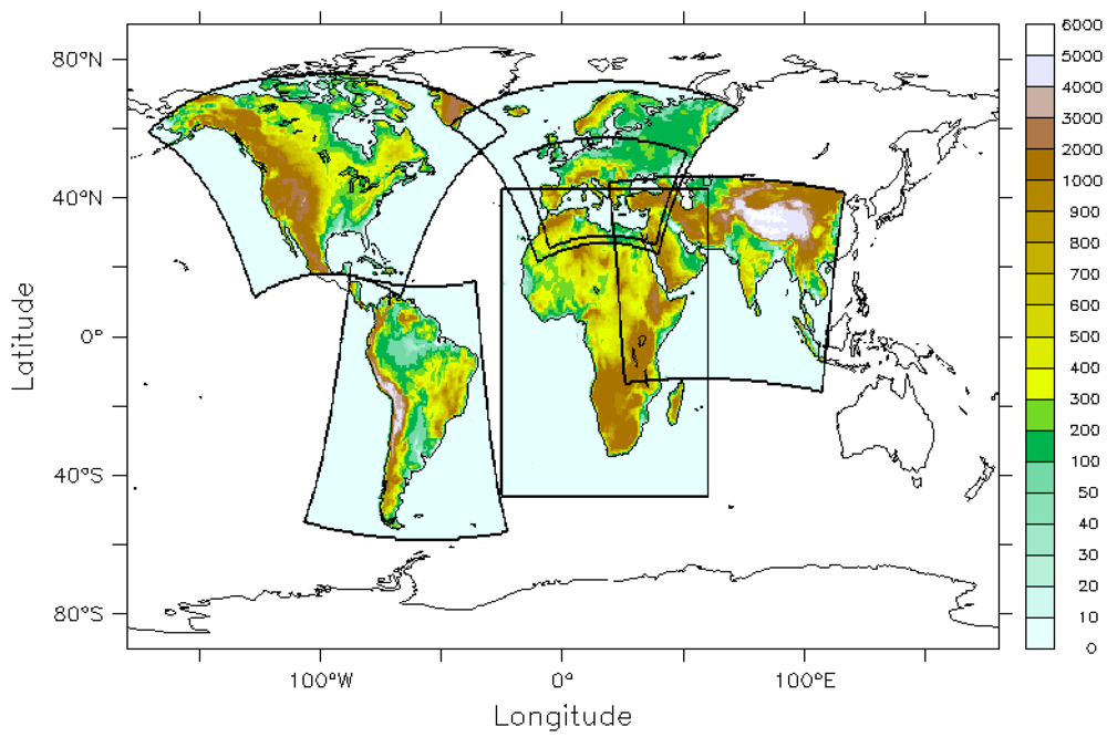
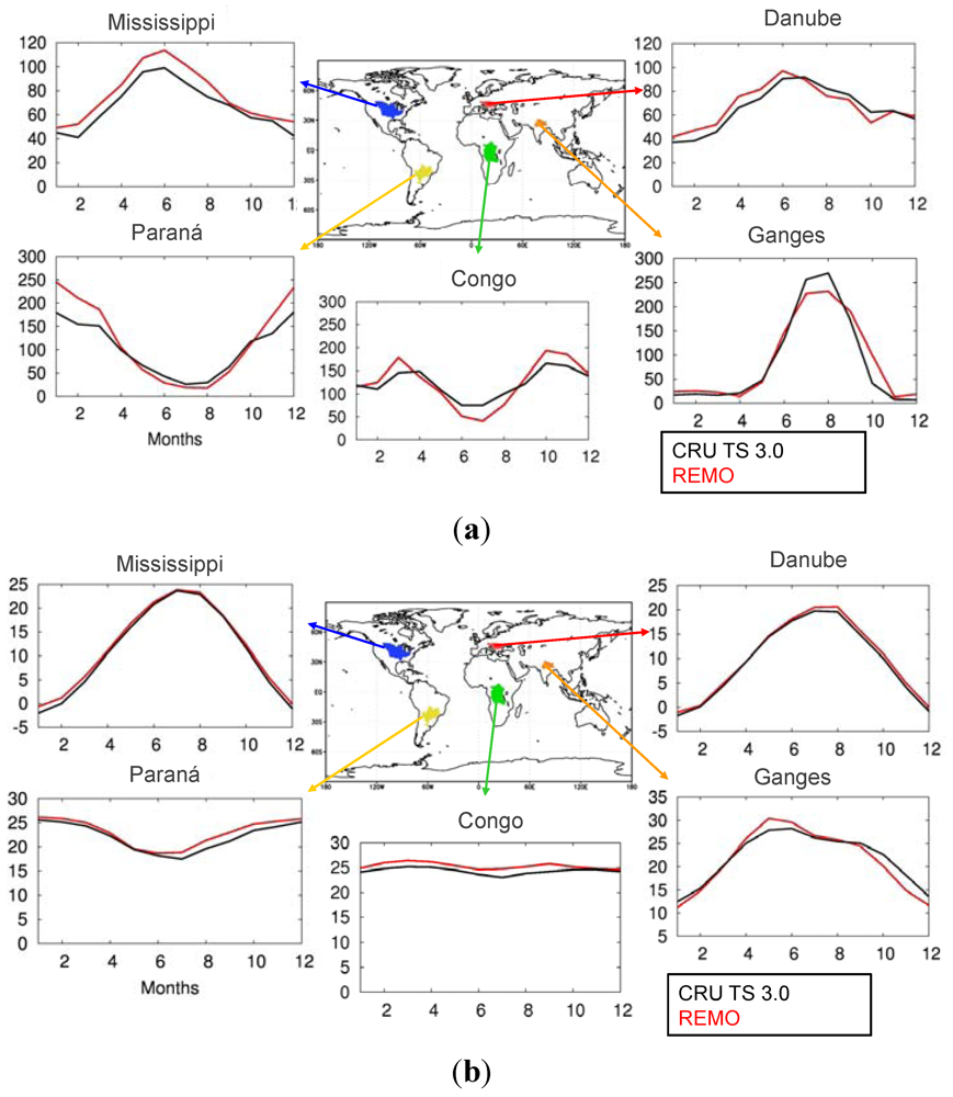
Figure 4 shows the annual cycles of precipitation and temperature for different river basins of each domain. It is evident from these figures that REMO has simulated the annual cycles of both the variables very well. Considering the fact that according to Köppen-Trewartha (
Figure 2) these basins are situated in different climate types with the Congo being typically tropical, Paraná and Ganges being subtropical and Danube and Mississippi mainly having temperate climate, the model’s performance appears even more satisfactory. As shown in
Figure 4(a), REMO has captured the dual maxima of precipitation of the Congo basin, which is associated with the annual movement of the Intertropical Convergence Zone (ITCZ). However the simulated seasonality over the Paraná Basin is larger than the corresponding observed seasonal cycle, with higher (less) amounts of precipitation during the rainy (dry) season. Over the west Asian domain, considering it is a “notoriously difficult to predict” nature of South Asian Summer Monsoon [
35], REMO has captured the seasonality between wet and dry season quite well with a small dry and wet bias in monsoon and post monsoon months, respectively. Also for Danube and Mississippi river basins, the model results are very similar to observations with differences lower than 10 mm/month in each month for both basins. For the annual cycle of temperature (
Figure 4(b)), it can be seen that model has captured the strong seasonality in the case of Danube, Mississippi and Ganges, and weak seasonality for the case of Congo and Paraná basins quite well. The maximum difference of around 2 °C occurs in a few months for Paraná and Ganges, however for other basins it remains within 1 °C difference.
Figure 4.
Annual cycles of (a) Precipitation [mm/month] (b) Temperature [°C] of selected catchments over each domain. Black and Red curves denote the CRU observations and REMO results respectively. The period considered is 1989 to 2006.
Figure 4.
Annual cycles of (a) Precipitation [mm/month] (b) Temperature [°C] of selected catchments over each domain. Black and Red curves denote the CRU observations and REMO results respectively. The period considered is 1989 to 2006.
4.2. Temperature Precipitation Relationship
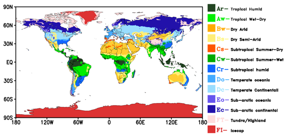
The precipitation-temperature relationship plots according to the Köppen-Trewartha climate classification types both for REMO and CRU data are discussed in this subsection. The area for each climate type is defined using Köppen-Trewartha climate classification based on CRU data as shown in
Figure 2. This relationship is calculated for each domain and for each climate type.
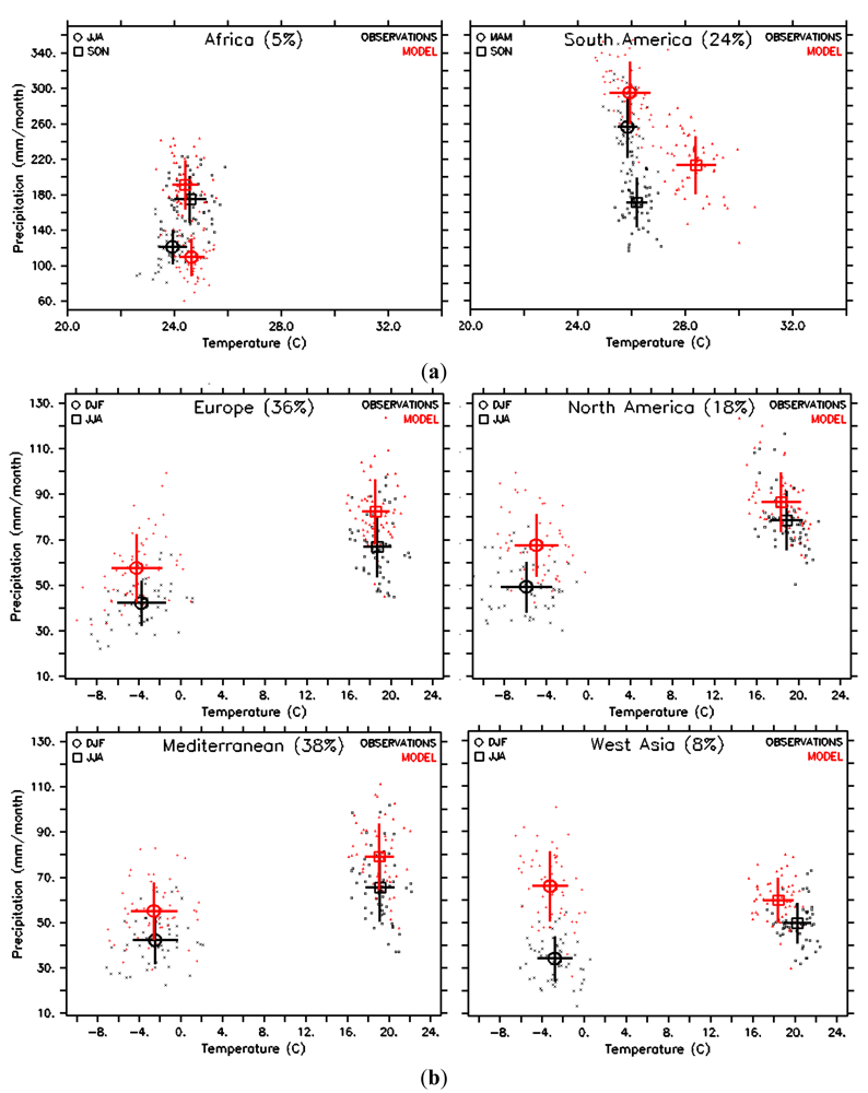
Figure 5 shows a subset of the results of monthly values for precipitation-temperature regimes in different regions during different seasons. The two climate types shown are the tropical humid climate (Ar, as listed in
Figure 2) of South America and Africa (
Figure 5(a)) and the temperate continental climate (Dc) of Europe, Mediterranean, North America and West Asia (
Figure 5(b)). The seasons are selected relative to the maximum and minimum temperature values at each region.
The clusters of observational and model data explain the intraseasonal variability, and they are quantified by the standard deviation. These values are summarized for all climate types in
Table 2. The clusters’ shape, given by the temperature and precipitation spread data, can be seen as a characteristic of the climate type. It varies along the seasons and regions, accordingly. As observed for the Dc climate type, which has similar characteristics with subtropical summer-wet (Cw) climate type, the subarctic continental (Ec) climate type and the tundra/highland climate type (FT) (not shown), the intraseasonal variability of temperature is larger in December, January, February (above 10 °C) than in the June, July, August season (approximately 4 °C). In the case of precipitation, climate types such as Ar (shown in
Figure 5(a)) and the tropical wet-dry (Aw and As) climate type have values between 100 to 360 mm/month during rainy seasons. This variability is larger compared to the dry seasons of Aw, the dry semi-arid (Bs) climate type and the dry arid (Bw) climate type with monthly precipitation values between 10 to 40 mm/month. This is indicated as well by the standard deviation values at
Table 2. The standard deviation from the model data is comparable to the observations for the climate type Dc, with the exception of the North American region. In general, the difference of the standard deviation values between the model and observational data is smaller at the climate types located in the midlatitudes than in the low and high latitudes.
Figure 5 also shows the interseasonal differences given by the differences in the precipitation-temperature regimes through the two seasons. This is expressed as two different clusters of data in each panel. The interseasonal differences for each climate type depends on several features at local, mesoscale and synoptic processes scales. In climate types representative of lower latitudes (e.g., Ar), small interseasonal differences for temperature (less than 1 °C) are observed. However, strong interseasonal changes in precipitation are observed where the range is between 60 to 100 mm/month (
Figure 5(a)). Moving polewards, these interseasonal temperature changes become more noticeable such as in midlatitude climate types (e.g., Dc). Moving further towards the higher latitudes, these interseasonal temperature-precipitation differences become even larger with greater than 10 °C for temperature and 40 to 200 mm/month for precipitation (figure not shown). The differences on the regimes for the same climate type in different regions are a consequence of the climate type classification adopted in this study.
Köppen and Trewartha classification in comparison to other climate classification such as Köppen and Geiger [
36] have established lower threshold values that define the climate types, and therefore bring together separated climate subtypes from Köppen and Geiger classification. The inversion of the warm or cold seasons (for climate types such as Aw, the subtropical humid (Cr) climate type and the temperate oceanic (Do) climate type) is a consequence of the geographical location situated on opposite hemispheres for that climate types.
Biases can be analyzed through the differences on the mean values. Reiterated bias appear on different climate types, high latitudes climate types such as Dc, Ec and FT show larger positive bias on precipitation compared to Ar. It is difficult to find a general attribution to this common bias. Misrepresentation of different processes could lead to the same signal model errors. Part of the bias on extreme climates like FT, could be attributed to the quality of the observation dataset as well. Over those areas, the dataset mainly presents two problems: low density of stations distribution and underestimation in instrument measurements due to the precipitation undercatch as a consequence of large wind speed. Temperatures in general are well represented, only larger biases around 2 °C are observed for tropical climate types (Ar and Aw) types, mainly at the Amazon region in South America. These biases, as explained in the previous section, take place during September, October, November months. At these latitudes, convection processes are very active and therefore the physical part of the model considered more difficult to reproduce than the dynamical part, might contribute to the biases.
Figure 5.
Seasonal Climate types Ar (a) and Dc (b). Each group of data represents observations and model results. Each dot represents the monthly mean value of precipitation and temperature in each month of the corresponding season. Seasons at each plot are identified by their different temperature-precipitation regime that results in two clusters of two groups of data. The seasons were chosen to represent the periods in which precipitation and/or temperature maximum and minimum values take place throughout the year, in this way, maximal annual amplitude is represented, note that the Ar climate type in Africa has two wet periods in the year (March, April, May and September, October, November), then June, July, August was selected as the dry season. The mean for both variables, temperature and precipitation, is represented by a square or a circle for each season. The bars represent the standard deviation. The percentage values correspond to the area covered by the climate type with respect to the total land area in the region. The period considered is 1989 to 2006.
![Atmosphere 03 00181 g005]()
4.3. PDF Skill Score
In this section, the results of the PDF skill score method are shown to evaluate the transferability of the model. Altogether there are 30 regions of different climate type and model domains on which the ranking of scores is based. Each skill score is calculated based on the comparison with CRU data in the same subregion. Using the climate classification types allows a quantitative measure of the model’s skill unlike previous studies wherein model results are subdivided according to unphysical criteria such as administrative borders or regular boxes [
7].
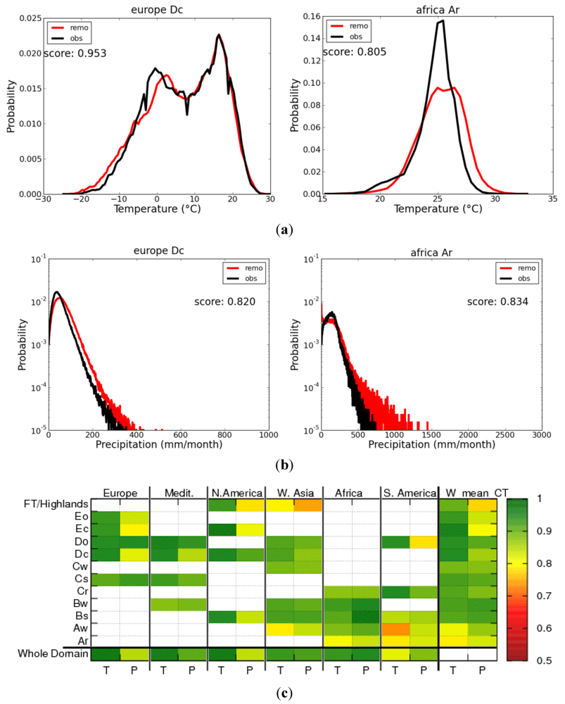
The continents are subdivided into different regions according to climate types. In regions with the same climate type, the characteristics in precipitation and temperature distributions are alike. For instance, in continental temperate climate (Dc) regions in Europe (
Figure 6(a)), the temperature distribution based on the gridded observational dataset, tends to be bimodal. The maximum probabilities are at around 0 and 20 °C. The observed extreme monthly mean precipitation values can reach up to 700 mm/month. In domains with this climate type (Europe, Mediterranean, West Asia, and North America), the model represents well the bimodality of the temperature distribution and thus has high skill scores (more than 0.9). However the model overestimates the occurrence of high values of monthly mean precipitation. The good representation of the more frequent but lower precipitation rates still leads to a high skill score (more than 0.8).
Figure 6.
Probability density function (PDF) Skill scores for (a) temperature (T) and (b) precipitation (P). Example PDF results in selected regions: temperate continental climate (Dc) over Europe (a and b, left); and tropical humid climate (Ar) over Africa (a and b, right). The temperature and precipitation PDF curves for the observed (black) and simulated (red) distributions are shown. The precipitation plots are in logarithmic scale and the probability values shown are equal or greater than 10−5. (c) Summary of the PDF skill scores for all climate types. The last column shows the weighted mean of PDF skill scores (W_mean_CT) across different domains for every climate type. The period considered is 1989 to 2006.
In contrast to the relatively high skill score in the temperate climate region discussed above, relatively low skill scores especially in temperature can be found in regions with the tropical humid climate type (Ar) in Africa and South America (
Figure 6(b)). The observations show a unimodal temperature distribution which peaks at around 25 °C. The distribution of the simulated monthly mean temperature values shows a similar behavior but underestimates their frequency between 24 °C and 28 °C. In addition, the model also simulates higher probabilities for temperature values of more than 27 °C. This can also be seen in
Section 4.1, where the warm bias of the model in comparison with CRU data can be observed.
Skill scores for all climate types and all regions are summarized in the table in
Figure 6(c). High skill scores (relative to the whole table) are represented in green, while lower skill scores are represented in red. In general it can be seen that for temperature, skill scores are higher for the more temperate climate types than for the more extreme climate types such as tundra (FT), tropical wet-dry (Aw) and tropical humid (Ar). For precipitation a similar behavior can be observed. High skill scores in precipitation are found in temperate climates except for the temperate oceanic (Do) climate type in South America. In regions with low skill score, the model tends to simulate higher precipitation rates and higher occurrence of these rates compared to CRU data.
The last row and the last column in
Figure 6(c) represent the overall skill of REMO for all domains and climate types, respectively. The skill of the model in each domain is calculated using all monthly precipitation and temperature values disregarding the climate types. In evaluating the skill of the model according to the different climate types, the PDF skill score is calculated using the weighted mean of climate types’ scores at different domains. In this figure, the performance of REMO for temperature is best in the European, Mediterranean and North American domain, while it is comparatively low in South America. Precipitation shows highest skill scores for the Mediterranean, African and West Asian regions.
The scores for temperature are high in the midlatitude climate types and the lowest are in the tropical climate types (Ar, Aw). In the case of precipitation, skill scores are lowest for arctic and tundra/highland climate types. The other climate types are simulated well by the model.


