Numerical Simulation of the Global Neutral Wind System of the Earth’s Middle Atmosphere for Different Seasons

Abstract

A non-hydrostatic model of the global neutral wind system of the Earth’s atmosphere, developed earlier, is utilized to simulate the large-scale global circulation of the middle atmosphere for conditions of different seasons. In the model calculations, not only the horizontal components, but also the vertical component of the neutral wind velocity, are obtained by means of a numerical solution of a generalized Navier-Stokes equation for compressible gas, so the hydrostatic equation is not applied. Moreover, the global temperature field is assumed to be a given distribution, (i.e., the input parameter of the model) and obtained from one of the existing empirical models. The results of simulation indicate that the horizontal non-uniformity of the neutral gas temperature, which is distinct in different seasons, ought to considerably influence the formation of the global neutral wind system in the middle atmosphere, in particular, the large-scale circumpolar vortices of the northern and southern hemispheres.

1. Introduction

Within the past three decades, several general circulation models of the lower and middle atmosphere have been developed (for example, see [1,2,3,4,5,6,7,8,9,10,11]). It can be noticed that the existing general circulation models of the lower and middle atmosphere may be successfully utilized for the simulation of slow climate changes. Unfortunately, these models cannot produce the vertical atmospheric wind with an acceptable accuracy. The fact is that the momentum equation for the vertical velocity is omitted in commonly-used general circulation models, and the vertical velocity is obtained with the help of a simple hydrostatic equation. Similarly, both the global circulation models of the thermosphere and coupled thermosphere-ionosphere global models, such as [12,13,14,15,16,17], cannot produce the vertical component of the neutral wind with an acceptable accuracy because of utilizing the simple hydrostatic equation. As a consequence of this simplification, such models do not provide an ability to simulate the large-scale global circulation in all regimes, in particular, under disturbed conditions. As is well known, the global models just mentioned produce the vertical component of the wind velocity having the values of several centimeters per second at levels of the lower thermosphere. However, the observed vertical velocity is known to amount up to some tens m/s at levels of the mesosphere and lower thermosphere in high latitude regions (see [18,19,20,21,22]). Thus, it is necessary to use more complex general circulation models in order to describe the vertical transport more adequately and to simulate the transient large-scale global circulation of the middle atmosphere and lower thermosphere.

Not long ago, a new non-hydrostatic model of the global neutral wind system of the Earth’s atmosphere was developed in the Polar Geophysical Institute (PGI) [23,24]. This model allows the calculation of the three-dimensional global distributions of the zonal, meridional and vertical components of the neutral wind at levels of the troposphere, stratosphere, mesosphere and lower thermosphere, with the hydrostatic equation not being applied. This model has been utilized in order to simulate the global circulation of the middle atmosphere for conditions corresponding to summer in the northern hemisphere (see [23,24]). It has been found in these studies that the global distributions of the neutral wind, calculated for the summer period in the northern hemisphere, in particular the large-scale circumpolar vortices, are consistent with the planetary circulations of the atmosphere obtained from observations.

The purpose of the present work is to continue these studies and to investigate numerically, using the non-hydrostatic model of the global neutral wind system [23,24], how the horizontal non-uniformity of the neutral gas temperature affects the formation of the middle atmosphere circulation, in particular the large-scale circumpolar vortices of the northern and southern hemispheres, for conditions corresponding to four different seasons (winter, spring, summer, and autumn).

2. Mathematical Model

In the present study, the non-hydrostatic model of the global neutral wind system in the Earth’s atmosphere, developed earlier in the PGI [23,24] is utilized. This model fundamentally differs from existing global circulation models of the atmosphere in two ways. Firstly, the model does not include the pressure coordinate equations of atmospheric dynamic meteorology, in particular, the hydrostatic equation. Instead, the vertical component of the neutral wind velocity is obtained by means of a numerical solution of the appropriate momentum equation, with no single term in this equation being omitted. Thus, three components of the neutral wind velocity are obtained by means of a numerical solution of the Navier-Stokes equation for compressible gas. Therefore, the utilized mathematical model has the potential to describe the global neutral wind system under disturbed conditions because of applying the momentum equation for the vertical component of the neutral wind velocity.

Secondly, the utilized model does not include the internal energy equation for the neutral gas. Instead, the temperature field is assumed to be a given distribution, i.e., the input parameter of the model, and obtained from one of the existing empirical models. This peculiarity of the utilized model is justified by the following circumstances. It is known that the temperature distributions, calculated by using the global circulation models at levels of the troposphere, stratosphere, mesosphere and lower thermosphere, as a rule, differ from the observed distributions of the atmospheric temperature. These differences are due to an unsatisfactory accuracy of the global circulation models for the temperature regime of the neutral gas. Due to complexities and uncertainties in various chemical-radiational heating and cooling rates, there is no reason to expect an exact correspondence between the calculated and measured temperatures of the neutral gas. Despite considerable research, the problem of the atmospheric temperature simulation in the lower and middle atmosphere is not completely solved.

On the other hand, over the past few years, empirical models of the global atmospheric temperature field in the middle atmosphere have been developed which have a satisfactory accuracy (for example, see [25,26]). The non-hydrostatic model allows the application of the latter empirical models of the neutral gas temperature for the simulation of the global neutral wind system in the Earth’s middle atmosphere.

The global circulation of the atmosphere is described in a spherical coordinate system (r, β, φ), rotating together with the Earth, with r, β and φ being the radius, latitude and longitude, respectively. For solving the system of Equations, utilized in the mathematical model, the finite-difference method is applied. The vertical, meridional and zonal components of the neutral wind velocity (v_r, v_β and v_φ, respectively) obey the generalized Navier-Stokes Equations for compressible gas:

(1)

(2)

(3)

where ρ is the neutral gas density, p is the pressure, Ω is the Earth’s angular velocity, r₀ is the radius of the Earth at the pole, g₀ is the gravity acceleration at the pole at sea level, , , and are vector components of the acceleration due to elastic collisions with the ion gas, and τ_rr, τ_ββ,τ_φφ, τ_rφ, τ_rβ, and τ_φβ are the components of the extra stress tensor which are given by the rheological Equation of state or constitutive Equation (also called “law of viscous friction”). Namely, is composed of a Newtonian part, , and a complementary part, :

(4)

The former tensor, , is given by the well-known Newton’s law of viscous friction,

(5)

where μ₀ is the coefficient of molecular viscosity, whose dependence on temperature is assumed to obey the Sutherland’s law, and is the tensor defined as

(6)

where is the strain rate tensor, is the unit tensor, and denotes the trace of a tensor. The complementary stress tensor, is supposed to be determined by a small-scale turbulence having the scales equal and less than the steps of the finite-difference approximation. It is assumed that this tensor represents the effect of the turbulence on the mean flow and is given by an expression, analogous to the Newton’s law of viscous friction, Equation (5), with the scalar coefficient of viscosity, μ₀, being replaced by three distinct coefficients describing the eddy viscosities in the directions of the base vectors of the corresponding spherical coordinate system. For computing the eddy viscosities, one of the numerous existing turbulence models may be applied. In the utilized mathematical model, the turbulence theory of Obukhov [27] is applied for calculating the eddy viscosities.

The utilized mathematical model contains the continuity Equation of the neutral gas which can be written as:

(7)

Besides, the state equation for an ideal gas is used in the mathematical model for obtaining the connection between the pressure and temperature of the neutral gas.

The system of equations containing the momentum equations for the vertical, meridional and zonal components of the neutral gas velocity, Equations (1–3), as well as the continuity equation, Equation (7), is numerically solved in a global layer surrounding the Earth. The lower boundary of this layer is the Earth’s surface, which is assumed to be an oblate spheroid whose radius at the equator is more than that at the pole. The upper boundary of this layer is a sphere with an altitude of 126 km at the equator.

At the lower boundary, the velocity vector is determined from the no-slip conditions on the ground. Simulation results presented in this paper are obtained using the following condition at the upper boundary:

(8)

The utilized mathematical model allows us to calculate three-dimensional global distributions of the vertical, meridional and zonal components of the neutral wind and neutral gas density. As pointed out previously, the finite-difference method is applied for solving the system of equations. The calculated parameters are determined on a 1° grid in both longitude and latitude. The height step is non-uniform and does not exceed the value of 1 km. More complete details of the mathematical model can be found in [23,24].

3. Results and Discussion

The utilized mathematical model of the global neutral wind system can be used for different geomagnetic, solar cycle and seasonal conditions. For the present study, calculations were performed for conditions corresponding to four different dates, namely, 16 January, 16 April, 16 July, and 16 October, which, in the northern hemisphere, belong to winter, spring, summer and autumn respectively. Calculations were made for moderate solar activity (F_10.7 = 101) and low geomagnetic activity (Kp = 1). The steady-state distributions of the atmospheric parameters were obtained for the four considered dates at 10.30 UTC. The temperature distributions, corresponding to this moment, were taken for each day from the NRLMSISE-00 empirical model [26].

To investigate how the global distribution of the neutral gas temperature, corresponding to various seasons, affects the formation of the middle atmosphere circulation, the numerical solutions of the system of equations, described above, were obtained by assuming that the boundary conditions and inputs to the model are time-independent and correspond to 10.30 UTC. The simulation results are partly shown in Figure 1, Figure 2, Figure 3, Figure 4. The given temperature distributions, obtained for the altitude of 50 km, are shown on the top panels of Figure 1, Figure 2, Figure 3, Figure 4. It is seen that the planetary distributions of the atmospheric temperature are non-uniform and distinct in different seasons.

Figure 1. The distributions of the given neutral gas temperature (top panel), vector of the calculated horizontal component of the neutral wind velocity (middle panel), and calculated vertical component of the neutral wind velocity (bottom panel) as functions of longitude and latitude at the altitude of 50 km, obtained for 16 January. The temperature is given in K and wind velocities are given in m/s, with positive direction of the vertical component being upward.

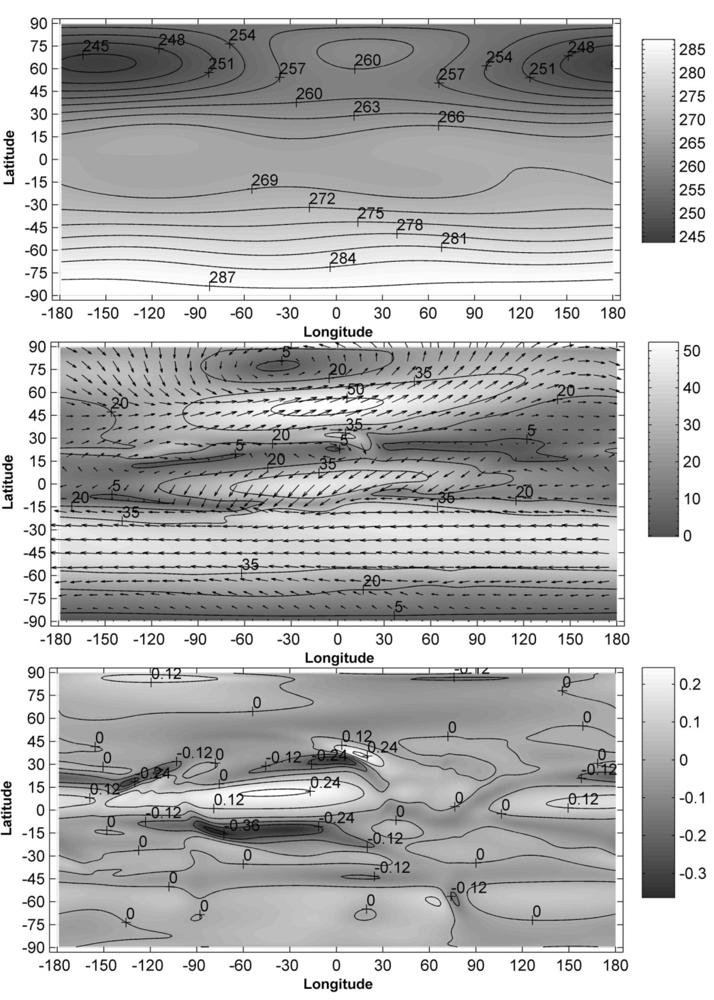
Figure 1. The distributions of the given neutral gas temperature (top panel), vector of the calculated horizontal component of the neutral wind velocity (middle panel), and calculated vertical component of the neutral wind velocity (bottom panel) as functions of longitude and latitude at the altitude of 50 km, obtained for 16 January. The temperature is given in K and wind velocities are given in m/s, with positive direction of the vertical component being upward.

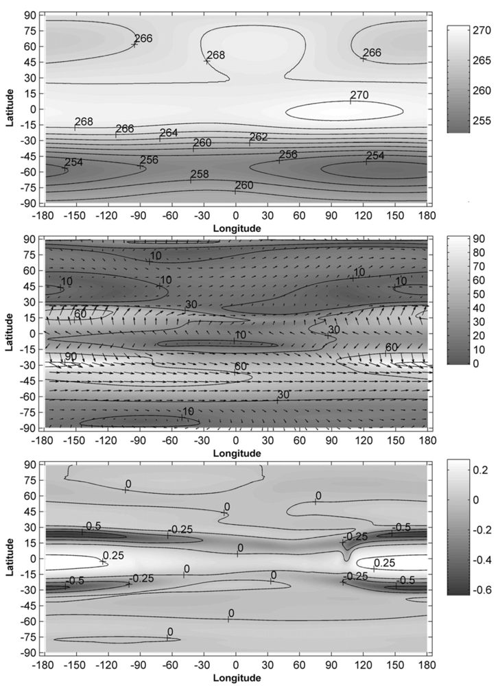
Figure 2. The same as in Figure 1 but obtained for 16 April.

Figure 2. The same as in Figure 1 but obtained for 16 April.

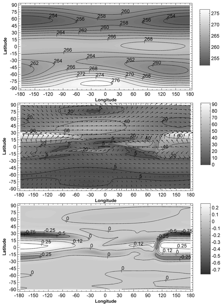
Figure 3. The same as in Figure 1 but obtained for 16 July.

Figure 3. The same as in Figure 1 but obtained for 16 July.

Figure 4. The same as in Figure 1 but obtained for 16 October.

Figure 4. The same as in Figure 1 but obtained for 16 October.

The distributions of the atmospheric parameters corresponding to various seasons, calculated with the help of the mathematical model, illustrate both common characteristic features and distinctions caused by different seasonal conditions.

The calculated global atmospheric circulations possess the following common features: The horizontal component of the wind velocity is a variable function of latitude and longitude at levels of the middle atmosphere; Horizontal domains exist where the steep gradients in the horizontal velocity field take place; The horizontal wind velocity can have various directions which may be opposite at the near points, displaced for a distance of a few steps of finite-difference approximation. Moreover, horizontal domains exist in which the vertical neutral wind component has opposite directions. As a general rule, the horizontal domains, where the vertical neutral wind component is upward, are significantly extended in both latitude and longitude. Contrariwise, horizontal domains having a downward vertical neutral wind component are extended in longitude but narrow in latitude. Usually, the latter domains have a configuration like a long narrow band and coincide, as a rule, with the regions, where the steep gradients in the horizontal velocity field take place. Maximal absolute values of the upward vertical wind component are less than the maximal module of the downward vertical wind component. The horizontal and vertical components of the wind velocity are changeable functions not only of latitude and longitude but also of altitude. The maximum absolute values of the horizontal and vertical components of the wind velocity are larger at higher altitudes. For example, the simulation results have indicated that the downward vertical component of the neutral wind velocity, obtained for 16 January at low latitudes close to a longitude of −120°, achieves a value of −0.24 m/s at the altitude of 50 km (Figure 1). However, this vertical component achieves a value of −3.5 m/s in the same limited horizontal domain at the altitude of 110 km. Similarly, the simulation results have indicated that the vertical component of the neutral wind velocity, obtained for 16 July at low latitudes near a longitude of −120°, achieves a value close to zero (Figure 3). However, this vertical component achieves a value of −5.8 m/s at the same point on globe at an altitude of 110 km. Thus, the vertical wind velocity can achieve values of a few m/s at levels of the lower thermosphere in the horizontal domains having a configuration like a limited narrow band. At levels of the middle atmosphere, the horizontal wind velocity can achieve values of more than 100 m/s.

Let us consider simulation results, obtained for different seasons, and their distinctions. Figure 1 shows the calculated distributions of the horizontal and vertical components of the neutral wind velocity at an altitude of 50 km, obtained on 16 January. Figure 3 shows analogous distributions, obtained on 16 July. These distributions respectively correspond to winter and summer in the northern hemisphere and summer and winter in the southern hemisphere. From Figure 1 one can see that, for winter period in the northern hemisphere, at levels of the middle atmosphere, the horizontal motion of the neutral gas is primarily eastward in the northern hemisphere and primarily westward in the southern hemisphere. Contrariwise, from Figure 3, it is seen that, for the summer period in the northern hemisphere, the directions of these motions are opposite in both hemispheres.

We know that the global atmospheric circulation can sometimes contain so-called circumpolar vortices that are the largest scale inhomogeneities in the global neutral wind system. Their extent can be very large, sometimes reaching latitudes close to the equator. It is well known from numerous observations that circumpolar vortices are formed at heights of the stratosphere and mesosphere in the periods close to summer and winter solstices, when there is no rebuilding of the atmosphere. The circumpolar anticyclone arises in the northern hemisphere under summer conditions, while the circumpolar cyclone arises in the southern hemisphere under winter conditions. Contrariwise, the circumpolar cyclone arises in the northern hemisphere under winter conditions, while the circumpolar anticyclone arises in the southern hemisphere under summer conditions. Let us compare these experimental data with the simulation results, obtained for January and July conditions.

From Figure 1 it can see that a circumpolar cyclone is formed in the winter period in the northern hemisphere (the motion of the neutral gas is primarily eastward), and a circumpolar anticyclone is formed in the summer in the southern hemisphere (the motion of the neutral gas is primarily westward). It can be noticed that the center of the northern cyclone is displaced from the pole by approximately 10° in latitude.

From Figure 3, one can see that a circumpolar anticyclone is formed in the summer period in the northern hemisphere (the motion of the neutral gas is primarily westward), and a circumpolar cyclone is formed in the winter in the southern hemisphere (the motion of the neutral gas is primarily eastward). It is easy to see that the center of the southern cyclone is displaced from the pole by approximately 5° in latitude. It is easy to see that the circumpolar vortices of the northern and southern hemispheres, obtained using the mathematical model at the level of the middle atmosphere for January and July conditions, correspond qualitatively to the global circulation, obtained from observations.

It is clear that the calculated circulations of the middle atmosphere, obtained for January and July dates are completely determined by the horizontal non-uniformity of the neutral gas temperature in the rotating atmosphere.

It is obvious that horizontal non-uniformity of the atmospheric temperature, which is distinct for January and July conditions, significantly influences the formation of the atmospheric circulation at levels of the middle atmosphere, in particular, in the formation of the circumpolar vortices. Incidentally, the qualitative agreement between January and July circulations of the middle atmosphere, obtained numerically and experimentally, manifests the adequacy of the distributions of atmospheric temperature.

The calculated distributions of the horizontal and vertical components of the neutral wind velocity, obtained in the spring period in the northern hemisphere (16 April), are shown in Figure 2. These distributions do not coincide with simulation results, shown neither in Figure 1 (January) nor in Figure 3 (July). However, the horizontal motion of the neutral gas in the northern hemisphere in April is analogous to January circulation (Figure 1). It is seen that the weakened winter circumpolar cyclone continues to exist in the northern hemisphere up to April. Contrariwise, the horizontal motion of the neutral gas in the southern hemisphere in April (Figure 2) is opposite to that obtained during the January conditions (Figure 1). Thus, the January circumpolar anticyclone is destroyed by April in the southern hemisphere. Instead, a circumpolar cyclone arises which continues to exist in the southern hemisphere up to July.

Simulation results, obtained in the autumn period in the northern hemisphere (16 October), are shown in Figure 4. It is easy to see that the primary directions of the neutral gas motions in the northern and southern hemispheres in October are opposite to those obtained for July conditions (Figure 3). It turns out that, until October, the July atmospheric circulation is destroyed in both hemispheres and a new wind system arises which is analogous to the atmospheric flow characteristic in January conditions (Figure 1). The arisen new wind system is enhanced during the period from October to January, especially in the southern hemisphere.

In general, the calculated distribution of the horizontal component of the neutral wind velocity, obtained for 16 April, is a transitional flow from January to July circulation of the middle atmosphere. Similarly, the horizontal flow of the neutral gas, calculated for 16 October, is the transitional motion from July to January atmospheric circulation.

From simulation results, it can be seen that the maximal absolute values of the horizontal component of the wind velocity at a fixed altitude are different for different seasons. These values are the smallest in January. The maximal modules of the vertical wind component at a fixed altitude have distinct values for different seasons, too. The largest values take place in October.

It can be of interest also to compare the simulation results with computational studies of other authors. In the study of Rees et al. [14], the seasonal variations of thermosphere and ionosphere have been numerically investigated using a coupled, three-dimensional, global model. In this study, the calculated parameters have been shown at levels of the E- and F-regions of the ionosphere. The numerical model, utilized in the present study, is intended to investigate the behavior of a neutral gas at levels of the troposphere, stratosphere, mesosphere and lower thermosphere, which are situated at lower altitudes. Therefore, the correct comparison of the simulation results is impossible, unfortunately. In the study of Roble and Ridley [17], a hydrostatic simulation model of the mesosphere, thermosphere and ionosphere with coupled electrodynamics has been applied to calculate the global circulation, temperature and compositional structure between 30 and 500 km for equinox, solar cycle minimum, geomagnetic quiet conditions. The latter conditions do not coincide with the conditions used in the present study, completely. The most appropriate conditions used in the present study are those that were utilized in the calculations for 16 April and 16 October. Comparing the results presented in the study of Roble and Ridley [17] with the results of the present study (Figures 2,4), we can see both common characteristic features and distinctions. The distributions of the horizontal components of the neutral wind velocity calculated by Roble and Ridley [17] for the northern hemisphere are qualitatively similar to results of the present study obtained for 16 October (Figure 4), whereas these results are rather different in the southern hemisphere. The distributions of the horizontal components of the neutral wind velocity calculated by Roble and Ridley [17] for the southern hemisphere are qualitatively similar to results of the present study obtained for 16 April (Figure 2), whereas these results have considerably fewer common features in the northern hemisphere. The differences between the results presented in the study of Roble and Ridley [17] and obtained in the present study are conditioned not only by differences of the input parameters of the models, but also by the distinctions of the utilized mathematical models.

4. Summary and Conclusions

The non-hydrostatic model of the global neutral wind system of the Earth’s atmosphere, developed earlier at PGI, has been applied for simulation of the three-dimensional global distributions of the neutral wind components and neutral gas density for conditions corresponding to four different seasons. The applied mathematical model differs essentially from existing global circulation models of the atmosphere. Firstly, the vertical component of the neutral wind velocity is calculated without using the hydrostatic equation. The vertical component of the neutral wind velocity as well as the horizontal components is obtained by means of a numerical solution of a generalized Navier-Stokes equation for compressible gas, with no single term in this equation being omitted. Secondly, an internal energy equation for the neutral gas is not included in the applied mathematical model. Instead, the global temperature field is assumed to be a given distribution, i.e., the input parameter of the model, and obtained from the NRLMSISE-00 empirical model [26].

By means of our mathematical model, the steady-state distributions were obtained of the atmospheric parameters corresponding to 16 January, 16 April, 16 July and 16 October (all at 10.30 UTC). The calculations were performed at moderate solar activity under low geomagnetic activity conditions.

For all seasons, the horizontal and vertical components of the wind velocity are distinct functions of latitude and longitude at levels of the middle atmosphere. The steep gradients in the horizontal velocity field take place in the horizontal domains having the configuration like a limited narrow band. The horizontal wind velocity can achieve values of more than 100 m/s at levels of the middle atmosphere. The maximal absolute values of the horizontal component of the wind velocity at a fixed altitude are distinct for different seasons. The lowest values are found to exist in January.

The vertical neutral wind velocity can have opposite directions in the horizontal domains having different configurations. Usually, the horizontal domains, where the vertical component of the neutral wind is upward, are similar to a spot having a great length and large width. As a rule, the horizontal domains, where the vertical neutral wind component is downward, are similar to a long narrow band and coincide with the regions where the steep gradients in the horizontal velocity take place. The vertical component of the wind velocity can achieve values of a few m/s at levels of the lower thermosphere in the limited horizontal domains. Doubtless, such values of the vertical wind component are attained due to the non-hydrostatic circulation model, in which the vertical component of the velocity is obtained by means of a numerical solution of the non-simplified momentum equation. The maximal absolute values of the downward vertical wind component exceed those of the upward vertical wind component. The maximal absolute values of the vertical wind velocity at a fixed altitude are distinct for different seasons. The largest values are found in October.

The results of our simulation indicate that the horizontal non-uniformity of the neutral gas temperature, which is distinct in different seasons, considerably affects the formation of the global neutral wind system in the middle atmosphere: in particular, the large-scale circumpolar vortices of the northern and southern hemispheres. It turned out that, in the northern hemisphere, the circumpolar cyclone is formed under winter conditions and the circumpolar anticyclone forms during the summer. In the southern hemisphere, the circumpolar anticyclone is formed in January and the circumpolar cyclone in July. It should be emphasized that the circumpolar vortices of the northern and southern hemispheres, obtained using the mathematical model at levels of the middle atmosphere for January and July conditions, are consistent with existing observational data. Undoubtedly, this fact manifests the adequacy of the atmospheric temperature distributions calculated with the help of the NRLMSISE-00 empirical model [26] and utilized in our numerical simulation.

The simulation results obtained indicate that the calculated distribution of the horizontal component of the neutral wind velocity for April in the northern hemisphere is a transitional flow from January to July circulation of the middle atmosphere. The flow of the neutral gas in the northern hemisphere is analogous to January circulation and the motion in the southern hemisphere is analogous to July circulation.

The simulation results obtained for the autumn period in the northern hemisphere (in October) indicate that the horizontal motion of the neutral gas is the transitional flow from July to January atmospheric circulation. In both hemispheres, the atmospheric circulations at the mesosphere levels are analogous to those for January conditions, with the intensity of the circumpolar vortices of the northern and southern hemispheres in October being less than that in January.

Finally, we note that the non-hydrostatic global circulation model of the middle atmosphere, utilized in the present study, may be applied not only for simulating the dynamic regime of the atmosphere, but also for modeling the behavior of the D region of the ionosphere by taking into account the atmospheric mass motion in the vertical direction, which ought to vary during different seasons. Moreover, the utilized mathematical model of the global wind system of the Earth’s atmosphere has the potential to be applied for numerical simulations of global atmospheric circulations on other planets as well. An example for such an application can be found in [28], where Titan’s atmosphere circulation is simulated.