It is well known that interference exists in IR spectroscopic measurements and causes large uncertainties in observational data if it is not treated properly. Therefore, understanding of IR PAMGA interference is a critical step to ensure accurate air emission monitoring when using such instrumentation.
2.1. IR Spectra of Gas Molecules
Each gas molecule has its own set of characteristic quantum energies. When a molecule absorbs external energy (such as photons in light), it transits from a lower to a higher energy level. When the molecule returns back to its lower energy level, it either emits a photon or releases heat or both. During the transition from one energy level to another, the difference between the higher energy level Ehigh and the lower level Elow of the molecule must be equal to the photon energy (hν) for energy conservation:
where ν is the wavenumber of the photon in cm
−1 and
h is Planck’s constant. Most gas molecules absorb and emit photons in the IR region (ν = 10–14,000 cm
−1), in which the mid-IR region (670–4,000 cm
−1) is widely used in the IR detection of gas molecules. When an IR monochromatic light with single wavenumber enters a chamber that contains a single gas absorbing the light at the same wavenumber, the light intensity decreases after passing through the chamber. The change in light intensity before and after the chamber obeys Beer’s law (e.g., [
21]):
or
where I0 and I are the light intensity before and after passing through the gas chamber at wavenumber ν, ΔI is the absorbed light intensity, L is the length of the chamber along the optical path in meters (m), C is the gas concentration in ppm, and k is the gas absorption coefficients at wavenumber ν in ppm−1∙m−1. I0, I, ΔI, and k are functions of the wavenumber.
The gas concentration inside the chamber can be determined from Equations (2) or (2a) based on the change in light intensity, when the absorption coefficient
k(
ν) and optical length
L are known. The absorption coefficients of many molecules have been determined in previous work and can be found in many databases (e.g., [
22,
23]). If the photon energy does not match the energy difference between the higher and lower energy levels, the molecule does not absorb the light at this wavenumber,
i.e., the absorption coefficient
k(
ν) is zero, and therefore the light intensity remains unchanged,
i.e.,
I(
ν) =
I0(
ν) or
ΔI(
ν) = 0. When a light covering a wide IR spectral range passes through a chamber with a single gas inside, the changes in light intensity will be the function of the wavenumber, which is referred to as the IR spectrum of the gas.
When the gas absorption is small (i.e., k(ν)CL << 1), the absorbed light intensity is linearly proportional to the gas concentration C:
Simplification from Equation (2a) to (2b) is reasonable as long as the gas concentrations are in the linear measurement range because the IR gas analyzers provide a linear response to the gas concentrations. When an IR light intensity is modulated at an “audio” frequency, the heat released by the molecule when transiting from a higher to a lower energy level produces a sound signal at the same frequency inside the chamber that can be detected by microphones. Intensity of the microphone signal is proportional to the absorbed light intensity
ΔI(
ν) [
18]. The change in microphone signal with the light wavenumber is referred to as the IR photoacoustic spectrum of the gas.
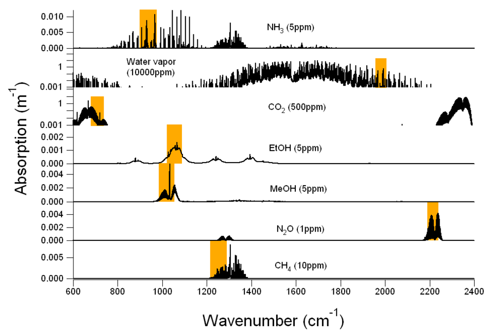
Figure 1 shows the IR absorption spectra of CH
4, CO
2, MeOH, EtOH, N
2O, NH
3 and H
2O in the IR region of 600–2,400 cm
−1. The IR spectral data of these molecules were obtained from the IR spectral library of the Pacific Northwest National Laboratory [
23] in 0.1 cm
−1 resolution. Each gas molecule has its characteristic spectrum in terms of wavenumber region, absorption intensity, and structure (
Figure 1), by which the gas can be identified and quantitatively detected. However, because every gas molecule has a set of characteristic IR spectra, the IR spectra of several gas molecules may overlap in a particular IR spectral region and therefore these gas molecules absorb light at the same wavenumber. Overlaps of the gas IR spectra can be seen in
Figure 1.
Figure 1.
Example of infrared (IR) absorption spectra of CH4, CO2, MeOH, EtOH, N2O, NH3 and H2O (black solid lines). Locations and bandpass of filters corresponding to each gas are shown in orange rectangles on each plot. In Example #1, CH4, CO2, MeOH, EtOH, N2O and H2O are target gases and NH3 is the non-target gas. In Example #2, CO2, MeOH, EtOH, N2O, NH3 and H2O are target gases and CH4 is the non-target gas.
If there are multiple gases inside the chamber and some of them absorb light at the same wavenumber ν, the transmitted light intensity becomes:
where N is the number of gas molecules that absorb light at wavenumber ν. The absorbed light intensity becomes:
When the gas absorption is small (k(ν)CL << 1), the absorbed light intensity is:
It is almost impossible to derive gas concentrations from Equations (3)–(3b) at a single IR wavenumber because the change in IR light intensity is due to absorption by several gases, but it may be possible to do so in multiple IR regions. For example, the Innova 1412 (AirTech Instruments, Ballerup, Denmark), an IR PAMGA, uses up to six filters to select IR light in up to six spectral regions to detect up to six gases sequentially. Because there are multiple gases in the monitoring environment in this case, overlaps of gas IR spectra may cause interference in gas detection and therefore may introduce measurement errors if the interference is not properly treated.
2.2. Estimation of the Interference by IR Spectroscopic Analysis (IRSA)
Because the IR PAMGA employs an IR spectroscopic technique to measure multiple gases, interference between the gases is likely to occur due to the overlaps of IR spectra. In order to reduce the interference, the first step is to properly configure the filters in IR PAMGA based on the IR absorption of all gases of interest in the monitoring environment. In the present study, two filter configurations were used as examples and are listed in
Table 1, which includes channels, filter names, target gases, central, starting, and ending wavenumbers of the bandpass filters. In Example #1, six filters were selected to monitor target gases of MeOH, EtOH, N
2O, CO
2, CH
4 and H
2O in channels A, B, C, D, E, and W, respectively. In Example #2, the target gases were MeOH, EtOH, N
2O, CO
2, NH
3 and H
2O in channels A, B, C, D, E, and W, respectively. The IR absorption spectra of these gases are shown in
Figure 1 (black thick lines) together with the locations and bandpass of the corresponding filters (orange rectangles). Filter names and their paired target gases are presented in
Table 1. Concentrations of the target gases in
Figure 1 were 10 ppm for CH
4, 5 ppm for MeOH, EtOH, and NH
3, 1 ppm for N
2O, 500 ppm for CO
2, and 10,000 ppm for H
2O. Because of the wide range in agricultural air emissions from very low (ppb level) in open sources to extremely high (thousands ppm level) in the enclosed animal housing, the vertical scale of the IR spectra in
Figure 1 would change with the real concentrations, but the locations and bandpass of filters would not. According to
Table 1 and
Figure 1, the six gas/filter combinations in Example #1 corresponded to the six plots from the second to the seventh in
Figure 1, and the six gas/filter combinations in Example #2 to those from the first to the sixth in
Figure 1. The vertical-axis is a log scale for CO
2 and H
2O and linear for other gases.
First, the selected filters must be located in the absorption regions of their target gases, away from the strong absorption for high concentration gases, and close to the central peak for low concentration gases.
Figure 1 shows that the H
2O filter was located at the far wings of a water vapor absorption band to avoid saturation caused by strong absorption near the band center. The CO
2 filter was located at a weak absorption band to avoid saturation as well. For other target gases, the filters were located near the band center to achieve stronger absorption.
Table 1.
Filter configurations and filter/target gas combinations in Example #1 and #2.
Table 1.
Filter configurations and filter/target gas combinations in Example #1 and #2.
| Channel in Example #1 | Channel in Example #2 | Filter Name | Target Gas | Filter Center (cm−1) | FilterBandpass (cm−1) |
|---|
| A | A | UA 0936 | MeOH | 1,020 | 989–1,053 | |
| B | B | UA 0974 | EtOH | 1,061 | 1,027–1,096 | |
| C | C | UA 0985 | N2O | 2,215 | 2,193–2,237 | |
| D | D | UA 0982 | CO2 | 710 | 683–737 | |
| E | - | UA 0969 | CH4 | 1,254 | 1,220–1,289 | |
| - | E | UA 0976 | NH3 | 941 | 908–974 | |
| W | W | SB 0527 | H2O | 1,985 | 1,965–2,205 | |
Secondly, the selected filters should be located at the spectral regions where overlaps between the IR spectra are as few as possible because spectra overlaps would cause interference in multiple gas measurements. The overlaps between the gas IR spectra can be easily identified by aligning the IR spectra of all gases in one graph.
Figure 1 shows the NH
3 interference at the MeOH and EtOH filters, the MeOH interference at the EtOH filter, and the EtOH interference at the MeOH filter. By contrast, the CH
4 interference on other gases is not likely to occur because the CH
4 absorption band is located far away from other filters. Because the IR spectra of water vapor cover a wide spectral range, water vapor interferes with most gases unless the air sample is dry. Therefore, a H
2O filter must be included in the filter configuration when the PAMGA is used in atmospheric applications. In
Table 1, the H
2O filter was installed in channel W for both Examples #1 and #2. Although
Figure 1 only represents the IR spectra of the selected filter configuration at the selected concentrations of their target gases, the procedure to examine the overlaps of gas IR spectra can be applied to any filter configuration at any gas concentration. Since it is not practical to produce graphs similar to
Figure 1 for every filter configuration and every gas concentration in one presentation, users of the IR PAMGA can make similar graphs for the filter configurations and gas concentrations of interest to perform the IRSA. To study the interference between multiple gases at variable concentrations, gas absorption coefficients are more frequently used as described below.
In order to quantitatively compare the absorption of the selected gases at an IR PAMGA filter, absorption coefficients measured at the standard ambient pressure and temperature of 101.3 kPa and 25 °C by the PNNL [
23] were used to derive the total absorption of the gases at that particular bandpass. The total absorption (m
−1) of a gas at a filter bandpass was an integration of individual absorption coefficients from the PNNL database over the entire filter bandpass and then multiplied by the gas concentration.
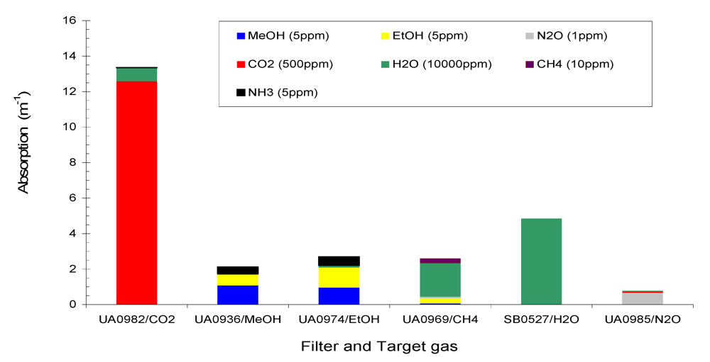
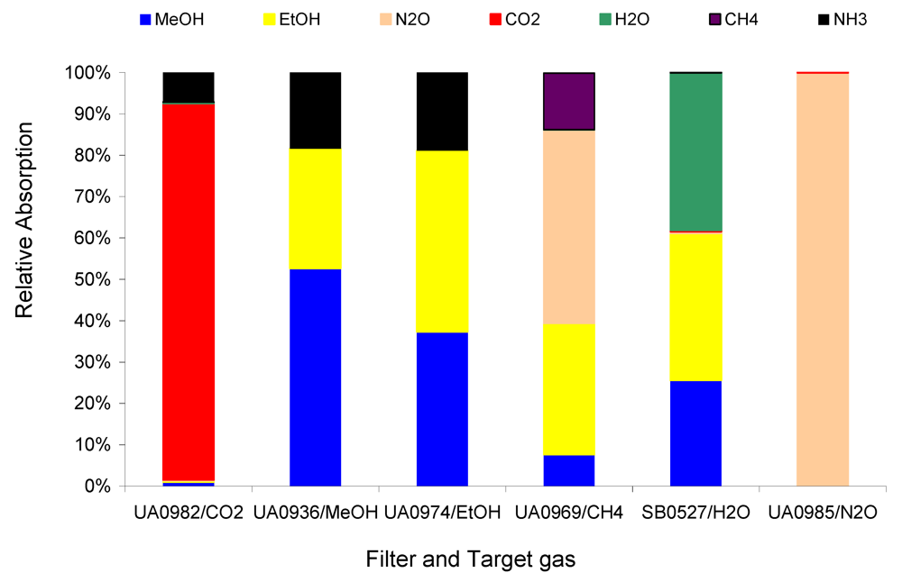
Figure 2 shows the total absorption of the six target gases CH
4 (10 ppm), MeOH (5 ppm), EtOH (5 ppm), N
2O (1 ppm), CO
2 (500 ppm), H
2O (10,000 ppm) and a non-target gas NH
3 (5 ppm) at the six filters of Example #1.
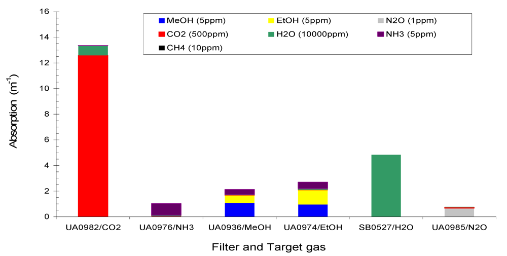
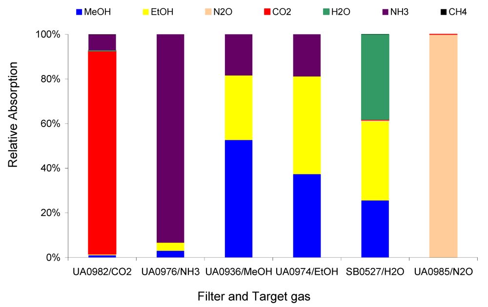
Figure 3 shows the total absorption of the six target gases NH
3 (5 ppm), MeOH (5 ppm), EtOH (5 ppm), N
2O (1 ppm), CO
2 (500 ppm), H
2O (10,000 ppm), and a non-target gas CH
4 (10 ppm) at the six filters of the Example #2. It is seen in
Figure 2 and
Figure 3 that (1) total absorption at a given filter consisted of contributions from several gases due to the overlaps of IR spectra at that filter; (2) one gas contributed to several filters, and (3) non-target gases made contributions to several filters. Therefore, interference between the gases in IR PAMGA measurements would most likely occur. In order to separate the contributions of multiple gases in multiple filters and reduce the interference, mathematical algorithms are needed. The algebraic matrix method may be a good choice for this purpose because it can mathematically solve this kind of problem. Before introducing the algebraic matrix, we will continue to discuss the interference in IR PAMGA measurements based on gas IR spectra.
Figure 2.
Absorption of Example #1 target gases (CH4 = 10 ppm, CO2 = 500 ppm, MeOH = 5 ppm, EtOH = 5 ppm, N2O = 1 ppm, and H2O = 10,000 ppm) and non-target gas (NH3 = 5 ppm) at each filter.
Figure 2.
Absorption of Example #1 target gases (CH4 = 10 ppm, CO2 = 500 ppm, MeOH = 5 ppm, EtOH = 5 ppm, N2O = 1 ppm, and H2O = 10,000 ppm) and non-target gas (NH3 = 5 ppm) at each filter.
Figure 3.
Absorption of Example #2 target gases (NH3 = 5 ppm, CO2 = 500 ppm, MeOH = 5 ppm, EtOH = 5 ppm, N2O = 1 ppm, and H2O = 10,000 ppm) and non-target gas (CH4 = 10 ppm) at each filter.
Figure 3.
Absorption of Example #2 target gases (NH3 = 5 ppm, CO2 = 500 ppm, MeOH = 5 ppm, EtOH = 5 ppm, N2O = 1 ppm, and H2O = 10,000 ppm) and non-target gas (CH4 = 10 ppm) at each filter.
Figures 2 and 3 were produced for selected filter configurations and gas concentrations to show the possible interference between these gases. Similar plots can be made for different filter configurations at various gas concentrations after the total absorption at each filter are computed from the PNNL IR spectral database. Because gas concentrations vary in the real world, it is impossible to make graphs for every gas concentration to perform the IRSA. It would be better to have a single plot or table for a given filter configuration which can be used for IRSA at variable gas concentrations. For this purpose, total absorptions of these gases at a concentration of 1 ppm are provided in
Table 2.
Figure 4 compares the relative absorptions of the 1 ppm target gases CH
4, MeOH, EtOH, N
2O, CO
2, and H
2O in Example #1 with the introduction of 1 ppm non-target gas NH
3.
Figure 5 shows the comparison between 1 ppm target gases NH
3, MeOH, EtOH, N
2O, CO
2, and H
2O in Example #2 with the introduction of 1 ppm non-target gas CH
4.
Figure 4 depicts the strong interference of the non-target gas NH
3 on the target gases MeOH and EtOH, less interference on CH
4 and CO
2, and much less interference on N
2O. The relative absorption shown in
Figure 4 and
Figure 5 indicate the relative interference of the non-target on the target gases. The relative interference of 1 ppm non-target gas NH
3 on 1 ppm target gases MeOH, EtOH, N
2O, CO
2, and CH
4 are 349, 432, 0, 78, and 11 ppb per ppm NH
3, respectively, which were derived from
Table 2. These relative interference values can be used to determine the interference of a non-target gas at any concentration, e.g., 10 ppm NH
3 could cause about 3.5, 4.3, 0, 0.8, and 0.1 ppm interference, respectively, in the measurements of MeOH, EtOH, N
2O, CO
2, and CH
4. Either the relative absorption in
Figure 4 or the calculated relative interference in
Table 2 can inform the user of how the non-target gas would directly affect the measurements of the target gases if the non-target gas exists. Obviously, the Example #1 cannot be used in applications where NH
3 appears to be at elevated concentrations.
As another example, the IRSA was applied to
Figure 5. The relative interference of 1 ppm non-target gas CH
4 on 1 ppm target gases NH
3, MeOH, EtOH, N
2O, and CO
2 in Example #2 were hardly observed in
Figure 5 but can be derived from
Table 2. They were 11, 12, 21, 4, and 362 ppt per ppm CH
4, respectively, therefore can be neglected when the CH
4 concentration is low. When CH
4 was as high as 1,000 ppm, the errors caused directly by CH
4 would be 11, 12, 21, 4, and 362 ppb, respectively, in the NH
3, MeOH, EtOH, N
2O and CO
2 measurements. So, the CH
4 interference in Example #2 was still negligible even if the CH
4 was up to thousands of ppm, while the target gases were at a few ppm.
Figure 4.
Relative absorption of 1 ppm non-target NH3 and 1 ppm target gases at each filter in Example #1.
Figure 4.
Relative absorption of 1 ppm non-target NH3 and 1 ppm target gases at each filter in Example #1.
Figure 5.
Relative absorption of 1 ppm non-target CH4 and 1ppm target gases at each filter in Example #2.
Figure 5.
Relative absorption of 1 ppm non-target CH4 and 1ppm target gases at each filter in Example #2.
Table 2.
Total absorption of 1 ppm gas at each filter, NH3 relative interferenceon target gases in Examples #1, and CH4 relative interference on target gases in Example #2.
Table 2.
Total absorption of 1 ppm gas at each filter, NH3 relative interferenceon target gases in Examples #1, and CH4 relative interference on target gases in Example #2.
| Filter | Total Absorption of 1 ppm Gas (m−1) | NH3 RIF*ppbper ppm | CH4 RIF *pptper pm |
|---|
| MeOH | EtOH | N2O | CO2 | CH4 | H2O | NH3 |
|---|
| MeOH | 2.2 × 10⁻¹ | 1.2 × 10⁻¹ | 5.0 × 10⁻⁶ | 1.5 × 10⁻⁵ | 2.6 × 10⁻⁶ | 5.2 × 10⁻⁶ | 7.6 × 10⁻² | 349 | 12 |
| EtOH | 1.9 × 10⁻¹ | 2.3 × 10⁻¹ | 1.3 × 10⁻⁵ | 3.2 × 10⁻⁵ | 4.7 × 10⁻⁶ | 9.8 × 10⁻⁶ | 9.8 × 10⁻² | 432 | 21 |
| N2O | 3.9 × 10⁻⁴ | 5.4 × 10⁻⁴ | 6.6 × 10⁻¹ | 1.4 × 10⁻⁴ | 2.5 × 10⁻⁶ | 4.0 × 10⁻⁶ | 2.6 × 10⁻⁶ | 4 × 10⁻³ | 4 |
| CO2 | 2.7 × 10⁻⁴ | 9.3 × 10⁻⁵ | 4.9 × 10⁻⁵ | 2.5 × 10⁻² | 9.1 × 10⁻⁶ | 7.6 × 10⁻⁵ | 2.0 × 10⁻³ | 78 | 362 |
| CH4 | 1.4 × 10⁻² | 5.8 × 10⁻² | 8.5 × 10⁻² | 8.0 × 10⁻⁶ | 2.5 × 10⁻² | 1.9 × 10⁻⁴ | 2.9 × 10⁻⁴ | 11 | - |
| H2O | 3.2 × 10⁻⁴ | 4.5 × 10⁻⁴ | 5.6 × 10⁻⁶ | 4.3 × 10⁻⁶ | 7.3 × 10⁻⁷ | 4.8 × 10⁻⁴ | 3.8 × 10⁻⁹ | 8 × 10⁻³ | 1517 |
| NH3 | 5.8 × 10⁻³ | 6.9 × 10⁻³ | 2.2 × 10⁻⁵ | 1.1 × 10⁻⁵ | 1.9 × 10⁻⁶ | 6.0 × 10⁻⁶ | 1.8 × 10⁻¹ | - | 11 |
2.3. Experimental Tests on the Interference
In order to validate the IRSA method, experimental tests were conducted at California Analytical Instruments, Inc (CAI) using an Innova 1412 analyzer with two configurations as shown in
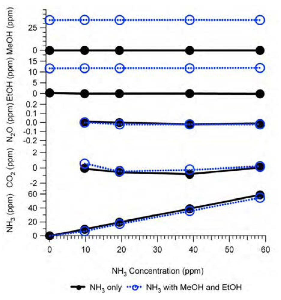
Table 1. First, the analyzer was fully calibrated by CAI because it is a manufacturer authorized calibration facility. The NH
3 interferences as a non-target gas in Example #1 (because the NH
3 filter was not installed) are shown in
Figure 6 and as a target gas in Example #2 (because the NH
3 filter was installed) are shown in
Figure 7.
Figure 6.
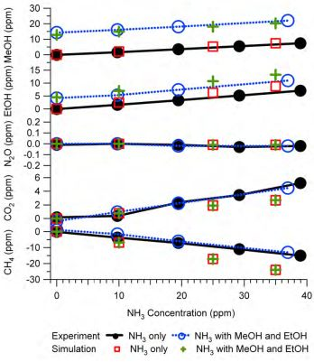
Interference of NH3 in Example #1 as a non-target gas. Black solid lines with closed circles are experimental responses to NH3 only (NH3 = variable, other gases = 0 ppm), blue dash lines with open circles are experimental responses to NH3 in the presence of MeOH (12.8 ppm) and EtOH (4.5 ppm), and red thin-lines with crosses are estimation by the IRSA method for the NH3 only test. All gas mixtures were in N2 balance and not humidified.
Figure 6.
Interference of NH3 in Example #1 as a non-target gas. Black solid lines with closed circles are experimental responses to NH3 only (NH3 = variable, other gases = 0 ppm), blue dash lines with open circles are experimental responses to NH3 in the presence of MeOH (12.8 ppm) and EtOH (4.5 ppm), and red thin-lines with crosses are estimation by the IRSA method for the NH3 only test. All gas mixtures were in N2 balance and not humidified.
Figure 7.
Interference of NH3 in Example #2 as a target gas. Black solid lines with closed circles are experimental responses to NH3 only (NH3 = variable and other gases = 0 ppm) and blue dash lines with open circles are experimental responses to NH3 in the presence of MeOH (35.2 ppm) and EtOH (12.2 ppm). All gas mixtures were in N2 balance and not humidified. Analytical results of the interference of NH3 as a target gas were not available because the IRSA method is used to estimate the interference of non-target gases.
There are two tests shown in
Figure 6: (1) the non-target gas NH
3 only was fed to the analyzer in various concentrations while all target gas concentrations were zero and (2) the non-target gas NH
3 was mixed with MeOH (12.8 ppm) and EtOH (4.5 ppm) in various concentrations before the mixture was fed to the analyzer while the other gas concentrations were zero. Experiment (1) was titled the “NH
3 only test” and experiment (2) the “tri-gas test”, which was the simplest case of a multi-gas test. In both experiments, the sample gases were obtained from standard gas cylinders in N
2 balance and were not humidified (H
2O = 0 ppm). The analyzer’s internal cross compensation algorithm was used in both experiments. The interference of non-target gas NH
3 on target gases MeOH, EtOH, N
2O, CO
2, and CH
4 were calculated based on the relative interference given in
Table 2 at various NH
3 concentrations in the absence of other gases (NH
3 only test). The IRSA results are also shown in
Figure 6. The experimental results in
Figure 6 indicate that the NH
3 interference as non-target gas on the IR PAMGA measurements seem independent of the target gas concentrations because the line slopes in each graph are very close between the NH
3 only and tri-gas tests.
Figure 6 reveals that the interference of non-target gases cannot be addressed by the analyzer’s internal cross compensation algorithm.
Comparisons between the experimental results and IRSA results in
Figure 6 show a good agreement for N
2O and an overestimation for MeOH and EtOH. However, the negative interference of the non-target gas NH
3 on the target gas CH
4 measurements in
Figure 6 was not predicted by the IRSA method. Because there was no direct overlapping spectra between NH
3 and CH
4 at the CH
4 filter, NH
3 did not directly interfere with CH
4 (primary interference), but NH
3 had a secondary interference on CH
4,
i.e., NH
3 had a primary interference on EtOH at the EtOH filter and in turn EtOH had a primary interference on CH
4 at the CH
4 filter. The similar secondary inference of NH
3 on CH
4 via MeOH also happened due to the same procedure. It may be difficult to understand the negative interference of NH
3 on CH
4 as shown in
Figure 6, but an explanation is provided below based on gas IR spectra as shown in
Figure 1. The non-target gas NH
3 in Example #1 absorbed light at both MeOH and EtOH filters (Figures 1, 2, and 4) contributing a positive artifact in both MeOH and EtOH measurements. This positive artifact was then transferred to the CH
4 filter because MeOH and EtOH absorbed light at the CH
4 filter. In order to compensate for these positive artifacts at the CH
4 filter, the analyzer erroneously deduced a negative concentration of CH
4 through the internal cross compensation procedure. Because the IRSA method did not involve any cross compensation, it could not predict the secondary interference. Therefore, an algebraic matrix calculation is needed to estimate both primary and secondary interference, which will be discussed in
Section 2.4.
The “NH
3 only” and “tri-gas” experiments were also conducted using the Example #2 analyzer, except that the NH
3 was a target gas because the NH
3 filter was installed in Example #2, and the results are shown in
Figure 7.
Figure 7 reveals that the interference of the target gas NH
3 on MeOH and EtOH was eliminated by the analyzer’s built-in cross compensation algorithm. No IRSA was performed for the NH
3 interference as a target gas because the IRSA method can only estimate the interference of non-target gases. Again, in order to simulate the interference of both target gas and non-target gas, an algebraic matrix is needed as described in
Section 2.4.
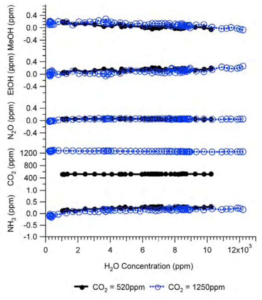
Because the IR spectrum of water vapor covers a wide spectral range and overlaps with that of many other gases, water vapor is a very important gas in terms of interference with other gas measurements. Therefore, water vapor must be measured as a target gas. This means that a H
2O filter must be included in the filter configuration. The interference of water vapor as a target gas in Example #2 was experimentally tested and the results are shown in
Figure 8. The CO
2 gas at a constant concentration was humidified before entering the IR PAMGA using Nafion tubing over a heated water bath. The concentration of water vapor was adjusted by changing the water bath temperature. Two concentrations of CO
2 at 520 ppm and 1,250 ppm in ultra-zero air were used respectively in the tests, while all other gases were 0 ppm.
Figure 8 reveals that the interference of water vapor as a target gas was also eliminated by the analyzer’s internal across compensation algorithm because changes in the measured concentrations of other target gases were almost independent of the water vapor concentrations.
Figure 8.
Interference of H2O in Example #2 as a target gas. Black solid lines with closed circles are experimental responses to 520 ppm CO2 and blue dashed lines with open circles are experimental responses to 1,250 ppm CO2. All other gases were 0 ppm. Analytical results of the interference of H2O as a target gas were not available because the IRSA method is used to estimate the interference of non-target gases.
2.4. Mathematical Simulation of the Interference
As discussed in
Section 2.3 the internal cross compensation method of IR PAMGA can eliminate the interference between target gases but cannot address the interference of non-target gases. The IRSA method can be used to estimate the primary interference of non-target gases but cannot predict the secondary interference. Therefore, another approach is needed to address all of these issues. Because the interference in IR PAMGA occurred between multi-gases cross multiple filters, an algebraic matrix calculation would be a good method to solve the problem.
Assuming that six filters were installed in the IR PAMGA to measure six target gases including H2O, Si represents the microphone signal in μV from filter i (i = 1, 2, …, 6), Cj is the concentration in ppm of target gas j (j = 1, 2, …, 6), and αi,j is the contribution of target gas j to the microphone signal Si. The αi,j is referred to as sensitivity coefficient in μV/ppm. Because of the overlaps of gas IR spectra, αi≠j may not be zero, the target gas j would contribute to microphone signal Si (i ≠ j) and cause interference on the measurement of the target gas i. In theory, the microphone signal Si of IR PAMGA can be expressed as functions of the target gas concentrations Cj:
These linear algebraic Equations can also be expressed with an algebraic matrix Equation:
or simply
where both [Si] and [Ci] are a 1 × 6 matrix and [αi,j] a 6 × 6 matrix, respectively. Equation (4b) can be solved using an algebraic matrix Equation.
where matrix [αi,j]−1 is the inverse of the matrix [αi,j]. Because the method to calculate Equation (4c) can be found in any textbook of linear algebraic theory, it is not described here. In addition, there are many software packages with built-in programs to solve such linear algebra problems, so it is straightforward to calculate the variables [Ci] when microphone signals [Si] and sensitivity coefficients [αi,j] are known. The sensitivity coefficients [αi,j] can be obtained by calibrating the IR PAMGA. Although six filters were assumed to derive Equations (4a)–(4c), the Equations can be applied to any number of filters in the PAMGA.
In order to introduce the interference of non-target gases, Equation (4) can also be expressed as:
In the real monitoring environments, there may be other gases as well as random electronic noise that, in addition to the target gases, contribute to the microphone signals. Considering all these factors, Equation (5) becomes
where, φi is the total contribution of all non-target gases to the microphone signal Si and Ei is the electronic noise (zero offset) at filter i. It is obvious that, for the same microphone signals Si (i = 1, 2, 3,…6), the solutions Cj would be different between Equations (5) and (5a) if non-target gases and electronic noise exist (φi≠0 and Ei≠0). The differences in solution Cj between Equations (5) and (5b) are errors caused by non-target gas interference φi and noise Ei. In general, when the interference and electronic noise increase, the difference in solution between Equations (5a) and (5) also increases and therefore the uncertainty of the IR PAMGA measurements increases. There are several ways to reduce measurement errors. One is to decrease the electronic noise Ei by increasing the measurement interval. As mentioned in previous sections, properly configuring the filters in IR PAMGA based on the presence of all possible gases and their IR absorption properties is a key procedure to reduce the contribution of the non-target gas interference φi.
When the sensitivity coefficients α
i,j are available after calibration, the interference between the target gases can be simulated by solving Equation (5). It is also possible to evaluate the interference of non-target gases on IR PAMGA measurements by solving Equation (5a) when the non-target gases have also been calibrated. In some cases, when the calibrated sensitivity coefficients are not available, a simulation of the interference may be needed to assess its effect in the IR PAMGA measurements. Next we will discuss this possibility. Because the microphone signal of a single gas is proportional to the absorbed light intensity [
18], it can be expressed as:
where β is a factor that includes the combined effects of temperature, pressure, thermal property of gases in the gas chamber, and geometry of the gas chamber,
etc. [
18]. Using Equation (3a), Equation (6) can be expressed as:
Or using Equation (3b) when gas absorption is low, Equation (6) becomes:
or:
Now, it can be seen that Equation (6c) is similar to the algebraic matrix Equation (5). Defining Si' = Si/βI0L (m−1) as simulation signal, the simulation signals at the six filters in IR PAMGA are:
Equation (7) is also an algebraic matrix Equation similar to Equation (5). Thus, variables
Cj can be solved from Equations (7) only if the simulation signals are known because absorption coefficients can be computed from available databases [
23]. For mathematical simulation purposes, we may be able to use gas absorption coefficients
ki,
j instead of sensitivity coefficients α
i,
j, using the simulation signal S
i' instead of the microphone signal
Si to simulate the interference in IR PAMGA.
If we only consider the interference of one non-target gas without electronic noise (Ei = 0), then Equation (5a) becomes:
where kin and Cn are the absorption coefficient at filter i and the concentration of the non-target gas, respectively. From Equations (7) and (7a), the interference of the non-target gas in IR PAMGA measurements can be mathematically estimated based on the selected filters and the IR absorption coefficients of all gases in the monitoring environment without calibrating the analyzer. This method might prove beneficial for IR PAMGA users when planning a new filter configuration for their analyzers. The procedure to simulate the interference using Equations (7) and (7a) is described below:
Use initial concentrations of the target gas CiI and their absorption coefficients ki,j to calculate initial simulation signals SiI using Equation (7), where superscript “I” represent initial values.
Add non-target gas absorption kinCn in Equation (7a).
Subtract kinCn from the initial signals SiI to produce disturbed signals Sid, where superscript “d” represents disturbed values.
Solve Equation (7) again using ki,j and Sid to obtain disturbed target gas concentrations Cid.
The differences in target gas concentrations between initial CiI and disturbed Cid values reveal the interference of the non-target gas in IR PAMGA measurements.
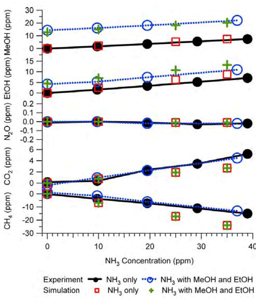
Figure 9 is an example of the simulation results and their comparison with the experimental tests. The experiments were the same as those described in
Figure 6, therefore
Figure 9 is similar to
Figure 6 except that the NH
3 interference on IR PAMGA measurements was assessed by the mathematical simulation using Equations (7) and (7a) instead of the IRSA method. The NH
3 interference on target gases is almost independent of the target gas concentrations because the changes in interference with the NH
3 concentrations (line slopes) were very similar between the NH
3 only (NH
3 = variable and other gases = 0 ppm) and the tri-gas (MeOH = 12.8 ppm, EtOH = 4.5 ppm, NH
3 = variable, and other gases = 0 ppm) tests. Actually, the simulation was also conducted for multiple target gases at various concentrations in addition to the tri-gas (MeOH, EtOH and NH
3) in
Figure 9 and the conclusion remained the same (not shown in any Figures because no experimental comparison was made).
Table 3 compares the NH
3 relative interference (ppb per ppm NH
3) on target gases in Example #1 as a non-target gas. The relative interferences in
Table 3 were obtained by IRSA, mathematical simulation, and experiments, respectively.
Table 3.
Comparison of NH3 relative interference on target gases in Example #1 as a non-target gas (ppb per ppm NH3).
Table 3.
Comparison of NH3 relative interference on target gases in Example #1 as a non-target gas (ppb per ppm NH3).
| Target Gas | IRSA | Mathematical Simulation | Experiment (NH3 Only) | Experiment (Tri-Gas) |
|---|
| MeOH | 349 | 212 | 182 ± 10 | 215 ± 42 |
| EtOH | 432 | 250 | 174 ± 8 | 172 ± 58 |
| N2O | 0.004 | −0.4 | 0 ± 0.3 | 0 ± 0.4 |
| CO2 | 78 | 76 | 103 ± 42 | 122 ± 28 |
| CH4 | 11 | −686 | −377 ± 9 | −302 ± 145 |
Figure 9.
Interference of NH3 on target gases in Example #1 as a non-target gas. Black solid lines with closed circles are experimental responses to NH3 only (NH3 = variable, other gases = 0 ppm), blue dash lines with open circles are experimental responses to NH3 in the presence of MeOH (12.8 ppm) and EtOH (4.5 ppm), red squares are results of mathematical simulation for the NH3 only test, and green crosses are simulation for the tri-gas test. All gas mixtures were in N2 balance and not humidified.
The agreement between predictions and experiments for MeOH and EtOH were improved significantly by the mathematical simulation in comparison with the IRSA results (Figures 6 and 9 and
Table 3). The NH
3 relative interferences on N
2O and CO
2 predicted by both IRSA and mathematical simulation were similar. They agreed well with experiments for N
2O (almost zero), but the prediction was lower than the experimental results for CO
2. The negative effect of the NH
3 interference on CH
4 measurements was successfully predicted by the mathematical simulation, which was due to the secondary interference but could not be predicted by the IRSA method (Figures 6 and 9 and
Table 3). The difference between measurements and simulations might be due to the zero offset
Ei in the IR PAMGA which was ignored in the simplified Equation (7a). The rectangle simplification of the filter bandpass shape may result in some difference in calculating the absorption coefficients and therefore cause simulating errors in Equations (7) and (7a). The dependence of microphone signals on temperature and pressure was ignored when the sensitivity coefficients α
i,
j in Equations (5) and (5a) were replaced with gas IR absorption coefficients
ki,
j in Equations (7) and (7a) and the simulation signal
Si' was used, which might cause some simulation errors. The simulation accuracy could be improved if all target and non-target gases were calibrated and the calibration data were used in the mathematical simulation. But the calibration data of non-target gases were usually not available because the manufacturers rarely provided this information. This is one of the reasons why the gas absorption coefficients were used in this study instead of the calibration data to simulate the interference. Although both IRSA and mathematical simulation methods are not ready yet for use to correct the errors caused by the interference of non-target gases because of their accuracy, they still can be used to select filters, simulate the interference of non-target gases, and therefore would be helpful for properly using the IR PANGA. A significant advantage is that the two methods can be performed prior to the instrument calibration, which would be very convenient for IR PAMGA users.
The simulations of CH4 interference in the Example #2 measurements as a non-target gas were also conducted at various target gas concentrations. It was predicted by the IRSA that the CH4 interferences in the Example #2 measurements were nearly zero at all 6 filters because the absorption of CH4 at any of these filters was almost zero. The mathematical simulation using Equations (7) and (7a) came to the same conclusion.


