Modeling Multiple-Core Updraft Plume Rise for an Aerial Ignition Prescribed Burn by Coupling Daysmoke with a Cellular Automata Fire Model

Abstract

Smoke plume rise is critically dependent on plume updraft structure. Smoke plumes from landscape burns (forest and agricultural burns) are typically structured into “sub-plumes” or multiple-core updrafts with the number of updraft cores depending on characteristics of the landscape, fire, fuels, and weather. The number of updraft cores determines the efficiency of vertical transport of heat and particulate matter and therefore plume rise. Daysmoke, an empirical-stochastic plume rise model designed for simulating wildland fire plumes, requires updraft core number as an input. In this study, updraft core number was gained via a cellular automata fire model applied to an aerial ignition prescribed burn conducted at Eglin AFB on 6 February 2011. Typically four updraft cores were simulated in agreement with a photo-image of the plume showing three/four distinct sub-plumes. Other Daysmoke input variables were calculated including maximum initial updraft core diameter, updraft core vertical velocity, and relative emissions production. Daysmoke simulated a vertical tower that mushroomed 1,000 m above the mixing height. Plume rise was validated by ceilometer. Simulations with two temperature profiles found 89–93 percent of the PM_2.5 released during the flaming phase was transported into the free atmosphere above the mixing layer. The minimal ground-level smoke concentrations were verified by a small network of particulate samplers. Implications of these results for inclusion of wildland fire smoke in air quality models are discussed.

1. Introduction

Approximately six million acres (2.4 million ha) of forest and agricultural land are burned each year in the southern United States to accomplish a number of land management objectives [1]. Most of this burning is accomplished during winter and early spring during days considered favorable for burning. Forestry smoke contributes significantly to the budget of particulate matter in the atmosphere and poses a threat—either as a nuisance, visibility, or transportation hazard [2,3], and/or as a health hazard [4]. The hazard can be local and/or regional depending on the area of the region subjected to burning, the amount of fuel burned, and the number of prescribed burns being conducted on a given day.

Biomass burning is the dominant source of ambient PM_2.5 (particulate matter with effective diameter not greater than 2.5 micrometers) in less populated areas of the southern United States [5]. However, [6] demonstrated the significant role prescribed fires can play in high PM_2.5 episodes in urban areas through an air quality study using the Community Multiscale Air Quality model (CMAQ) [7,8].

Smoke from wildland fires (wildfires and prescribed fires) is particularly difficult to model because the fires are of short duration (hours to days) and heat released during combustion can loft smoke through deep levels of the atmosphere. Therefore smoke from wildland fires cannot be modeled as ground sources. Furthermore, [9] showed that smoke plumes from forestry burning can be complex in structure and dynamics with smoke lofted within numerous “sub-plumes” or updraft cores that define the plume. In comparison with a large single updraft, smoke mass flux through multiple-core updraft plumes can be conserved if the number of smaller updraft cores is sufficiently large. However, growth of these smaller updraft cores, having greater surface area to volume ratios, would be constrained by entrainment to lower altitudes.

Full-physics smoke plume models [10,11,12,13] may model the complexity of wildland fire plume structures. However, if operational application of a smoke model for a large number of prescribed burns is the objective of smoke management, a simpler empirical-stochastic plume model such as Daysmoke [9] may be of sufficient accuracy if the variables required to run the model are available. Reference [14] showed, via a Fourier Amplitude Sensitivity Test (FAST) analysis, that updraft core number is critical for determining the efficiency of vertical smoke transport and therefore plume rise. Daysmoke provides no mechanism for its calculation.

This article describes a methodology for modeling fire to gain information on incipient plume structure and dynamics through cellular automata (CA) modeling. CA models of fire spread by thermal heat transfer to adjacent cells [15,16,17,18,19,20,21,22,23] have achieved success modeling fire spread as a function of fuels, terrain and weather.

A simple (CA) fire model (Rabbit Rules) [24] is equipped with rules for coupled fire-atmosphere circulations. The model advances the methodology for calculating winds put forth by [20] so that coupled fire-atmosphere winds approach the complexity of 2-m winds found in full physics models [25,26] and therefore increase confidence that modeled surface-layer wind fields approximate circulations associated with real burns. Rabbit Rules is intended to provide the following inputs for Daysmoke: 2-m winds for calculating indraft velocities and estimates for calculating initial plume updraft velocities, location and number of updraft cores, approximate initial plume diameter, and relative emissions production.

An example of coupling Rabbit Rules with Daysmoke is given for an aerial ignition prescribed burn conducted at Eglin Air Force Base, Florida, USA, on 6 February 2011. The case was chosen in part because numerous ignitions can organize the plume into multiple-core updrafts.

The fire model and observed data pertinent to this study are described in the next section. Graphical results from the fire model relevant to initializing Daysmoke follow. Then results from Daysmoke simulations of the plume associated with the burn are presented along with validation data.

2. Materials and Methods

2.1. Fire Spread Model

Rabbit Rules represents “elements” of fire by autonomous agents [27]. The purpose of the autonomous agent is to reduce the complexity of modeling fire while minimizing commensurate loss of explanatory power. Therefore, the agent should not be too much like fire or else modeling complexity will not be reduced nor should the agent be too little like fire or else the result will be too little explanatory power. Furthermore, it is assumed that the primary mechanism for fire spread is spotting. Local spotting advances a fire line as burning fuels (embers) within a bed of finite depth collapse forward to ignite adjacent unburned fuels. Distant spotting establishes patches of independent fire. Therefore, the rabbit (the animal) is a suitable proxy for fire spread by spotting because of a fundamental similarity in behavior. For example, fire consumes fuel; fire “leaps” from fuel element to fuel element; and fire spreads. By comparison, rabbits eat, rabbits jump, and rabbits reproduce.

Figure 1. Hopping paths of four rabbits birthed at the lower extension (orange) of the cellular grid. Yellow cells are occupied by baby rabbits, orange cells are occupied by reproductive rabbits, and red cells are occupied by old/declining rabbits. Green cells represent uneaten food and black cells represent eaten food.

Figure 1. Hopping paths of four rabbits birthed at the lower extension (orange) of the cellular grid. Yellow cells are occupied by baby rabbits, orange cells are occupied by reproductive rabbits, and red cells are occupied by old/declining rabbits. Green cells represent uneaten food and black cells represent eaten food.

The fire spread problem is reduced to finding (a) when a rabbit will jump, (b) how far the rabbit will jump and (c) how long a rabbit will live. The physical domain is converted into a fine mesh regular grid with each grid cell given a fuel type number linked to an array of fuel designations. Regarding (a), the rabbit jumps only once at birth. If it lands on an unoccupied food square (green cell in Figure 1), it survives and passes through the remaining life cycle—adolescent/reproductive (shown by the orange squares) and old/dying (red squares). The reproductive period is the time elapsed after initial landing until new rabbits are launched toward nearby food cells. This period is a function of the size of the food square (defined internally in the model) and the fuel designations and must be linked with empirical data on fire spread [28].

Regarding (b), the hopping distance is given by either,

(1)

The first and second terms in parenthesis of the first equation set represent the local spread of burning fuel elements by the east-west (x) and north-south (y) components of the wind (u, v) with a correction factor for slope (s_x, s_y). The third term gives background spread in the absence of wind and slope. A random number (0 < ran < 1) adds stochasticity to the hopping distance. If it is determined that the fuel bed is structured so that fire will backspread regardless of wind speed, then δ_Β = 1. The total number of rabbits for that fuel type is doubled with the hopping distance for the new rabbits calculated via the second equation set. Each term enters its equation via its respective weight (C_w [m⁻¹s], C_f [m⁻¹s⁻¹], C_h [non-dimensional]). Thus, in the absence of slope (as in this study), the hopping distance is proportional to the product of the wind speed with the time the rabbit is airborne. The airborne time t (not the same as the reproductive period) is the time elapsed for the rabbit to complete a hop,

(2)

where the acceleration of gravity g = 9.81 m·s⁻² and z_r is the rabbit hopping height. The hopping height, analogous to ember (or firebrand) discharge height, is a simple function of a characteristic fuel height f_h that carries information regarding actual fuel height and fuel moisture,

(3)

where ran is a random number between zero and one that gives a stochastic component to the hopping height. Should fuel moisture increase, f_h is decreased, hopping height is less, and fire spread rate is reduced.

Regarding (c), the rabbit survives only if it lands on an empty uneaten food cell (Figure 1). Landing on all other cells—cells eaten by other rabbits (black), occupied by other rabbits (orange or red), or non-food cells (other non-green colors)—is fatal. Then its longevity, a function of fuel characteristics which include mass and heterogeneity, is assigned through five time coefficients shown as m₁–m₅ in Table 1. Specified in units of minutes, for rabbits of a particular fuel type, 100% live through m₁, 50% live through m2, 20% live through m3, 5% live through m4, and 1% live through m5. The first cutoff defines the residence time of the fire front as it passes through fuel beds. The remaining cutoffs define the number of old/dying rabbits that represent residual burning. The role of rabbit longevity is described in reference to Rule FA1 below.

Table 1. Fuels data for Rabbit Rules: fn01—grass/pine needle mixture, fn02—grass only.

fn	m1	m2	m3	m4	m5	fh	vg	Ch	Cw	Cf	δB
01	0.5	0.0	0.0	0.0	0.0	0.65	2.00	1.00	0.25	----	1
02	0.1	0.0	0.0	0.0	0.0	1.00	1.00	1.00	0.25	----	1

Table 1. Fuels data for Rabbit Rules: fn01—grass/pine needle mixture, fn02—grass only.

fn	m1	m2	m3	m4	m5	fh	vg	Ch	Cw	Cf	δB
01	0.5	0.0	0.0	0.0	0.0	0.65	2.00	1.00	0.25	----	1
02	0.1	0.0	0.0	0.0	0.0	1.00	1.00	1.00	0.25	----	1

Equations (1), (2), and (3) describe a simple CA model for “rabbits” hopping over a landscape. The relationship to fire spread rate (ROS) is analogous: fire spreads faster in stronger winds—rabbits hop farther in stronger winds; fire spreads faster uphill than downhill—rabbits prefer to hop uphill rather than downhill; fire spreads faster when embers fall farther from the fire line—rabbits jump higher, hence get carried farther by the wind, subject to food (fuel) characteristics.

The three rules are linked by weights yet to be determined. Once the characteristic fuel height is set, the relationship between fire spread rate, wind and slope is linear. Therefore, Equation (1) cannot represent non-linear dependencies present in a general wildland fire and is thus a departure from simulations based on physics-based models. Nonlinear fire-atmosphere coupling is done through secondary rules, FA1 and FA2.

Rule FA1 posits that each rabbit throughout its lifetime discharges a plume of heated air that drifts downwind from the rabbit location. This plume of warm air creates a hydrostatically-induced low pressure area at the ground which is too weak to influence the local winds. However, when summed over a large number of rabbits, the low pressure area can be sufficient to impact the local wind field. Thus Rule FA1 defines how temperature anomalies within the plume of ascending hot gases modify surface air pressure to draw the wind field around and through the fire. Each rabbit is assigned a number, n_p, of pressure anomaly “points” which define a plume downwind from the rabbit. The location of the n^th point relative to the rabbit is

(4)

where U is the vector mean wind for the layer containing the heat plume and c_pn (c_pn = 0.2, 0.5, 1.0; n_p = 3) are distance weights normalized to the grid. Use of the square of the random number forces d_n to concentrate closer to the fire thus making Equation (4) a proxy for heated air within the plume with the hottest air being located just downwind from the fire. The total pressure anomaly at each point of an overlying meteorological grid is the sum of all of the pressure anomalies over all rabbits nrab within a specified distance of that grid point,

(5)

where δ_A1 = 1 if d_n is located within half a grid space of P_i,j else δ_A1 = 0. P_0i,j is a reference pressure here set to 1,000 mb. The parameter v_g weights the rabbit “vigor” according to the fuel type consumed. Thus certain cells may hold fuel types and characteristics that produce more/less heat than at other cells. The summation is multiplied by 10⁻⁴ to render v_g to the order of one.

Rule FA1 defines how temperature-induced pressure anomalies modify surface air pressure to draw the wind field around and through the fire. Air accelerated through the fire line must be replaced by “draw-in”—air drawn in from behind the combustion zone. Rule FA2 posits that a fraction of the air drawn in comes from aloft. The depth of the layer through which a fire draws, and the intensity of the draw-down, is directly proportional to the strength of the fire. Rule FA2 is the mechanism for downward momentum transport in Rabbit Rules. Typically, draw-down would be calculated from the divergence of the winds behind the fire. However, the fire model is to be attached to a simple vertically integrated two-dimensional wind model. Therefore, to avoid vertical momentum transport in divergence not associated with the fire, the draw-down is made a function of the fire-induced pressure anomalies. The quantitative measure for the strength of the draw-down, I, is the Laplacian of the pressure anomaly produced by Rule FA1,

(6)

where δ_A2 = 1 if the Laplacian of pressure is negative else δ_A2 = 0. C_A2 scales the draw-down to the order of other rules. Equation (6) is placed in the meteorological model as a forcing term proportional to the vertical wind shear within the surface layer. For this study, the vertical shear is the difference between the vector winds at 100 m and 2 m.

Birth time and number of rabbits birthed are the key links to fire spread rate. Fire spread through a cellular grid must be normalized to the physical size of the cell occupied by the rabbit. In Rabbit Rules the grid cell is represented by a pixel on the computer monitor screen. The physical area of a pixel is the area of the physical domain imaged on the computer screen divided by the number of pixels contained within that image. The birth time is a constant calculated internally in the model, is proportional only to the physical width of the pixel and therefore can range from seconds to minutes. To the birth time is added a small stochastic component to increase time-variability in hopping.

Using four as the number of rabbits birthed keeps the solution from fragmenting [29] while controlling computational overload. When backspread is turned on, the number of rabbits birthed is eight for reasons defined by the discussion leading to Equation (1). However, there exist a finite number of fuel cells to which a rabbit can jump. Birthing many rabbits increases computational load without improving model accuracy because most will perish for lack of empty uneaten fuel cells.

The above rules and associated steps complete the fire model part of Rabbit Rules. Analogous to other cellular automata fire models [19,23,29], a set of parameters must be specified prior to model execution. The values for characteristic food height, wind, isotropic hopping, and vigor (f_h, C_w, C_h, v_g) were assigned by “training” the rabbits through approximately 200 model runs to match the rate of spread through tall grass over the full range of wind speeds (0.0–9.3 ms⁻¹) reported by [30].

The above-derived fire model was embedded within a simple high-resolution semi-Lagrangian meteorological “interface” model modified from a shallow-layer wind model [31]. The interface model links the rule-driven fire model with selected output from mesoscale numerical weather prediction models such as the Community Mesoscale Meteorological Model MM5 [32] and the Weather Research and Forecasting Model WRF [33]. However, if there are no terrain-modified circulations and weather patterns are spatially uniform over a relatively small burn area, Rabbit Rules can be initialized with local wind observations at 10 m and at 100 m.

The lower boundary surface for the meteorological interface model is defined by the U.S. Geological Survey 30 m digital elevation data base. Whereas the minimum resolution of the fire model may be less than 1 m, the minimum resolution of winds within the interface model is 30 m. Therefore, the wind model cannot resolve circulations on the scale of the fire but can resolve the bulk circulations initiated by heat flowing through the smoke plume.

2.2. Daysmoke

Daysmoke is an extension of ASHFALL, a plume model developed to simulate deposition of ash from sugar cane fires [34]. As adapted for prescribed fire, Daysmoke consists of three models—an entraining turret model that calculates plume pathways, a particle trajectory model that simulates smoke transport through the plume pathways, and a meteorological “interface” model that links these models to weather data from high-resolution numerical weather models.

The theory for Daysmoke is detailed in [9]. From photogrammetric analysis of video footage of smoke plumes from burning sugar cane, [35] determined that a rising smoke plume could be described by a train of rising turrets of heated air that sweep out a three-dimensional volume defined by plume boundaries on expanding through entrainment of surrounding air through the sides and bottoms as they ascend. The plume boundaries of the entraining turret model become an inverted cone centered on the fire and bent over by the ambient wind.

Initial variables needed to calculate plume boundaries are the initial effective plume diameter, D₀, defined as the diameter a plume would have if the fire were placed in a circle, the initial vertical velocity, w₀, and an initial plume temperature anomaly, ΔT₀. These can be derived from an equation for heat release rate (Q) which is simply estimated as 50% of the product of the mass of fuel consumed per hour and the heat of combustion (1.85 × 10⁷ J·kg⁻¹) [36]. The assumed 50% reduction in the heat release rate is designed to restrict only a portion of the total heat released going into the plume with the other 50% going into the heating of surrounding vegetation and ground surface. The initial values for the plume—D₀, w₀, and ΔΤ₀ —can be related to the heat of the fire [37] by

(7)

C_p is the specific heat (J·kg⁻¹·K⁻¹), w₀ is the vertical velocity entering the plume (m·s⁻¹), ρ is the air density (kg·m⁻³) and ΔT₀ is the temperature difference between the plume air and ambient conditions. Representative values for w₀ and ΔT₀ of 25 m·s⁻¹ and 40 °C have been assumed based on numerical simulations of coupled fire atmosphere models [38]. Using these assumed values for vertical velocity and temperature difference allows D₀ to be determined.

Equation (7) with the above specified initial conditions is assumed to be valid at some reference height h₀ defined as the base of the plume where flaming gasses and ambient air have been thoroughly mixed and where the incipient plume temperature ΔT₀ of 40 °C is found. For small prescribed burns, h₀ may be found approximately 10 m above ground and for wildfires, h₀ may be found several 100’s of meters above ground. For a typical grassfire [39], h₀ can be found near 35 m.

Observations of plumes from large-perimeter prescribed fires revealed the presence of several updraft cores or subplumes. These updraft cores may vary in size depending on the type, loading, and distribution of various fuels. The entraining turret model can be readily adapted for multiple-core updraft plumes by increasing the number of inverted cones to be solved by the model subject to the condition that the initial volume flux through the ensemble of updraft cores is equal to the volume flux through the single updraft core,

(8)

The volume fluxes of the individual updraft cores may be defined subject to the constraint that

(9)

where ran_k is a random number 0 < ran_k < 1. The 0.01 is summed with the random number to render the updraft core diameter unequal to zero. Thus Daysmoke can be set to create simultaneous plume pathways for any number, n, of updraft cores. The caveat is that n and f_k, k = 1,… n are unknown. In the absence of field measurements for each updraft core, the f_k are estimated through the random number ran, however, no mechanism to determine n exists in Daysmoke.

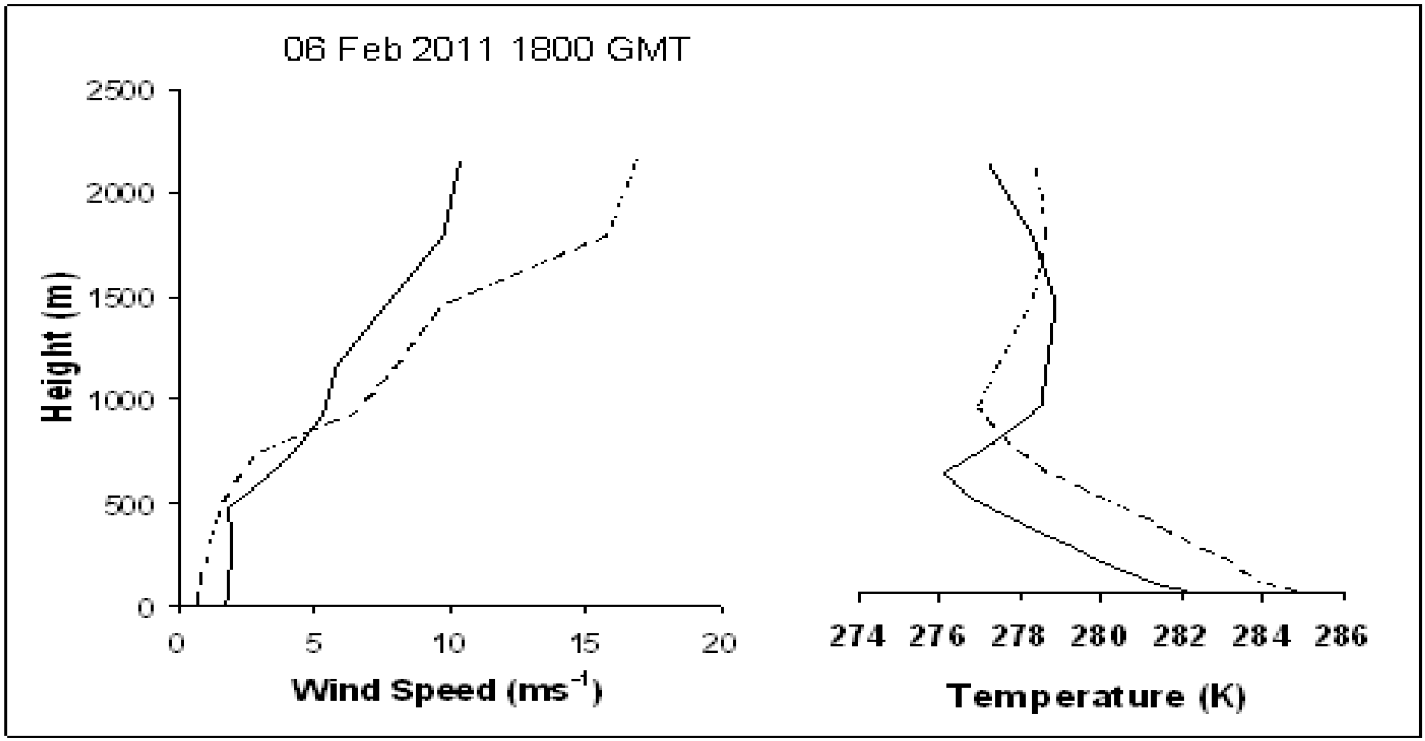
2.3. Data

A prescribed burn done on 6 February 2011 at Block 703C at Eglin Air Force Base, FL, USA, on a 660-ha (1,650 acre) tract (lat. 30.495N, long. 86.870W) was selected for several reasons. (1) The flat terrain of the lower coastal plain was not a factor in fire spread. (2) Ambient winds were weak through the depth of the mixing layer. Any significant winds were the outcome of fire-atmosphere coupling. (3) GPS coordinates of the aircraft taken during the mission pinpointed ignition locations. (4) Aerial ignition spreads fire widely over the landscape allowing for complex plume structures with multiple updraft cores. (5) A photo-image taken from a great distance from the plume validated model predictions of updraft core number. (6) Ceilometer measurements were taken for validation of Daysmoke predictions of plume rise. (7) The burn produced a strong, hot plume that penetrated well above the mixing layer thus providing a unique validation test for Daysmoke.

The tract had been burned in early March of 2009 and the 2-year fire return interval yielded relatively light fuel loadings—7 t/ha (3 ton/ac)—as determined from a stereo photo series for quantifying natural fuels [40]. A high-resolution Google Earth image capable of resolving individual trees was subjected to a color recognition scheme that yielded detailed spatial patterns of two fuel types—a mixture of grass and pine litter and grass only. Scattered herbaceous fuels were not considered in the fuels designation.

The helicopter-equipped GPS recorded the time and coordinates of each ignition during the 46-min mission (12:06–12:52 LST—local standard time). Ignition points were located with the assumption that the 6,000 ignition balls were dropped at the same rate during the flight. The balls were laid down in strips of roughly 100 m separation. The helicopter flew at an average speed of 7 ms⁻¹ along the straight-aways then slowed to turn around at the edges of the block. Greatest ball-drop densities therefore occurred at the edges where the helicopter slowed.

Table 1 summarizes the fuels data used to initialize Rabbit Rules. Fire residence times in the grass/pine needle mixture and the grass only fuel were set to, respectively, 0.5 min (30 s) and 0.1 min (6 s). Neither fuel was set for longer term smoldering although stochastic terms governing rabbit lifespan did increase some fire residence times to approximately 1.0 min. Fuel height proxies were, respectively, 0.65 m and 1.00 m. Vigor was set twice as large for the mixture to account for the 2-year accumulation of pine litter. The backspread factor (δ_Β ) was turned on meaning that coverages of both fuels were sufficiently dense that fire would spread upwind in light to moderate wind speeds. Other fuel parameters were held constant.

Daysmoke requires as input PM_2.5 released, total volume flux released during combustion and initial plume temperature. Total fuel consumption for the block 703C burn was determined using the single parameter regression equations for version 2.1 of CONSUME [41] as described in [9]. We calculated only 49,280 kg of PM_2.5 released during the active burn phase. Total PM_2.5 andvolume flux were proportioned in units per minute according to relative emissions production in Rabbit Rules. Initial plume temperature was set to ΔΤ₀ = 40 °C [38].

Weather data for both models were simulated by WRF [33] and MM5 [32] for 12:00–14:00 LST 6 February 2011. Figure 2 shows two vertical profiles of wind speed and temperature at 12:00 LST. The MM5 temperature profile (solid line) shows a neutral lapse rate through the mixing layer to 650 m capped by a deep stable layer. Wind speeds ranged from 1.5-2.5 ms⁻¹ through the mixing layer. The WRF temperature profile (dashed line) begins with a surface temperature 2.8 °C warmer and deepens the neutral lapse rate to 1,000 m. Wind speeds are typically 1.0 ms⁻¹ slower to 800 m then increase above the mixed layer to 6.5 ms⁻¹ faster at 2,000 m. In addition, a pibal sounding of winds, temperature, and relative humidity was taken at 09:00 LST, approximately 3-h before ignition.

Figure 2. Vertical profiles of wind speed and temperature for the first 2.2 km at Block 703C on 12:00 LST 6 February 2011. Solid lines are simulations by MM5 and dashed lines are simulations by WRF.

Figure 2. Vertical profiles of wind speed and temperature for the first 2.2 km at Block 703C on 12:00 LST 6 February 2011. Solid lines are simulations by MM5 and dashed lines are simulations by WRF.

On-site measurements relevant to this study were: Measurements of plume height taken with a Vaisala CL31 ceilometer, a LIDAR (Light Detection and Ranging) device [42]. The instrument was located 12.5 km northeast of the burn site. In addition, measurements of PM_2.5 were taken at three sites northeast of the burn. Further details of these and the ceilometer measurements are presented in the discussion of Daysmoke results.

3. Results

The results are divided into two sections. The first section summarizes variables generated by Rabbit Rules that are needed for initialization of Daysmoke. The second section summarizes the Daysmoke simulation for the case and validation of Daysmoke results.

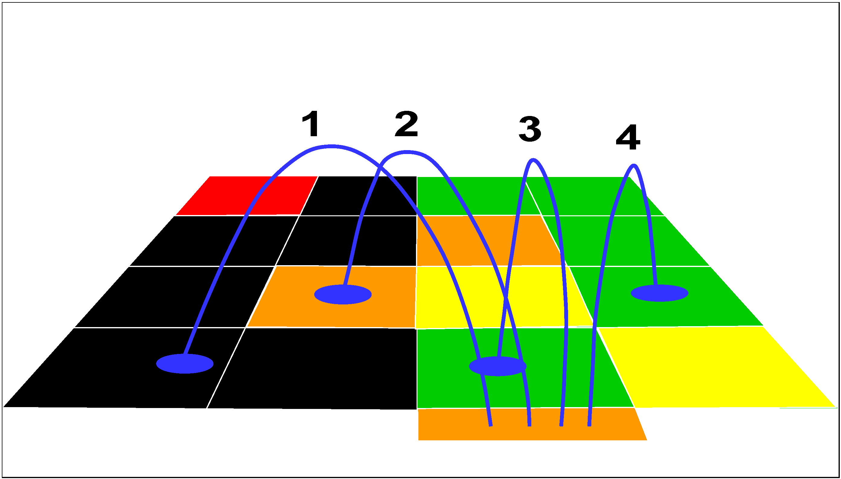
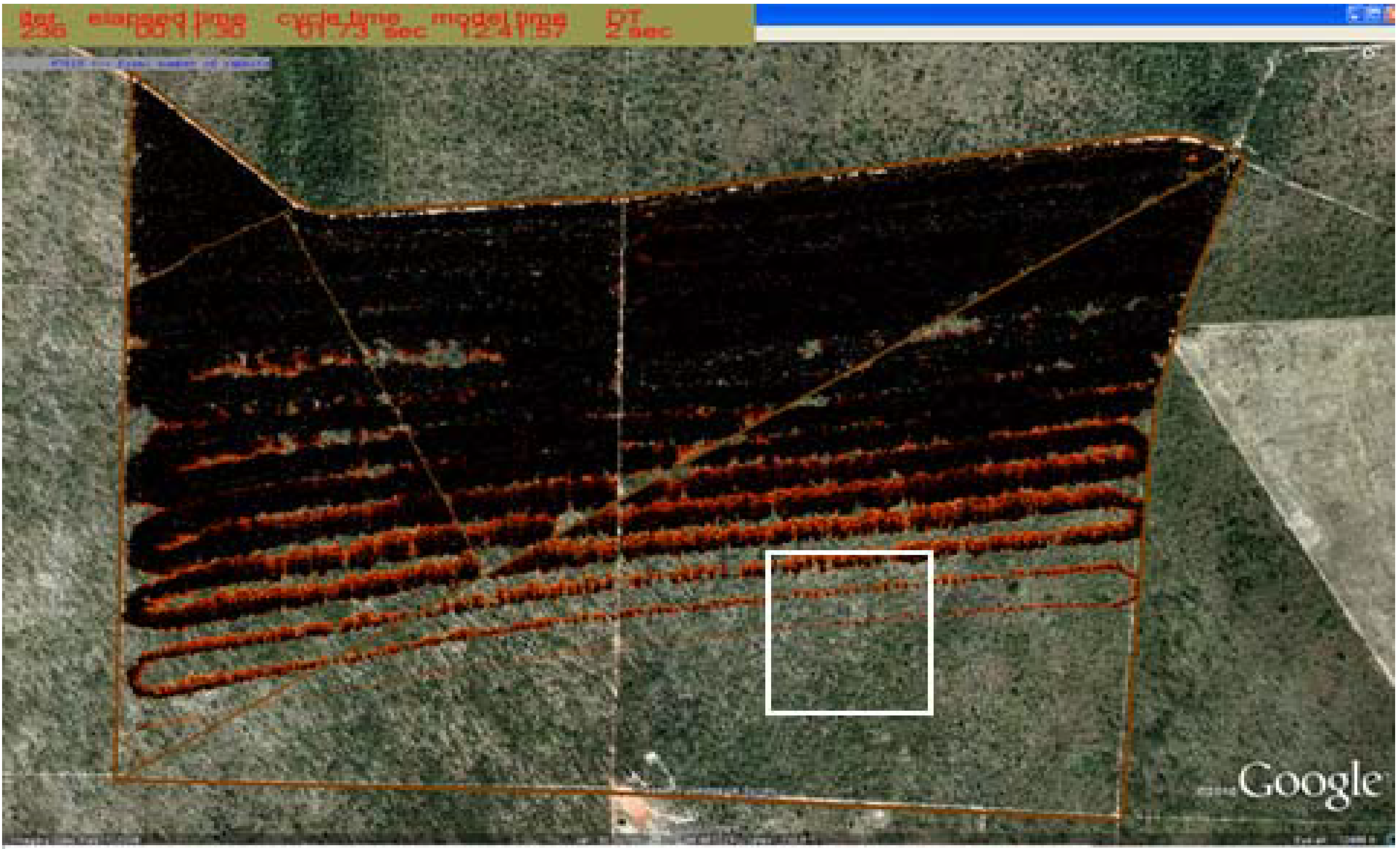
3.1. Core Number and Other Plume Initial Variables via Rabbit Rules

Given the short period of ignition (approximately 1 h), Rabbit Rules was run with the hourly average wind (12:00–13:00 LST) for 10 m (210 degrees at 1.3 ms⁻¹) and for 100 m (210 degrees at 1.5 ms⁻¹) in accord with the MM5 sounding (Figure 2).

Rabbit Rules was set to reproduce the helicopter pathway and the time rate of deposition of ignition balls beginning at 12:06 LST. Figure 3 shows the distribution of fire over the 660 ha tract at 12:41:57 LST. Fire expanded about the ignition points and merged with adjacent ignitions to form lines spaced at approximately 100 m. Average fire spread rate was 0.20 ms⁻¹.

Figure 3. Progress of helicopter ignition and burn-out for 12:41:57 6 February 2011.

Figure 3. Progress of helicopter ignition and burn-out for 12:41:57 6 February 2011.

The fire behavior in the presence of light ambient winds needs further explanation. Figure 4 shows an example of fire-atmosphere coupling within a sub-area of Block 703C (white square in Figure 3). The meteorological grid spacing is 60 m. Explanations of wind and fire behavior are given in reference to the center point (white dot). The first panel (12:32:43) shows the undisturbed prevailing 1.3 ms⁻¹ winds blowing from 210 degrees. By 12:40:02 (second panel) three lines of fire laid down by the helicopter are visible in the upper half of the figure. “Draw-in” of air toward the combustion zone accelerated the winds to 2.5 ms⁻¹ at the white dot. These winds increased to 4.0 ms⁻¹ at 12:44:55 toward a convergence axis (white dotted line) that locates the center-line of the smoke plume and beyond which winds were blowing from the north. The feed-back was a relatively intense faster-spreading head fire (12:46:58) which increased heat production and maintained the strong “draw-in”.

Figure 4. Fire-atmosphere coupling between winds and fire on the landscape within a sub-area of Figure 3.

Figure 4. Fire-atmosphere coupling between winds and fire on the landscape within a sub-area of Figure 3.

However, as the helicopter laid down new fire to the south and areas north of the center point burned out, the plume axis shifted south of the center point (12:49:50) in phase with the zone of maximum heat accumulation. Where the head fire had not burned to the adjacent fire line, the wind shifted to blow from the northwest at 5.0 ms⁻¹ and converted the head fire to a slow-moving backfire (12:51:00), creating islands of unburned fuel (12:52:03). As the plume axis moved farther away, the “draw-in” died down (12:53:44) allowing the backfire to consume the remaining fuel (12:58:39). Finally, winds returned to pre-burn ambient conditions (13:33:34). This sequence of helicopter lay-down of fire, followed by draw-in establishing a head fire, passage of the plume axis, local burn-out or conversion to backfire, to final burn-out was repeated over most of Block 703C.

The time-series of the north-south wind (v-component) at the center point in Figure 4 is shown in Figure 5. Draw-in ahead of the plume axis from 12:32–12:47 and draw-in behind the plume axis from 12:50–12:58 must be compensated by sinking of air from aloft. Slow-down and reversal of winds during the period from 12:47–12:50 must be compensated by updraft into the base of the plume. From the spatial distribution of the winds in Figure 4, it can be inferred that the maximum width for the plume base is not larger than twice the spacing of the meteorological grid or 120 m for this case.

Figure 5. Time series of the north-south wind at the center point shown in Figure 4.

Figure 5. Time series of the north-south wind at the center point shown in Figure 4.

Initial plume rise w₀ for conservation of flux into opposite sides of a box of height, h, and length, x, and up into a linear updraft of width y requires the vertical velocity within the plume above the convergence line in Figure 4 to obey

(10)

However, farther above ground, the updraft organizes into a string of n updraft cores of effective diameter, d. Thus,

(11)

where U₁ and U₂ represent flow through the opposite sides of the box.

For radial draw-in to a single updraft core (Figure 6), the flux of air through the sides of a cylinder of radius, r, and height, h, and draw-in speed, U₀, must equal the flux of air into the updraft core of effective diameter, d, and vertical velocity w₀. The equation for w₀ is,

(12)

For the convergence line (Equation (11)), substitution of the pertinent quantities (U₁ = 5.0 ms⁻¹ and U₂ = −5.0 ms⁻¹) yields w₀ = 2.12 h/n if x = 40Δx across the length of a fire line in Figure 2 and d = 2Δx (120 m). Thus w₀ depends on the choice for h and the number of updraft cores distributed along the length of the fire line. If h = 10 m, w₀ = 21.2/n. As regards radial draw-in (Equation 12), draw-in speed, U₀, and the radius, r, can be gotten from Figure 6, for example, U₀ = 6.3 ms⁻¹ on average at r = 3Δx. Furthermore, an estimate for the effective core diameter is d = 120 m. Thus w₀ = 0.63 h. If h = 10 m for the radial draw-in, w₀ = 6.3 ms⁻¹—about 25 percent of the estimate from the literature for effective plume diameter for a bent-over plume used by [9] and for the line convergence case, w₀ = 5.3 ms⁻¹ if n = 4. Deepening the draw-in depth to canopy height (if at 30 m) triples w₀. Reducing the effective core diameter also increases w₀. Therefore, reasonable estimates for initial updraft core vertical velocities range from 5.0–25.0 ms⁻¹.

Figure 6. Winds and divergence (1 unit = 0.012 s⁻¹) simulated by Rabbit Rules for a radial-inflow isolated updraft core at 12:22:52. Wind speed convention is the same as that for Figure 4.

Figure 6. Winds and divergence (1 unit = 0.012 s⁻¹) simulated by Rabbit Rules for a radial-inflow isolated updraft core at 12:22:52. Wind speed convention is the same as that for Figure 4.

Figure 7. Pressure anomalies (white lines) generated by Rabbit Rules at 12:40:41. The yellow ellipses highlight centers that might correspond to updraft cores.

Figure 7. Pressure anomalies (white lines) generated by Rabbit Rules at 12:40:41. The yellow ellipses highlight centers that might correspond to updraft cores.

Figure 8. Photo-image of the Block 703C plume taken from a bridge 42 km east-southeast from the burn.

Figure 8. Photo-image of the Block 703C plume taken from a bridge 42 km east-southeast from the burn.

Needed to complete calculations for initial plume dynamics is a mechanism for estimating updraft core number. From Equation (5), areas of heat accumulation into an incipient plume are represented in Rabbit Rules by low pressure anomalies. During the simulation of fire spread, pressure anomalies ranged as low as −1.4 mb and the number ranged from one to six but typically was four. At 12:40:41 (Figure 7), largest pressure anomalies of −1.0 mb are located along the zone of maximum fire near the boundaries of Block 703C. A minor center of −0.4 mb is located behind. The yellow ellipses highlight locations of pressure anomaly centers that could direct the winds into updraft cores. The large ellipse encloses three centers joined by an axis of low pressure. It is inferred that these could merge into a single updraft core a short distance above the ground.

Figure 9. Relative emissions as a function of total emissions for the Block 703C burn as simulated by Rabbit Rules.

Figure 9. Relative emissions as a function of total emissions for the Block 703C burn as simulated by Rabbit Rules.

The multiple-core updraft structure of the Block 703C burn is shown by a photo-image taken from a location 42 km east-southeast from the burn (Figure 8). There were two prominent updraft cores on the far left and far right of the burn (long arrows). In the center, there appear either two closely spaced updraft cores or two updraft cores that merge into one updraft core partway in ascent (two small arrows). The time of the photo-image was not taken. However, the extent of spread of the plume top would infer that the image was taken midway or later during the burn.

Finally, Rabbit Rules provides time-series of relative emissions expressed as a percentage of total emissions per minute. Figure 9 shows that relative emissions peaked twice, first at minute 738 (12:18 LST) to 2.73 percent of total emissions at minute, then to 4.26 percent at minute 760 (12:42 LST).

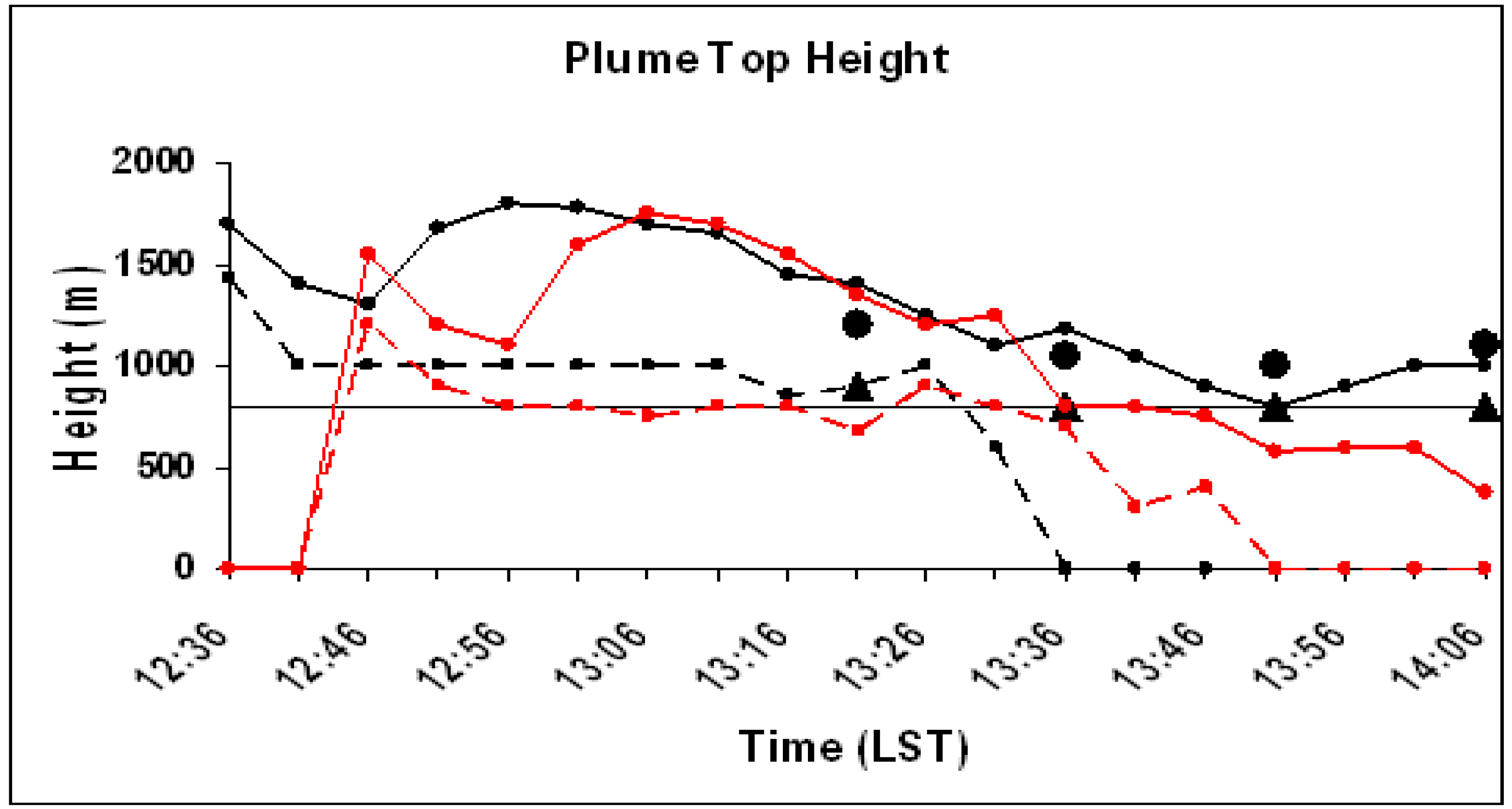
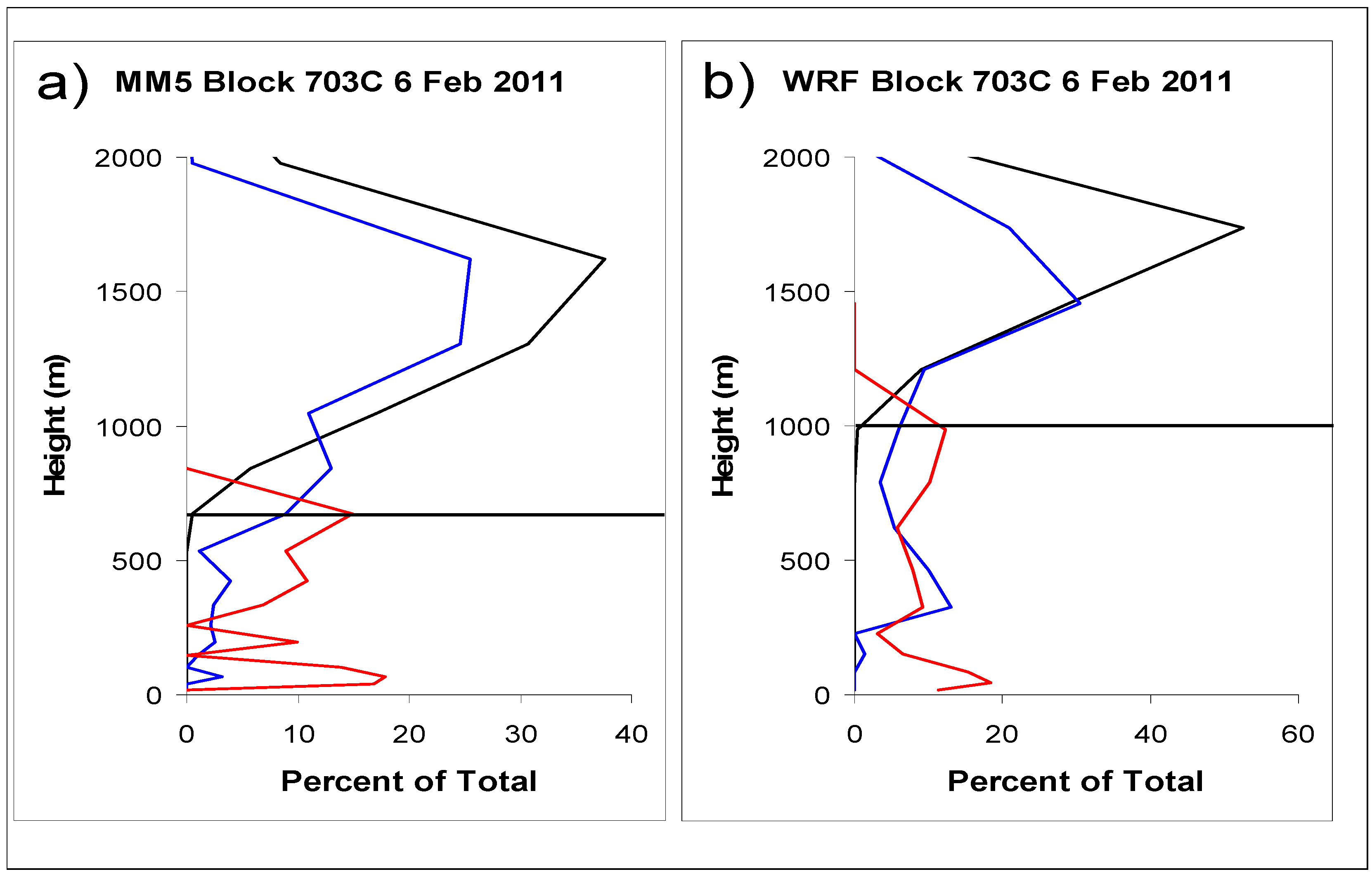
3.2. Plume Rise and Particulate Concentration via Daysmoke

In past studies, w₀ and ΔΤ₀ were set to, respectively, 25 ms⁻¹ and 40 K for grass fires [38]. However, these inputs may not be valid for fire in southern United States pine forests. Depending on assumptions, the initial vertical velocities calculated from Rabbit Rules ranged from 5–25 ms⁻¹. Further reductions on transfer of momentum from the plume to the trees through canopy drag should be expected. Furthermore, transfer of heat from the plume passing through the canopy would be expected to reduce the initial temperature anomaly. Thus the initial vertical velocities for the four updraft cores were set to range from 8–12 ms⁻¹ stochastically (shaded area in Figure 10a) and the initial temperature anomaly was set to 30 K. These numbers are approximate and more accurate estimates await future research.

Figure 10. 1-min time-series from Rabbit Rules for (a) Initial vertical velocity and (b) Initial effective plume diameter for the range of updraft cores calculated for the 6 February 2011 burn.

Figure 10. 1-min time-series from Rabbit Rules for (a) Initial vertical velocity and (b) Initial effective plume diameter for the range of updraft cores calculated for the 6 February 2011 burn.

Total mass flux (in units of mass flux per minute) and total PM_2.5 (49,280 kg)was partitioned from 12:00 LST (minute 720) to 13:20 LST (minute 800) according to the relative emissions production simulated in Rabbit Rules (Figure 9). Thus updraft cores were recalculated for every minute. The volume fluxes of the individual updraft cores were defined subject to the constraints put forth in the derivation of Equation (9). The range of initial plume diameters D_0k (shaded area in Figure 10b) were calculated by replacing f₀ with f_k in Equation (8).

Figure 11 shows 5-min time-series of MM5 and WRF-simulated maximum plume top height and plume depth calculated at a reference distance of 12.5 km (7.8 mi) along the plume axis (red asterisk for MM5 in Figure 12) equal to the distance of the ceilometer (yellow square) from the burn. Note that Daysmoke plume heights were obtained from a “projected cross section”—all smoke points were projected onto a vertical plane (arrow) extending from the burn site along the plume axis. Therefore the maximum heights and the minimum heights contained in the cross-sections do not exactly represent plume structures observed at the ceilometer located approximately 3.7 km from the plume centerline.

Figure 11. Plume top heights and bases of Daysmoke simulations based on WRF (black lines—solid and dashed) and MM5 (red lines—solid and dashed). The plume data were calculated from Daysmoke at 12.5 km (7.8 mile) downwind from the burn. Plume tops and bases observed by ceilometer are given, respectively, by the large circles and triangles.

Figure 11. Plume top heights and bases of Daysmoke simulations based on WRF (black lines—solid and dashed) and MM5 (red lines—solid and dashed). The plume data were calculated from Daysmoke at 12.5 km (7.8 mile) downwind from the burn. Plume tops and bases observed by ceilometer are given, respectively, by the large circles and triangles.

After ascent into the free atmosphere above the mixed layer, the plume was subject to stronger transport winds in the WRF sounding than in the MM5 sounding (Figure 2). Regarding the WRF-based simulation, the maximum plume top of 1,800 m traveled at 6.9 ms⁻¹ to arrive at the reference distance at 12:56 (solid black line in Figure 11). That was approximately 10-min before the arrival of the 1,750 m plume top in the simulation using the MM5 sounding (solid red line in Figure 11) which was traveling at 5.2 ms⁻¹. The plume top height minimum at 16:46 (WRF) and 16:56 (MM5) corresponds to the minimum in relative emissions at minute 18 in Figure 9 and the minimum in updraft core diameter at 18 min after ignition in Figure 10b.

Ceilometer observations of plume top height (large circles) began at 13:21 and declined slowly from 1,200 m to 1,000 m at 13:51 then rose again to 1,100 m at 13:56. Both Daysmoke simulations came into agreement after 13:06 having declined from the maxima to 1,400 m (1,350 m) by 13:21 after which the time-series for the WRF-based simulation (black line) continued in relatively good agreement with the observed plume top heights through 14:06. After 13:36, the time-series for the MM5-based simulated plume tops (red line) fell below the observed plume base (solid triangles).

Figure 12. Ground-level PM_2.5 average concentrations above background simulated for a 2-hour period beginning at ignition for the MM5 meteorological sounding. The small squares represent 1 mi (1.6 km) and the light green square represents 10 mi (16 km). The axis of the plume is given by the white arrow. Also shown are locations of the ceilometer (yellow square) and three PM_2.5 sampling units (red triangles).

Figure 12. Ground-level PM_2.5 average concentrations above background simulated for a 2-hour period beginning at ignition for the MM5 meteorological sounding. The small squares represent 1 mi (1.6 km) and the light green square represents 10 mi (16 km). The axis of the plume is given by the white arrow. Also shown are locations of the ceilometer (yellow square) and three PM_2.5 sampling units (red triangles).

Figure 13. A projected vertical cross-section showing the Daysmoke simulation of the Block 703C burn (WRF sounding) at 12:56 LST. The mixing height is given by the horizontal white line. The “reference distance” is shown by the white arrow.

Figure 13. A projected vertical cross-section showing the Daysmoke simulation of the Block 703C burn (WRF sounding) at 12:56 LST. The mixing height is given by the horizontal white line. The “reference distance” is shown by the white arrow.

The ceilometer also observed a well-defined plume thickness of approximately 300 m thus giving plume base as shown by the solid triangles. Both MM5 and WRF-based simulations gave plume bases (dashed lines) defined by the mixing height. Thus the WRF-based plume thickness was 800 m at maximum plume height and declined to 400 m by 13:21. However a projected vertical cross-section of the simulation at 12:56 (Figure 13) showed most “smoke” concentrated within an approximate 300 m layer below the plume top.

Average above background ground-level concentrations of PM_2.5 for the Daysmoke simulation with the MM5 sounding for the period 12:00–14:00 LST are shown in Figure 12. The scattering of white circles along the general plume axis represents above-background concentrations due to smoke of 1–2 μg m⁻³. Note that simulations were for flaming stage only. Measurements of PM_2.5 taken at the three sites identified by the red triangles are shown in Figure 14. No smoke was observed at Site 3 (green line) and the absence of smoke at Site 2 (blue line) confirms ceilometer observations of the plume base remaining above 800 m. Smoke was observed at Site 1 after 13:36 at the same time as smoke arrived at the reference distance (red asterisk). Daysmoke did not simulate smoke at Site 1. Therefore the near-simultaneous arrival of smoke at two disparate locations can be explained if smoke was from different sources. Projected vertical cross-sections of the Daysmoke simulations are suggestive that smoke arriving at the reference distance was transported down by convective circulations from the overhead plume passing at higher wind speeds near the top of the mixing layer. Smoke arriving at Site 1 within surface winds blowing at 1.5 ms⁻¹ would have departed the closest perimeter of Block 703C 28 min earlier or at approximately 13:08. Aerial ignition had ceased by 12:52. Thus, allowing time for burnout, the source of smoke at Site 1 was likely from smoldering combustion. Figure 14 shows that concentrations increased reaching a maximum at 13:55 LST and remaining at elevated levels thereafter.

Figure 14. Measurements of PM_2.5 taken at the three sites in Figure 12: Site 1 (red), Site 2 (blue) and Site 3 (green).

Figure 14. Measurements of PM_2.5 taken at the three sites in Figure 12: Site 1 (red), Site 2 (blue) and Site 3 (green).

If little flaming phase smoke was recorded and simulated at the ground, where did the smoke go? Daysmoke also functions as a smoke injector for the regional scale air quality model CMAQ [43]. The amount of smoke injected into a model layer per hour is the smoke passing through a cylinder of radius 11 km (7 mile) at height equal to the layer of interest—the cylinder radius chosen to allow Daysmoke to fully develop the plume. The vertical distribution of smoke shown in Figure 15a (based on the MM5 sounding) has been normalized by layer thickness and is expressed as a percentage of the total smoke passing through the walls of the cylinder for that hour. The mixing height is given by the thin black line at 650 m. For the period 12:00–13:00 LST (black line) 100 percent of the smoke passing through the wall was above the mixing height where ambient winds were strong enough to carry smoke to the wall. Roughly 84 percent of the smoke passing through the cylinder during the hour ending at 14:00 LST was found above the mixing layer (blue line). At 15:00 LST (red line) most of the smoke was confined to the mixing layer but this accounted for only 3.5 percent of the total for the burn. Overall, 93 percent of the smoke was confined above the mixing layer. Note that these calculations were done only for particulate matter released during the flaming phase.

Figure 15. For the Daysmoke simulation done with the (a) MM5 and (b) WRF soundings: Vertical distribution of smoke within normalized by layer thicknesses and expressed as a percentage of the total smoke passing through a wall of an 11 km radius cylinder for 13:00 LST (black line), 14:00 LST (blue line) and 15:00 LST (red line).

Figure 15. For the Daysmoke simulation done with the (a) MM5 and (b) WRF soundings: Vertical distribution of smoke within normalized by layer thicknesses and expressed as a percentage of the total smoke passing through a wall of an 11 km radius cylinder for 13:00 LST (black line), 14:00 LST (blue line) and 15:00 LST (red line).

Similar results were found for the simulation done with the WRF sounding (Figure 15b). Note the mixing height at 1,000 m. As could be expected from the time-series of plume top heights (Figure 11), particulate concentrations were found higher at 13:00 LST than those for the MM5 sounding. By 15:00 LST (red line), all smoke was confined below the mixing height. For the total active burn phase, 89 percent of the smoke was confined above the mixing height.

4. Discussion

Smoke plumes from wildland fire (prescribed and wildfire), are complex in structure with plumes typically defined by a number of updraft cores. The multiple-core structure has implications for modeling plume rise as the total mass/volume flux from combustion distributed over many updraft cores, relative to a single updraft core, must be conserved. Multiple-core updraft plumes have larger total surface area to volume ratios than does a single core, are more exposed to entrainment, and grow to lower heights. Previous research with Daysmoke [9] has shown that specification of updraft core number is the single-most important model parameter for predicting plume rise from prescribed burns.

Simulations of weak plumes by Daysmoke [9] were done through subjectively “estimating” updraft core number by taking into consideration factors such as size and shape of the burn area, fuel type, moisture, loadings and heterogeneity, amount and distribution of fire on the landscape, distribution of canopy gaps, transport wind speed, and mixing layer depth. That study brought into question the appropriateness of equating initial plume updraft vertical velocity for prescribed burns in southern United States pinelands with initial plume updraft vertical velocity simulated by a full-physics fire model for grass fires. In addition, comparisons between model-simulated PM_2.5 and high-frequency measurements from real-time samplers revealed a need for an improved emissions production model.

In this study we evaluated Daysmoke for a strong plume from a helicopter aerial ignition prescribed burn conducted on 6 February 2011 at Eglin AFB, USA. Because the track of ignition times and locations was fixed by an onboard GPS unit, Daysmoke could be coupled with the experimental CA fire model, Rabbit Rules, by using the latter to deduce initial conditions required by the former. The CA fire model showed the importance of fire-atmosphere coupling in fire spread rate and fire intensity. Fire-atmosphere coupling increased winds locally from less than 2 ms⁻¹ to 10 ms⁻¹. Lines of more intense fire coupled with winds to create low pressure anomaly centers with each center assumed to represent the base of an updraft core.

The numbers of pressure anomaly centers simulated in Rabbit Rules were counted for each minute during the burn. Updraft cores ascending above small, weak centers were assumed to have been absorbed into nearby stronger updraft cores. Furthermore, adjacent strong pressure anomaly centers were assumed to have merged into single updraft cores a short distance aloft as implied by the centers within the large ellipse in Figure 7. This assumption is supported by how the main plume (rightmost updraft core in Figure 8) organized from smoke originating from sources spread out near the ground and the possibility that the two central cores (small arrows) merged into a single core. The final number of updraft cores ranged from one to six with the most frequent number being four. Three/four updraft cores were visible in the photo-image (Figure 8).

In addition, Rabbit Rules supplied initial updraft vertical velocities and relative emissions in percent of total emissions per minute, as initial conditions for Daysmoke. Depending on assumptions made, the initial updraft vertical velocities were found in the range 5–25 ms⁻¹.

Daysmoke was set with four updraft cores throughout the burn. Initial updraft vertical velocities for the four updraft cores were set to range between 8–12 ms⁻¹ stochastically. These and the method for calculating updraft core diameter given in Equation (9) produced the ranges of initial vertical velocity and updraft core diameter shown in Figure 10. The initial temperature anomaly was set to 30 K. Simulations with atmospheric soundings from WRF and MM5 produced plume tops that overshot the mixing height from 800–1,100 m. Plume tops above the mixing height were confirmed by ceilometer measurements. Particulate matter ejected into the free atmosphere above the mixing layer during the active flaming stage ranged from 89–93 percent.

The impact of the forest canopy on the simulations needs further explanation. In [9] we argued that passage of the plume through forest canopies must involve significant momentum and heat transfer from the plume to the crown. The impact of the forest canopy on Daysmoke may be to convert an incipient small diameter, relatively warm, fast-rising bent-over plume into a large diameter, relatively cool, slow-rising highly-tilted plume capable of ascending higher than its bent-over counterpart. However, this conclusion was based on the assumption of conservation of mass/volume flux. The impact of a closed forest canopy on Rabbit Rules may be to reduce the mass/volume flux. Increased fuels deposition from a dense over-story of a closed canopy relative to an open canopy would be expected to increase fuel loadings and thus increase fire intensity. However, sheltering of the fuel bed from wind and sun may retain higher fuel moisture under closed canopy thus decreasing fire intensity. Furthermore, reduced ambient wind speeds under a closed canopy should contribute to decreased fire intensity through slowing fire spread rates. In extreme conditions, fire confined under a closed canopy may suffer from oxygen deficiency thus further reducing fire intensity.

Canopy characteristics for the block 703C burn mostly ranged from open to partially closed. For Daysmoke, initial updraft vertical velocities were reduced from 25 ms⁻¹ to from 8–12 ms⁻¹ and initial temperature anomaly reduced from 40 K to 30 K in comparison with [9] to partially estimate canopy effects. No adjustments were made in Rabbit Rules beyond the fuel designations shown in Table 1. Fire behavior under a closed canopy relative to fire behavior under an open canopy is a subject for further research the outcome of which could be an additional fuel designation vector in Table 1 or a canopy rule for the CA fire model.

5. Conclusions

The Daysmoke plume rise model is planned for injecting smoke from prescribed burns into regional scale air quality models. The lack of quantitative initialization data, in particular, the number of updraft cores that define the plume has limited the accuracy of Daysmoke simulations. In this paper, we successfully coupled Daysmoke with the experimental CA fire model, Rabbit Rules, by using the latter to calculate initial conditions for the former. The coupling can be tighter pending an algorithm that calculates updraft core numbers and diameters from mergers of pressure anomaly centers. Then updraft core data coupled with relative emissions data simulated by Rabbit Rules will enable calculation of emissions for each core.

Although Rabbit Rules offers a solution for the updraft core problem posed in Daysmoke, limitations of both models as currently configured should be noted. First, both Daysmoke and Rabbit Rules have been designed for and validated against prescribed burns—Daysmoke for weak plumes [9] and a strong plume (this study) and Rabbit Rules for a grass fire [24,39] and for aerial ignition in pinelands (this study). Most prescribed burning is done within the gently rolling Piedmont and flat coastal plains of the southern United States—areas for which the models have been validated. Neither model has yet been applied for burns over mountainous terrain. Second, no studies to date have been done for wildfires spread over large landscapes and which can generate extreme conditions of plume rise and fire-atmosphere coupling. Validation under these conditions is a subject for future study.

Furthermore, detailed ignition data are not available from most prescribed burns. Therefore the ranges of initial conditions for Daysmoke will be determined from a slowly growing number of experimental burns. Then, for other burns, Daysmoke will be initialized from these data using methods yet to be determined.

Finally, ongoing simulations with Daysmoke continue to show that when and where heat and particulate matter are released into the atmosphere are complicated by evolving atmospheric conditions during the burn. From earlier studies of weak plumes, nearly 100 percent of smoke was confined to the mixing layer. This is not always the case for strong plumes (as in this study) which are typically associated with larger-area burns and therefore larger amounts of particulate matter released. For air quality prediction models, both levels and timing of smoke injection may be critical for accurate prediction of local and regional distributions of particulate matter.

References

- Wade, D.D.; Brock, B.L.; Brose, P.H.; Grace, J.B.; Hoch, G.A.; Patterson, W.A., III. Fire in Eastern Ecosystems. In Wildland Fire in Ecosystems: Effects of Fire on Flora; Brown, J.K., Smith, J.K., Eds.; Department of Agriculture: Forest Service, Rocky Mountain Research Station: Ogden, UT, USA, 2000; Volume 2, pp. 53–96. Chapter 4. [Google Scholar]
- Achtemeier, G.L. Effects of moisture released during forest burning on fog formation and implications for visibility. J. Appl. Meteorol. Climatol. 2008, 47, 1287–1296. [Google Scholar] [CrossRef]
- Achtemeier, G.L. On the formation and persistence of superfog in woodland smoke. Meteorol. Appl. 2009, 16, 215–225. [Google Scholar] [CrossRef]
- Naeher, L.P.; Achtemeier, G.L.; Glitzenstein, J.S.; MacIntosh, D.; Streng, D.R. Real-time and time-integrated PM2.5 and CO from prescribed burns in chipped and non-chipped plots—Firefighter and community exposure and health implications. J. Expo. Sci. Environ. Epidemiol. 2006. Available online: http://www.nature.com/doifinder/10.1038/sj.jea.7500497 (accessed on 10 July 2012).
- Lee, S.; Russell, A.G.; Baumann, K. Source apportionment of fine particulate matter in the southeastern United States. J. Air Waste Manag. Assoc. 2007, 57, 1123–1135. [Google Scholar] [CrossRef]
- Hu, Y.M.; Odman, T.; Chang, M.E.; Jackson, W.; Lee, S.; Edgerton, E.S.; Baumann, K. Simulation of air quality impacts from prescribed fires on an urban area. Environ. Sci. Technol. 2008, 42, 3676–3682. [Google Scholar]
- Byun, D.W.; Ching, J. Science Algorithms of the EPA Model-3 Community Multiscale Air Quality (CMAQ) Modeling System; EPA/600/R-99/030; National Exposure Research Laboratory: Research Triangle Park, NC, USA, 1999. [Google Scholar]
- Byun, D.W.; Schere, K.L. Review of the governing equations, computational algorithms, and other components of the Models-3 Community Multiscale Air Quality (CMAQ) modeling system. Appl. Mech. Rev. 2006, 59, 51–77. [Google Scholar] [CrossRef]
- Achtemeier, G.L.; Goodrick, S.A.; Liu, Y.; Garcia-Menendez, F.; Hu, Y.; Odman, M.T. Modeling plume-rise and smoke dispersion from southern United States prescribed burns. Atmosphere 2011, 2, 358–388. [Google Scholar]
- Oberhuber, J.M.; Herzog, M.; Graf, H.-F.; Schwanke, K. Volcanic plume simulation on large scales. J. Volcanol. Geotherm. Res. 1998, 87, 29–53. [Google Scholar]
- Herzog, M.; Graf, H.-F.; Textor, C.; Oberhuber, J.M. The effect of phase changes of water on the development of volcanic plumes. J. Volcanol. Geotherm. Res. 1998, 87, 55–74. [Google Scholar] [CrossRef]
- Freitas, S.R.; Longo, K.M.; Chatfield, R.; Latham, D.; Silva Dias, M.A.F.; Andreae, M.O.; Prins, E.; Santos, J.C.; Gielow, R.; Carvalho, J.A., Jr. Including the sub-grid scale plume rise of vegetation fires in low resolution atmospheric transport models. Atmos. Chem. Phys. 2007, 7, 3385–3398. [Google Scholar]
- Freitas, S.R.; Longo, K.; Trentmann, J.; Latham, D. Including the Environmental Wind Effects on Smoke Plume Rise of Vegetation Fires in 1D Cloud Models. In Proceedings of the Eighth Symposium on Fire and Forest Meteorology, Kalispell, MT, USA, 13–15 October 2009.
- Liu, Y.Q.; Achtemeier, G.L.; Goodrick, S.; Jackson, W.A. Important parameters for smoke plume rise simulation with Daysmoke. Atmos. Pollut. Res. 2010, 1, 250–259. [Google Scholar]
- Clarke, K.C.; Brass, J.A.; Riggan, P.J. A cellular automaton model of wildfire propagation and extinction. Photogramm. Eng. Remote Sens. 1994, 60, 1355–1367. [Google Scholar]
- Clarke, K.C.; Olsen, G. Refining a Cellular Automaton Model for Wildfire Propagation and Extinction. In GIS and Environmental Modeling: Progress and Research Issues; Goodchild, M.F., Louis, T., Steyaert, L.T., Bradley, O., Parks, B.O., Johnston, C., Eds.; John Wiley and Sons Publishers: Hoboken, NJ, USA, 1996. [Google Scholar]
- Karafyllidis, I.; Thanailakis, A. A model for predicting forest fire spreading using cellular automata. Ecol. Model. 1997, 99, 87–97. [Google Scholar] [CrossRef]
- Metzler, R.; Klafter, J. The random walk’s guide to anomalous diffusion: A fractional dynamics approach. Phys. Rep. 2000, 339, 1–77. [Google Scholar]
- Berjak, S.G.; Hearne, J.W. An improved cellular automaton model for simulating fire in a spatially heterogeneous Savanna system. Ecol. Model. 2002, 148, 133–151. [Google Scholar]
- Sullivan, A.L.; Knight, I.K. A Hybrid Cellular Automata/Semi-Physical Model of Fire Growth. In. In Proceedings of the 7th Asia-Pacific Conference on Complex Systems, Cairns, Australia, 6–10 December 2004; pp. 64–73.
- Encinas, A.H.; Encinas, L.H.; White, S.H.; Martin del Rey, A.; Rodriguez Sanchez, G. Simulation of forest fire fronts using cellular automata. Adv. Eng. Softw. 2007, 38, 372–378. [Google Scholar]
- Yassemi, S.; Dragicevic, S.; Schmidt, M. Design and implementation of an integrated GIS-based cellular automata model to characterize forest fire behavior. Ecol. Model. 2008, 210, 71–84. [Google Scholar]
- Adou, J.K.; Billaud, Y.; Brou, D.; Clerc, J.-P.; Consalvi, J.-L.; Fuentes, A.; Kaiss, A.; Nmira, F.; Porterie, B.; Zekri, L.; Zekri, N. Simulating wildfire patterns using a small-world network model. Ecol. Model. 2010. [Google Scholar]
- Achtemeier, G.L. Field validation of a free-agent cellular automata model of fire spread. Int. J. Wildland Fire 2012. [Google Scholar]
- Clark, T.L.; Jenkins, M.A.; Coen, J.; Packham, D. A coupled atmospheric-fire model: Convective Froude number and dynamic fingering. Int. J. Wildland Fire 1996, 6, 177–190. [Google Scholar]
- Linn, R.R.; Cunningham, P. Numerical simulations of grass fires using a coupled atmosphere-fire model: Basic fire behavior and dependence on wind speed. J. Geophys. Res. 2005, 110. [Google Scholar]
- Flakes, G.W. The Computational Beauty of Nature: Computer Explorations of Fractals, Chaos, Complex Systems, and Adaptation; MIT Press: Cambridge, MA, USA, 2000. [Google Scholar]
- Andrews, P.L.; Bevins, C.D.; Seli, R.C. BehavePlus Fire Modeling System, Version 3.0: User’s Guide; Gen. Tech. Rep. RMRS-GTR-106WWW Revised; U.S. Department of Agriculture: Forest Service, Rocky Mountain Research Station: Ogden, UT, USA, 2005. [Google Scholar]
- Hargrove, W.W.; Gardner, R.H.; Turner, M.G.; Romme, W.H.; Despain, D.G. Simulating fire patterns in heterogeneous landscapes. Ecol. Model. 2000, 135, 243–263. [Google Scholar] [CrossRef]
- Andrews, P.L. BehavePlus Fire Modeling System Version 4.0: Variables; Gen. Tech. Rep. RMRS-GTR-213WWW; U.S. Department of Agriculture: Forest Service, Rocky Mountain Research Station: Washington, DC, USA, 2008. [Google Scholar]
- Achtemeier, G.L. Planned burn-Piedmont. A local operational numerical meteorological model for tracking smoke on the ground at night: Model development and sensitivity tests. Int. J. Wildland Fire 2005, 14, 85–98. [Google Scholar] [CrossRef]
- Grell, G.A.; Dudhia, J.; Stauffer, D.R. A Description of the Fifth-generation Penn State/NCAR Mesoscale Model (MM5); NCAR Tech. Note NCAR/TN-3921STR; NCAR: Boulder, CO, USA, 1994. [Google Scholar]
- Skamarock, W.C.; Klemp, J.B.; Dudhia, J.; Gill, D.O.; Barker, D.M.; Wang, W.; Powers, J.G. A Description of the Advanced Research WRF Version 2; NCAR Technical Note: NCAR/TN-468+STR; NCAR: Boulder, CO, USA, 2005. [Google Scholar]
- Achtemeier, G.L. Predicting dispersion and deposition of ash from burning cane. Sugar Cane 1998, 1, 17–22. [Google Scholar]
- Achtemeier, G.L.; Adkins, C.W. Ash and smoke plumes produced from burning sugar cane. Sugar Cane 1997, 2, 16–21. [Google Scholar]
- Byram, G.M. Combustion of Forest Fuels. In Forest Fire Control and Use; Davis, K.P., Ed.; McGraw Hill: New York, NY, USA, 1959; pp. 155–182. [Google Scholar]
- Mercer, G.N.; Weber, R.O. Fire Plumes. In Forest Fires: Behavioral and Ecological Effects; Johnson, E.A., Miyanishi, K., Eds.; Academic Press: New York, NY, USA, 2001. [Google Scholar]
- Jenkins, M.A.; Clark, T.; Coen, J. Coupling Atmospheric and Fire Models. In Forest Fires: Behavior and Ecological Effects; Johnson, E.A., Miyanishi, K., Eds.; Academic Press: San Diego, CA, USA, 2001; pp. 258–301. [Google Scholar]
- Clements, C.B.; Zhong, S.; Goodrick, S.; Li, J.; Potter, B.E.; Bian, X.; Heilman, W.E.; Charney, J.J.; Perna, R.; Jang, M.; et al. Observing the dynamics of wildland grass fires: FireFlux-A field validation experiment. Bull. Am. Meteor. Soc. 2007, 88, 1369–1382. [Google Scholar] [CrossRef]
- Ottmar, R.D.; Vihnanek, R.E.; Mathey, J.W. Stereo Photo Series for Quantifying Natural Fuels. Vol. VIa: Sand Hill, Sand Pine Scrub, and Hardwoods with White Pine Types in the Southeast United States with Supplemental Sites for Volume VI; PMS 838 NFES 1119; US Department of the Interior: Washington, DC, USA, 2003; p. 22. [Google Scholar]
- Ottmar, R.D.; Anderson, G.K.; DeHerrera, P.J.; Reinhardt, T.E. Consume Version 2.1 User’s Guide; Department of Agriculture, Forest Service, Pacific Northwest Research Station: Portland, OR, USA, 1999. Available online: http://www.fs.fed.us/pnw/fera/products/consume/CONSUME21_USER_GUIDE.DOC (accessed on 10 July 2012).
- Liu, Y.Q.; Goodrick, S.A.; Achtemeier, G.L.; Forbus, K.; Combs, D. Smoke plume height measurements of prescribed burns in the southeastern United States. Int. J. Wildland Fire 2011. [Google Scholar]
- Liu, Y.Q.; Goodrick, S.; Achtemeier, G.L.; Jackson, W.A.; Qu, J.J.; Wang, W. Smoke incursions into urban areas: Simulation of a Georgia prescribed burn. Int. J. Wildland Fire 2009, 18, 336–348. [Google Scholar]
© 2012 by the authors; licensee MDPI, Basel, Switzerland. This article is an open-access article distributed under the terms and conditions of the Creative Commons Attribution license (http://creativecommons.org/licenses/by/3.0/).
Share and Cite
Achtemeier, G.L.; Goodrick, S.A.; Liu, Y. Modeling Multiple-Core Updraft Plume Rise for an Aerial Ignition Prescribed Burn by Coupling Daysmoke with a Cellular Automata Fire Model. Atmosphere 2012, 3, 352-376. https://doi.org/10.3390/atmos3030352
Achtemeier GL, Goodrick SA, Liu Y. Modeling Multiple-Core Updraft Plume Rise for an Aerial Ignition Prescribed Burn by Coupling Daysmoke with a Cellular Automata Fire Model. Atmosphere. 2012; 3(3):352-376. https://doi.org/10.3390/atmos3030352
Chicago/Turabian StyleAchtemeier, Gary L., Scott A. Goodrick, and Yongqiang Liu. 2012. "Modeling Multiple-Core Updraft Plume Rise for an Aerial Ignition Prescribed Burn by Coupling Daysmoke with a Cellular Automata Fire Model" Atmosphere 3, no. 3: 352-376. https://doi.org/10.3390/atmos3030352