1. Introduction
Aerosols have significant impacts on climate [
1] and air quality [
2]. Measurements of aerosol abundances and microphysical properties are necessary for monitoring their distribution and for providing insight into the physical processes governing their environmental impacts. Theoretical sensitivity studies, e.g., [
3,
4] and observations from aircraft and spacecraft suggest that passive remote sensing of aerosol microphysics (using reflected sunlight as the illumination source) benefits from multispectral and multiangular observations, and is enhanced through incorporation of polarization, e.g., [
5,
6,
7,
8,
9,
10]. Radiative transfer calculations [
3] imply that in order to meet the stringent requirements of aerosol climate impact assessments [
11], inclusion of polarimetry with uncertainty in degree of linear polarization (DOLP) less than ±0.005 improves significantly upon the information content of multiangular spectral intensity measurements.
To advance our understanding of the climate and environmental impacts of different types of aerosols, the US National Research Council recommends a future Aerosol-Cloud-Ecosystem (ACE) mission [
12] having a high-accuracy, wide-swath multiangle polarimetric imaging instrument as part of the core payload. We are developing the Multiangle SpectroPolarimetric Imager (MSPI) as a candidate for ACE and other satellite missions. Like its predecessor, the Multi-angle Imaging SpectroRadiometer (MISR) currently flying on NASA’s Terra spacecraft [
13], MSPI is envisioned to observe the Earth at multiple view angles using a set of multispectral pushbroom cameras. Relative to MISR, new capabilities in MSPI include ultraviolet and shortwave infrared bands besides those in the visible and near-infrared, a wider field of view (hence more rapid global coverage), and polarimetric imaging in selected spectral bands (MISR, by design, is polarization insensitive).
Retrieval of aerosol properties requires separating the surface signal from the atmospheric path radiance, particularly over land. One approach to achieving this objective is to establish a model of surface directional reflectance as a function of wavelength, incidence and reflection directions, and polarization state. Physical and empirical constraints on the surface reflectance properties help limit the degrees of freedom. For example, the assumption that the surface directional reflectance can be separated into a function in wavelength multiplied by a function in angle has been developed for the dual-view Along-Track Scanning Radiometer (ATSR)-2 [
14], and is justified on the physical grounds that the scattering elements which make up most surfaces are large compared to the wavelength of visible and near-infrared light [
15]. This has been adapted to multiple view angles as a component of the MISR aerosol retrieval algorithm over land [
16]. The validity of this separation of spectral and angular functionality has been demonstrated through a posteriori validation of MISR aerosol retrievals, and more directly in multiangle surface reflectance data acquired from aircraft, e.g., AirMISR [
16,
17] and the Research Scanning Polarimeter (RSP) [
18]. Polarimetric observations are a means of providing additional scene constraints, as evidence suggests that polarized directional reflectance is more spectrally neutral, e.g., [
19,
20,
21]. In this case, differences in the polarized radiances at different wavelengths are ascribed to the influence of the atmosphere. At longer wavelengths such as the shortwave infrared, where the effects of aerosols typically decrease, the dominance of surface polarization has been used to constrain the surface-leaving signal at shorter wavelengths [
21].
Understanding the characteristics of surface reflection is a necessary prerequisite to development of an aerosol retrieval algorithm that can be applied to downward-looking aircraft or spacecraft data. A ground-based spectropolarimetric camera, known as the Ground-based Multiangle SpectroPolarimetric Imager (GroundMSPI) has been used to explore the angular and spectral characteristics of surface reflection. Because the GroundMSPI observations were acquired from a fixed position, the variation in Sun position during the course of a day was used to provide a multiangular dataset.
Section 2 describes the GroundMSPI instrument.
Section 3 introduces the GroundMSPI image data used in the subsequent analysis.
Section 4 describes the surface polarized bidirectional reflectance distribution function (PBRDF) [
22] used to model the observations.
Section 5 presents a quantitative evaluation of the PBRDF for a set of targets within the imagery. Conclusions are presented in
Section 6.
2. GroundMSPI Instrument
2.1. Measurement Technique
The MSPI camera design uses a time-varying retardance in the optical path to modulate the orientation of the linearly polarized component of the incoming light, described by the Stokes components
Q (excess of horizontally over vertically polarized light) and
U (excess of 45° over 135° polarized light) [
23,
24,
25]. Circular polarization
V is typically negligible for natural scenes [
26,
27]. In the MSPI design, sensing the light through linear polarizers yields a temporally modulated signal. With an analyzer oriented at 0° or 90° the modulation amplitude is governed by the second Stokes component,
Q, and with an analyzer at +45° or −45° the modulation is determined by the third component,
U. Intensity
I is encoded in the unmodulated part of the signal. Dual photoelastic modulators (PEMs), in conjunction with achromatic quarter-wave plates (QWPs), provide the required retardance modulation. PEMs are fused silica plates coupled to quartz piezoelectric transducers that induce a rapidly oscillating retardance modulation via the photoelastic effect. Individual PEMs vibrate at resonant frequencies of tens of kHz. By using tandem PEMs with frequencies differing by a few tens of Hz, the beat modulation can be sampled at the rate of 1 sample every 2 ms. For the
nth subsample within a frame, (
n = 1, …,
N), the measured signal in simplified form is given by:
where
S0,n and
S45,n are the sampled signals measured by a pixel overlain by polarization analyzers oriented at 0° and 45° to the fast axis of the polarization modulator,
xn is a relative measure of time within a frame, and
F is a modulation function that multiplies
Q or
U and depends on the PEM retardance. Equations (1a) and (1b) are simplified from the more general expressions [
24] that include gradients in
I,
Q, and
U, and other terms.
Polarized intensity, degree of linear polarization (DOLP), and angle of linear polarization (AOLP), are defined as [
22,
28]:
The MSPI approach achieves high accuracy in DOLP and AOLP because the ratios
q = Q/I and
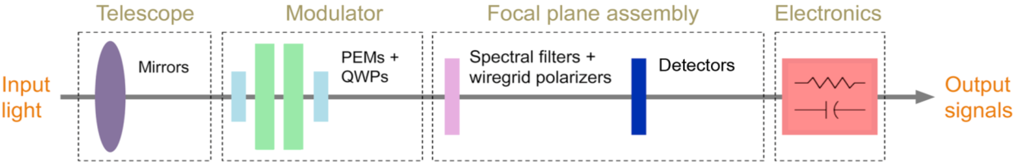
u = U/I are independent of system transmittance and detector gain variations. A schematic of the MSPI optical and detection system is shown in
Figure 1.
Figure 1.
The main elements of the Multiangle SpectroPolarimetric Imager (MSPI) polarimetric imaging approach are the telescope, the dual- photoelastic modulator (PEM) retardance modulator, the focal plane assembly, and electronics.
Figure 1.
The main elements of the Multiangle SpectroPolarimetric Imager (MSPI) polarimetric imaging approach are the telescope, the dual- photoelastic modulator (PEM) retardance modulator, the focal plane assembly, and electronics.
Results from our first prototype camera, LabMSPI, are described in [
24]. LabMSPI was a single wavelength (660 nm) camera designed to demonstrate the dual-PEM imaging concept. This instrument has since been upgraded to multispectral operation and renamed GroundMSPI to distinguish it from its predecessor. A second, airborne version of the camera—AirMSPI—has since been built, and has been flying on NASA’s ER-2 high-altitude aircraft since 2010 [
29].
2.2. Telescope Optics and Retardance Modulator
The GroundMSPI telescope is a three-mirror f/5.6 anastigmatic and telecentric system with an effective focal length (EFL) of 29 mm. The camera body and mirrors are the same ones used in LabMSPI as they were originally designed with multispectral operation in mind. The system is capable of imaging over a ±31° cross-track field of view (FOV), but only the central ±15° is used because the prototype detector array is limited in length. The three mirrors were coated with high-performance thin films to minimize diattenuation (absolute difference divided by the sum of reflectance for light polarized in planes perpendicular and parallel to the plane containing the incident and reflected light) [
30]. Reflectance varies from mirror to mirror, with a worst-case performance of 50% reflectance in the ultraviolet for the second mirror, increasing to >90% at longer wavelengths.
The PEMs used in GroundMSPI are Hinds Instruments Series II/FS42 devices, with resonant frequencies of f1 = 42,060 and f2 = 42,033 Hz at 20 °C. These frequencies shift by about 1.9 Hz per 1 °C change in temperature, but the difference frequency Δf = f1 – f2 (27 Hz) is much less temperature sensitive, changing by only 17 mHz per °C. The fast axes of the PEMs are aligned and nominally parallel to the long dimension of the focal plane line arrays. The small difference in resonant frequency of the two PEMs generates a beat signal whose period defines the duration of an image frame (tframe = 1/Δf). In a spaceborne application, the 37 ms frame time would yield a similar spatial resolution and sample spacing as MISR. The detectors are read out many times during each frame (i.e., every few ms) in order to sample the modulation pattern.
For the dual-PEM system to modulate both Q and U, the PEMs are preceded and followed by QWPs with their fast axes at 45° to the fast axes of the two PEMs. When a linearly polarized beam is incident on the resulting circular retarder, the orientation of the linearly polarized exiting beam rotates clockwise and counterclockwise as the PEMs oscillate, leading to a modulated signal when viewed through a polarization analyzer. In the single-band LabMSPI camera, zero-order quartz QWPs were used. For GroundMSPI, these were replaced with commercial QWPs (supplier: Red Optronics) constructed from quartz and MgF2. Retardance is within 8° of quarter wave at 470, 660, and 865 nm. The departure from ideal performance is compensated in calibration.
2.3. Focal Plane Spectropolarimetric Filters
To provide spectral and polarimetric selection for different rows of the photodetector line arrays, the GroundMSPI spectral filters were sliced to a long, narrow geometry (80 µm wide for each channel by 17 mm long), bonded together, and polished. The filter assembly is positioned in the camera focal plane just ahead of the detector array. The spectral filter assembly was bonded to a thick substrate containing patterned wire-grid polarizers (WGPs) in those channels for which polarization data are obtained. Barr Associates, Inc. (now Materion Barr Precision Optics) designed and fabricated the stripe filters and Moxtek, Inc. supplied the patterned polarizers. Cross-coupling between Q and U signals due to ghosting is minimized by maximizing the distance between the WGP and the anti-reflection (AR) coated surface of the filter. High optical density black epoxy is used between the spectral filters for stray light reduction.
GroundMSPI spectral bands are centered at 355, 380, 445, 470P, 555, 660P, 865P, and 935 nm. Those marked with the letter “P” are polarimetric. Full width at half maximum bandpasses are 29, 33, 38, 39, 29, 39, 38, and 50 nm, respectively. Measurements of Moxtek WGPs before lamination to the filters showed transmissions in the range 85–90% and extinction ratios (ratio of transmittance of the polarization state aligned with polarizer to the transmittance for the orthogonal state) in the range of hundreds to thousands, with better performance in the red and near-infrared than in the blue. Application of a cement bond to the WGPs changes the refractive index between the wires, resulting in reduced transmittance and polarization extinction ratio. However, the use of high-contrast WGP stock results in post-bond transmittance exceeding 75% and extinction ratios between 40 and 100, depending on wavelength. A lower extinction ratio simply reduces the magnitude of the modulation pattern from the PEMs, and is readily dealt with in instrument calibration.
Some imperfections in the GroundMSPI filters occurred during the manufacturing process. The most notable defect was the failure of a dark mask to be completely removed from the intended area of light transmission for about 40% of the width of the 555-nm channel, resulting in much lower than desired throughput. However, because the filter passes some light, flat-field calibration is able to compensate for this defect.
2.4. Focal Plane Detectors
The complementary metal oxide semiconductor (CMOS) silicon line array detectors used in GroundMSPI cover the ultraviolet (UV) to visible/near-infrared (VNIR) spectral range. Sixty-four lines on 16 µm spacing contain 1,536 pixels with 9.5 µm (cross-track) × 10 µm (along-track) apertures. A first-generation detector array was fabricated by Tower Semiconductor, Ltd. This chip (designated MSPI-1) was used in LabMSPI but readout speeds were not fast enough for GroundMSPI due to the presence of parasitic capacitances. The MSPI-1 chip reached noise levels that rendered it unusable at speeds exceeding 12.5 MHz. Consequently, the chip design was updated and second-generation detectors, designated MSPI-2A and MSPI-2B (distinguished by their different conversion gains), were procured from Tower. Increased conversion gain reduced the noise floor from 26 e− for MSPI-1 to 18 e− for MSPI-2A and 9 e− for MSPI-2B. The latter design is used in GroundMSPI. Dark current was measured at 0.5 e−·s−1. Quantum efficiency was determined to be about 35% at 660 nm.
2.5. Electronics
Electronic circuits were designed and built to meet dual-PEM polarimeter signal timing and phasing requirements in accordance with specifications outlined in [
23]. That paper demonstrated that polarimetric accuracy is maximized by properly sampling the video signal and by synchronizing the sampling with the retardance modulation of the dual PEM. To accomplish these objectives, the GroundMSPI support electronics are divided between a Focal Plane Array (FPA) board and a Data Recovery Board (DRB). Both boards have their operation controlled by a set of programmable registers. The FPA contains the detector array and provides the low-level analog and digital signals needed to operate it. It also captures the output data and sends it, along with appropriate sync signals, to the DRB over a CameraLink interface. Digital signals are generated by a Xilinx Spartan-3 field programmable gate array (FPGA) operating at 50 MHz, while the analog ramp is generated by a 16-bit Analog Devices digital-to-analog converter (DAC). The ramp is divided into 512 steps, and programmable to keep quantization noise smaller than shot noise. The DRB, also based on a Spartan-3 FPGA, performs two functions. First, it generates the signals needed by the FPA board to synchronize it to the high and low frequency modulations. Second, it performs the subtraction needed to implement correlated double sampling (CDS), which is used to minimize noise resulting from resets of the detectors that occur each integration interval. The DRB receives synchronization signals from the two PEM controllers, each of which drives an all-digital phase locked loop. Data from the camera are acquired using a fast IOindustries CL-160 CameraLink frame grabber.
2.6. Calibration
Radiometric and polarimetric calibration are important for using GroundMSPI data quantitatively. The camera’s radiometric transfer curve (relationship between illumination and digital output) is established in the laboratory by using the MISR 1.65 m integrating sphere as the illumination source. The integrating sphere also provides the illumination for determination of the pixel-by-pixel gain coefficients. Independent measurements of the sphere intensity are obtained from a 670-nm photodiode radiance standard, calibrated against a NIST traceable incandescent lamp (Optronics OL 220C, SN: M-1188), and a Photo Research PR-650 scanning spectrophotometer. Offset levels to account for pixel-by-pixel variations in dark current are obtained by acquiring data in the dark.
Polarimetric calibration compensates for instrumental polarization. A laboratory polarization state generator (PSG) was constructed for this purpose. Illumination from light-emitting diodes (LEDs) is depolarized, collimated, and transmitted through a high-extinction polarizer (DOLP = 1.000) to provide a source of fully polarized light. Because of the great care taken in controlling instrument polarization, the GroundMSPI camera operates as an imaging polarimeter with high DOLP accuracy even prior to calibration; however, refinement is necessary to meet the specification of DOLP uncertainty <±0.005. Rotation of the high-extinction polarizer in 10° steps provides the necessary observations to determine polarization calibration coefficients on a pixel-by-pixel basis. Once these coefficients are known, the calibrated normalized Stokes parameters are determined according to the procedure described in [
24].
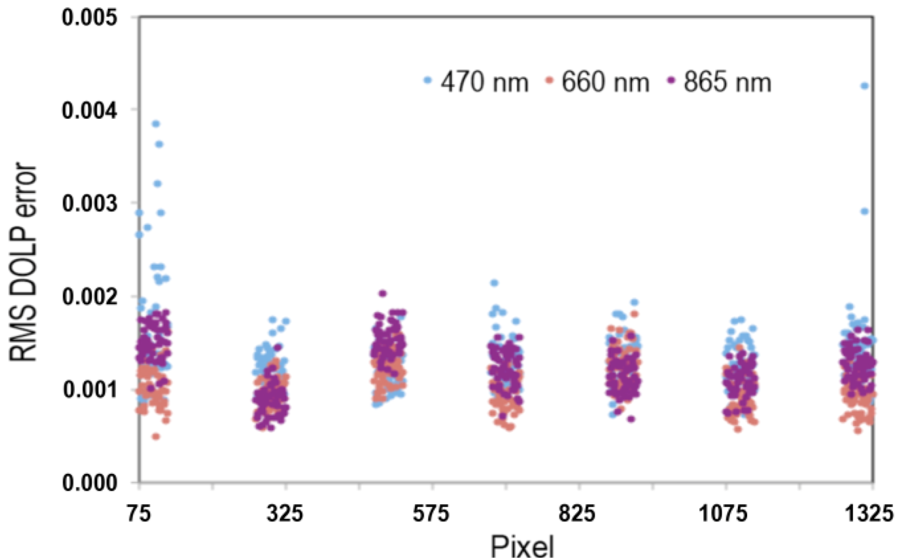
Figure 2.
Root-mean-squared (RMS) error in degree of linear polarization (DOLP), calculated as deviations from 1.000 as a high-extinction polarizer is rotated in 10° steps in front of the GroundMSPI camera. Polarimetric calibration is done in segments, since the light-emitting diode (LED) illumination covers only a portion of the camera field of view (FOV). Results from seven segments across the FOV are shown here.
One measure of the uncertainty in DOLP is the root-mean-squared (RMS) fluctuation in calibrated DOLP as the input orientation of the high-extinction polarizer is varied. Illustrative results from the GroundMSPI camera are shown in
Figure 2. The LED illumination spot used in polarimetric calibration illuminates only short segments of the line arrays at a given time, and the camera is rotated cross-track to span the whole array.
Figure 2 shows residual DOLP error for seven segments of the line arrays at 470, 660, and 865 nm. With the exception of a few pixels near either end of the focal plane, RMS DOLP error is typically <0.002, and the 0.005 specification is met even for the outlier pixels.
3. GroundMSPI Imagery
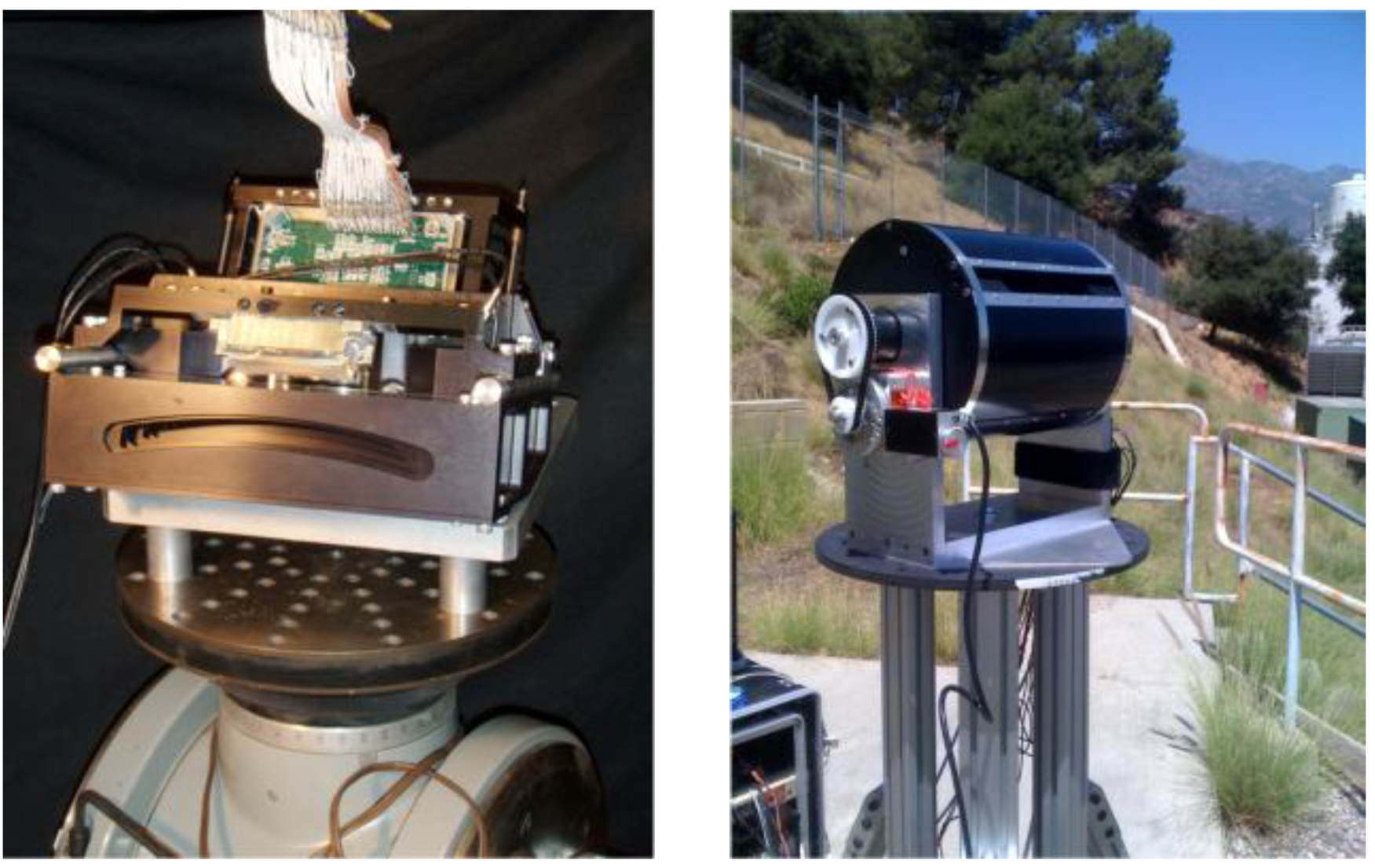
As GroundMSPI is a pushbroom camera, two-dimensional imagery of landscapes and skyscapes is acquired by mounting the camera in a drum and rotating the field of view about a horizontal axis. The gimbal is driven by a commercial micro-stepper rotary stage (Aerotech ART100) and scanned vertically from below the horizon toward the zenith at a rate of 0.5° s
−1. The GroundMSPI camera and drum are shown in
Figure 3. The data processing system for GroundMSPI builds upon heritage from the MISR and AirMISR projects [
31,
32]. Conversion of raw camera outputs to imagery takes place in several steps. Level 1A1 reformats the raw GroundMSPI output into Hierarchical Data Format (HDF). Level 1A2 performs data conditioning such as compensation for detector nonlinearity and dark level subtraction. Level 1B1 extracts the Stokes parameters
I,
Q, and
U and their linear gradients during each image frame, and applies pixel-by-pixel radiometric gain coefficients. Level 1B2 spatially co-registers the channels and corrects for residual instrument polarization, and derives DOLP and AOLP.
Figure 3.
The Ground-based Multiangle SpectroPolarimetric Imager (GroundMSPI) camera (left) is mounted in a rotating drum (right) to provide pushbroom imagery of landscapes.
Figure 3.
The Ground-based Multiangle SpectroPolarimetric Imager (GroundMSPI) camera (left) is mounted in a rotating drum (right) to provide pushbroom imagery of landscapes.
At a target distance of 100 m, the GroundMSPI spatial resolution is 3 cm and the scene width is about 50 m. These parameters scale linearly with distance to the target.
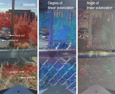
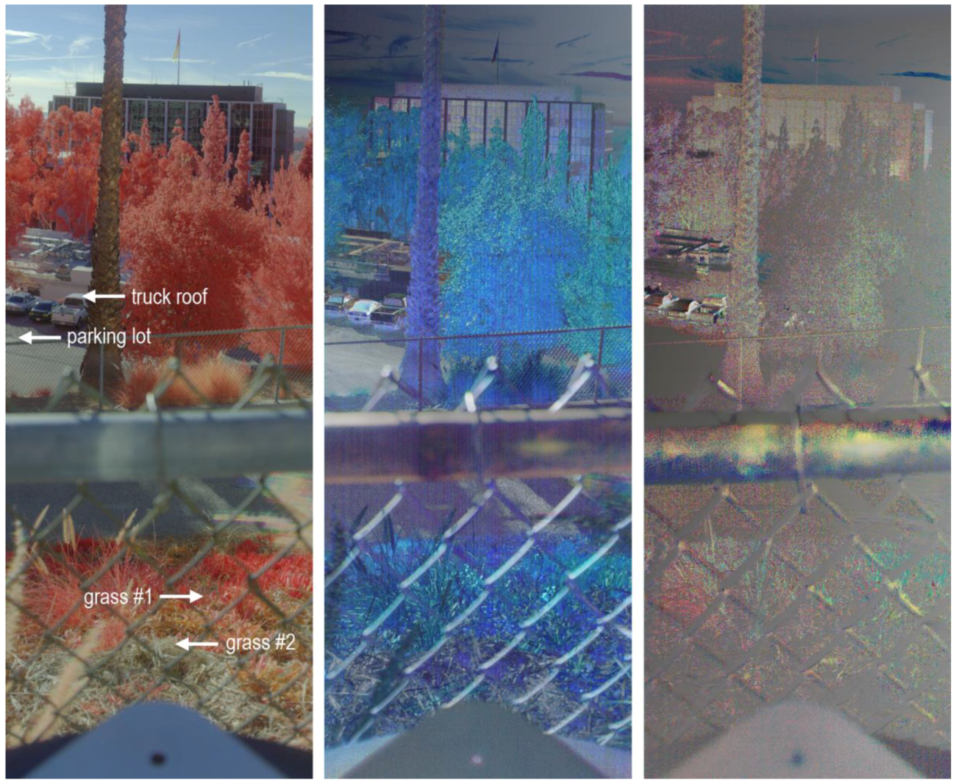
Figure 4 shows example data from the 470, 660, and 865 nm bands, acquired at JPL on 6 January 2010 at 8:44 am PST (1644Z), viewing toward the south-southeast. The parameters displayed are intensity, DOLP, and AOLP, the latter defined with respect to the scattering plane,
i.e., the plane containing a line from the target to the Sun and a line from the target to the camera. A portion of the plate upon which the camera is mounted is visible at the bottom of each image (also visible in right hand photograph in
Figure 3).
Four targets are identified within the GroundMSPI imagery: a patch of grass (#1) viewed at a zenith angle θ of 63°, a second patch of grass (#2; θ = 59°) with smaller near-infrared reflectance, a small area within the parking lot (θ = 83°), and a truck roof (θ = 86°). Multiangle data were acquired by collecting images at varying solar zenith angles throughout the day as the Sun traversed the sky. Images were acquired hourly at 8:44 am, 9:44 am, 10:43 am, 11:44 am, 12:45 pm, 1:44 pm, 2:44 pm, and 3:44 pm, corresponding to solar zenith angles of 73°, 65°, 59°, 57°, 58°, 62°, 69°, and 78°, respectively. The observational data from these targets are compared to the predictions of a surface reflection model that accounts for both intensity and polarization. The model is described in the next section.
Figure 4.
Example GroundMSPI imagery from 6 January 2010. From left to right: Intensity, DOLP, and AOLP at 470, 660, 865 nm displayed as blue, green, and red.
Figure 4.
Example GroundMSPI imagery from 6 January 2010. From left to right: Intensity, DOLP, and AOLP at 470, 660, 865 nm displayed as blue, green, and red.
4. Surface Reflection Model
We established a polarized bidirectional reflectance distribution function (PBRDF) represented by a Mueller matrix describing both intensity and polarization [
33], and followed the practice of representing the PBRDF as the sum of a depolarizing volumetric scattering term and a polarizing reflection term [
18,
34,
35]. The modified Rahman-Pinty-Verstraete (mRPV) function [
36] is used for the volumetric term. Litvinov
et al. [
18] used the original RPV function [
37], but the modified form, used in MISR retrievals, has the advantage that it is linearizable in its parameters by taking the natural logarithm. For simplicity, we have ignored the hotspot factor, which is significant only near the direct backscatter direction. Following common practice, a distribution of tilted microfacets models the polarized reflection. Then, the PBRDF f
λ at wavelength λ is written in matrix form as:
where
Letting θ = view zenith angle, θ
0 = solar zenith angle, μ = cosθ, μ
0 = cosθ
0, φ = view azimuth angle, and φ
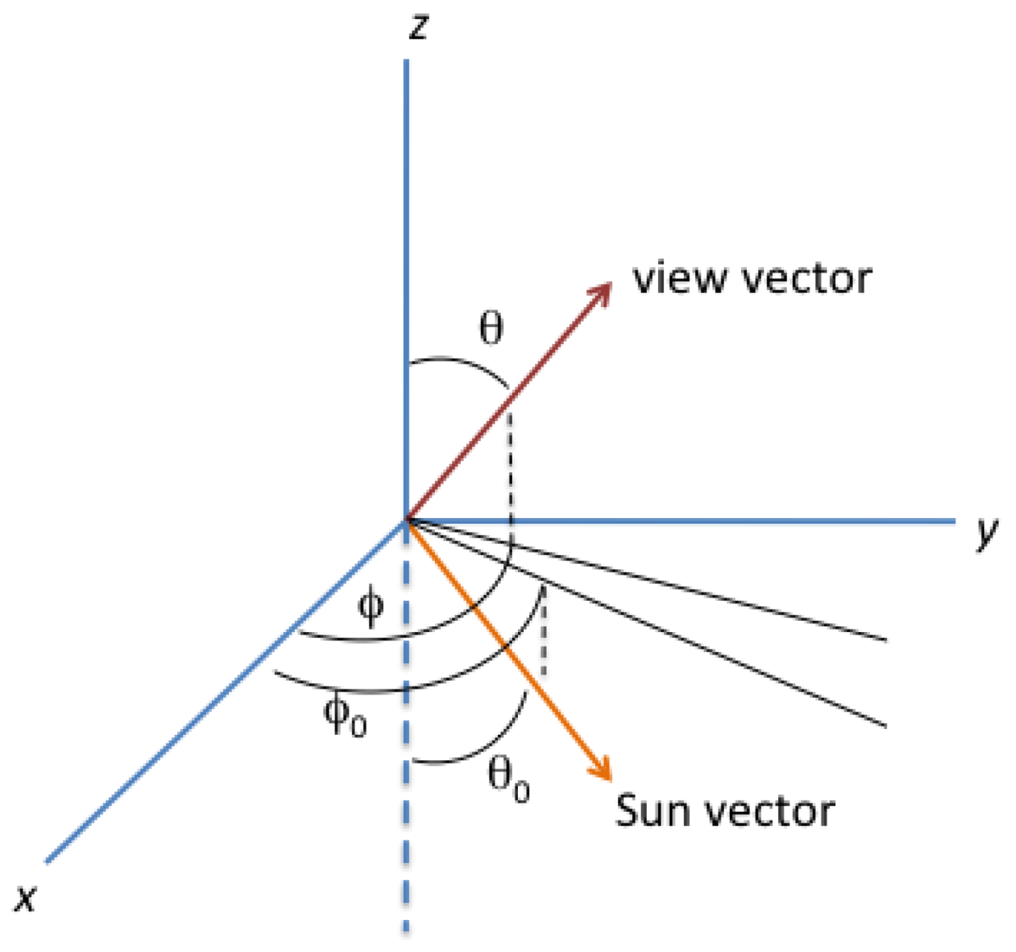
0 = solar azimuth angle, we define the Sun and view vectors as pointing in the direction of photon travel (see
Figure 5). The scattering angle Ω between these vectors is:
Figure 5.
Sun and view vectors in a coordinate system with z-axis normal to the Earth’s surface.
Figure 5.
Sun and view vectors in a coordinate system with z-axis normal to the Earth’s surface.
The mRPV function is an empirical parameterization of unpolarized surface reflectance that accounts for volumetric scattering within the surface medium. It is written here as the product of a function only of wavelength and a function only of illumination and view geometry, and is described by the parameters
aλ,
k, and
b, the latter two assumed to be spectrally invariant. A Lambertian model would have
k = 1 and
b = 0. The depolarization matrix D in Equation (6) is a Mueller matrix with unity in the upper left-hand element and zeros everywhere else (
i.e., only an unpolarized intensity field is reflected, regardless of the polarization state of the illuminating light) [
38].
The second component of the PBRDF assumes that the surface is made up of an array of tilted microfacets, such that for a given illumination and view geometry some fraction of the facets have the appropriate orientation to specularly reflect sunlight into the sensor. The microfacet concept has a long history of use in the intensity domain for modeling the reflection from roughened surfaces, e.g., [
34,
39], and has been used to achieve photorealistic rendering in computer graphics, e.g., [
40,
41]. Microfacet models have more recently been extended into the polarization domain [
42]. Generalizing the work of Bréon [
43], who derived the scalar BRDF, and the polarized formulation by Priest and Meier [
42], we represent the PBRDF for a distribution of facets by:
where we have introduced a wavelength-independent scaling parameter ζ multiplying the polarized surface reflectance matrix. P is the Mueller matrix for reflection by each facet within the facet coordinate system, and rotations between the global and facet coordinate systems are represented by the matrices M(α
0) and M(−α), where α
0 and α are the angles between the scattering plane and the solar and view meridian planes, respectively. The solar meridian plane contains the global horizontal surface normal (
i.e., the
z-axis in
Figure 5) and the Sun vector, and the view meridian plane contains the global horizontal surface normal and the view vector. When these two planes coincide, the result is known as the principal plane. With the assumption that the complex refractive index of the surface is spectrally neutral, we do not include a wavelength subscript on P.
For a surface height
z that is a function of position
x and
y, we let
p'(
zx,
zy) represent the probability density that a facet has an orientation with
zx and
zy in the intervals
zx±dzx/2 and
zy±dzy/2, where
zx is the partial derivative of
z with respect to
x, and
zy is the partial derivative of
z with respect to
y. The facet tilt angle β (the angle between the global horizontal surface normal and the facet normal) is related to
zx and
zy by
![Atmosphere 03 00591 i013]()
. According to the law of reflection, the facet normal vector lies in the plane defined by the Sun position vector and the view vector. It is convenient to transform from a facet orientation probability density in
zx,
zy space to polar coordinates β, ψ because the analytic probability density functions we will use are azimuth (ψ) independent. In this case
zx = tanβcosψ and
zy = tanβsinψ. We note that when integrating over all possible facet orientations, the probability distributions are normalized such that:
where
dω = sinβ
dβ
dψ is an element of solid angle. The transformation of coordinates makes use of the Jacobian determinant, such that:
in which the Jacobian determinant is given by
Since
dcosβ
dψ = −sinβ
dβ
dψ,
Assuming azimuthal symmetry of the facet orientation distribution, the total surface PBRDF is
Examples of facet distributions are the uniform distribution, the Bréon
et al. model [
19], and the Gaussian model [
39,
44]:
The uniform and Bréon
et al. models are the lowest order (
m = 0, 1) examples of the Stryjewski
et al. [
45] normalization of the Blinn-Phong facet distribution [
40,
46],
p = (
m + 1)cos
mβ/2π. For the Gaussian distribution an additional parameter, the slope variance σ
2, is included. This model was used by Cox and Munk [
39] to model the rough ocean surface, but the same model can also be applied to solid surfaces. For example, a Gaussian microfacet model was used in the laboratory to interpret passive multiangle polarimetry and determine the complex refractive index of various materials [
47].
In the simplest form of the microfacet model, the single reflection from each facet is governed by the Mueller matrix for Fresnel reflection F(γ,
nr,surf,
ni,surf), where γ is the angle of incidence and reflectance for specular reflection from the surface of a facet and
nsurf =
nr,surf−
ini,surf is the complex refractive index. This matrix is defined in the local coordinate system of a facet, and is written as
where
Data from airborne polarimeters suggest that
nr,surf = 1.5 and
ni,surf = 0 work reasonably well for natural targets [
20]. The factor ζ in Equation (13) compensates for a possibly incorrect choice of
nr,surf [
21]. There are only four unique elements in F, each of which is a function of the Fresnel coefficients. From Bohren and Clothiaux [
48], the Fresnel reflection coefficients for the electric field components parallel (
p) and perpendicular (
s) to the scattering plane are
where γ is defined above and γ' is the angle of transmission for the refracted light. Assuming a refractive index of unity for the illuminating medium,
nsurfsinγ' = sinγ from Snel’s law, where γ' is a complex number if
nsurf is complex. Hence
rp and
rs are in general complex. Then [
48],
where the asterisk denotes the complex conjugate.
In Equation (13), rotations between the global and facet coordinate systems are represented by the matrices M(α
0) and M(−α), where
By performing the appropriate rotational transformations, we derive the following expressions:
which are mathematically equivalent to formulas given in [
42] and [
49].
From the definition of PBRDF, the reflected Stokes vector from the surface is given by
where
E0λ is the exo-atmospheric spectral solar irradiance at the standard Earth-Sun distance of 1 AU,
RES is the actual distance to the Sun (in AU) at the time of observations, and τ
λ is the atmospheric optical depth due to the combination of Rayleigh and aerosol scattering (although the latter is ignored in this study). L
diffinc is the Stokes vector of the incident downwelling diffuse radiation field, and takes into account multiple reflections between the surface and the bottom of the atmosphere.
5. Analysis of the GroundMSPI Observations
In using GroundMSPI to evaluate the surface model, we use data acquired on a clear day and assume negligible atmospheric extinction between the sensor and surface target. We model the surface illumination as due to the attenuated solar beam and diffuse skylight from a standard Rayleigh scattering atmosphere at sea level. Independent measurements of aerosol optical depth (AOD) were not available, but the conclusions presented below are not especially sensitive to AOD. Exo-atmospheric solar irradiances were obtained from Wehrli [
50], and corrected for the actual distance to the Sun (
RES = 0.983 AU) on the date the data were acquired. The following atmospherically-corrected bidirectional reflectance factors (BRFs) are defined:
The direct-field
I,
Q, and
U are obtained by subtracting the values corresponding to reflection of diffuse skylight from the observations. The latter are obtained from the modeling, described below.
Much of the remote sensing literature concerned with development and testing of polarized surface reflectance models, e.g., [
51,
52,
53] focuses on the polarized surface bidirectional reflectance factor
BRPF; that is, the Stokes parameters
Q and
U are usually not considered individually. An exception is Litvinov
et al. [
18], who tested the measured ratio
Q/U from airborne polarimeter observations against theoretical expectations from a single-bounce microfacet model and found reasonable agreement for soil and vegetation samples. In this paper, we fit
Ipol from the GroundMSPI observations, and then decompose the model into its implied
Q and
U components as a check of physical fidelity. Direct fitting of
Q and
U is also explored. The investigation proceeds in five steps. In step 1, only direct solar illumination of the surface is considered. In step 2, illumination by diffuse skylight is incorporated into the calculations. Step 3 improves the fits to
I and
Ipol by using the observations to empirically constrain the angular variation of the reflection of direct sunlight, assuming spectral invariance in the angular shape of
BRF and
BRPF and retaining the analytic components of Equation (13) as the boundary condition for diffuse illumination. Although this improves the fit to the observed
Ipol considerably, it does not guarantee that the modeled values of
Q and
U individually match the measurements. We then show in steps 4 and 5 how generalization of the facet Mueller matrix leads to improvements to the fits to
Q and
U. In step 4, we relax the assumption that the
P31 component of the facet Mueller matrix is identically zero, as implied by the Fresnel model (Equation (15)). In step 5, a physical model for the Mueller matrix governing reflection of direct sunlight is abandoned, and replaced by empirically determined functions for
BRQF and
BRUF, assuming spectral invariance in their angular shapes.
In the following discussion, the values of
Q and
U obtained from the GroundMSPI data are defined with respect to the view meridian plane. This convention is chosen for consistency with the matrix rotations in Equation (13), and is different than the convention used in the AOLP image of
Figure 4, where the reference orientation was taken as the scattering plane. Thus, while
U = 0 for a single reflection of unpolarized light within the local coordinate system of an individual microfacet, transformation to the view meridian plane rotates the linear Stokes vector components such that
U is in general non-zero.
5.1. Consideration of Direct Solar Illumination Only (Step 1)
In Step 1, illumination by diffuse skylight is ignored, and the data are modeled by just the first term of Equation (22). This simple form of the model is entirely analytic. Because the target illumination is dominated by attenuated direct sunlight, the results of this step provide a useful reference with which to gauge additional model complexities. There are 6 surface model parameters to solve for, the three spectral values of aλ, plus k, b, and ζ. Because specular reflection from the facets contributes to the total radiance field as well as the polarized field, it is convenient to solve for ζ first, as the polarized field is unaffected by aλ, k, and b. A simple least-squares fit is used to minimize the residual between the measured and modeled polarized radiances, assuming a uniform facet distribution and incorporating information from all three wavelengths simultaneously in performing the fit. Then, the specularly reflected term is subtracted from the measured radiances to solve for aλ, k, and b. Because the natural logarithm of the direct field radiance (minus the specular term) is linear in log aλ, k−1, and b, linear least squares fitting is used to solve for these parameters.
The derived numerical values for the parameters are shown in
Table 1. Because the
aλ,
k, and
b parameters are not orthogonal, the retrieved values are not necessarily unique. This may account for the low values of
aλ and high value of
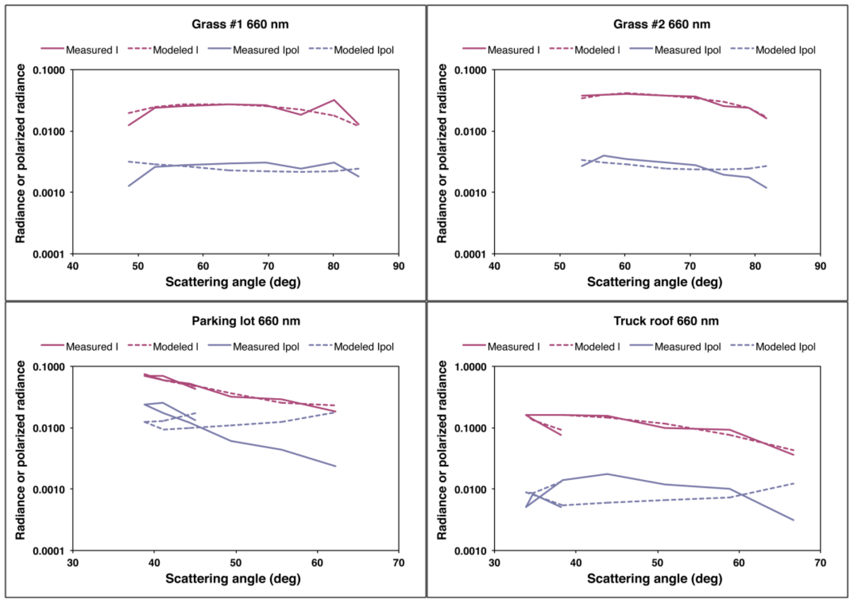
b obtained for the parking lot. Nevertheless, this set of parameters provides reasonably good fits to the intensity data. Graphical results at 660 nm are shown in
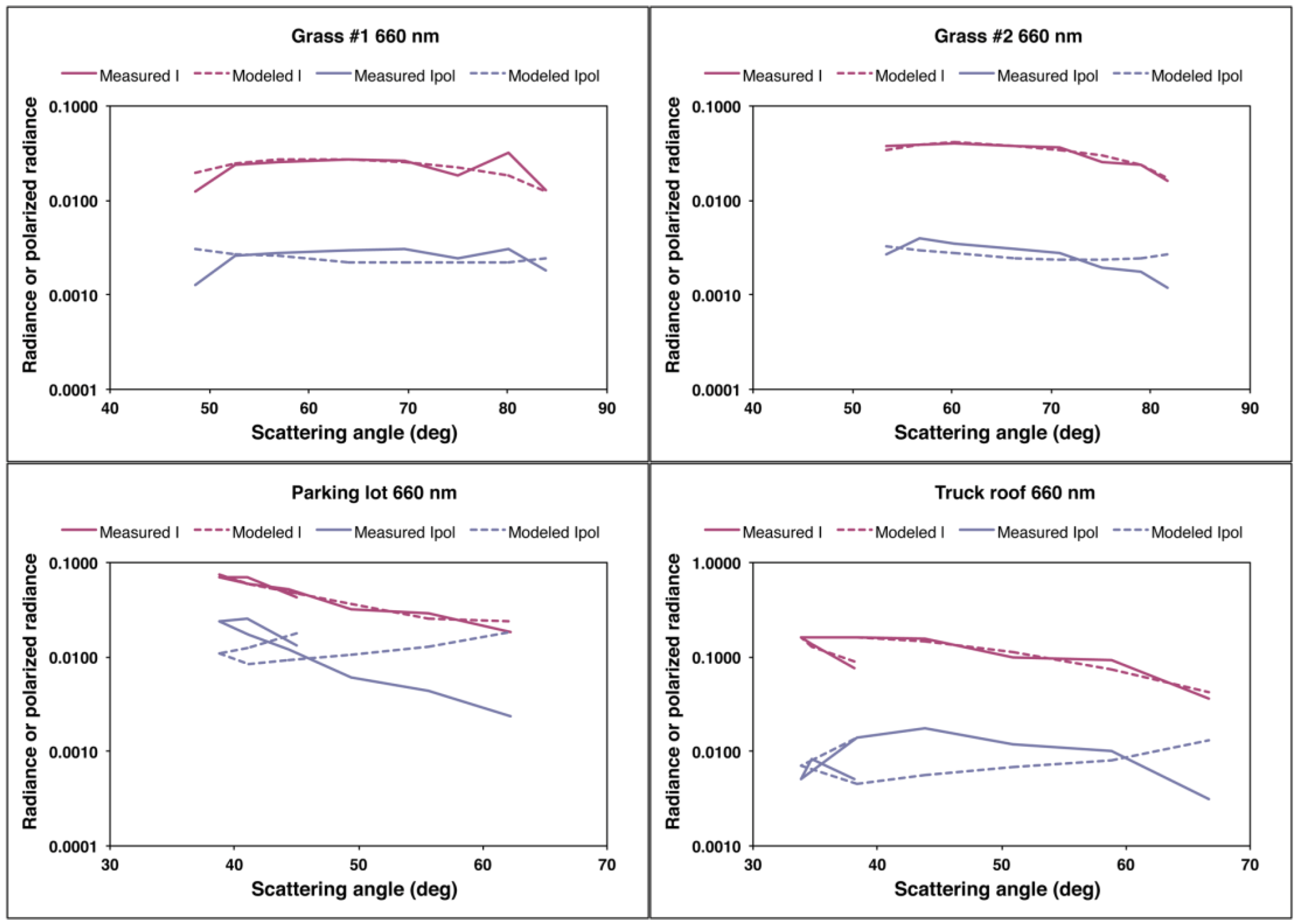
Figure 6; the results at 470 nm and 865 nm show similar patterns. While total intensity is fitted well for all targets, the model matches the polarized intensity for only the grass targets. Other analytic facet distribution functions, e.g., Bréon and Gaussian, do not significantly improve the fits. The
Q and
U components are derived by assuming that the facet Mueller matrix P is described by the Fresnel model such that the factors
sign(
P21)cos2α and −
sign(
P21)sin2α, respectively, multiply the directly illuminated component of
Ipol to obtain
Q and
U. The
sign(
P21) factor is included to ensure the proper sign of the results. The results are illustrated in
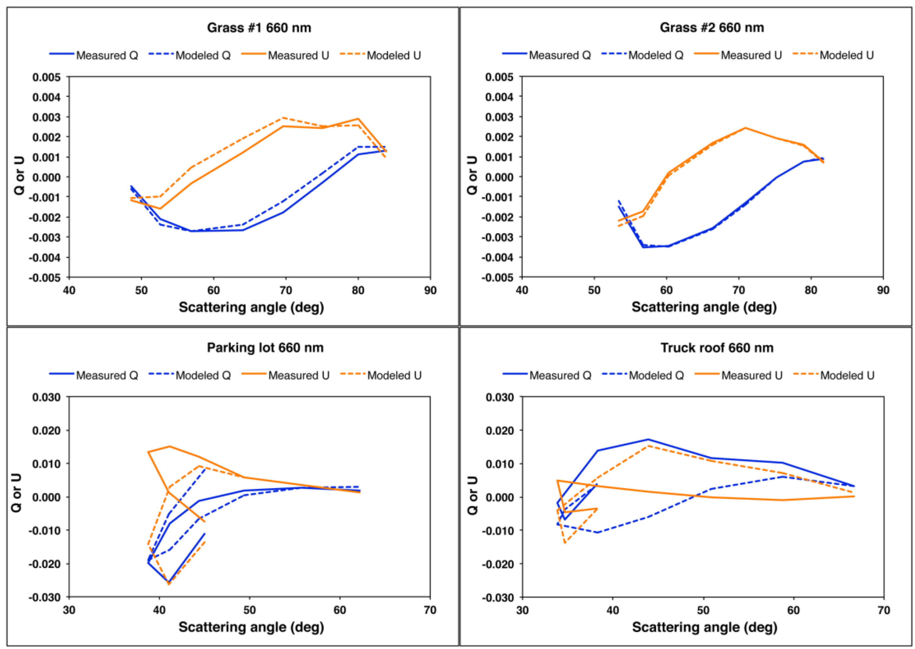
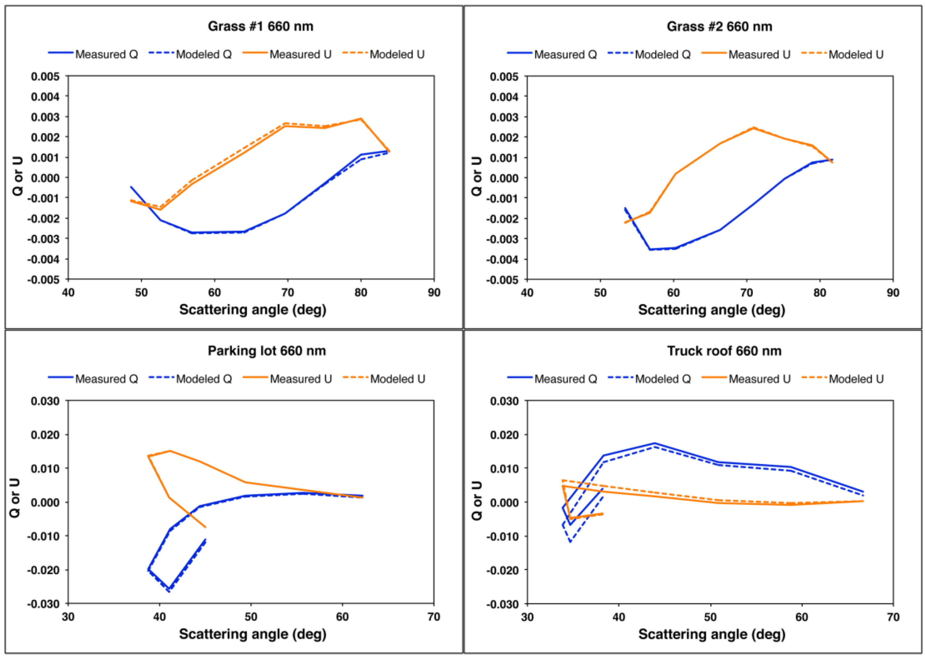
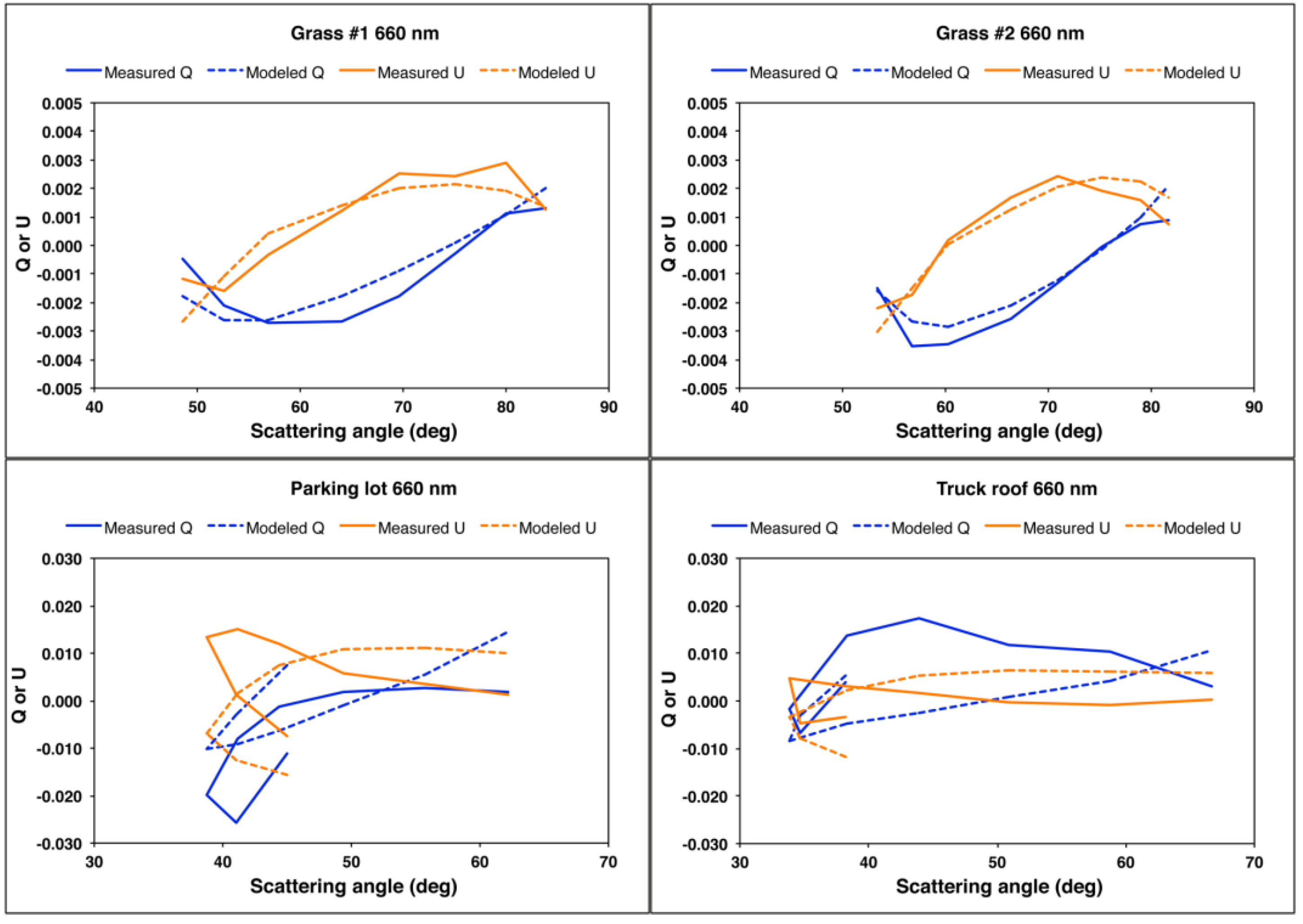
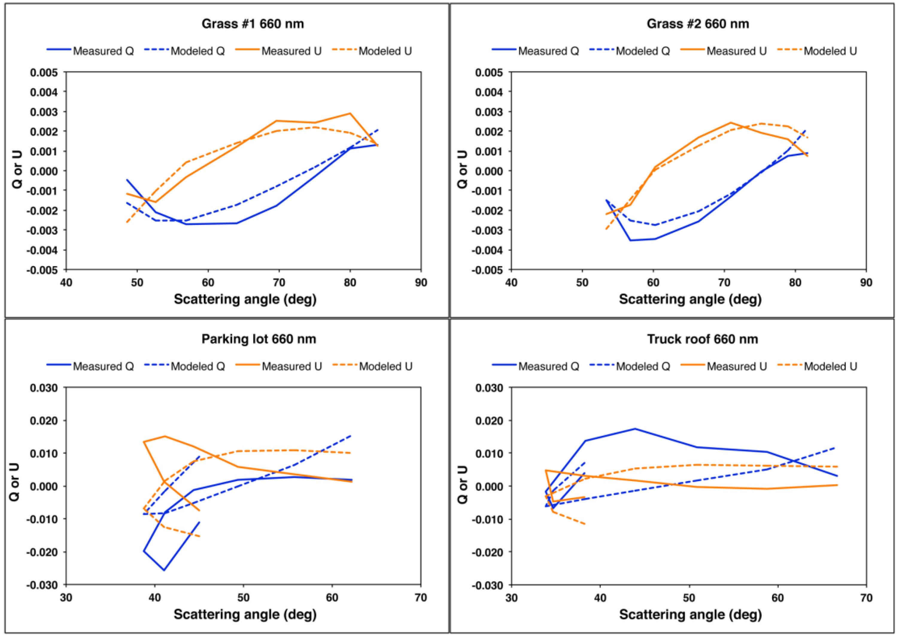
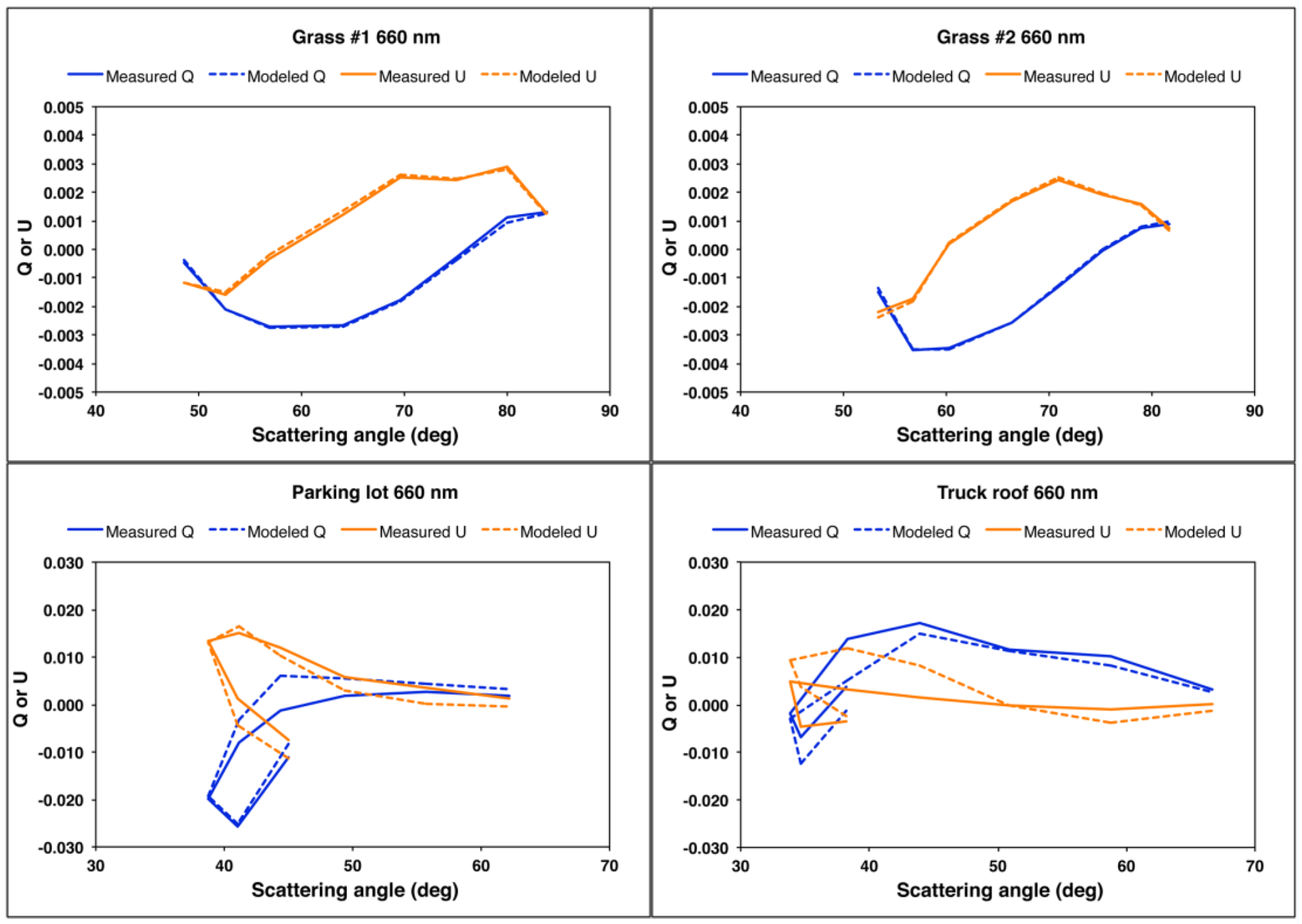
Figure 7, which shows measured and modeled
Q and
U vs. scattering angle at 660 nm. For the grass targets, the relative variation with scattering angle, the signs of
Q and
U, and their relative magnitudes are correctly predicted. However, the model is unsuccessful for the parking lot and truck roof. Modifications to the model that affect
Q and
U identically, such as a different facet orientation distribution function, or inclusion of a shadowing term, would simply scale
Q and
U and would not improve the fits.
Table 1.
Fitted model parameters during Steps 1 and 2 of the fitting process.
Table 1.
Fitted model parameters during Steps 1 and 2 of the fitting process.
| Target | Step | a470 | a660 | a865 | k | b | ζ |
|---|
| Grass #1 | 1 | 0.035 | 0.063 | 0.308 | 0.818 | 0.385 | 0.212 |
| 2 | 0.028 | 0.060 | 0.307 | 0.833 | 0.408 | 0.203 |
| Grass #2 | 1 | 0.031 | 0.057 | 0.108 | 0.657 | 1.127 | 0.276 |
| 2 | 0.026 | 0.055 | 0108 | 0.676 | 1.167 | 0.262 |
| Parking lot | 1 | 0.0009 | 0.0010 | 0.0012 | 0.701 | 5.754 | 0.161 |
| 2 | 0.0005 | 0.0007 | 0.0008 | 0.761 | 6.642 | 0.153 |
| Truck roof | 1 | 0.338 | 0.275 | 0.297 | 1.030 | 1.114 | 0.046 |
| 2 | 0.327 | 0.299 | 0.333 | 1.090 | 1.272 | 0.043 |
Figure 6.
Total and polarized radiances measured by GroundMSPI at 660 nm as a function of scattering angle for the four targets identified in
Figure 4 (solid lines), along with fitted values from Step 1 (dashed lines) using the first term of Equation (22) and the uniform facet distribution.
Figure 6.
Total and polarized radiances measured by GroundMSPI at 660 nm as a function of scattering angle for the four targets identified in
Figure 4 (solid lines), along with fitted values from Step 1 (dashed lines) using the first term of Equation (22) and the uniform facet distribution.
Figure 7.
Q and
U measured by GroundMSPI at 660 nm as a function of scattering angle for the four targets identified in
Figure 4 (solid lines), along with values implied by the model for
Ipol derived in Step 1 of the modeling (dashed lines).
Figure 7.
Q and
U measured by GroundMSPI at 660 nm as a function of scattering angle for the four targets identified in
Figure 4 (solid lines), along with values implied by the model for
Ipol derived in Step 1 of the modeling (dashed lines).
5.2. Inclusion of Diffuse Skylight (Step 2)
In an attempt to explain the deviations of the parking lot and truck roof data from the simple model, the next level of complexity was inclusion of diffuse skylight,
i.e., the second term on the right hand side of Equation (22). Reflection of polarized skylight has the potential to modify the observed values of
Q in all azimuthal planes, and to modify
U provided that the observations are off the principal plane such that the distribution of sky polarization is not symmetric. To include reflection of skylight in the scene model, the surface PBRDF was incorporated into a Markov chain vector radiative transfer code [
54]. In this method, the atmosphere is divided into
N layers and the light propagation direction within the atmosphere is discretized into a finite number of angles. After a Fourier series expansion in the difference between the view and incident azimuthal angles, φ − φ
0, the “state” of the radiant energy deposited in each Fourier mode is described by its vertical layer and its direction of propagation. Then the diffuse reflection matrix R
atm at the top of the atmosphere (τ = 0) and diffuse transmission matrix T
atm at the bottom of the atmosphere (τ = τ
λ) are determined via matrix operations describing the probably of a photon’s change of state from one vertical location and direction of propagation to another. The surface is incorporated as a special layer in which only reflection applies.
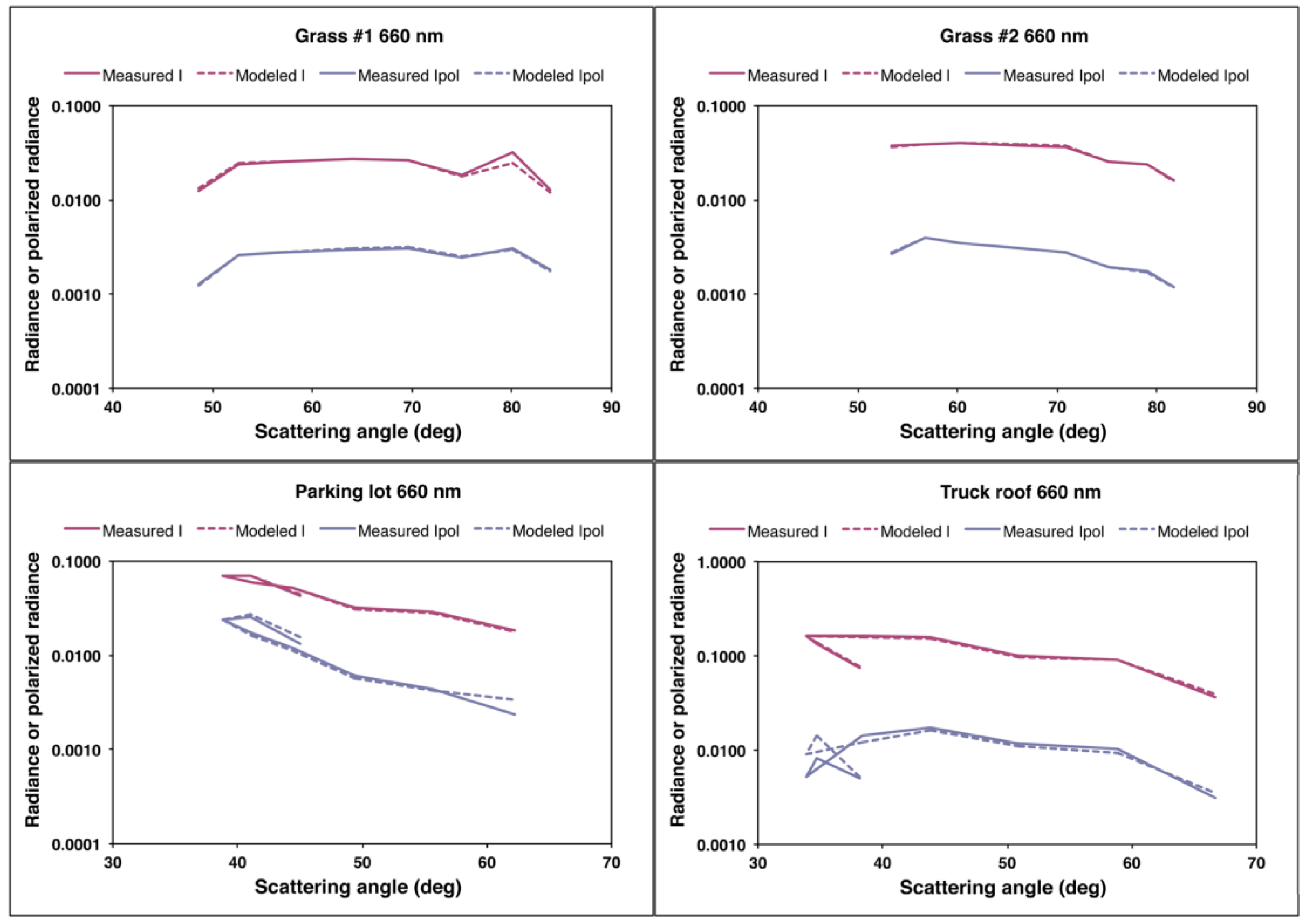
Figure 8.
Similar to
Figure 6, but for Step 2 of the modeling,
i.e., reflection of diffuse skylight (second term on right hand side of Equation (22)) is included.
Figure 8.
Similar to
Figure 6, but for Step 2 of the modeling,
i.e., reflection of diffuse skylight (second term on right hand side of Equation (22)) is included.
Figure 9.
Similar to
Figure 7, but with the modeled
Q and
U obtained from
Ipol derived in Step 2.
Figure 9.
Similar to
Figure 7, but with the modeled
Q and
U obtained from
Ipol derived in Step 2.
To solve for revised values of
aλ,
k,
b, and ζ, an iterative procedure was employed. The results from Step 1 were used as a starting guess, and the radiative transfer code was used to calculate the right hand (diffuse) term of Equation (22). This term was subtracted from the observations and the least-squares fitting procedure from Step 1 was applied to the remainder to obtain updated values of the model parameters. The diffuse-field reflection term was recalculated and this process repeated until no significant changes in the parameters were obtained. The updated values of
aλ,
k,
b, and ζ are shown in
Table 1. The similarity of the Step 2 and Step 1 values indicates that diffuse illumination does not play a major role. Indeed, the graphical form of the variations of
I,
Ipol,
Q and
U (
Figure 8 and
Figure 9) are not much different from the results in Step 1. We conclude that diffuse skylight is not the reason for the departure of
Q and
U from model predictions for the parking lot and truck roof targets.
5.3. Empirical Improvement in the Facet Probability Distribution (Step 3)
The next step was to improve the representation of
I and
Ipol as a function of scattering angle.
Figure 6 and
Figure 8 show that the analytic form of the PBRDF does not match the measured values, particularly for the manmade targets. In contrast to the randomly oriented grass stalks, the surface of the asphalt parking lot and truck roof likely violate the assumption of azimuthal isotropy in
p(β,ψ). The truck roof, in particular, contains raised ridges aligned with the long dimension of the vehicle.
To deal with this empirically, the diffuse field term derived in Step 2 is subtracted from the observed Stokes vectors, and the data are converted to
BRF and
BRPF values. We then assume that
BRF and
BRPF can each be represented as a spectrally invariant angular shape function, normalized such that its average over angle is equal to unity, multiplied by a wavelength-dependent coefficient
cλ in the case of the
BRF and a wavelength-independent coefficient ξ in the case of the
BRPF. Because the previous step provided the relative spectral scaling of the intensity
BRF, we let
cλ = Caλ. The data are converted back to intensity and polarized intensity, the diffuse terms added back in, and least-squares minimization of the difference from the observations is used to solve for the coefficients
C and ξ. The empirical angular shapes are determined by taking the atmospherically corrected
BRF and
BRPF at each wavelength, and dividing each function by its average over angle. Then, the normalized results for the three wavelengths are averaged. The resulting angular shape functions, scaled by
cλ and ξ, are used to model the direct field components of
I and
Ipol. This serves a similar purpose as the use of a shortwave infrared channel (where aerosol layers are typically more transparent) to constrain the polarized surface reflectance [
55].
The results are shown in
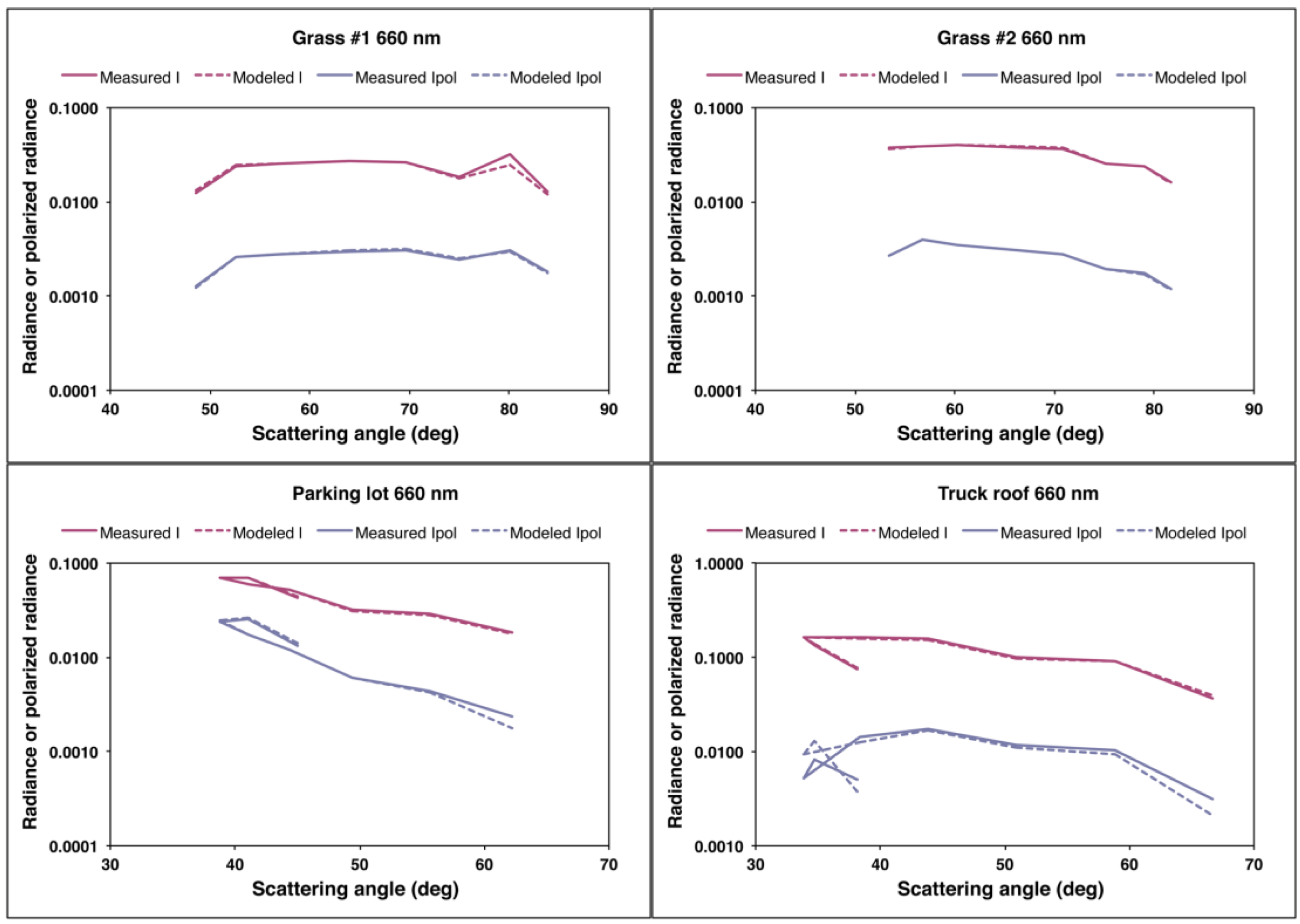
Figure 10. In comparison to
Figure 8, the modeled
I and
Ipol more closely resemble the observations. This result is contingent upon the spectral invariance in the angular shapes of
BRPF. Were the normalized shapes significantly different among the three wavelengths, the spectrally averaged shape would not be valid for any individual wavelength. In
Figure 11, the modeled
Ipol is decomposed into its
Q and
U components, as in previous steps. For the grass targets, the implied
Q and
U show improved fits to the data compared with the results obtained in Step 2. However, the
Q and
U results for the parking lot and truck roof targets have improved at some scattering angles and gotten worse at others. This indicates that essential physics is still missing from the model.
Figure 10.
Similar to
Figure 6, but for Step 3 of the modeling,
i.e., the components of
I and
Ipol for direct solar illumination are derived empirically from averaging the angular shapes over wavelength. The same
I and
Ipol results also apply to Step 4.
Figure 10.
Similar to
Figure 6, but for Step 3 of the modeling,
i.e., the components of
I and
Ipol for direct solar illumination are derived empirically from averaging the angular shapes over wavelength. The same
I and
Ipol results also apply to Step 4.
Figure 11.
Similar to
Figure 7, but with the modeled
Q and
U obtained from
Ipol in Step 3.
Figure 11.
Similar to
Figure 7, but with the modeled
Q and
U obtained from
Ipol in Step 3.
5.4. Relaxation of the Fresnel Model (Step 4)
The Fresnel model for facet reflection implies a Mueller matrix in which the element
P31 is identically zero. An effective way of altering the partitioning of
Ipol into
Q and
U (which results in a modification to the AOLP), is to relax this assumption, leading to the more general result:
where η =
P31/
P21. Equations (24a) and (24b) apply only to those components of
Q and
U resulting from reflection of direct sunlight. The components due to diffuse skylight are retained from Step 2. In general, the ratio η may be a function of the illumination and viewing geometry and wavelength. Since development of a physical model for η is outside the scope of this paper, we make the simplifying assumption that for a given target, η is angle and wavelength independent. The optimal value of η that improves the fits to the observed
Q and
U is obtained from least-squares analysis. No weighting is applied to the three spectral bands. We obtain the values 0.23, −0.05, −2.44, and −11.62 for grass #1, grass #2, the parking lot, and the truck roof, respectively. Without a physical model for the generalized microfacet Mueller matrix, it is not possible to assess the physical realism of these values.
Since this adjustment results in no changes to the modeled
I and
Ipol, the fits to the
I and
Ipol observations are the same as in Step 3. The revised models for
Q and
U are plotted in
Figure 12, which shows that inclusion of η leads to significant improvements in the model’s ability to reproduce the observations. The total number of surface parameters used to fit the 72 observations (8 illumination geometries × 3 wavelengths × 3 Stokes vector components) is 9: three values of
aλ plus
k,
b, and ζ to model reflection by diffuse skylight, and
C, ξ, and η to model reflection by direct sunlight.
Figure 12.
Similar to
Figure 7, but with the modeled
Q and
U obtained from
Ipol in Step 4.
Figure 12.
Similar to
Figure 7, but with the modeled
Q and
U obtained from
Ipol in Step 4.
5.5. Empirical Modeling of the Bidirectional Reflectance Factors for Q and U (Step 5)
The final modeling step was to further improve the representation of Q and U as a function of scattering angle using an empirical approach similar to that done in Step 3 for Ipol. Rather than fitting Ipol and then exploring the implications for Q and U as in Steps 3 and 4, we use the observations to derive a spectrally invariant angular shape for BRQF and BRUF directly. This is equivalent to generalizing the Mueller matrix for reflection of direct sunlight from the microfacets. However, the parameters derived in Step 2 for representing reflection of diffuse skylight, as in previous steps, are retained. The diffuse field term derived in Step 2 is subtracted from the observed Stokes vectors, and the data are converted to BRQF and BRUF values (cf. Equations (23c) and (23d)). We then average BRQF and BRUF over the three polarimetric wavelengths to derive common angular shape functions for each. Because these functions are spectrally invariant (or nearly so), we forego normalization by the average over angle, which is problematic anyway since Q and U can take on signed values, leading to the possibility of a near-zero average. The resulting angular shapes are then scaled by a wavelength-independent parameter ξ', close to unity, converted back to the components of Q and U corresponding to reflection of direct sunlight, and the diffuse fields added back in. Least-squares minimization of the difference of modeled Q and U from the observations is used to solve for ξ' (the same coefficient is applied to both Q and U). We also recalculate modeled values of Ipol by applying Equation (2).
The results for
Ipol are shown in
Figure 13, along with the results for
I. The latter are unchanged from Step 3. The modeled values of
Ipol are slightly different from the results of Step 3, because in Step 5 we have used angular shapes of
Q and
U, rather than
Ipol, as the basis functions.
Figure 13.
Similar to
Figure 6, but for Step 5 of the modeling,
i.e.,
Q and
U for direct solar illumination are derived empirically from averaging the angular shapes over wavelength.
Figure 13.
Similar to
Figure 6, but for Step 5 of the modeling,
i.e.,
Q and
U for direct solar illumination are derived empirically from averaging the angular shapes over wavelength.
Figure 14.
Similar to
Figure 7, but with the modeled
Q and
U obtained from Step 5.
Figure 14.
Similar to
Figure 7, but with the modeled
Q and
U obtained from Step 5.
The most dramatic differences are seen in the models for
Q and
U, which are shown in
Figure 14. Not surprisingly, the results replicate the observations very well. Nonetheless, this is a significant result as it is contingent on the spectral invariance in the angular shapes of
BRQF and
BRUF, demonstrating the importance of multiangular observations. Because this spectral invariance is central to the modeling, it is explored in greater depth in the next subsection.
5.6. Spectral Invariance
Spectral invariance constraints of the angular shape of surface bidirectional reflectance in the intensity and polarization domains are valuable implements in the aerosol retrieval toolbox. Our results suggest that BRFs at different wavelengths are related by a constant scale factor, regardless of the view-illumination geometry.
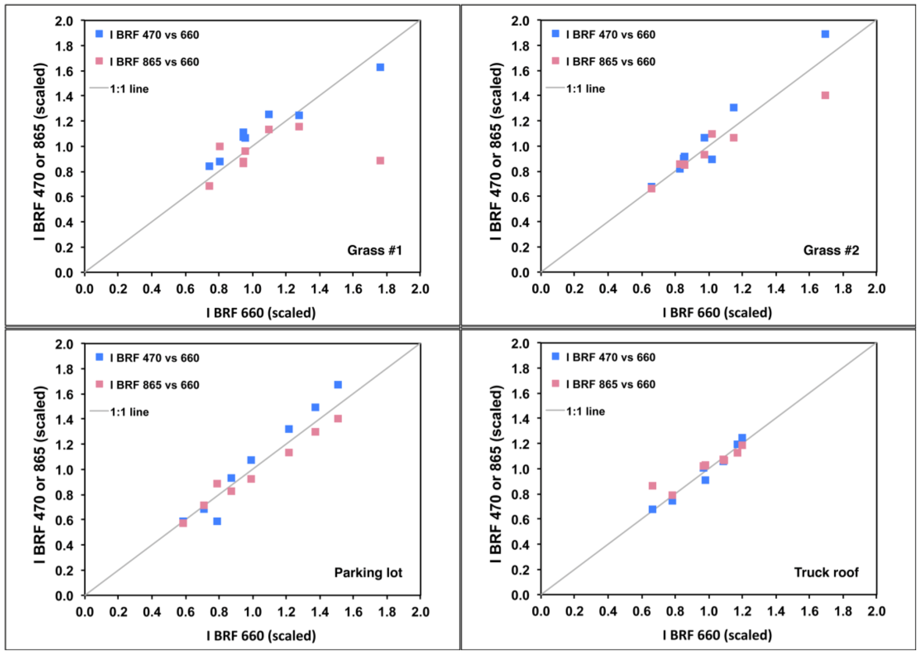
Figure 15 shows the intensity-domain BRFs (derived using Equation (23a)) at 470 and 865 nm divided by the appropriate
cλ to obtain normalized results, plotted against the corresponding values at 660 nm. Most of the data points fall very close to the 1:1 line, supporting the concept of spectral invariance of BRF angular shape. The most significant departures from this trend are at 865 nm for grass #1, and to a lesser extent for grass #2. For the grasses, the spectral BRF is significantly higher at 865 nm than in the other two bands (
cf. the
aλ values in
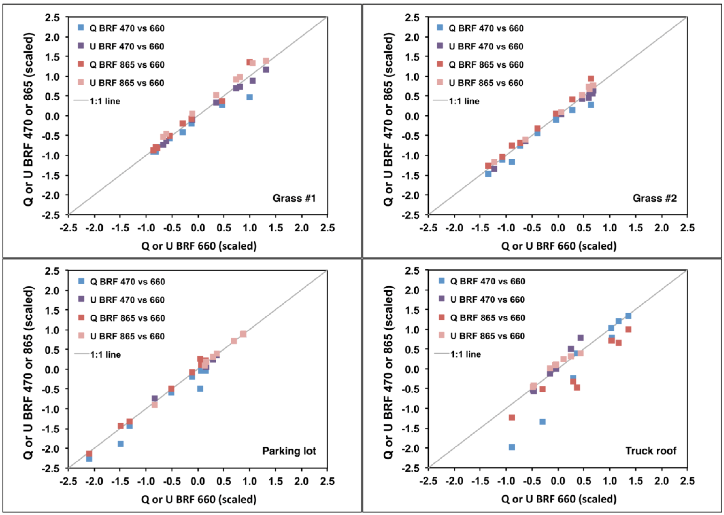
Table 1), hence the likelihood of enhanced multiple scattering and a tendency toward a more Lambertian BRF at 865 nm. For polarized BRF, the hypothesis is that the scale factor is unity, that is, both the angular shape and absolute value of polarized BRFs are spectrally invariant. This is tested in
Figure 16, which regresses scaled
BRQF and
BRUF at 470 and 865 nm against the corresponding values at 660 nm. For convenience, the scaling involved division by the wavelength-independent parameter ξ, but any wavelength-independent scale factor could be used. Because this scale factor does not depend on wavelength, adherence of the results to the 1:1 line indicates that both the magnitude as well as the angular shape of
BRQF and
BRUF are spectrally neutral. The main exception is the truck roof, which shows some departure from spectral neutrality. This may not be surprising, given that the vehicle’s paint is likely to have some variation in its complex refractive index as a function of wavelength.
Figure 15.
Intensity-domain bidirectional reflectance factors (BRFs) at 470 and 865 nm, normalized by the spectral cλvalues, plotted against corresponding values at 660 nm. The various points correspond to data acquired at different times of day. The majority of points fall on the 1:1 line, indicating that the angular shape of the BRFs are spectrally neutral, with the exception of a few 865-nm values over the grass targets.
Figure 16.
Polarization-domain BRFs at 470 and 865 nm, normalized by the spectrally invariant ξ scale factor, plotted against corresponding values at 660 nm. The various points correspond to data acquired at different times of day. The majority of points fall on the 1:1 line, indicating that both the magnitude and angular shape of the BRFs are spectrally neutral. The largest departures are observed for the truck roof.
6. Conclusions
Intensity and polarization measurements of targets imaged by the GroundMSPI spectropolarimetric camera have been compared to a surface PBRDF model. The conclusions of this comparison are as follows:
While the analytic Fresnel microfacet model commonly used to fit polarized surface bidirectional reflectance data may be sufficient to represent the reflection of diffuse skylight, it is potentially inadequate for modeling the reflection of direct sunlight because:
(a) The parameterized model leads to smooth variations of signal with angle, whereas real surfaces can show more structure;
(b) Manmade targets often have organized geometric orientations, and do not necessarily conform well to models based on random distributions of microfacets. For natural targets (e.g., soils and vegetation), the assumption of random, azimuthally isotropic facet orientations may be more appropriate;
(c) Single reflections from Fresnel surfaces over-constrain the relationship between Q and U, even if the model does a good job of fitting Ipol.
The approach, proposed in other studies, of decomposing the surface unpolarized and polarized bidirectional reflectance factors into the product of a spectrally varying function and a spectrally invariant angular shape, is supported by the GroundMSPI measurements presented here, and highlights the importance of multiangular observations to constrain aerosol retrievals. As noted by others, the polarized BRFs are more spectrally neutral than the BRFs derived from intensity data; however, the spectral invariance of the BRF angular shapes is supported by the data in both the intensity and polarization domains. For targets with significant spectral contrast (e.g., vegetation), refinement of this assumption may be warranted.
We have developed a methodology that can be applied to GroundMSPI scenes or polarization data collected by other instruments; however, many more scenes need to be analyzed to generalize the results. A much larger database of GroundMSPI imagery has been collected at JPL and at the University of Arizona, and is currently undergoing analysis to determine how well these conclusions apply to the larger data sample.
We have suggested that the geometric organization characteristic of manmade targets contributes to the lack of agreement between the single-bounce Fresnel microfacet model and the GroundMSPI polarization observations. We note, however, that the oblique view angles characteristic of these measurements, as well as their high spatial resolution, are not representative of typical remote sensing observations. Future work will examine the effects of degrading spatial resolution within GroundMSPI scenes, and will also make use of data from the airborne version of the instrument, AirMSPI, which flies on NASA’s high-altitude ER-2 aircraft. Typical footprint size of AirMSPI is ~10 m. AirMSPI view angles range between ±67° from nadir, hence are less oblique than some of the GroundMSPI views. The airborne data will enable exploring the methodology developed here in a more representative remote sensing context in which the signals from diverse surface elements are averaged over the larger sensor footprint. Should the coarser spatial resolution make it possible to use the simple, single-bounce Fresnel model for a wide variety of surface types, i.e., urban as well as natural landscapes, the results would simplify the development of a generalized satellite aerosol retrieval algorithm. On the other hand, should relaxation of the Fresnel assumption prove necessary even at coarser resolution, a potentially fruitful area of study will be the use of GroundMSPI to improve the physical basis of the surface reflection model. Establishing a quantitatively predictive mechanism whereby the P31 term of the facet Mueller matrix takes on nonzero values, e.g., multiple reflections between facets or microscale roughness anisotropy, could lead to more generally applicable surface PBRDF parameterizations that would provide valuable constraints on aerosol retrievals over land.


 . According to the law of reflection, the facet normal vector lies in the plane defined by the Sun position vector and the view vector. It is convenient to transform from a facet orientation probability density in zx, zy space to polar coordinates β, ψ because the analytic probability density functions we will use are azimuth (ψ) independent. In this case zx = tanβcosψ and zy = tanβsinψ. We note that when integrating over all possible facet orientations, the probability distributions are normalized such that:


