Technical Note

The Weather Generator Used in the Empirical Statistical Downscaling Method, WETTREG

Climate & Environment Consulting Potsdam GmbH, David-Gilly-Straße 1, D-14469 Potsdam, Germany
*
Author to whom correspondence should be addressed.
Atmosphere 2013, 4(2), 169-197; https://doi.org/10.3390/atmos4020169
Submission received: 21 December 2012 / Revised: 20 March 2013 / Accepted: 27 May 2013 / Published: 7 June 2013

Abstract

:
In this paper, the weather generator (WG) used by the empirical statistical downscaling method WETTREG (weather situation-based regionalization method (in German: WETTerlagen-basierte REGionalisierungsmethode)), is described. It belongs to the class of multi-site parametric models that aim at the representation of the spatial dependence among weather variables with conditioning on exogenous atmospheric predictors. The development of the WETTREG WG was motivated by (i) the requirement of climate impact modelers to obtain input data sets that are consistent and can be produced in a relatively economic way and (ii) the well-sustained hypothesis that large scale atmospheric features are well reproduced by climate models and can be used as a link to regional climate. The WG operates at daily temporal resolution. The conditioning factor is the temporal development of the frequency distribution of circulation patterns. Following a brief description of the strategy of classifying circulation patterns that have a strong link to regional climate, the bulk of this paper is devoted to a description of the WG itself. This includes aspects, such as the utilized building blocks, seasonality or the methodology with which a signature of climate change is imprinted onto the generated time series. Further attention is given to particularities of the WG’s conditioning processes, as well as to extremes, areal representativity and the interface of WGs and user requirements.

1. Introduction

Weather generators (WG) are parametric stochastic models (i.e., mathematical formulations that explicitly include elements of randomness) emulating weather data [1]. In other words, they are algorithms that are devised with the intention to synthesize time series that are conditioned by external factors—of (in principle) unlimited length and number. The emulation encompasses the capability to generate daily weather that is statistically similar to the observed weather [2]. This approach is necessary, e.g., to add climatic signatures to these series, particularly the signatures of a changing climate.
The need to use synthesized, yet realistic, weather, preferably in daily resolution, as an input for models, e.g., in the domains of climate impact research, environment, ecology or hydrology, led to the development of problem-specific WGs in the 1980s and 1990s (e.g., [3,4,5]). The Core Project BAHC (Biospheric Aspects of the Hydrological Cycle) of the IGBP (International Geosphere Biosphere Programme [6]) aimed at, among other tasks, a harmonization of the independently developed WG approaches, as documented in [7].
Stochastic procedures are frequently applied (as described in [8]) when the object of study, e.g., precipitation, is not well represented in atmospheric models on a small scale, on the one hand, but these models, on the other hand, exhibit skill with respect to long-lived large scale atmospheric circulation patterns [9]. The approaches can incorporate Markov chains, as, e.g., in [10,11] or [12], or make use of WGs, as, e.g., in [13] or [14], which additionally focuses on the description of future climates. Linking circulation patterns with weather-generating algorithms has been carried out in studies of regional climate impact, e.g., by [15], for Germany using the empirical Großweather situations of Hess/Brezowski (described in [16] ) or by [17] for Portugal using objectively derived circulation patterns. The background and the development of “weather generating” methods are well covered in two review articles [1,18].
As an alternative approach, the method of [19] constitutes a multi-station, multi-element WG, which provides a climate scenario regionalization. It is conditioned by temperature trend developments; the results for other climate parameters are determined according to their dependency on the temperature development.
Hayhoe [20] extended the WG principle to synthesize the time series of precipitation, as well as solar radiation, maximum and minimum temperature. Station-wise comparisons of measured and generated time series for locations in Canada yielded highly significant similarities, also with respect to derived properties of the generated series, such as the length-distribution of frost-free periods and of wet periods.
It is rather demanding to expect that a WG is able to synthesize time series that exhibit similarity to the observed daily weather with respect to mean values and variability. [21] broadened the scope and included the representation of extremes. According to this study, a mismatch of the mean and extreme value distributions is an important reason for systematic biases in the extremes, particularly concerning temperature. More recent developments with respect to multi-site modelling propose the construction of so-called copulas, as described, e.g., in [22].
In the following sections of the paper, a WG is featured that forms the core of the empirical statistical downscaling (ESD) method, WETTREG (weather situation-based regionalization method–in German: WETTerlagen-basierte REGionalisierungsmethode) (cf. [23,24]). The method’s development dates back to projects in the mid-1990s [25] and is in a process of continuous refinement [26,27]. The weather generator component was further developed and is described, e.g., in [28,29]. Some WG-specific background is covered in [27]. It belongs to the class of multi-site parametric models, which, in addition, aim at the representation of the spatial dependence among weather variables with conditioning on exogenous atmospheric predictors [30] operating at daily temporal resolution.
The essential steps of the WETTREG WG are sketched in Figure 1. Basically, it assembles segments of existing data (time series of atmospheric measurements in daily resolution, denoted by magenta boxes A, B and C in Figure 1 in a stochastic way to form alternative versions of weather processes. The assembly procedure (green box, denoted D) is governed by (i) the frequency distribution of large scale circulation patterns (blue boxes, denoted F and G, in Figure 1 and (ii) a set of criteria (red box, denoted H, in Figure 1) that control the selection or rejection of candidate segments in order to imprint a climate change signal onto the time series.
Figure 1. Flowchart of the WETTREG weather generator (WG). The various aspects are described in the sections of this paper.
Atmosphere 04 00169 g001
Since the WG is a component of an ESD method, a further transfer step (signified by box E in Figure 1) takes place. It encompasses a fanning out of the aggregated, i.e., areally averaged information, that emerged from the pre-processing towards the locations of the network of stations used.
It should be noted that this seemingly straightforward procedure is riddled with sensitivities, e.g., with respect to the set of selection/rejection criteria that govern the WG. Users of WG-produced local time series should be aware of the advantages, but also, the shortcomings of the synthesized time series in order to realistically assess what can be achieved with these series [31].
The paper is structured as follows: Prerequisites and background concerning the circulation pattern concept are provided in Section 2. The description of the methodology and a discussion of specific features of the WG can be found in Section 3. The transition from areally averaged (i.e., by computing the mean value of a variable from a set of stations in the target area) to local time series is dealt with in Section 4. Remarks on the comparability of downscaling methods that employ WGs are given in Section 5. Remarks on core aspects of the WETTREG WG are presented in Section 6, followed by a summary and outlook in Section 7.

2. Before the WG is Launched

The reader might expect a “Data and Method” section at this stage. However, this is a “Method” paper, and therefore, the prerequisites of the WG are summarized in this section, including the required data and an explanation of what we mean by “patterns”.

2.1. Data

As indicated by the orange and light blue boxes in the top portion of Figure 1, applying WETTREG and its WG requires several types of data:
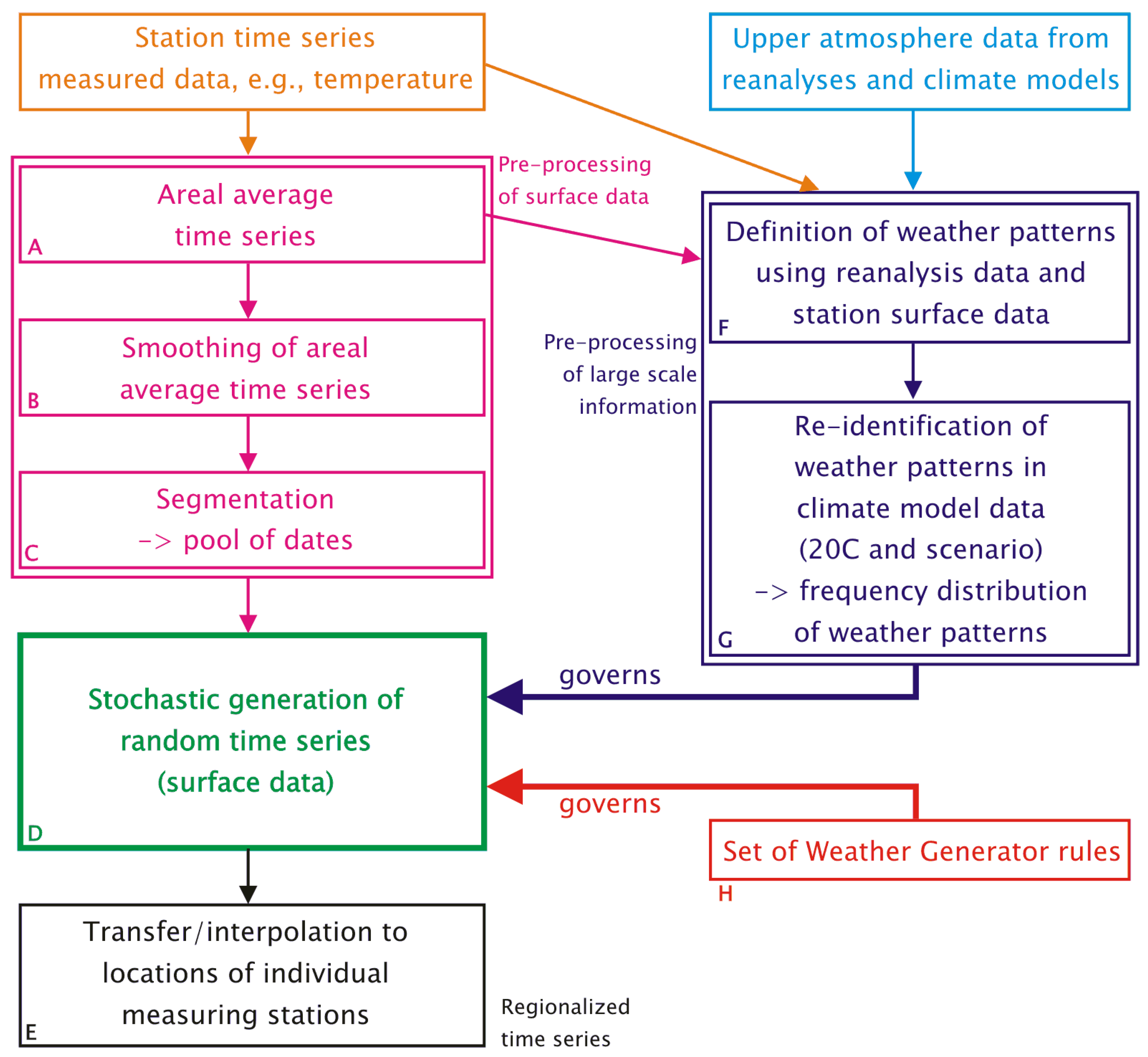
  • Surface observations from the region of interest. This encompasses a number of weather elements (e.g., daily values of temperature, precipitation, sunshine duration, cloudiness, humidity, air pressure, wind) measured at climate stations or precipitation stations. In the course of the pre-processing towards the usage in the WG (boxes A, B and C in Figure 1), surface data are aggregated into regional averages, which are subsequently segmented into episodes. Moreover, the particular method by which WETTREG defines its circulation patterns (see Section 2.2 and Section 3.3), requires aggregated surface observation data, too.
  • Atmosphere data based on measurements and homogenized by reanalysis form a kind of three-dimensional climatology of the recent past. Several reanalysis products were developed and are in frequent use: NCEP (National Center for Environmental Prediction) [32], ERA40 [33] and, most recently, ERA-Interim [34]. The philosophy and strategies of reanalysis are described, e.g., in [35] and [36]. In order to cover a period from the 1970s to the early 21st century, NCEP reanalyses are used in the pattern-development stage of WETTREG (cf. box F in Figure 1 and Section 3.3).
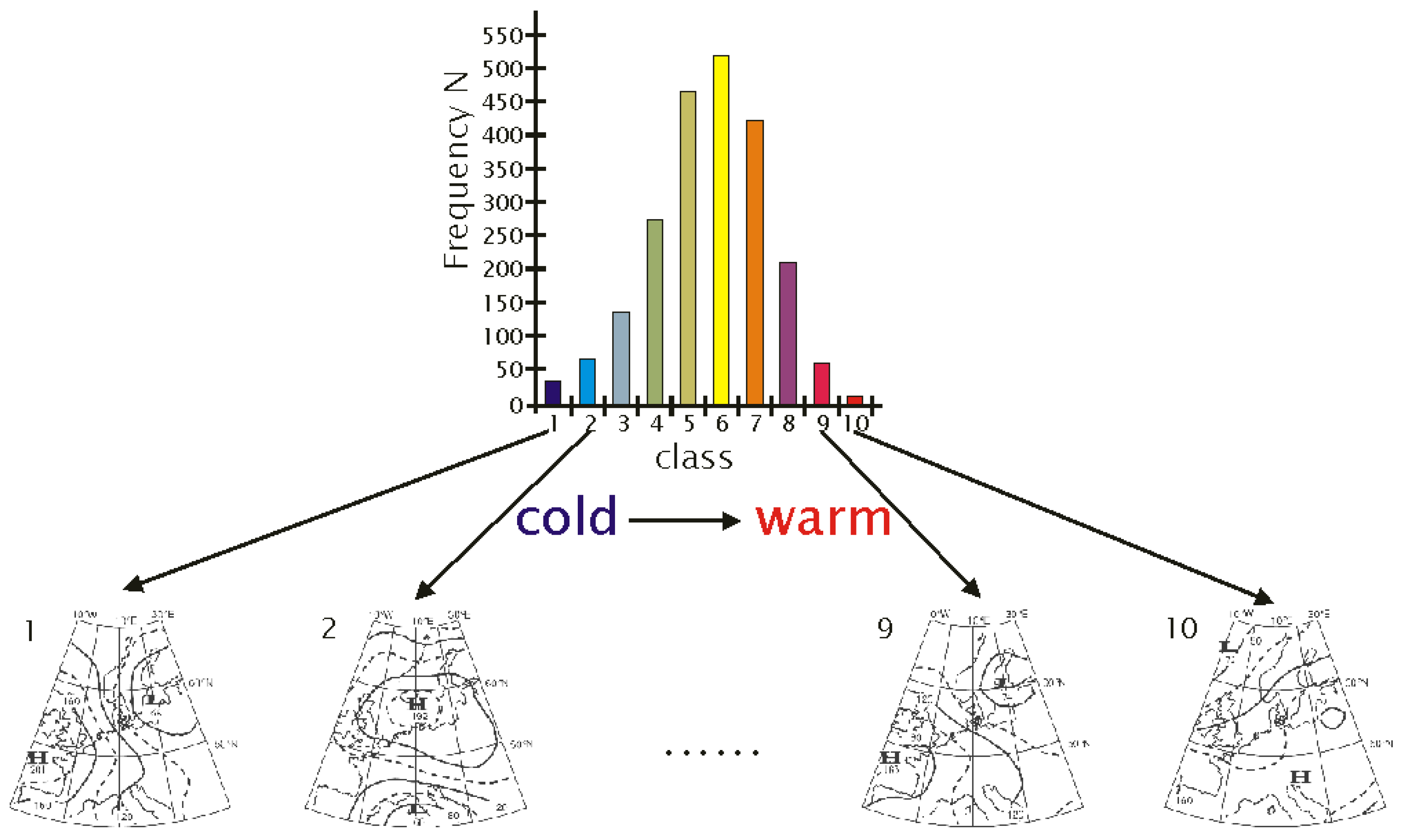
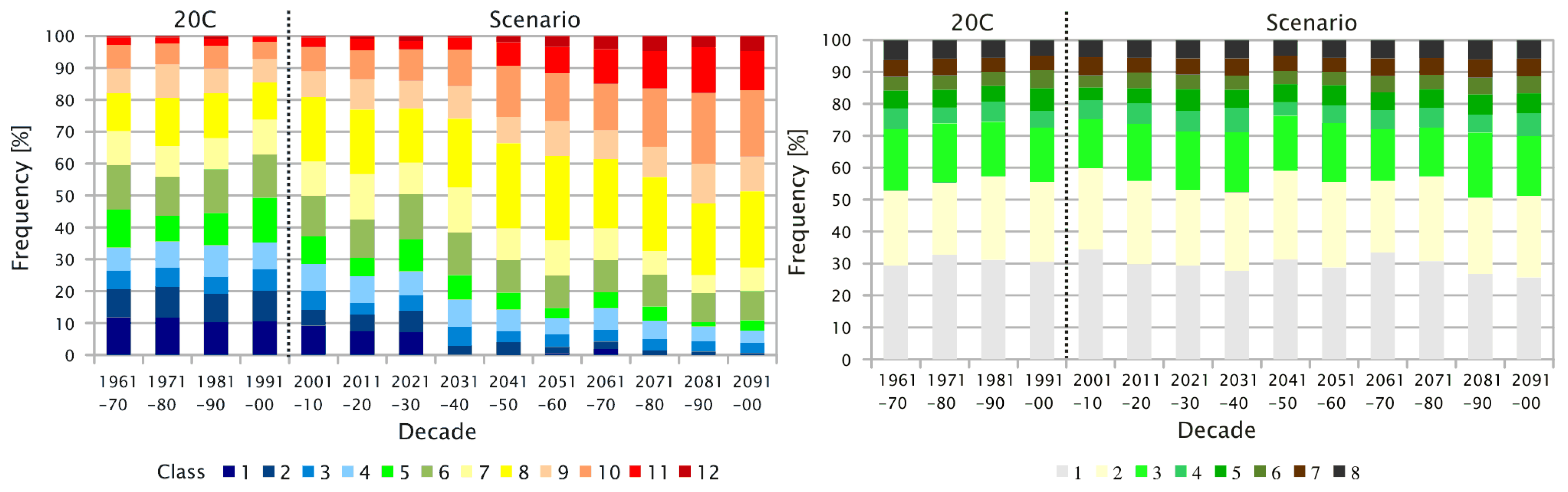
  • Atmosphere data for the European region from a Global Circulation Model (GCM). Recently, also, Regional Climate Models (RCMs) have been run for a similarly large area, enabling WETTREG to use them as an alternative input data source [24].
    Eight upper air fields, i.e., geopotential height (at 1,000, 850, 700 and 500 hPa), temperature and humidity at 850 and 500 hPa are extracted for the description of the 12 UTC conditions, as is simulated by the circulation model. So called 20C data are used for the model’s re-simulation of the current climate, and data from the model forced by a scenario, e.g., an emission scenario GCM run, based on the Special Report on Emissions Scenarios (SRES) [37] or representative concentration pathways (RCPs) [38] type, are used for the assessment of future climate conditions. As indicated by box G of Figure 1 and described in Section 3.3, the circulation model data are analyzed with respect to the frequency of the aforementioned circulation patterns—for details, please refer to Section 2.2. The changing frequency distribution is a governing factor for the WG.

2.2. Circulation Patterns

Identifying an adequate property for the selection/rejection process that governs a WG has spawned a host of different approaches. Depending on the atmospheric property at hand (precipitation, radiation, temperature), it can be required that the synthesized time series represents the frequency of occurrence for dry or wet days (from Markov chains to other determining strategies, as, e.g., in [1,5,8,10,11,39]).
The ESD method, WETTREG, on the other hand, seeks to identify a link between large scale information and corresponding information on the regional scale. That link, or transfer function, is provided by a circulation pattern classification. According to [40], the transfer function applied in an ESD method needs to fulfil four necessary conditions: strong relationship, model representation, description of change and stationarity. However, this paper does not address these four conditions, with regard to, the WETTREG method. Details can be found in [23,26,41].
Circulation pattern classification is a methodology to organize the wealth of atmospheric features—circulation patterns—into distinct classes. What might their contribution to understanding and assessing climate change be? The rationale for applying the pattern strategy to downscaling climate model data refers to a statement of F. Giorgi in [42]: If you don’t believe in the value of global climate models, then there’s no point in downscaling them. But if you do—and global models do provide a quite consistent pattern of climate change—then it makes sense to translate global patterns into local information. The WETTREG method is an application of Giorgi’s hypothesis, i.e., the existence of a linkage between the regional and large scale. An other study, also applying a WG in a circulation pattern context, can be found in [15].
In practice, the patterns of WETTREG are not defined according to the circulation-to-environment principle (a strategy applied in synoptic climatology, described, e.g., in [43]). According to this principle, groups (classes) of atmospheric features are formed according to their morphological properties, identifying phenomenological similarities. The circulation-to-environment approach is, nevertheless, in frequent use. It is applied by subjective classifications, such as the Grosswetterlagen of Hess and Brezowsky [16], and is common to all classification approaches used in a European Cooperation in Science and Technology (COST) Action, presented in [44] and [45].
Rather, the WETTREG patterns are built “from the region up”—a principle, which in the nomenclature of [43], is called environment-to-circulation. Applying this principle means that the classification is carried out according to a climate parameter. For this purpose, WETTREG employs measurements from a network of surface stations—aggregated to areal averages (see boxes A and B in Figure 1), e.g., by putting all days within a specific surface temperature range into one class and those within the adjacent higher temperature range in an other class, and so on. Figure 2 visualizes the assignment of individual days to their respective “temperature class”, which constitutes the initial step for the circulation pattern classification that WETTREG uses. It should be added that the classification is carried out separately for the meteorological seasons (Spring⇁March-April-May (MAM); summer⇁June-July-August (JJA); autumn⇁September-October-November (SON); winter⇁December-January-February (DJF)), which incorporates the seasonality of the climate regime. As a brief look ahead, it has to be mentioned that as a consequence of this approach, seasonal breaks occur in the WG-produced time series; counter-measures will be shown in Section 3.6.
Figure 2. Sketch of the initialization of circulation pattern classes, building a frequency distribution of days belonging to different ranges of regionally aggregated temperature (upper part) and the formation of composita for each temperature range class (lower part), as carried out in WETTREG.
Atmosphere 04 00169 g002
The assignment of individual days to the classes based on the temperature values at this stage is a preliminary one. The final assignment of the days to the classes follows this scheme: (i) composita are formed by grouping upper air fields from reanalysis data (cf. Section 2.1) of all days that belong to a class, as sketched in the bottom part of Figure 2—thus, determining the morphological features common to each class; (ii) in a test pass, the upper air fields of each day are compared to all composita-generated patterns using the similarity measure, S M (Equation (1)), a root mean square distance kind of relation, which compares pairs of field values.
In [26] and [27] the background for such a procedure was presented. Suffice it to mention in the context of describing the pattern frequency-driven WG of WETTREG that several upper air fields (such as geopotential, temperature, humidity, relative topography, advection, vorticity, derived from several levels between 1,000 and 500 hPa) are being used. The selection of the fields (up to four of them) is subject to a screening regression applied to reanalysis and surface measurements for the target area, which identifies the most appropriate large-scale upper air fields applicable to describe surface climate parameters. So, Equation (1) is in fact not applied to a single field, but to a group of up to four fields determined by the screening regression. In order to perform the evaluation of the field pairs (composita and days-to-be-tested) and taking different orders of magnitude of those fields into account, they need to be normalized beforehand.
This means that it is allowed that morphological similarity overrules the initial class assignment by temperature value, yielding the optimally matching pattern. However, the majority of the days remain in the class initially assigned by the temperature range—if changes occur, they are predominantly for the adjacent classes.
S M k = i , j = 0 i = m , j = n C o m p ( i , j ) k T D ( i , j ) 2
with S M : similarity measure; k: ordinal number of the compositum pattern for which the testing is performed; i , j : co-ordinates of the two fields; m , n : number of the grid points along the i- and j-axes, respectively; C o m p k : k th field generated in the composita-building process, as sketched in the bottom part of Figure 2; and TD: day to be tested for similarity, i.e., individual day for which the assignment to the optimal match is to be determined. S M k m i n determines the assignment to the most similar class, k.
The result of the environment-to-circulation-derived procedure is a set of classes and their morphological properties. These represent well separated mean large-scale circulation patterns that can be supposed as “causing” certain temperature range classes. For completeness’ sake it should be added that a classification according to value ranges of (regionally averaged) rainfall amounts is carried out, as well, yielding precipitation patterns.
With the set of (season-specific) circulation patterns in place, the analysis is continued using daily realizations of a climate model. The strategy of testing for morphological similarity is applied again, this time, evaluating Equation (1) with pairs of field values from the composita described above and individual modelled days in 20C or scenario runs of a climate model. This assignment of the model data to their most suitable large-scale pattern is a process also called “re-identification” in this paper.
Performing the re-identification for all days yields frequency distributions of cold…warm patterns (or dry…wet patterns, if precipitation is considered) and their development over time according to climate model re-simulations of the current conditions (20C data), and the projected future climate (scenario data), as indicated in box G of Figure 1 and exemplified in Figure 3. For more details, see [41] and [23]. The latter reference, in Section 2.1, also addresses the problem of “optimum complexity”, i.e., determining an appropriate number of classes. Related considerations and extended empirical testing led to the usage of 12 temperature classes and eight precipitation classes in WETTREG.
Figure 3 gives an example for changing circulation pattern frequencies, aggregated decadally (here, frequencies of classes defined according to the regional winter temperature and precipitation conditions in Saxony). Clearly, in the early decades of the 21st century, up to about 2030, the distributions of the temperature patterns (left panel of Figure 3) assume a shape resembling that of a normal distribution, which means that relatively high frequencies occur for the center classes 4–9, and a tapering-off towards the lowest (coldest) and the highest (warmest) classes can be traced. Over the course of the century, the shape of this distribution changes somewhat: the “cold” classes are gradually decreasing in frequency, and for the last decades of the 21st century, on the order of 50% or more of all days are projected to be in the “warmest” classes, i.e., #9 and higher.
Figure 3. Example for the temporal development of the frequencies of 12 WETTREG temperature patterns (left) and eight precipitation patterns (right), as they are re-identified in a model run by ECHAM5/MPI-OM T63L31 run 1 [46,47]. 1961–2000: ECHAM5 forced by 20C data. 2001–2100: ECHAM5 forced by SRES scenario A1B data. Region: Saxony. Season: winter.
Atmosphere 04 00169 g003
With respect to the frequency distribution of the precipitation patterns (right panel of Figure 3), the “dry” class (pattern #1) is most frequent, accounting for about 30% of all days. There is little development of the precipitation classes’ frequency distribution over time.
This section dealt with the prerequisites for one of the factors that governs the operation of the WG, given in the upper right hand portion of Figure 1: the dependency on the temporal development of the circulation regime. It focused on these two aspects: (i) establishing the environment-to-circulation concept and its implementation in WETTREG; and (ii) deriving the changing frequency of those circulation patterns. The following section will address the generation of “building material” used by the WG, as well as the methodology of the WG itself.

3. Description of the Weather Generator

The WG in WETTREG is (i) stochastic and (ii) produces material for synthesizing time series in which there is a link between regional climate and large-scale atmospheric features (Figure 4). Essentially, a time series is assembled using building blocks from the current climate, guided by an algorithm. The WG itself first constructs the building blocks from observed time series. It then prescribes the sequencing, i.e., the information, from which particular strings of days from the observed climate are to be selected (Figure 5).
Figure 4. Schematic of the pre-processing steps that lead to the data base used by the WG to synthesize time series. Temperature time series from a target area are averaged, smoothed and segmented to form a pool of dates. The individual steps are described in the text.
Atmosphere 04 00169 g004
Figure 5. Schematic of the selection process. The segmentation process (Figure 4) leads to the pool of dates. The WG selects some of them according to criteria described in Section 3. Episodes are assembled to form time series (cf. Figure 9).
Atmosphere 04 00169 g005
In order to arrive at a pool of building blocks, a few pre-processing steps are necessary—those appear as boxes A, B and C in the top left portion of Figure 1. A schematic of these steps is depicted in Figure 4.
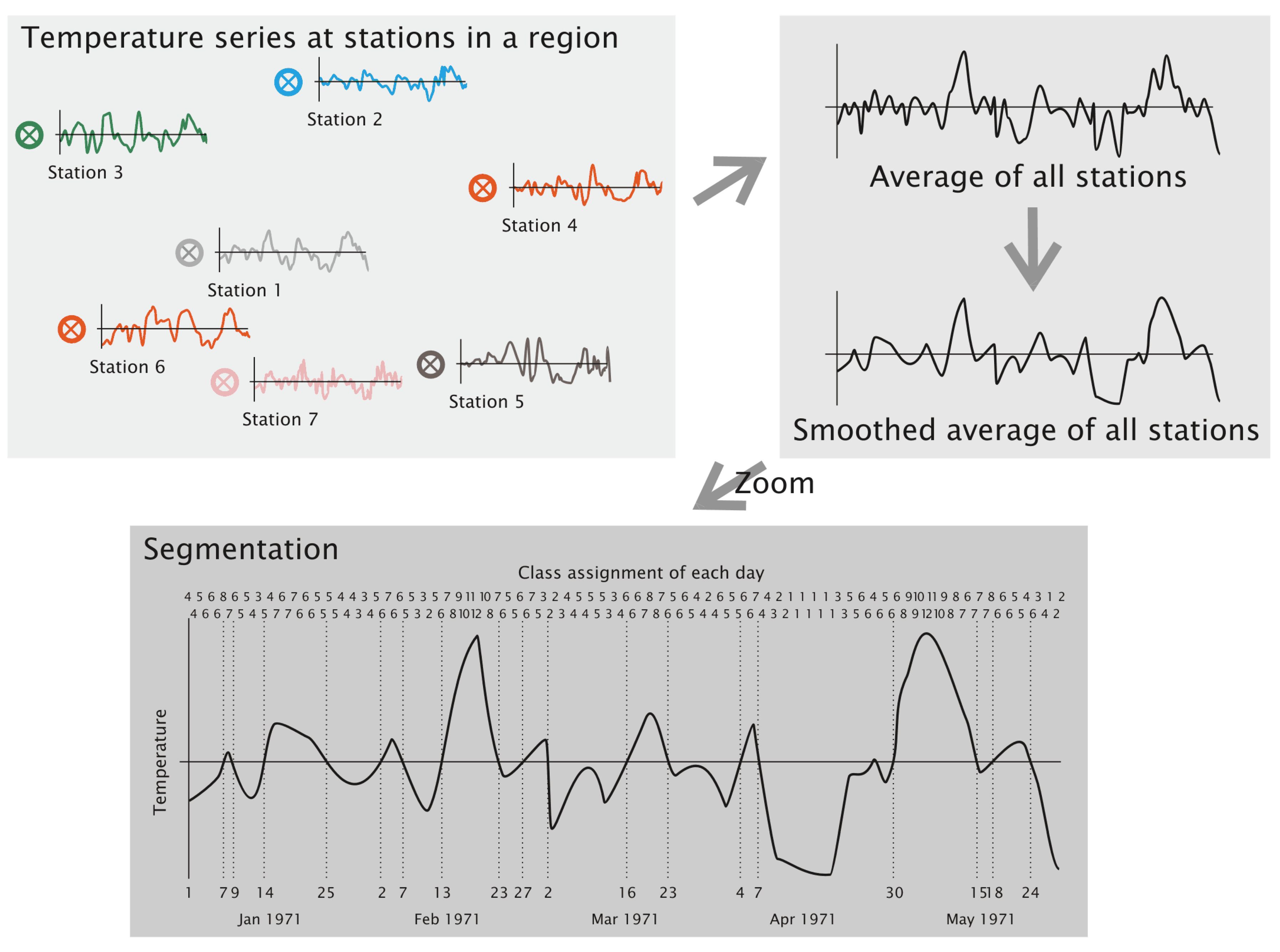
  • A target area is selected, and time series of surface climate parameters are identified. However, only the temperature is used for the subsequent pre-processing steps. It is the aim of the authors to keep the method description as simple and straightforward as possible. Therefore, the examples are build up using temperature time series. In the method’s implementation, time series of deviation from the annual temperature cycle are used, which is, however, of little relevance for understanding the method’s principles.
  • Areal averages—the arithmetic means of all stations from the target area—of the temperature are computed for each day.
  • A five-point smoothing using equal weights is applied (example: the temperature on January 10 is replaced by the average temperature of January 8 to 12). Beginnings and endings of the time series use the average computed from three or four days, respectively.
  • The smoothed time series is cut into segments whenever a pass through zero occurs.
One feature of the bottom panel of Figure 4 should be highlighted, because it is instrumental for the understanding of the WETTREG WG principle: the row of numbers above the curve, which, for readability’s sake, are displayed in shifted form. It includes the assigned circulation patterns that were introduced in Section 2.2. Therefore, each segment also carries a frequency distribution of those patterns, which is one of the features in Figure 6.
The WG itself (represented by box D in Figure 1, the principle is depicted in Figure 5) then synthesizes time series by randomly drawing episodes from the segmented pool. In fact, the WG itself follows the principle of indirect addressing, known from software development. The bins of the episode pool contains the beginning dates and the lengths of the episodes, which then are used to track the respective temperature episodes to be tested for insertion into the emerging synthesized time series. Thus, it is rather a pool of dates. Whether an episode is accepted as a building block or rejected is subject to a set of governing criteria.
The list below highlights aspects, boundary conditions, interdependencies and noteworthy considerations, which address (i) a rationale for aggregating temperature times series into regional averages; or (ii) details in the process of segmentation; or (iii) optimization strategies for the set of acceptance/rejection criteria of the WG. Attention is given to the fact that the synthesized series need to be similar, but not identical. Thus, there is the need for a carefully designed “dose of randomness” in the selection process (for a further elaboration of this aspect see Section 3.4). Another important factor is the inclusion of seasonality, bearing in mind that the annual cycle needs to be featured in the synthesized time series smoothly, as well as in a representative way; for related details, see Section 3.6.
The labels of the list items below correspond to the second digit of the subsection numbers of this section in which the highlighted aspects are expanded and discussed.
  • Usage of an areal average to generate the pool of dates instead of a station-wise series synthesizing procedure (Section 3.1);
  • assembly of episodes of g and h days-length (Section 3.2);
  • frequency of circulation patterns as the main governing factor for optimizing the time series synthesized by the WG (Section 3.3);
  • measures to ensure the stochasticity of the the synthesizing process (Section 3.4);
  • approximation of synoptical and statistical climate properties (Section 3.5);
  • overlapping frequency distribution as a measure of dealing with seasonality (Section 3.6).
Figure 6. Illustration of the building blocks and the prescribed frequency distributions that govern the selection/rejection criteria of the WG. The yellow-shaded part shows two sample episodes. The temperature axes indicate that the episode depicted left contains warm days (temperature average over the target area) and that the right episode contains cold days. Also shown is the assignment to the temperature-dependent circulation patters (cf. Section 2.2). The rows of numbers underneath the curves denote the numbers of the patterns assigned to the respective days of the episodes, as well as frequency distributions for patterns 1...12 in both episodes. The bottom panel (gray shading) sketches the target distributions at the beginning (left) and the end (right) of the 21st century. They are needed in the synthesizing process described in the flow schematic in Section 3.3.
Atmosphere 04 00169 g006

3.1. Why Areal Averaging?

It is assumed that a set of measuring stations exists in the target region. As shown in Figure 2 and Figure 4, the stations’ time series are aggregated to form (i) the basis for the circulation pattern classification (see Section 2.2) and (ii) a regional temperature average, segmented for the pool of dates and including the assigned classification patterns for each day.
Since the described WG is employed as part of a downscaling method, straying away from the principle of areal aggregation would have repercussions to the stage in which the local climate information is generated from the synthesized series of areal averages (cf. Section 4). If the WG would synthesize the series of individual stations, it would be highly probable that these series were “out of synch”. This means that, due to the station-specific pattern classification and synthesizing process, different sequences of episodes, including different days, would be used in the series for the individual stations. Consequently, there would be inconsistencies (i) when applying the information prescribed by the WG to the series at individual stations and (ii) when assessing the behaviour of a meteorological variable in the space between the stations. The solution is therefore to compute an areal average of the physical property that the WG is using, i.e., the temperature.

3.2. Episodes and Their Length

Generally speaking, the rationale for using episodes and not individual days as building blocks in the WG is that the atmosphere system can be hypothesized as a kind of “analogue computer”. On a meta level, the weather processes that are sampled in an episode are interconnected. Physical and chemical processes in the earth’s climate system “take care” of a truthful linkage, e.g., between cloudiness, temperature and humidity. Thus, the interruptions in this “natural flow” should be as seldom as possible.
When a time series is synthesized, episodes of weather that indeed occurred are used, as sketched in Figure 4. In the example, the episodes are beginning and ending at a zero-crossing of the regional averaged temperature, i.e., for temperature, an episode is a sequence of days above or below some defined threshold. The episodes themselves are from a defined time interval, e.g., 1971–2010. It is of advantage to use a rather long time interval for building the pool, not necessarily congruent with WMO-endorsed climate normal periods [48]. One reason is to give the pool a greater diversity to draw from. A second reason is related to a fact that emerges from the aim of reproducing a changing, more extreme, climate: meeting these demands benefits from the existence of building blocks, which include episodes that contain rather extreme values of the meteorological parameters; the frequency of these occurrences has been going up in the recent past.
The description of the segmentation visualized in Figure 4 focused on the usage of zero-crossings of the temperature as episode delimiters. This is adequate when applying the WG to reproduce current climate conditions. If a future, warmer climate is to be to reproduced, this leads to problems. Broadly speaking, when the WG synthesizes a time series for such a changed climate. there are fewer “cold” episodes requested. This effect is reduced when other definitions for the beginning and end of an episode are employed, as well. Therefore, the pool is complemented by sequences of days that are all above a certain temperature threshold, i.e., not cut at zero crossings.
It should be added that, although all segments are available to the WG as candidates, it is restricted to use only those which have a minimum length g of seven days and a maximum length h of 60 days.
Remark 1: When synthesizing the new time series, the linkage between temperature and precipitation is acknowledged by using both frequency distributions (temperature and precipitation) as the target for a fitting process, described in Section 3.3, with a weight of 0.8 for the temperature classes and 0.2 for the precipitation classes. In order to describe the WG’s principles and for the sake of a better method understandability, the examples show distributions of the temperature classes only. Occasionally, reference is made to the fact that there are actually two distributions that govern the goodness-of-fit measure for the synthesizing of temperature series. The matter is becoming even more complicated, because the synthesizing of time series according to precipitation criteria uses the frequency distributions of precipitation classes alone; the reader is kindly asked to bear with this slightly simplified description.
Remark 2: The contents of the pool of dates points to pieces of the segmented temperature time series, exclusively—there is no pool that would be linked to “precipitation episodes”.

3.3. The Synthesizing Process Controlled by Pattern Distributions

Incorporating changes of large-scale atmospheric properties as governing factors into a WG constitutes a novelty, particularly in conjunction with patterns that are derived in an environment-to-circulation way (cf. Section 2.2 and Figure 2). A few basic facts need to be kept in mind:
  • No matter if the individual days are from reanalysis data, 20C simulations or climate model scenario runs, each day had been assigned to a circulation pattern (cf. Section 2.2) during the patterns-matching phase (cf. Equation (1)).
    -
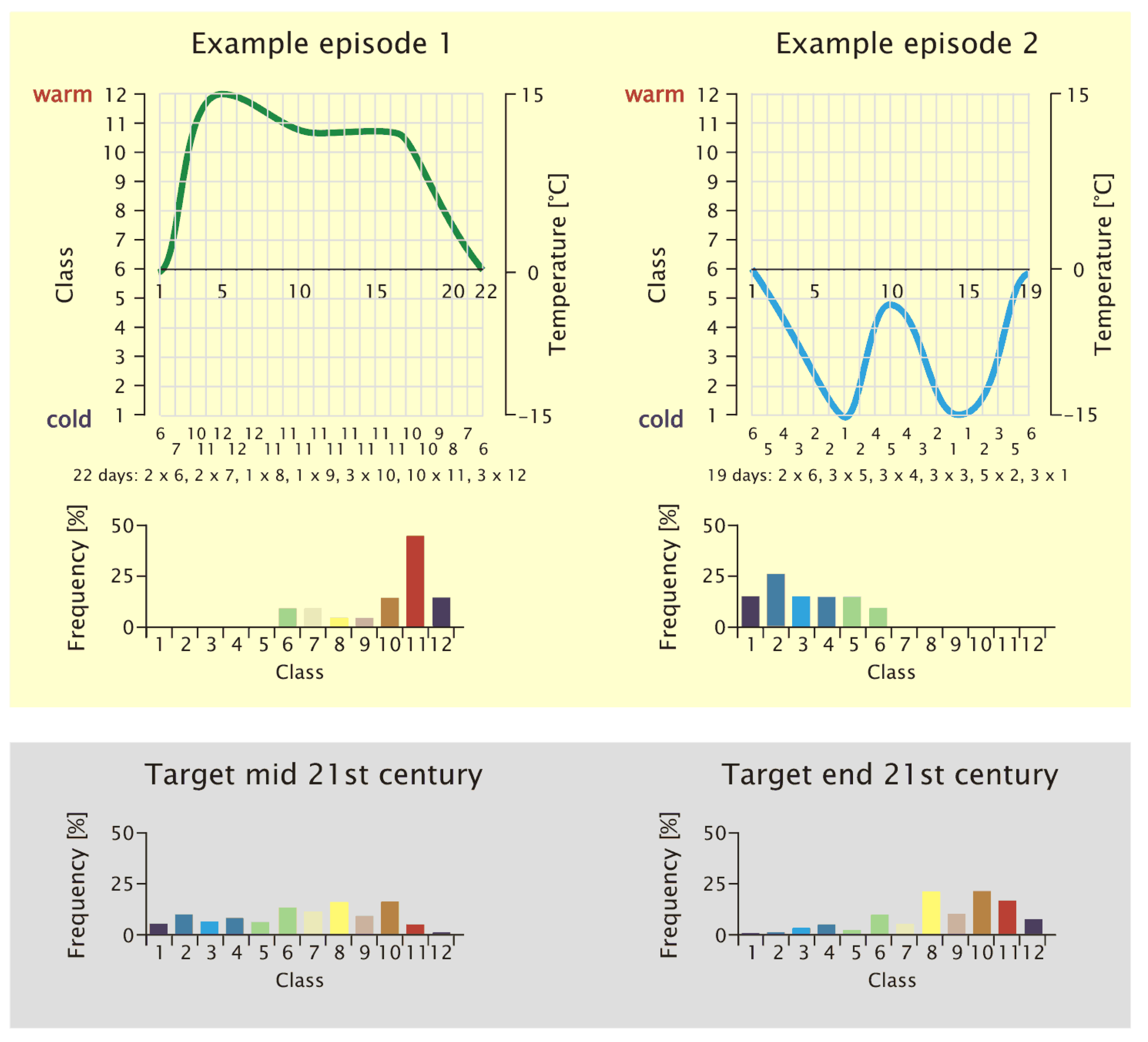
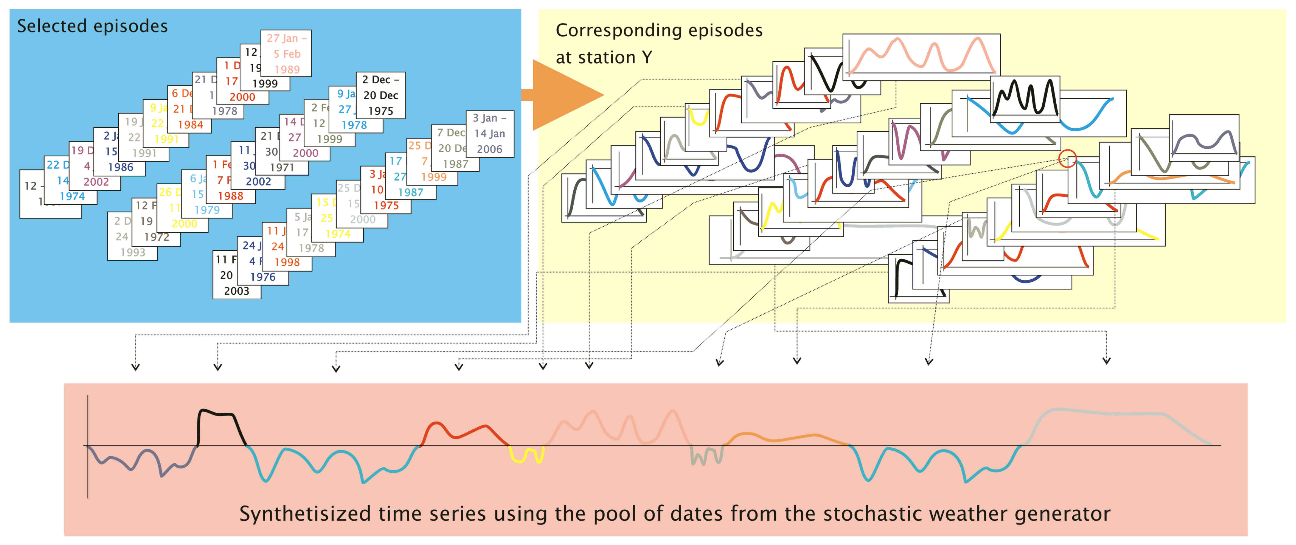
    The sequence of days that belongs to an episode (determined from the current climate conditions as they were measured) carries a frequency distribution of these patterns, as shown in Figure 6. Since the WG strings together episodes that actually occurred, to form new time series, these episodes constitute the building blocks of the emerging time series. Their inherent pattern frequency distribution is evaluated.
    -
    Concerning the days of the 20C runs from a climate model, the determined frequency distribution of circulation patterns constitute the model’s ability to reproduce what was established by way of analyzing reanalysis data and surface measurements.
    -
    Concerning the days of the scenario runs from a climate model, the determined frequency distribution of circulation patterns constitute the model’s projection of a future climate, adhering to the circulation patterns established by way of analyzing reanalysis data and surface measurements.
  • The underlying (or target) frequency distribution of the circulation patterns determined from a circulation model is determined (20C or scenario run, depending on the time frame of interest). An example is given in Figure 3.
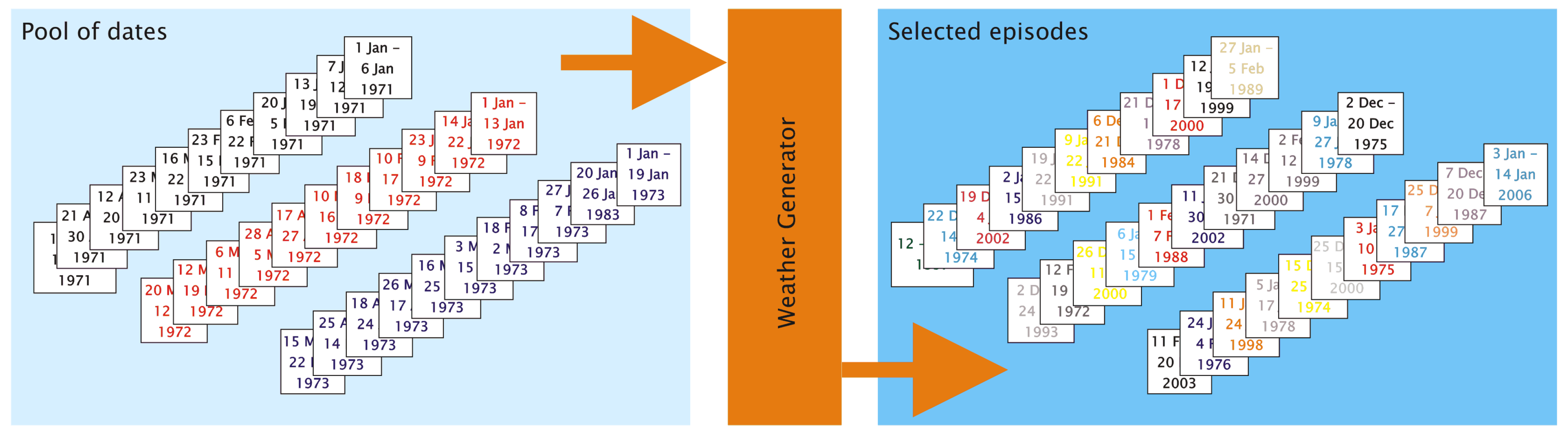
  • The synthesizing process successively generates a string of episodes and is represented by the loop below. The members of the episodes pool are tested one by one if they help optimize the goodness-of-fit between the pattern frequency distribution of the synthesized time series, on the one hand, and the target frequency distribution, on the other hand. One “optimal” episode is determined per pass.
Within the WG of WETTREG, the following steps are taken and summarized in the flow schematic below. Beforehand, the time frame of the series is prescribed, e.g., the entire span from 1 January 1951, to 31 December 2100, might be synthesized. The counter, N, of the series-to-be-synthesized is initialized with a value of one and the track is kept on the initial date for the synthesized time series.
  • Selection process for adding the Nth episode to the synthesized time series is launched.
  • Episode E s from the pool of p dates is selected. This is the “candidate episode”.
    • If it is the very first episode ( N = 1 ) in the synthesizing procedure, the subsequent evaluation steps are carried out using the frequency distribution, F r e q t e s t of E i (cf. Equation (2)) this candidate episode alone vs. the underlying (target) frequency distribution.
    • If a successful candidate has been assigned to the emerging synthesized time series ( N > 1 ), a pooled frequency distribution of all members, accepted so far into the series, emerges, as well. Each new “candidate episode”, E i , is provisionally added to that pooled distribution, and the evaluation steps are then carried out with the provisionally generated frequency distribution until an optimal candidate has been determined.
  • The goodness-of-fit measure, G F (see Equation (2)), is used to determine the degree of match between the pattern frequency distribution within the synthesized time series (including the candidate episode) and that of the circulation model data for a certain time horizon (the prescribed target frequency distribution, shown in the gray shaded area of Figure 6).
  • It is evaluated if adding that episode to the time series synthesized so far improves or deteriorates the fit to the prescribed target frequency distributions, by determining if G F for this pass. Track is kept on the pass number s and its G F measure.
  • If the counter, s, is below or equal to the number of episodes in the pool of dates, i.e., p, then s is increased by one. The loop is repeated, starting at entry number 2 above. It should be noted that at each pass, the entire pool of dates is evaluated, i.e., the same episode can be selected repeatedly.
  • When all p episodes have been tested, the candidate episode, E o , that yielded the minimum of all G F values for the s passes is added to the emerging synthesized time series.
  • Track is kept on the origin of the episode (i.e., day, month and year of its beginning, as well as its length, all extracted from the pool of dates), the date in the synthesized series for which the inserted episode is being used and information pertaining to the newly added episode (such as measured meteorological parameters or assigned circulation pattern).
  • As long as the final day, initially specified for the synthesized time series, has not been reached, the counter, N, is increased by one. The loop process is repeated starting at entry number 1, above.
The principle of the day-to-class assignment is sketched in Figure 6 for two sample episodes containing warm and cold days, respectively. Moreover, the count of the classes in these episodes and their frequency distribution is given below the graphs in the yellow-shaded part of the figure. The gray-shaded bottom part of Figure 6 signifies the shifting frequency distribution of the classes over time, i.e., the target frequency distribution.
As mentioned in several entries of the flow schematic above, a test statistic is required to determine if an added candidate episode into the emerging synthesized time series improves or aggravates the goodness-of-fit with respect to a prescribed (or target) frequency distribution. This G F measure, basically a relation of the root-mean-square-distance type, is shown in Equation (2).
G F = i = 1 n F r e q ( i ) p o o l F r e q ( i ) t a r g e t 2
with G F : goodness-of-fit measure; i: enumerator for the different bins of a frequency distribution (exemplified by the 12 temperature classes depicted in the frequency distributions in Figure 6); n: number of classes (12 for temperature, eight for precipitation (As mentioned in Remark 1 at the end of Section 3.2, synthesizing temperature time series actually requires the frequency distributions of both, temperature and precipitation classes, from each episode to be tested. Thus, Equation (2) should be visualized in an expanded form, encompassing the product of a temperature-based and a precipitation-based expression with assigned weights of 0.8 and 0.2, respectively. Synthesizing time series for precipitation, on the other hand, requires the frequency of precipitation classes, only.) cf. Figure 3); F r e q p o o l : relative frequency of the i th class of the pooled frequency distribution gradually emerging by way of the synthesizing process for a time series, including the “candidate episode”, as given in the flow schematic above; F r e q t a r g e t : relative frequency of the i th class of the frequency distribution for a target circulation pattern frequency distribution, e.g., for a certain time horizon.
It should be added that it is rather probable that the very first episode selected ( E o in entry 6 of the above flow schematic) constitutes a less-than-optimal fit to the prescribed target frequency distribution. However, with the selection and inclusion of more and more episodes, the G F for E o gradually decreases, denoting an improved fitting ability. To overcome this inadequacy, the WETTREG WG uses a 10-year spin up time in which the synthesized series are discarded.
Clearly, the requirement of the WETTREG WG is demanding: stringing episodes together in a sequential way with the aim of an optimal fit to a distribution for the entire string of episodes—a property that gradually emerges and, yet, needs to be addressed at each introduction of a new episode into the series. Nevertheless, this leads to synthesized time series in which a host of statistical properties are retained.
As shown in Figure 3, the frequency distributions of the circulation patterns re-identified in the climate model data are shifting from decade to decade. Applying the WG in WETTREG forced by this shifting distribution led to the following observation: using a frequency distribution that represents the climate of a decade or even longer under-represents the variability expressed in the climate model’s projection. Moreover, for long time horizons as the mid- to the end of the 21st century, the WG was unable to re-construct even the mean values of, e.g., the surface temperature increase. Thus, with the aim of (i) producing a transient time series spanning many decades and (ii) picking up particular model behaviour with respect to amplitude and decadal variability of the climate development, it was found that the target frequency distribution cannot be based on prerequisites that are kept static for longer stretches of time. Instead, a constant updating, i.e., a recalculation of the target frequency distribution, has turned out to be required.
For one, this asks for a within-year window, i.e., a date interval of N days’ length around the date on which a new episode is bound to be inserted; otherwise, an episode from, e.g., the month of March could be inserted to represent June conditions.
For two, a modified time slicing strategy in the computation of the target frequency distribution has been developed. This approach replaces the decadally fixed target frequency distribution, applying a sliding window of five years’ length. Moreover, when calculating the pattern frequency distribution for that five-year window, the frequencies are weighted to incorporate a “decaying memory” effect. In practice, weights of 70, 56, 28, 8 and 1 (from the Pascal triangle) are used for the years M to M 4 .
The consequence of the two measures described above is twofold: (i) the number of episodes available to be inserted into the synthesized time series for any given time of the year is reduced, due to the selective effect of within-year window; and (ii) the year-to-year variability is increased, since year-to-year fluctuations in the climate model’s pattern frequency distributions are more effectively incorporated in the synthesizing process.
As will be further described in the subsequent Section 3.4, one more aspect of the WETTREG method is that the WG is run several times over to produce a number of stochastically independent time series. One observation of applying the two measures described above was that the set of time series produced by the different WG runs were differing from one another by just a very small margin.
Therefore, further measures had to be devised in order to overcome this observed deficiency. Figure 7 gives an illustration of the developed procedure. It is a kind of resampling strategy to generate randomly shuffled sets of years from which the frequency distributions of the patterns (the target distributions needed for the selection/rejection process in the WG) are determined. The top row indicates the enumeration of the years (in Figure 7, it would be, e.g., a range from 2041 to 2067). One subset of five years’ length is highlighted by a box, which, in the example, covers the years 54 58 . This is meant to indicate that one of the series of sliding five-year windows is non-shuffled—the corresponding weighted frequency distribution from this particular span 54 58 is given as “Composite 1”, further below in the Figure.
The reshuffling itself is done for five-year windows, denoted by the braces of different color underneath the year-numbers. From each of these windows, one year is randomly selected (in the Figure, the numbers of the randomly selected years and the braces have matching colours) and inserted in the place of the brace’s midpoint. In fact, numerous passes, for which each produces a reshuffled sequence, are carried out and in Figure 7; only the first two are shown below the braces. In the example, the first entry to which the reshuffling can be applied is the year 42 (dark blue brace). It belongs to the interval 40 44 . From this span, the year 44 is randomly selected in the first pass and the year 42 is selected in the second pass. Next, the interval 41 45 , with 43 as its midpoint, is evaluated (red brace). In the first pass, the year 42 is randomly selected, corresponding to the red number, 42, and in the second pass, that same year is selected. This selection process is sequentially carried out for all five-year windows. From the first pass, an example box containing the numbers 54 57 56 54 56 is highlighted with a dotted-lined box; it corresponds to “Composite 2”, further below in the Figure. From the second pass, an example box containing the numbers 54 57 58 55 57 is highlighted with a dashed-lined box; it corresponds to “Composite 3”, further below in the Figure.
The actual construction of composites is sketched in Figure 7 below the double line. For the example year, small coloured frequency distributions indicate the frequencies of the 12 temperature patterns (cf. Section 2.2 and Figure 2, bearing in mind that in fact a weighted mean of temperature and precipitation pattern frequency distribution is evaluated) found in that particular year. The contents of the box denotes the sequence of years to be evaluated. A weighted mean of the five example years is generated (Composite 1) with the weights given below the numbers of the contributing years. The procedure is then repeated for all reshuffled sequences of the first pass leading to Composite 2 for the years shown in the dotted-lined box and those of the second pass leading to Composite 3 for the years shown in the dashed-lined box.
Figure 7. Sketch of the resampling of years that contribute to a time window (explained in text).
Atmosphere 04 00169 g007
It should be added that the WG implementation in WETTREG uses pattern frequency distributions that are determined from a within-year window of N days’ length, which corresponds to the within-year window used in the selection of episodes. The above resampling procedure has been devised to determine from which years the frequencies (of the within-year windows) are extracted and which weights are assigned to the respective data from the contributing years.
Further measures with respect to breaks at the transition of seasons that, by the same token, have relevance for the computation of the class frequency distribution are dealt with in Section 3.6.

3.4. Randomness of the Episode Selection

If the selection process were carried out in the way described in the previous sections, the result would be one time series, since there is just one way of selecting episodes, according to the optimization criteria, which could be called the “truly optimal series”. Yet, it is expected of a stochastic weather generator to generate numerous long and independent time series within the constraints, i.e., exhibiting a good fit to the prescribed frequency distribution of the circulation patterns (the target frequency).
A first approach to introduce randomness and avoid congruent time series could be to start with a random episode, neglecting how ill-fitting it may be with respect to that prescribed frequency distribution. Then, all remaining episodes would be tested and rejected or added by way of the procedure described in the flow schematic in Section 3.3 using the goodness-of-fit measure, G F . Nevertheless, it is probable that at some point along the way, the procedure reaches a state where just one specific episode fills in optimally, and from there on, identical parts of the series would be synthesized.
An approach to reduced this risk would encompass prescribing that, at every selection step, m, a random episode is entered, disregarding the quality of the fit. If m is too large, i.e., the random episode appears only in large intervals, the problem of identical series is mounting. If m is too small, the goodness-of-fit is further obstructed. Another side effect of too frequently inserted random episodes would be that internal properties of the resulting time series, such as the frequency of period lengths (e.g., heat waves or dry spells) are exhibiting less similarity to the climate behaviour, which they should reconstruct. In the context of this random episode insertion approach, it was empirically found that one random episode every five procedurally selected episodes reduced the trade-off between these two consequences.
Nevertheless, the idea of randomly inserting episodes cannot be a satisfactory solution. A further refined approach to improve the balance between optimization and obtaining stochastically-independent time series was tested: referring to the flow schematic in Section 3.3, an option was created that did not accept the episode with the lowest goodness-of-fit measure, G F , but an episode was randomly selected among the ten with the lowest lowest G F measure (which could, with a chance of 1/10, still be the optimal one). Invoking this option resulted in keeping the risk of obtaining identical stretches of the synthesized time series at extremely low levels. Additionally, the disruptive effect of the fully random selection, described in the previous paragraph, was much reduced by choosing an episode that is “not quite optimal, yet near the optimum” for the synthesizing process.
As it turned out, the reshuffling approach described in Figure 7 and the related text in Section 3.3 not only proved to be favourable with respect to the year-to-year variability; as a side effect, it also proved to be a superior solution to the randomness problem raised in the above two paragraphs. Therefore the reshuffling of years to determine the target circulation pattern frequency distribution has become part of the WETTREG WG.

3.5. Further Governing Factors of the WG

The flow chart depicted in Figure 1 indicates in box H that there is a further set of WG rules. Those are necessary to ensure that the natural flow of the climate processes, their “synoptic integrity”, should be reflected in the synthesized time series. Therefore, a set of additional criteria governs the WG’s selection/rejection process.
One is that the episodes that are assembled by the WG should not introduce too drastic breaks to the preceding and the following episode. A jump from temperature Class 1 to Class 12, for instance, would not be allowed. The rejection of an episode that would otherwise constitute an optimal fit according to the flow schematic in Section 3.3 is allowed to take place based on the given transition information between two classes. To this end, a transition matrix is determined from the patterns, as they were assigned using reanalysis data (cf. Section 2.2).
Another important factor is the appropriate time frame of the episodes. In conjunction with the within-year window (cf. Section 3.3), several criteria were presented already that deal with the range of days of the year in which an episode must begin in order to be eligible for the WG’s synthesizing process.

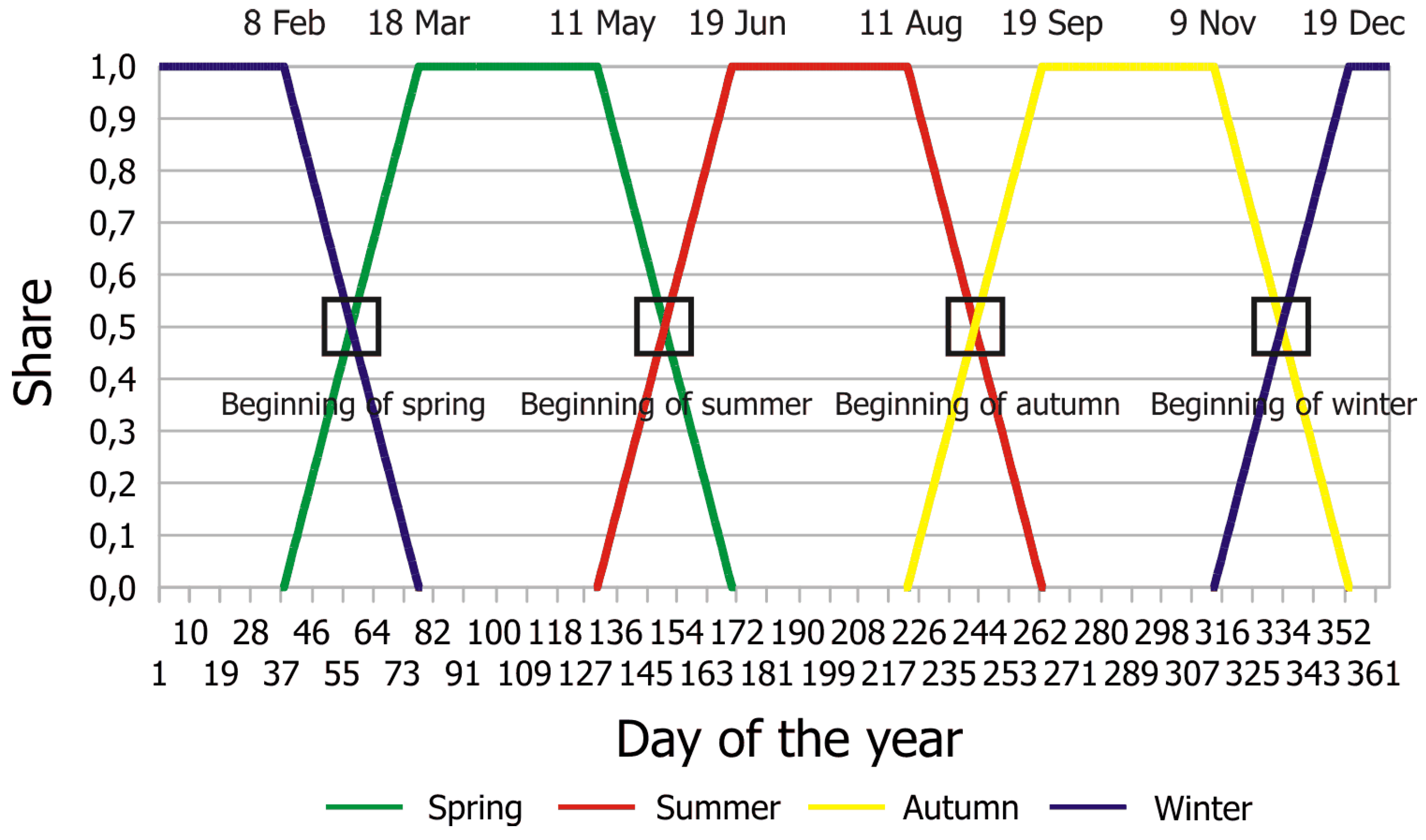
3.6. Reducing the Effects of Season Breaks

It is common to derive climate statistics on a fix temporal grid, e.g., the meteorological seasons or the hydrological half-years (winter half year⇁November-December-January-February-March-April (NDJFMA), summer half year⇁May-June-July-August-September-October (MJJASO)) or the vegetation period (April-May-June (AMJ)).
It appears to be consistent to use the same division for determining the temporal grid for the WG, e.g., the classification of the circulation patterns (cf. Section 2.2). In addition, the flow regime has a seasonal variability: for example, flow patterns that are in conjunction with high temperature in summer look much different from those associated with high temperature in winter [23].
In this Section, a rationale to stray from the strict adherence to a seasonally-specific approach is given. Furthermore, a methodology, implemented in the WETTREG WG, to avoid seasonal breaks is shown.
Imagine that the patterns/classes were derived strictly seasonally and the synthesized time series by the WG would approach the end of winter. On the last day of February, all the rules and the classification for winter would apply, and from the first day of March on, the respective set of boundary condition for spring would be governing the process. There is potential for an artificial break in the synthesized time series. Moreover, should an episode that starts in winter be arbitrarily cut off at the season’s end, to be continued by an episode that begins on the first day of the subsequent season? Again, there is a potential and artificial break to be, if not avoided, then at least diminished.
The solution in the WETTREG WG incorporates an initial generation of a seasonal classification. Then, for each day, the distance measure is not only computed (leading to the assignment to its most similar class) for “its” season, but the assignment is carried out to one of the classes in each of the other seasons, as well. For the optimization criteria during the selection process, a “handover process” is invoked. The idea is that around the middle of a season, the assignment of a day to its season—and its specific target frequency distribution of the circulation patterns—remains untouched, i.e., at a share of 1.0. In a zone of 20 days before and after the transition from one season to the next, the goodness-of-fit is gradually blended between the classification of both seasons with a linear decrease/increase of the weights, which always adds up to one, as shown in Figure 8.
Figure 8. Sketch of the priority of the season-specific class assignments over the year.
Atmosphere 04 00169 g008

4. From the WG to the Production of Local Time Series

It should be kept in mind that the WG is part of a downscaling method. Several aspects of this method had been briefly mentioned for contextual purposes in the course of this paper. The bulk of the described steps, however, was using local information, derived from measurements at stations, in an aggregated way. When pre-processing the surface data, areal averages were computed and applied, e.g., in the context of the definition of circulation patterns. Moreover, those aggregated surface data were used to define the pool of dates that determine the episodes that the WG assembles into synthesized time series.
As sketched in Figure 9, there is a straightforward way of arriving at local time series according to the sequence of dates that the WG produces. Since the WG is governed by the temporal evolution of circulation pattern frequency, the synthesized time series includes the signature of this evolution. Since scenario runs of a climate model are evaluated, the result is a set of local time series, which contain the signature of a changing climate. Moreover, the local time series from the investigation area are reflecting this signature in a coherent way, since the assembly rules are applied synchronously. In other words, ultimately, we arrive at a set of time series for the station locations wherein the local information is used, re-assembled according to a guidance that depends on processes on the large spatial scale.
The synthesized local time series can also be used to further assess the magnitude of the climate parameters at locations where no station is present. This is achieved by a height-dependent interpolation to these locations. Since this is beyond the mere application of the WG, only a sketch of one possible procedure is given here: At first, the height-dependency of the meteorological element is determined and removed. Secondly, a bilinear interpolation is carried out, followed by superimposing the height-dependency again. This approach is suitable for mean values, but for individual days, extremes and extreme indicators, such as threshold days, the results may be misleading.
Figure 9. Sketch of the context in which WETTREG applies the WG. Using the pool of dates (cf. Figure 5), specific episodes are selected and their sequence are prescribed by way of a criteria-driven rejection/acceptance process: the WG (top left panel). This prescription is then applied to identify the corresponding pieces from a time series of an example station Y (top right panel). Finally, for this and each other station, time series are generated in the prescribed sequence (bottom panel).
Atmosphere 04 00169 g009

5. Comparison to Other Methods

How does the WETTREG method compare to other downscaling approaches which apply WGs? Most of the related methods mentioned in Section 1 are used just for precipitation. Other methods, such as the UK Climate Projections (UKCIP) WG [39], are set up to describe single stations only. Due to those differences, a comparison is not feasible. The obvious opportunity for a comparison of downscaling methods would be to study results of RCM and ESM simulations. There are several studies of this kind for Germany and a number of German regions. These comparisons incorporate results from The Regional Model from the Max Planck Institute for Meteorology (REMO) [49], Community Climate Model (CCLM) [50] and STAR2 [19] simulations. Most of these studies are available as reports, i.e., not in peer-reviewed journals, e.g., [51,52,53]. A comparison for a subregion from Germany has been published in [24].
A common feature of all these comparisons is that numerous similarities, but also differences, could be identified. To improve the understanding of those differences, a research project (name: ReKliEs-De) (ReKliEs-De: Regionales Klimaszenarien Ensemble für Deutschland (Ensemble of regional climate scenarios Germany), funded by the German Ministry for Research and Education, has been set up. It will be launched in April 2013 and will include a systematic comparison of three RCMs (REMO, CCLM and Weather, research and Forecasting Model (WRF) [54]) with two ESDs (Statistical Analogue and Resampling Scheme (STARS) and WETTREG).

6. Remarks

6.1. Effects of the Changing Frequency of Circulation Patterns

As long as the frequency distribution of the patterns in a future time frame bears similarity to that from the current climate, the WG rather freely draws its episodes from the entire pool. Consequently, the target of meeting the projected frequency distribution of the patterns by way of assembling a sequence of present-time episodes is well met.
However, the future and the current frequency distribution of the patterns gradually drift apart. Certain patterns, associated with low temperature (i.e., strong negative temperature anomalies) vanish altogether, whereas the patterns that are linked to high temperature (i.e., strong positive temperature anomalies) and that are rare in current climate conditions become increasingly frequent. Broadly speaking, the frequency distribution changes its shape from normal to triangular; this was briefly mentioned in conjunction with Figure 3 in Section 3.
This behaviour is a challenge to the WG. To an increasing degree, i.e., associated with increasing time horizons, segments that contain ‘cold’ classes are left unused in the synthesizing process. Conversely, more and more episodes containing ‘warm’ classes (of which there are, unfortunately, only a few available in the pool) are in demand by the WG to meet the requirements prescribed by the development of the patterns’ frequency distribution over time, leading to (i) the frequent use of few episodes and (ii) a decreasing goodness-of-fit of the patterns’ distribution. The latter becomes more relevant when a further aspect is taken into consideration: the in-demand episodes are not entirely made of days with the required ‘very warm’ patterns, i.e., above pattern #9. Thus, there is always a kind of penalty that comes with the enforced inclusion of less required patterns, e.g., those associated with a mid-temperature range. This contributes to the decreasing goodness-of-fit described above.
Experimentally, several solution approaches have been introduced.
  • An extended database of episodes. The idea is based on the delta method. Using the observed time series, an additional set of episodes is generated. Due to the fact that the temperature (i) is causing the problem and (ii) is of high relevance, all temperature values will be increased by a certain value. If needs be, an adjustment of other weather elements is carried out to ensure physical consistency, for example, a higher temperature necessitates the adjustment of the water vapour pressure.
    To find an appropriate increment, the difference between the mean value of the neighbour temperature classes need to be determined. Based on the assigned class number, each temperature value receives a class-specific correction. Then, the class number, which was originally assigned to a day, needs to be stepped up by one (except for those days that were in the highest class already). The result is an “upward shift” in class membership without changing the value boundaries of the classes themselves (except for the topmost class). Consequently, the episodes in the pool then contain an increased number of days with high temperature class assignments.
    This has a physical rationale, because it can be argued that the same dynamic atmospheric conditions will be, in the future, linked, e.g., with a higher temperature range, making them the “more extreme relatives” of current patterns. If this alternative pool of shifted episodes is gradually allowed to be used towards the end of the 21st century, i.e., when the frequency of the patterns that needs to be met is gradually deforming, there will be two consequences: (i) the quite frequent usage of just a few episodes is reduced and (ii) an increase in the goodness-of-fit ensues.
  • A modified definition of the episodes. In the ‘standard’ version of the WG, an episode is beginning and ending with a zero-crossing, i.e., a transition from below-average to above-average conditions (or vice versa), as described in Section 3.2 and visualized in Figure 4. If the threshold is shifted upwards, episodes are allowed to occur that contain a smaller share of classes associated with rather low temperature ranges.
    The physical rationale would be that it can be argued that a future annual cycle might shift, as well. These episodes are clearly shorter than the ones derived the standard way; so, the minimum length criterion (cf. Section 3.2) needs to be taken into account. Introducing this measure has two consequences: (i) the effect caused by the introduction of excess days with patterns in the mid-range is reduced and (ii) an increase in the goodness-of-fit ensues.
Without losing the stochastical independence of the synthesized time series, a better representation of the modelled climate change is achieved through the above experimentations. This is particularly the case when the target frequency distributions prescribed by the models’s projected climate develop into a shape that is increasingly different from the one that characterizes the present-day climate. The caveat is that the statistical method, WETTREG, of which the WG is a core element, is then conditioned to a higher degree to follow the GCM-specific climate development at the risk of picking up a higher amount of GCM uncertainty.

6.2. Extremes

Therefore, the WG has synthesized local time series that bear the signature of large scale information, even the change of that information. However, it needs to be asked if these series would contain extremes. This will be examined below.
Owing to the fact that the WG re-shuffles episodes drawn from the current climate, new extremes in the resolution of the data, e.g., in the case of daily data, new daily precipitation records, will not be generated in the synthesized time series. With respect to precipitation, it needs to be pointed out that the selection/rejection criteria, which are rooted in the changing frequency of the patterns over time. call for repeated usage of a subset of the episodes (cf. Section 6.1). Consequentially, other episodes remain unused, particularly towards the longer time horizons, when the frequency of certain circulation patterns is increased in the GCM runs. Those patterns are associated, e.g., with a high temperature range, which is comparably rare in the current climate. It is probable that daily extremes, which might nevertheless occur in the episodes that are left out, could be overlooked.
However, depending on the classes to which the precipitation extremes are associated, the selection/rejection criteria can lead to an accumulation of precipitation, too. This may have consequences for (i) longer aggregations, such as monthly or seasonal precipitation, or (ii) the behaviour in the higher percentiles of the distribution and the frequency of surpassing extreme thresholds. Particularly, the latter behaviour applies to other climate elements (temperature, wind, etc.), as well.
As to the selection of thresholds, it needs to be acknowledged that events with a return time of, e.g., 40 years or longer cannot be inferred with confidence if the pool of observations itself contains on the order of 40 years. This also reduces the applicability of absolute minima and maxima, which are the respective 0- and 100-percentile of a distribution. It is recommended to relax the rigour and use 99-, 98- or 95-percentiles instead, which constitute more robust measures [31].

6.3. User Requirements vs. Deliver-Ability of a WG

Devising and developing a WG is a process subject to trade-offs. It is acknowledged that the user looks for qualities, such as high resolution, representativity, robustness, consistency across several climate parameters or the truthful representation of extremes, with respect to both their magnitude and duration. Moreover, the time series produced by the WG should contain a well-balanced proportion of randomness and (deterministic) modification, according to some external signal or target property. Last but not least, all these requirements should be met at once. Clearly, realizing such a “jack-of-all-trades” is next to impossible.
Some aspects of the WG were presented and discussed in the bulk of this paper. With respect to the problem at hand, i.e., “imprinting” the signature of climate change onto time series, it is an adequate approach to produce synthesized series that consist of sections of current climate. On the grounds that the set of rules that governs the selection/rejection procedure, according to large-scale circulation changes—which, in turn, GCMs can reproduce with consistency—a rather large number of the above requirements can be met by the presented WG.

7. Summary and Outlook

In the previous sections, we have given a description of a weather generator (WG), which is the heart of the statistical downscaling method WETTREG. It combines random sampling of episodes of measured climate from the present with a steering algorithm that governs the selection process according to the modelled changes in frequency of circulation patterns—according to 20C and scenario runs of a climate model. The result is a synthesized set of local time series of weather elements that represent a future climate state, as it is projected by the climate model.
Numerous assumptions, steps and considerations were introduced, explained and justified. Occasionally, alternative approaches and their consequences to the process of weather generation have been shown. It should be added that the development of the WG is an ongoing process and that this paper documents core ideas and implementations. The downscaling method, WETTREG, itself encompasses more than a decade of research and development. Frequently, the development stages were published in reports to the funding agencies (e.g., [25,28,29,55,56]). This was accompanied by peer reviewed papers (e.g., [23,24,26,27,41,57]) in which important aspects of the WETTREG method and its evolution can be found.
The authors acknowledge that users (e.g., impact modellers or decision makers) still have numerous requests and requirements, which to address need a constant and ongoing effort. This includes the wish to have WETTREG driven by a user-prescribed frequency distribution of circulation patterns in order to carry out climate sensitivity studies. Another field of interest is an improved inclusion of the occurrence of emerging new weather extremes.

Authors’ Contributions

W.E. and F.K. have developed the weather generator. F.K. included it into the operational processes of the WETTREG method. A.S. and F.K. compiled the paper, all authors discussed and corrected the paper. All authors read and approved the final manuscript.

Acknowledgments

The data from the climate stations are courtesy of the German Weather Service. NCEP Reanalysis data were provided by the NOAA/OAR/ESRL PSD, Boulder, Colorado, USA, through their web site. The ECHAM5/MPI-OM data were provided by the World Data Center for Climate, Hamburg, Germany, through their web site. The authors wish to thank the two reviewers for providing comments that added to the clarity of this paper.

Conflict of Interest

The authors declare no conflict of interest.

References

  1. Wilks, D. Use of stochastic weather generators for precipitation downscaling. WIREs Clim. Chang. 2010, 1, 898–907. [Google Scholar] [CrossRef]
  2. Semenov, M. Simulation of extreme weather events by a stochastic weather generator. Clim. Res. 2008, 35, 203–212. [Google Scholar] [CrossRef]
  3. Richardson, C. Stochastic simulation of daily precipitation, temperature, and solar radiation. Water Resour. Res. 1981, 17, 182–190. [Google Scholar] [CrossRef]
  4. Richardson, C.; Wright, D. WGEN: A Model for Generating Daily Weather Variables; Technical Report; USDA/ARS, ARS-8; Agricultural Research Service: Washington, DC, USA, 1984.
  5. Hantel, M.; Acs, F. Physical aspects of the weather generator. J. Hydrol. 1998, 212–213, 393–411. [Google Scholar] [CrossRef]
  6. Global International Geosphere–Biosphere Programme (IGBP) Change. Available online: www.igbp.net (accessed on 31 May 2013).
  7. Bass, B. BAHC Focus 4: The Weather Generator Project; Technical Report; BAHC Report No. 4; BAHC Core Project Office, Freie Universität Berlin: Berlin, Germany, 1994. [Google Scholar]
  8. Waymire, E.; Gupta, V. The mathematical structure of rainfall representations—1. A review of the stochastic rainfall models. Wat. Resour. Res. 1981, 17, 1261–1272. [Google Scholar] [CrossRef]
  9. Katz, R.; Parlange, M. Mixtures of stochastic processes: Application to statistical downscaling. Clim. Res. 1996, 7, 185–193. [Google Scholar] [CrossRef]
  10. Gabriel, K.; Neumann, J. A Markov chain model for daily rainfall occurrence at Tel Aviv. Quart. J. Roy. Met. Soc. 1962, 88, 90–95. [Google Scholar] [CrossRef]
  11. Todorovic, P.; Woolhiser, D. A stochastic model of n-day precipitation. J. Appl. Meteorol. 1975, 14, 17–24. [Google Scholar] [CrossRef]
  12. Busuioc, A.; von Storch, H. Conditional stochastic model for generating daily precipitation time series. Clim. Res. 2003, 24, 181–195. [Google Scholar] [CrossRef]
  13. Wilks, D. Adapting stochastic weather generation algorithms for climate change studies. Clim. Res. 1992, 22, 67–84. [Google Scholar] [CrossRef]
  14. Semenov, M.; Barrow, E. Use of a stochastic weather generator in the development of climate change scenarios. Clim. Change 1997, 35, 397–414. [Google Scholar] [CrossRef]
  15. Schubert, S. A weather generator based on the European “Grosswetterlagen”. Clim. Res. 1994, 4, 191–202. [Google Scholar] [CrossRef]
  16. Gerstengarbe, F.; Werner, P. Katalog der Großwetterlagen Europas (1881–2004) nach P. Hess und H. Brezowsky; Technical Report 100; PIK-Reports; Potsdam Institut für Klimafolgenforschung: Potsdam, Germany, 2005. [Google Scholar]
  17. Corte-Real, J.; Xu, H.; Qian, B. A weather generator for obtaining daily precipitation scenarios based on circulation patterns. Clim. Res. 1999, 13, 61–75. [Google Scholar] [CrossRef]
  18. Wilks, D.; Wilby, R. The weather generation game: A review of stochastic weather models. Progr. Phys. Geogr. 1999, 23, 329–357. [Google Scholar] [CrossRef]
  19. Orlowsky, B.; Gerstengarbe, F.W.; Werner, P. A resampling scheme for regional climate simulations and its performance compared to a dynamical RCM. Theor. Appl. Climatol. 2008, 92, 209–223. [Google Scholar] [CrossRef]
  20. Hayhoe, H. Improvements of stochastic weather data generators for diverse climates. Clim. Res. 2000, 14, 75–87. [Google Scholar] [CrossRef]
  21. Mason, S. Simulating climate over Western North America using stochastic weather generators. Clim. Change 2004, 62, 155–187. [Google Scholar] [CrossRef]
  22. Bárdossy, A.; Pegram, G. Copula based multisite model for daily precipitation simulation. Hydrol. Earth Syst. Sci. 2009, 13, 2299–2314. [Google Scholar] [CrossRef]
  23. Spekat, A.; Kreienkamp, F.; Enke, W. An impact-oriented classification method for atmospheric patterns. Phys. Chem. Earth 2010, 35, 352–359. [Google Scholar] [CrossRef]
  24. Kreienkamp, F.; Baumgart, S.; Spekat, A.; Enke, W. Climate signals on the regional scale derived with a statistical method: Relevance of the driving model’s resolution. Atmosphere 2011, 2, 129–145. [Google Scholar] [CrossRef]
  25. Enke, W.; Spekat, A. Verbundprojekt: Klimavariabilität und Signalanalyse. Teilthema: Signalanalyse zur Regionalisierung von Klimamodell-Outputs mit Hilfe der Erkennung Synoptischer Muster und Statistischer Analysemethoden; Technical Report 07KV01/1 (161/30); Bundesministerium für Bildung und Forschung (BMBF): Bonn, Germany, 1994. [Google Scholar]
  26. Enke, W.; Spekat, A. Downscaling climate model outputs into local and regional weather elements by classification and regression. Clim. Res. 1997, 8, 195–207. [Google Scholar] [CrossRef]
  27. Enke, W.; Deutschländer, T.; Schneider, F.; Küchler, W. Results of five regional climate studies applying a weather pattern based downscaling method to ECHAM4 climate simulations. Meteorol. Z. 2005, 14, 247–257. [Google Scholar] [CrossRef]
  28. Spekat, A.; Enke, W.; Kreienkamp, F. Neuentwicklung von regional hoch aufgelösten Wetterlagen für Deutschland und Bereitstellung Regionaler Klimaszenarios auf der Basis von Globalen Klimasimulationen mit dem Regionalisierungsmodell WETTREG auf der Basis von Globalen Klimasimulationen mit ECHAM5/MPI-OM T63L31 2010 bis 2100 für die SRES-Szenarios B1, A1B und A2 (Endbericht). Im Rahmen des Forschungs- und Entwicklungsvorhabens: Klimaauswirkungen und Anpassungen in Deutschland—Phase I: Erstellung regionaler Klimaszenarios für Deutschland des Umweltbundesamtes; Technical Report Förderkennzeichen 204 41 138; Umweltbundsamt, Dessau, 2007. [Google Scholar]
  29. Kreienkamp, F.; Spekat, A.; Enke, W. Weiterentwicklung von WETTREG Bezüglich Neuartiger Wetterlagen; Technical Report. CEC-Potsdam on Behalf of a Consortium of Environment Agencies from German Federal States, 2010. Available online: klimawandel.hlug.de/fileadmin/dokumente/klima/inklim_a/TWL_Laender.pdf (accessed on 31 May 2013).
  30. Mehrotra, R.; Sharma, A. Evaluating spatio-temporal representations in daily rainfall sequences from three stochastic multi-site weather generation approaches. Adv. Wat. Res. 2009, 32, 948–962. [Google Scholar] [CrossRef]
  31. Kreienkamp, F.; Hübener, H.; Linke, C.; Spekat, A. Good practice for the usage of climate model simulation results—A discussion paper. Env. Syst. Res. 2012, 1, 9–37. [Google Scholar] [CrossRef]
  32. Kalnay, E.; Kanamitsu, M.; Kistler, R.; Collins, W.; Deaven, D.; Gandin, L.; Iredell, M.; Saha, S.; White, G.; Woollen, J.; et al. The NCEP/NCAR 40-year reanalysis project. Bull. Amer. Met. Soc. 1996, 77, 437–471. [Google Scholar] [CrossRef]
  33. Uppala, S.M.; Kållberg, P.W.; Simmons, A.J.; Andrae, U.; da Costa Bechtold, V.; Fiorino, M.; Gibson, J.K.; Haseler, J.; Hernandez, A.; Kelly, G.; et al. The ERA-40 re-analysis. Quart. J. Roy. Met. Soc. 2005, 131, 2961–3012. [Google Scholar] [CrossRef]
  34. Dee, D.; Uppala, S.; Simmons, A.; Berrisford, P.; Poli, P.; Kobayashi, S.; Andrae, U.; Balmaseda, M.; Balsamo, G.; Bauer, P.; et al. The ERA-Interim reanalysis: Configuration and performance of the data assimilation system. Quart. J. Roy. Met. Soc. 2011, 137, 553–597. [Google Scholar] [CrossRef]
  35. Woods, A. Medium-Range Weather Prediction—The European Approach. The Story of the European Center for Medium-Range Weather Forecasts; Springer: New York, NY, USA, 2006. [Google Scholar]
  36. Edwards, P. A Vast Machine—Computer Models, Climate Data, and the Politics of Global Warming; MIT Press: Cambridge, MA, USA, 2010. [Google Scholar]
  37. Nakićenović, N.; Alcamo, J.; de Vries, B.; Fenhann, J.; Gaffin, S.; Gregory, K.; Grübler, A.; Jung, T.; Kram, T.; Rovere, E.L.; et al. Emissions Scenarios; A Special Reports of IPCC Working Group III; Cambridge University Press: Cambridge, UK, 2000; p. 570. [Google Scholar]
  38. Moss, R.; Babiker, M.; Brinkman, S.; Calvo, E.; Carter, T.; Edmonds, J.; Elgizouli, I.; Emori, S.; Erda, L.; Hibbard, K.; Jones, R.; et al. Towards New Scenarios for Analysis of Emissions, Climate Change, Impacts, and Response Strategies. In Proceedings of Expert Meeting Report, Noordwijkerhout, The Netherlands, 19–21 September 2007; p. 132.
  39. Jones, P.; Kilsby, C.; Harpham, C.; Glenis, V.; Burton, A. UK Climate Projections Science Report: Projections of Future Daily Climate for the UK from the Weather Generator; Technical Report; University of Newcastle: Newcastle, UK, 2009. [Google Scholar]
  40. Benestad, R.; Hanssen-Bauer, I.; Cheng, D. Empirical-Statistical Downscaling; World Scientific Publishing Co. Pte. Ltd.: Singapore, Singapore, 2008. [Google Scholar]
  41. Enke, W.; Schneider, F.; Deutschländer, T. A novel scheme to derive optimized circulation pattern classifications for downscaling and forecast purposes. Theor. Appl. Climatol. 2005, 82, 51–63. [Google Scholar] [CrossRef]
  42. Christensen, J.H. Prediction of Regional Scenarios and Uncertainties for Defining European Climate Change Risks and Effects (PRUDENCE), Final Report; Technical Report EVK2-CT2001-00132; Danish Meteorological Institute (DMI): Copenhagen, Denmark, 2005. [Google Scholar]
  43. Yarnal, B. Synoptic Climatology in Environmental Analysis; Belhaven Press: London, UK, 1993. [Google Scholar]
  44. Philipp, A.; Bartholy, J.; Beck, C.; Erpicum, M.; Esteban, P.; Huth, R.; James, P.; Jourdain, S.; Krennert, T.; et al. COST733CAT—A database of weather and circulation type classifications. Phys. Chem. Earth 2010, 35, 360–373. [Google Scholar] [CrossRef]
  45. Huth, R. Synoptic-climatological applicability of circulation classifications from the COST733 collection: First results. Phys. Chem. Earth 2010, 35, 388–394. [Google Scholar] [CrossRef]
  46. Roeckner, E.; Baeuml, G.; Bonaventura, L.; Brokopf, R.; Esch, M.; Giorgetta, M.; Hagemann, S.; Kirchner, I.; Kornblueh, L.; Manzini, E.; et al. The Atmospheric General Circulation Model ECHAM5—Part 1: Model Description; Report No. 349, MPI-Berichte; Max-Planck-Institut für Meteorologie: Hamburg, Germany, 2003. [Google Scholar]
  47. Roeckner, E.; Brokopf, R.; Esch, M.; Giorgetta, M.; Hagemann, S.; Kornblueh, L.; Manzini, E.; Schlese, U.; Schulzweida, U. The Atmosphere General Circulation Model ECHAM5—Part 2: Sensitivity of Simulated Climate to Horizontal and Vertical Resolution; Report No. 354, MPI-Berichte; Max-Planck-Institut für Meteorologie: Hamburg, Germany, 2004. [Google Scholar]
  48. World Meteorological Organization (WMO). Guide to Climatological Practices, 3rd ed.; Technical Report (WMO-No. 100); WMO: Geneva, Switzerland, 2010. [Google Scholar]
  49. Regional Climate Modelling. Available online: www.remo-rcm.de (accessed on 31 May 2013).
  50. Climate Limited-Area Modelling COmmunity. Available online: www.clm-community.eu (accessed on 31 May 2013).
  51. Linke, C.; Grimmert, S.; Hartmann, I.; Reinhardt, K. Auswertung Regionaler Klimamodelle für das Land Brandenburg; Technical Report; Fachbeiträge des Landesumweltamtes, Heft 113; Ministerium für Umwelt, Gesundheit und Verbraucherschutz: Land Brandenburg, Germany, 2010. [Google Scholar]
  52. Linke, C.; Grimmert, S.; Hartmann, I.; Reinhardt, K. Auswertung Regionaler Klimamodelle für das Land Brandenburg. Teil 2; Technical Report; Fachbeiträge des Landesumweltamtes, Heft 115; Ministerium für Umwelt, Gesundheit und Verbraucherschutz: Land Brandenburg, Germany, 2010. [Google Scholar]
  53. Arbeitskreis KLIWA. Regionale Klimaszenarien für Süddeutschland. Abschätzung der Auswirkungen auf den Wasserhaushalt. Technical Report; LUBW, KLIWA-Berichte Heft 9. 2006. Available online: http://www.kliwa.de/download/KLIWAHeft9.pdf (accessed on 31 May 2013).
  54. The Weather Research and Forecasting Model. Available online: www.wrf-model.org (accessed on 31 May 2013).
  55. Kreienkamp, F.; Spekat, A.; Enke, W. Ergebnisse eines regionalen Szenarienlaufs für Deutschland mit dem statistischen Modell WETTREG2010; Technical Report; Climate and Environment Consulting Potsdam GmbH im Auftrag des Umweltbundesamtes: Dessau, Germany, 2010. [Google Scholar]
  56. Kreienkamp, F.; Spekat, A.; Enke, W. Ergebnisse Regionaler Szenarienläufe für Deutschland mit der Statistischen Methode WETTREG auf der Basis der SRES Szenarios A2 und B1 Modelliert mit ECHAM5/MPI-OM; Technical Report; Climate and Environment Consulting Potsdam GmbH, Climate Service Center: Hamburg, Germany, 2011. [Google Scholar]
  57. Kreienkamp, F.; Spekat, A.; Enke, W. Sensitivity studies with a statistical downscaling method—The role of the driving large scale model. Meteorol. Z. 2009, 18, 597–606. [Google Scholar] [CrossRef] [PubMed]

