Communication

Variance of Fluctuating Radar Echoes from Thermal Noise and Randomly Distributed Scatterers

MeteoSwiss, via ai Monti 146, CH-6605 Locarno, Switzerland
Atmosphere 2014, 5(1), 92-100; https://doi.org/10.3390/atmos5010092
Submission received: 12 December 2013 / Revised: 23 January 2014 / Accepted: 29 January 2014 / Published: 20 February 2014
(This article belongs to the Special Issue Cloud and Precipitation)

Abstract

:
In several cases (e.g., thermal noise, weather echoes, …), the incoming signal to a radar receiver can be assumed to be Rayleigh distributed. When estimating the mean power from the inherently fluctuating Rayleigh signals, it is necessary to average either the echo power intensities or the echo logarithmic levels. Until now, it has been accepted that averaging the echo intensities provides smaller variance values, for the same number of independent samples. This has been known for decades as the implicit consequence of two works that were presented in the open literature. The present note deals with the deriving of analytical expressions of the variance of the two typical estimators of mean values of echo power, based on echo intensities and echo logarithmic levels. The derived expressions explicitly show that the variance associated to an average of the echo intensities is lower than that associated to an average of logarithmic levels. Consequently, it is better to average echo intensities rather than logarithms. With the availability of digital IF receivers, which facilitate the averaging of echo power, the result has a practical value. As a practical example, the variance obtained from two sets of noise samples, is compared with that predicted with the analytical expression derived in this note (Section 3): the measurements and theory show good agreement.

1. Introduction

When interpreting a fluctuating echo from a randomly distributed target, the usual problem is to estimate the long-term mean echo power, in order to obtain an estimate of the scatterers contained in the volume sampled by the radar pulse (e.g., Doviak and Zrnic [1]). In the case of weather targets, since scatterers move with respect to each other as a result of turbulence, shear and varying terminal fall velocities, their radar echo fluctuates from one echo to the next. Thus, the problem arises of estimating the mean echo power from the volume observed, on the basis of a certain number of echoes. This problem has been investigated since the beginning of radar meteorology, see e.g., Marshall and Hitschfeld [2], Wallace [3] and Smith [4], among others. The aim of the present note is to demonstrate, in closed form, that averaging the echo intensities in the radar receiver (i.e., averaging samples proportional to the square of the amplitude of the receiver signal) to obtain the mean echo power is more advantageous than averaging echo logarithmic levels (i.e., averaging samples proportional to the logarithm of the echo amplitude), since the estimate of the mean echo power that is based on the former method has a lower variance.
The derived formulas can also be useful to estimate the variance of radar receiver thermal noise, given the number of averaged samples. Prior to the envelop detector (rectification), which means energy detection in the electronic circuit, receiver thermal noise is expected to have a Gaussian distribution with a zero mean. After rectification, noise has an exponential one-sided probability distribution that fluctuates around a mean, which is the root-mean-squared value of the unrectified fluctuations. In other words, the results by Marshall and Hitschfeld [2], which were related to the treatise on sound by Lord Rayleigh [5], also apply to the thermal noise of the receiver. Actually, the assumption of Rayleigh fluctuations for thermal noise is probably even less controversial than for precipitation scatterers: the assumption of “all nearly equal scatterers” (i.e., no few scatterers dominate) for hydrometeors, in fact, requires “near statistical stationarity” or, equivalently, “near statistical homogeneity” of the hydrometeors in space. Furthermore, in the case of thermal noise, it is possible to assume that the number of available samples, M, coincides with the equivalent number of independent samples, N, which, throughout this note, has been used to express, in a simple way, the reduction in estimate variance that can be achieved by averaging. However, in the case of weather echoes, a considerable correlation may exist from sample to sample and with the typical pulse repetition frequency of meteorological radar. For example, Doviak and Zrnic (Section 6.3.1.2) [1], presented the variance reduction factor for the square-law receiver as a function of the raindrop Doppler velocity spectrum width, the unambiguous velocity, and the total number of weighted samples, M.
Section 2 briefly shows the mathematical background at the basis of the problem (Rayleigh scattering), while Section 3 shows that the variance of the estimator, associated to the average of intensities, is lower than that associated to the average of power levels on a logarithmic scale. Finally, a practical example and application of the derived analytical formulas are presented in Section 4, which deals with real noise data derived from a civil marine radar.

2. Signal Statistics of Meteorological Targets and Noise

It has been shown (Kerr and Goldstein [6]) that the probability density function of the power p from Rayleigh scatterers can be modeled by means of an exponential distribution, namely
Atmosphere 05 00092 i001
where p0 is a parameter that characterizes the exponential decay rate and which is coincident with the mean and standard deviation of the distribution; u(x) is the so-called step function, which is defined as 1 if x ≥ 0, and 0 otherwise. Because of the broad dynamic range of the power that has to be detected by a radar, it is often convenient to measure its logarithm compared to a reference power Pm; logarithmic amplifiers are used for this purpose. In what follows, the reference value pm has been chosen to be equal to 1 mW and a decimal logarithmic scale is used. Consequently, the logarithmic power level L is expressed in dBm, namely L = 10 Log(p/pm), where pm = 1 mW and [L] = dBm.
The probability density function of the logarithmic power level L is (see Wallace [3]):
Atmosphere 05 00092 i002
where the most probable value, L0, is coincident with the mean power E{P} = P0, once it is expressed on a decimal logarithmic scale and multiplied by 10; in other words, the most probable value, L0, is the mean power expressed in dBm:
L0=10 × Log(E{P}/Pm)=10∙Log(P0/Pm)
As shown in the sketch presented on page 966 in Marshall and Hitschfeld [2], in the 1st column and 4th row of Table 1, the logarithmic transformation applied to the exponential distribution causes fL(L) to be left-skewed. As can be seen in the 4th column and 4th row of the above-mentioned Table 1, the most probable value, L0, is 2.51 dB larger than the mean logarithmic power level, regardless of the mean power value p0. While the standard deviation that characterizes the probability distribution function fP(p) coincides with the mean power that is p0, the standard deviation of the probability distribution function fL(L) is independent of it. After logarithmic amplification, an increased mean power simply means a “rigid”, right-shift of the curve fL(L); furthermore, the standard deviation of a single radar echo, characterized by Rayleigh fluctuation (thermal noise, randomly distributed scatterers, …), has an intrinsic value of 5.57 dB (see next Section 3). In order to reduce this variance, N independent samples can be averaged: Is it better to average intensities or logarithmic levels? In both cases the variance of the estimator decreases as 1/N. As we will show in Section 3 (with the help of Appendix), averaging (power) intensities always leads to smaller variances.

3. The Estimators

On the basis of the two kinds of samples, namely intensity, pi, and logarithmic level, Lj, two estimators of the mean echo power can be constructed. The estimator based on the intensity samples, pi, is
Atmosphere 05 00092 i003
where the braces {}ML indicate that this estimator is the maximum-likelihood one. The estimator based on the logarithmic level samples, Lj, is
Atmosphere 05 00092 i004
where the 2.51 dBm term is introduced to obtain an unbiased estimator (see Section 2, just after Equation (3)). As the braces in Equation (4) indicate, P0 is estimated in dBm.
The uncertainty in the estimates of the mean echo power, starting from intensity or logarithmic level samples, is quantified by determining which of the two estimators has the smaller variance. Since the two estimators are for different (although directly related) parameters, the dBm value of the estimator in Equation (4) is computed:
Atmosphere 05 00092 i005
The performance index 2 σ/E is computed as a criterion for comparing the estimators in Equations (5) and (6), where E is the average value of the estimator and σ is its standard deviation. This means that the performance index characterizes the relative uncertainty of the estimator and is related to the confidence intervals normalised to the mean value. It is shown, in the Appendix, that the mean values of the estimators in Equations (5) and (6) are
EL = 10 × Log(P0/Pm)
and
Atmosphere 05 00092 i006
where Λ is Euler’s constant (Gradshtein and Ryzhik [7]).
The standard deviation of the estimators in Equations (5) and (6) are
Atmosphere 05 00092 i007
and
Atmosphere 05 00092 i008
Equation (7) tends to Equation (8) for large values of N; from an operational viewpoint, a direct comparison between σML and σL is particularly meaningful in the central part of Figure 1, with N ranging from 5 to 50) A comparison between the standard deviation of the two estimators is still possible for small values of N, as long as the known bias in Equation (8), the 1st term, is removed. As Figure 1 shows, the ML estimator has a smaller standard deviation for any number of independent samples, N. This result is not new: Similar conclusions can be derived from Figure 2 in the paper by Zrnic [8]; however, to the best of our knowledge, this note for the first time presents the analytical expressions for both, σML and σL (as well as their derivation in Appendix). In the next Section, these formulas are applied to two large sample radar noise measurement data sets: The retrieved values from the ensembles are consistent with those predicted by the theory.
Figure 1. Expected standard deviation from an ensemble of N independent samples of Rayleigh-distributed echoes. When the power is linearly averaged, the corresponding variance (dB scale), is smaller than the variance obtained by averaging power on a decibel (dB) scale. In the picture, N, spans from 2 to 200. As can be seen from both Equations (8) and (10), when N → 1, the intrinsic uncertainty tends to 5.57 dB.
Atmosphere 05 00092 g001

4. An Example Based on Noise Measurements from a Civil Marine Radar

As a practical example of Rayleigh-distributed (in amplitude, hence exponential-distributed in power) signals, radar noise measurements have been analyzed at the output of a radar receiver. The principal contribution at weather radar frequencies is found to be receiver thermal noise. Prior to the envelop detector (rectification), which means energy detection in the electronic circuit, receiver thermal noise is expected to have a Gaussian distribution with a zero mean. After rectification, the noise has an exponential one-sided probability distribution, fluctuating around a mean that is the root-mean-squared value of the unrectified fluctuations. Both presented data sets have been derived from the output of a low-cost and easily achievable civil marine radar. The main features of the system are described in Table 1 of the paper by Gabella et al. [9]. The present analysis is based on two sets made of slightly more than ten thousands noise measurements derived once per minute (one week of data). The standard deviation of these two noise measurement sets resulted to be 0.13 dB and 0.12 dB, respectively. Are such average values of the two realizations consistent with the mathematical prediction obtained in Section 3? Before answering this question, it is necessary to describe, in more detail, how the time-averaged, 1-minute-sampled noise measurements were derived: 8 contiguous pulses at far ranges (and at the zenith) were acquired for 9 consecutive shots: the 8 contiguous pulses were separated by the pulse length, which is 400 ns; the 9 consecutive shots are separated by the pulse repetition time, which is 1,250 μs. The antenna performs 22 revolutions each minute; however, only data from the first 16 revolutions (out of 22) were averaged on a linear power scale (algebraic average: dBm values are antilog transformed, then averaged, then transformed again on a decibel logarithmic scale). We assume that all such noise samples were independent. This would mean N = 1,152 (8 times 9 times 16) independent samples. If the noise measurements were the results of averaging logarithmic levels (geometric average), then the expected standard deviation would be 5.57/1,1520.5 = 0.16 dB, as can easily be derived from Equation (10). However, this is not the case, since it is known that intensities were averaged (algebraic average). Consequently, in order to predict the expected standard deviation, we would better use Equation (8), which in fact gives 0.13 dB. This value of standard deviation is much closer to those which were derived using the two civil marine radar experimental data sets.

5. Conclusions

When the incoming signal envelope to a radar receiver is Rayleigh-distributed, how is the variance reduced by the geometric or algebraic average of N independent samples? Analytical expressions of the variance of the two estimators have been given, and these have enabled a quantitative comparison to have been made between them. Confirming previous studies, we find that averaging echo intensities, rather than echo logarithmic levels, leads to smaller variance.

List of Symbols

In order of appearance in the text:
M
Total number of available samples.
N
Equivalent number of independent samples.
P
Echo power.
P0
Mean echo power.
u(x)
Step function, defined as 1 if x ≥ 0, and 0 otherwise.
L
Power logarithmic Level in dBm (that is, the reference value is set to 1 mW)
ln(x)
Natural logarithm of x.
L0
Level of the mean echo power.
Log(x)
Base-10 logarithm of x.
Pi
Echo power sample.
Li
Level of the echo power sample (dBm).
{β}ML
Maximum likelihood estimate of the parameter β.
E
Mean value of an estimator.
σ
Standard deviation of an estimator.
EML
Mean value of the Log-transformed ML estimator.
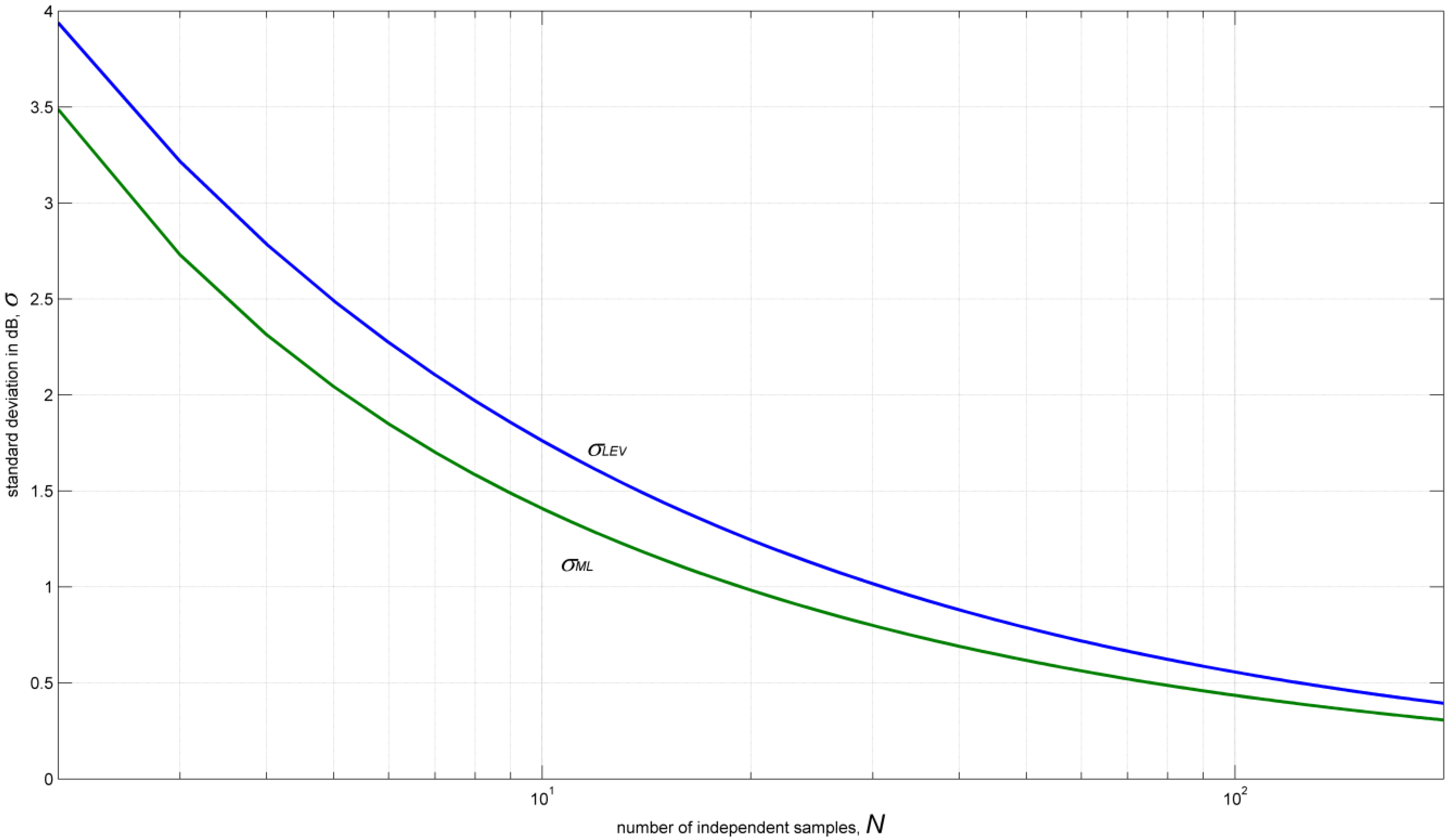
σML
Standard deviation of the Log-transformed ML estimator.
EL
Mean value of the level samples based estimator
σL
Standard deviation of the level samples based estimator.
Λ
Euler’s constant.
ζ(p,q)
Riemann’s zeta function.

Acknowledgments

The author is grateful to Jürg Joss for his valuable help in estimating the standard deviation of the two noise measurement sets, which consist of 10,416 samples, with a 0.4 dB quantization. He also would like to thank Maurizio Sartori, Dennis Vollbracht and Olivier Progin for interesting discussions regarding fluctuating radar echoes from thermal noise.

Conflicts of Interest

The author declares no conflict of interest.

References

  1. Doviak, R.J.; Zrnic, D.S. Doppler Radar and Weather Observations, 2nd ed.; Academic Press: Waltham, MA, USA, 1993. [Google Scholar]
  2. Marshall, J.S.; Hitschfeld, W. Interpretation of the fluctuating echoes from randomly distributed scatterers, Part I. Can. J. Phys. 1953, 31, 962–994. [Google Scholar] [CrossRef]
  3. Wallace, P.R. Interpretation of the fluctuating echoes from randomly distributed scatterers, Part II. Can. J. Phys. 1953, 31, 995–1009. [Google Scholar] [CrossRef]
  4. Smith, P.L. Interpretation of the Fluctuating Echo from Randomly Distributed Scatterers, Part III. In Proceedings of the 12th Conference on Radar Meteorology, Norman, OK, USA, 17–20 October, 1966.
  5. Rayleigh, J.W.S.B. The Theory of Sound; Macmillan: London, UK, 1877; Volume I, Reprinted version, in 1945 by Dover Publications; p. 984. [Google Scholar]
  6. Kerr, D.E.; Goldstein, H. Radar Target and Echoes. In Propagation of Short Radio Waves, 2nd ed.; Kerr, D.E., Ed.; Peter Peregrinus Ltd. on behalf of The Institution of Electrical Engineers: Stevenage, UK, 1987. [Google Scholar]
  7. Gradshteyn, I.S.; Ryzhik, I.M. Tables of Integrals, and Products; Academic Press: Waltham, MA, USA, 1980; p. 1156. [Google Scholar]
  8. Zrnic, D.S. Moments of estimated input power for finite sample averages of radar receiver outputs. IEEE Trans. Aerosp. Electron. Syst. 1975, 11, 109–113. [Google Scholar] [CrossRef]
  9. Gabella, M.; Notarpietro, R.; Turso, S.; Perona, G. Simulated and measured X-band radar reflectivity of land in mountainous terrain using a fan-beam antenna. Int. J. Remote Sens. 2008, 29, 2869–2878. [Google Scholar] [CrossRef]

Appendix

A1. Mean and Variance of the Log-Transformed Maximum Likelihood Estimator

We obtain the standard deviation of the estimator {10 × Log(P0/Pm)} in Equation (6).
We know that the random variable in Equation (4) has the following distribution of probability (see Wallace [3]; u(x) is the step function, see also list of symbols at the end ):
Atmosphere 05 00092 i009
since the random variable obtained by Log-transformation (base-10 Logarithm) has the following probability distribution function:
Atmosphere 05 00092 i010
then we can conclude then that the estimator Atmosphere 05 00092 i011 has the following probability distribution function:
Atmosphere 05 00092 i012
Hence the standard deviation of the right therm in Equation (6) will be Atmosphere 05 00092 i013, where:
Atmosphere 05 00092 i014

A2. Computation of I1

We have:
Atmosphere 05 00092 i015
substituting in Equation (A6) ρ = 10x and using Equation (4.352.1) in Gradshteyn and Ryzhik [7], page 576, we obtain that:
Atmosphere 05 00092 i016
where Λ = Euler’s constant (Gradshteyn and Ryzhik [7], Equation (8.367.1) page 946).

A3. Computation of I2

Since:
Atmosphere 05 00092 i017
substituting again ρ = 10x in the above-listed equation and using (see Gradshteyn and Ryzhik [7], Equation (4.538.2) page 578, Equations (8.365) and (8.366) page 945, and Equation (8.339.1) page 938) we obtain:
Atmosphere 05 00092 i018
where (see Gradhstein and Ryzhik [7], Equation (4.251.4) page 537 and Equation (8.366.11) page 946).
Atmosphere 05 00092 i019

A4. Conclusions

From Equations (A7), (A9) and (A10) we conclude that the estimator in Equation (6) has the following mean and variance:
Atmosphere 05 00092 i020
Atmosphere 05 00092 i021

