Air-Sea Exchange of Legacy POPs in the North Sea Based on Results of Fate and Transport, and Shelf-Sea Hydrodynamic Ocean Models

Abstract
:1. Introduction
2. Modeling System
2.1. Model Description
2.1.1. Model Configuration

2.1.2. HAMSOM
2.1.3. FANTOM


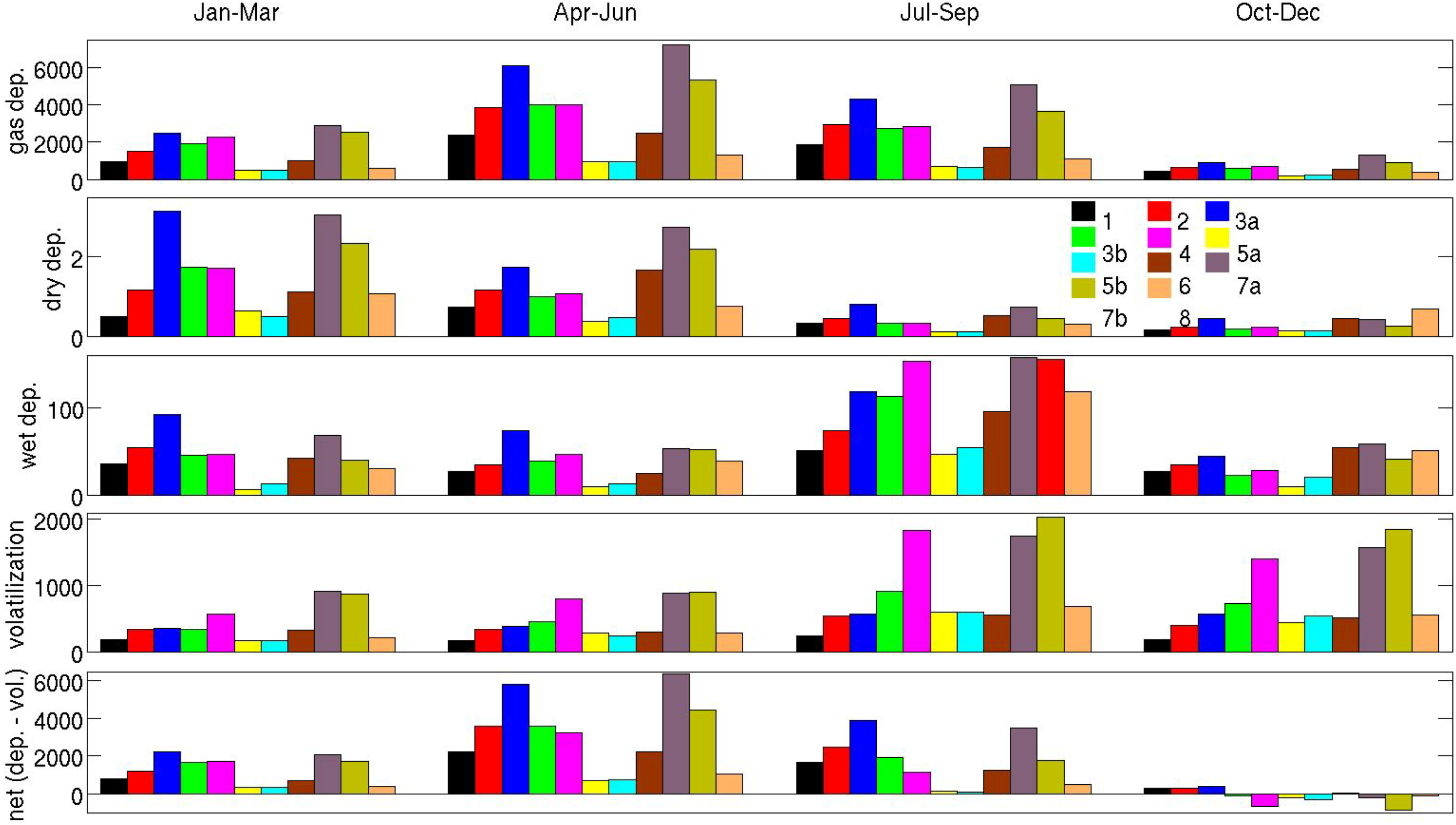
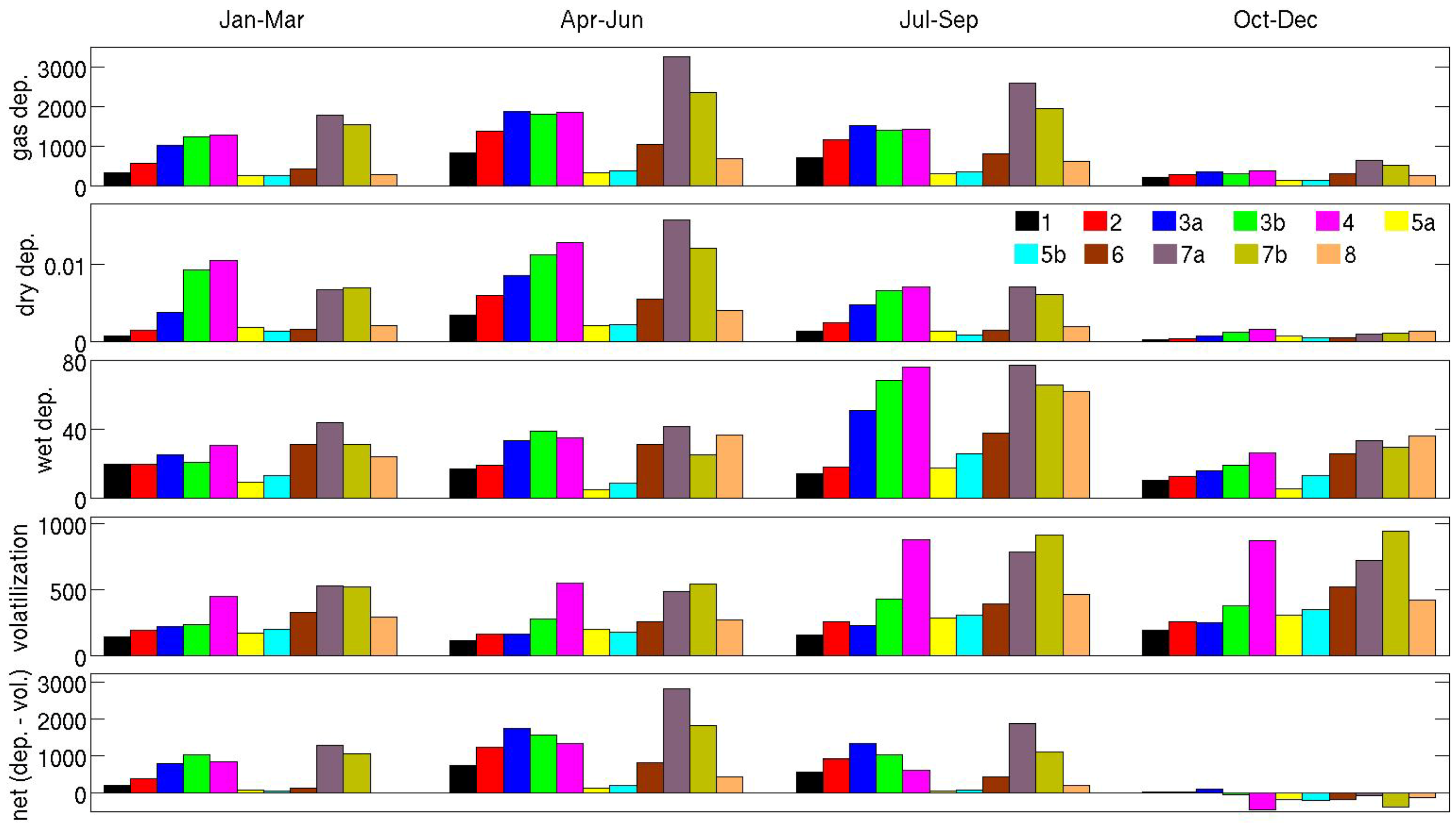
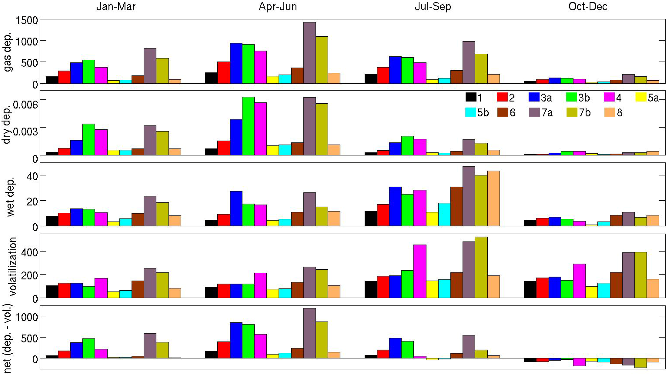
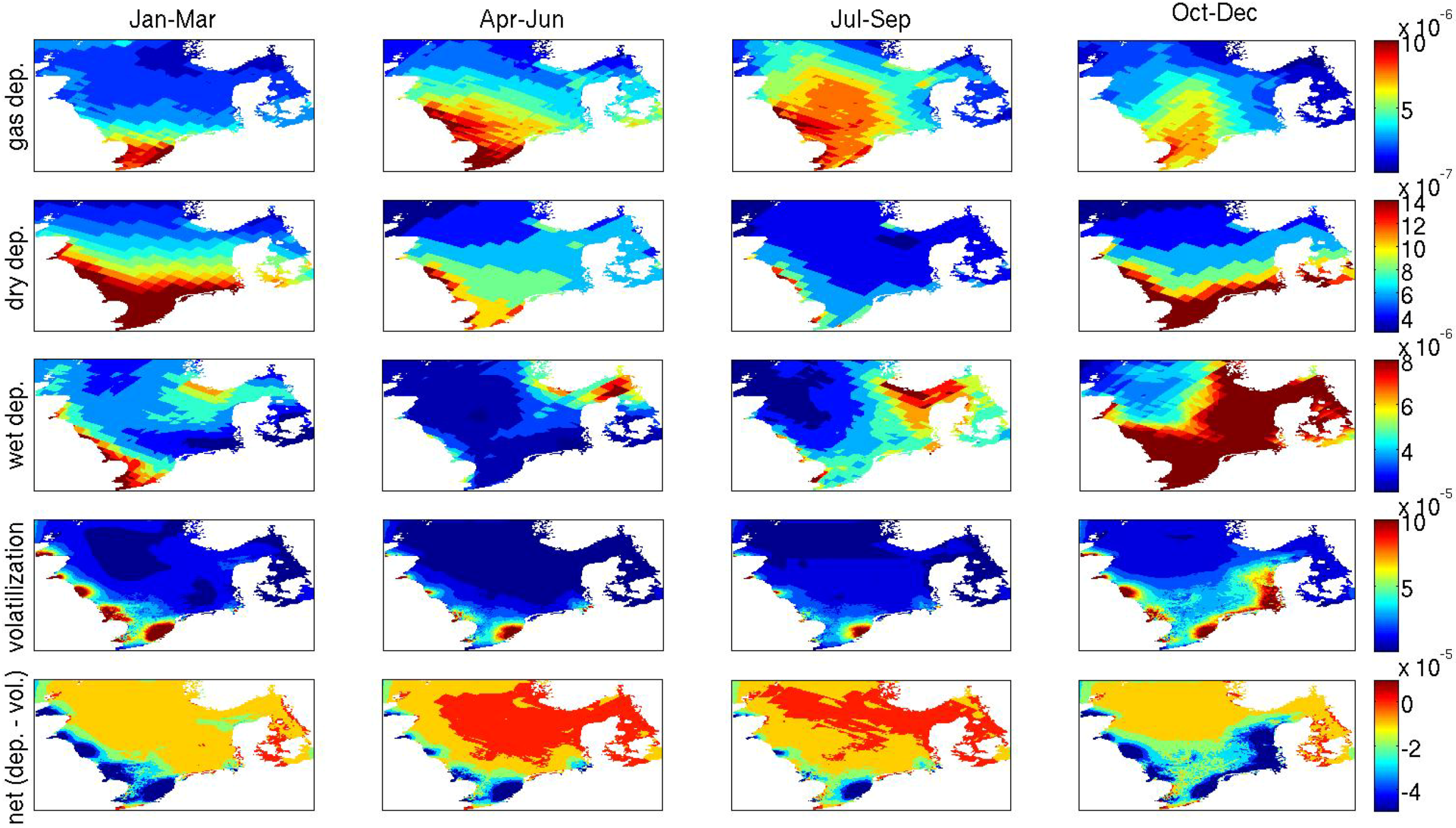
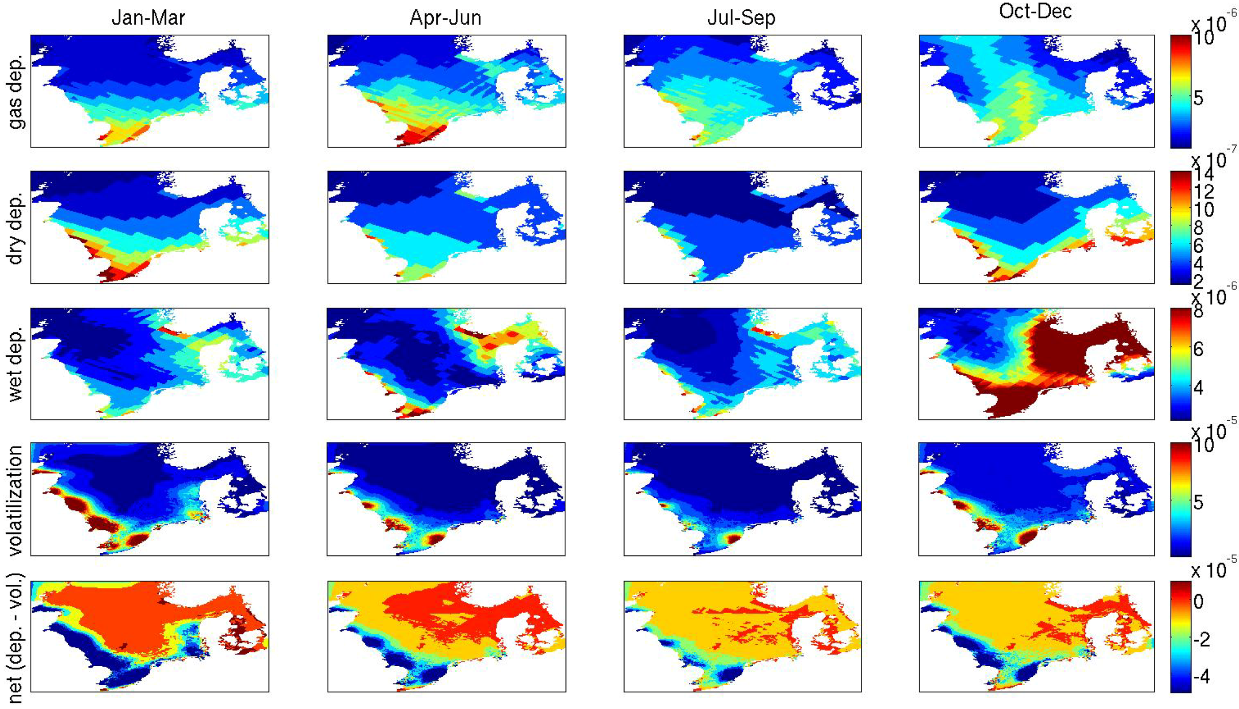
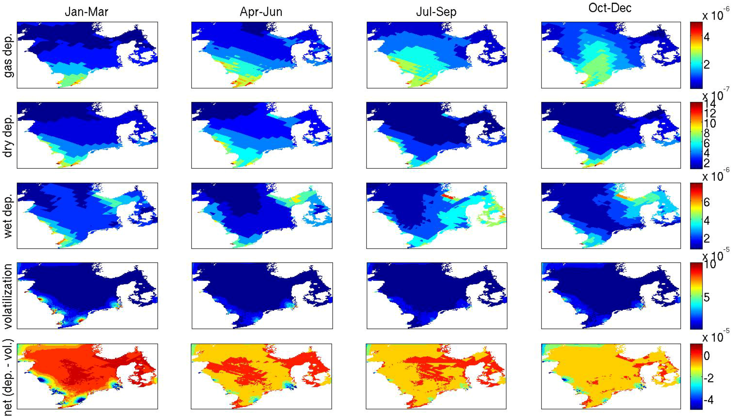
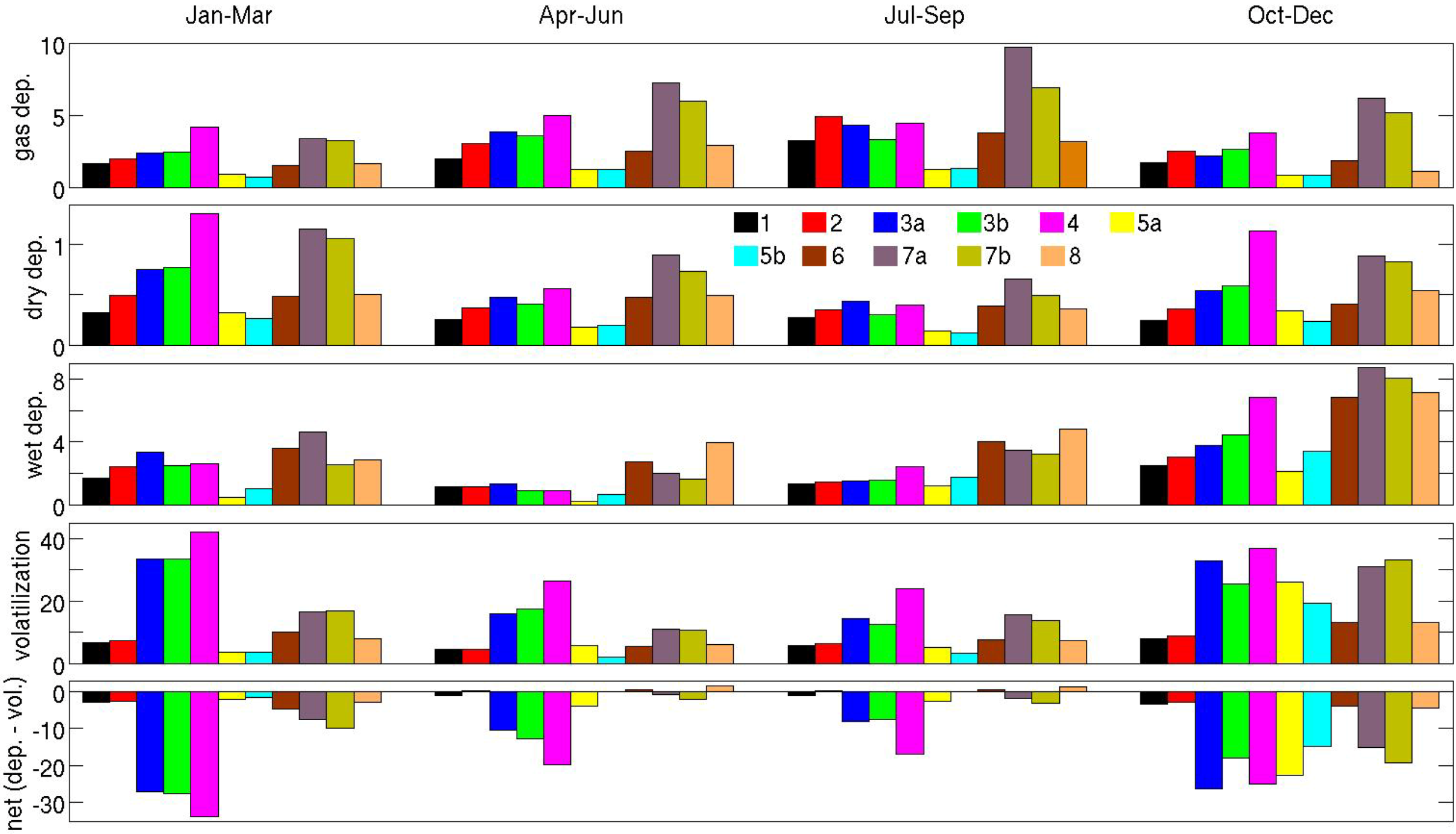
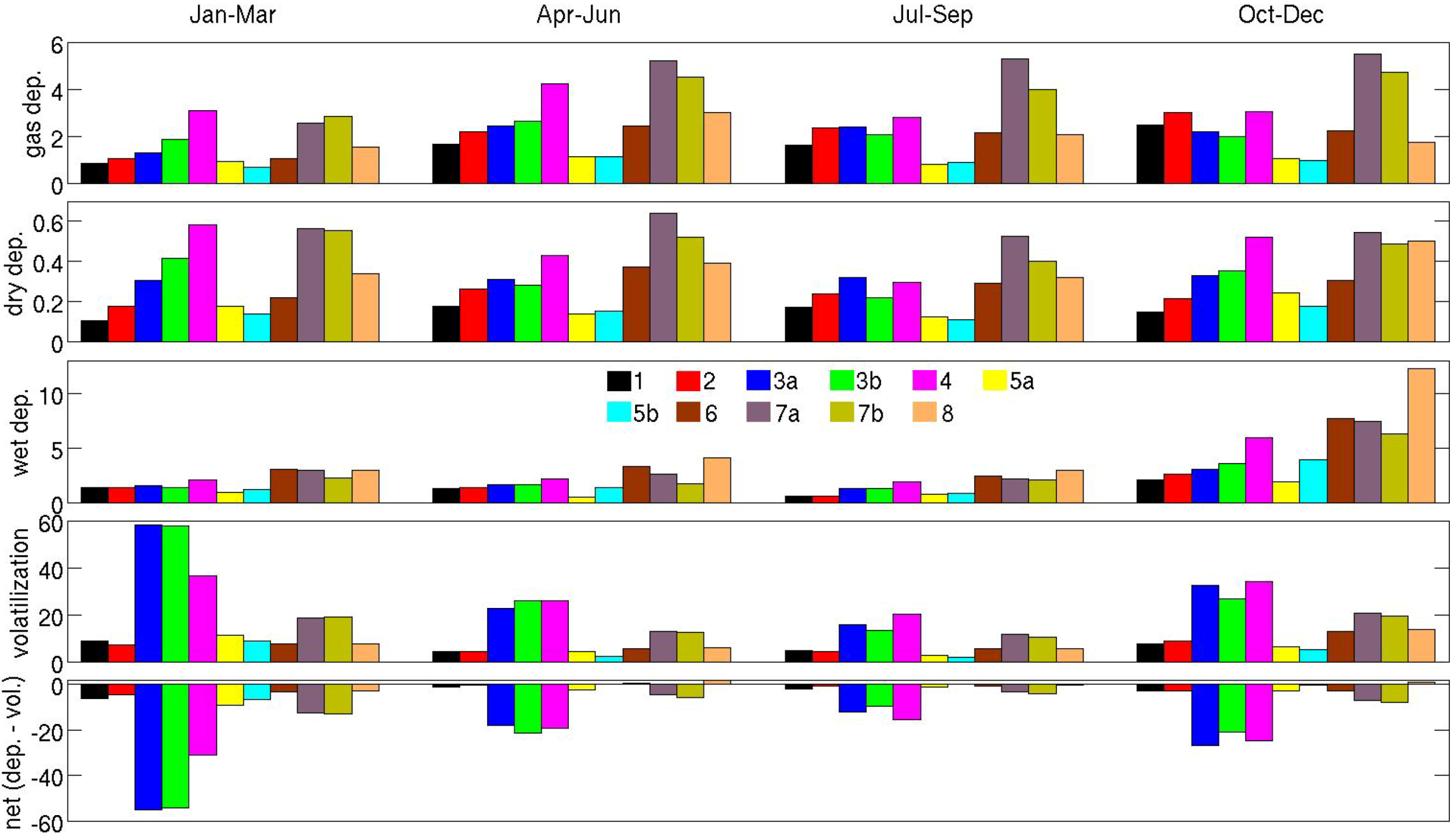
3. Results and Discussion
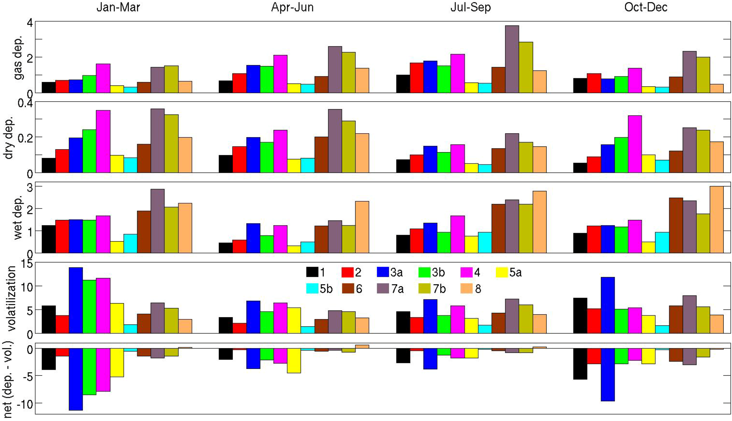
3.1. Gas Deposition


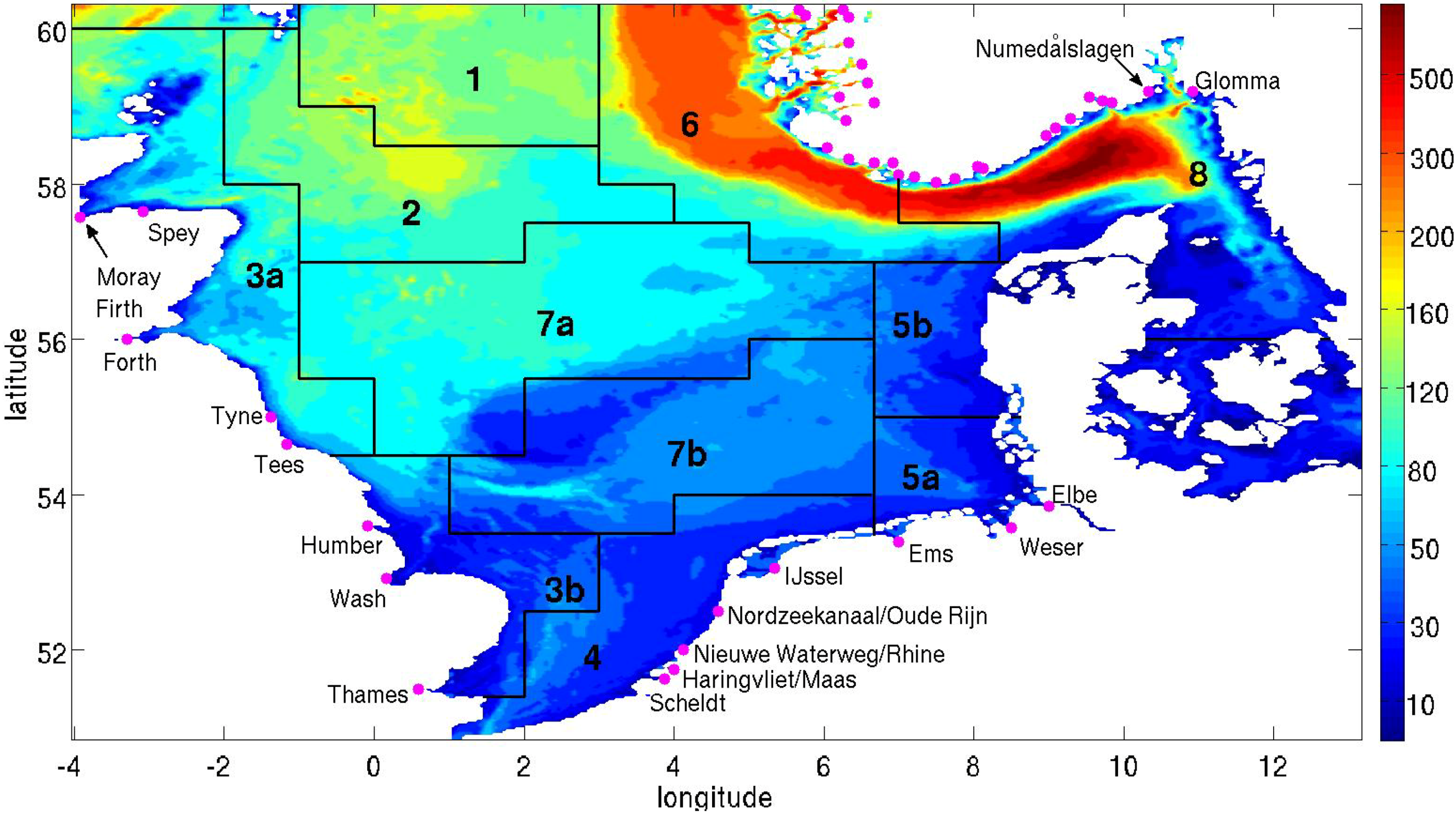
| Box Number | 1 | 2 | 3a | 3 | 4 | 5a | 5b | 6 | 7a | 7b | 8 |
| Area (km2) | 23,566 | 29,995 | 31,404 | 16,113 | 25,314 | 10,415 | 11,855 | 32,885 | 52,554 | 37,943 | 31,961 |
3.1.2. PCB 153


3.2. Dry Deposition
3.2.2. PCB 153
3.3. Wet Deposition
3.3.2. PCB 153
3.4. Volatilization
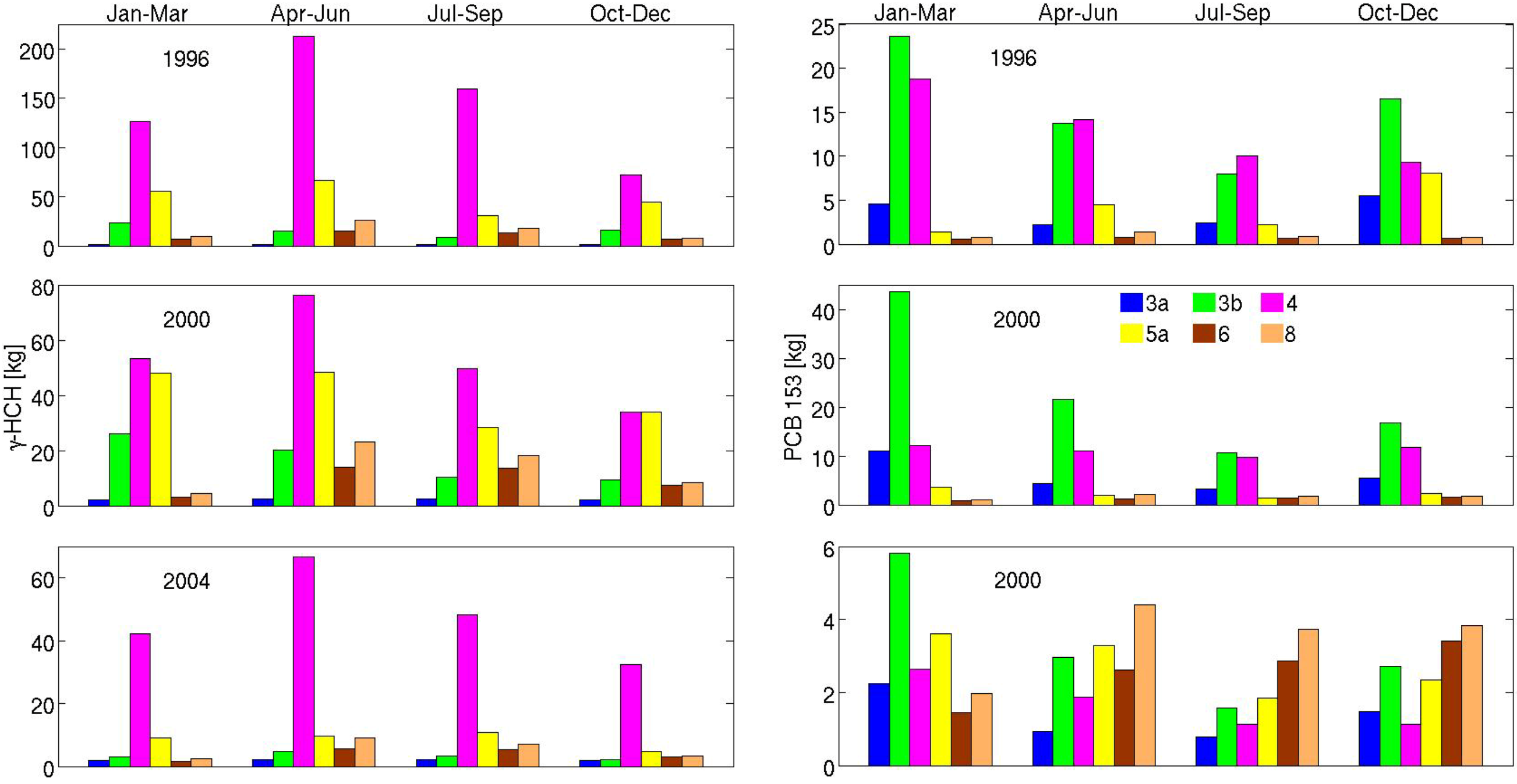
3.4.1. γ-HCH
3.4.2. PCB 153

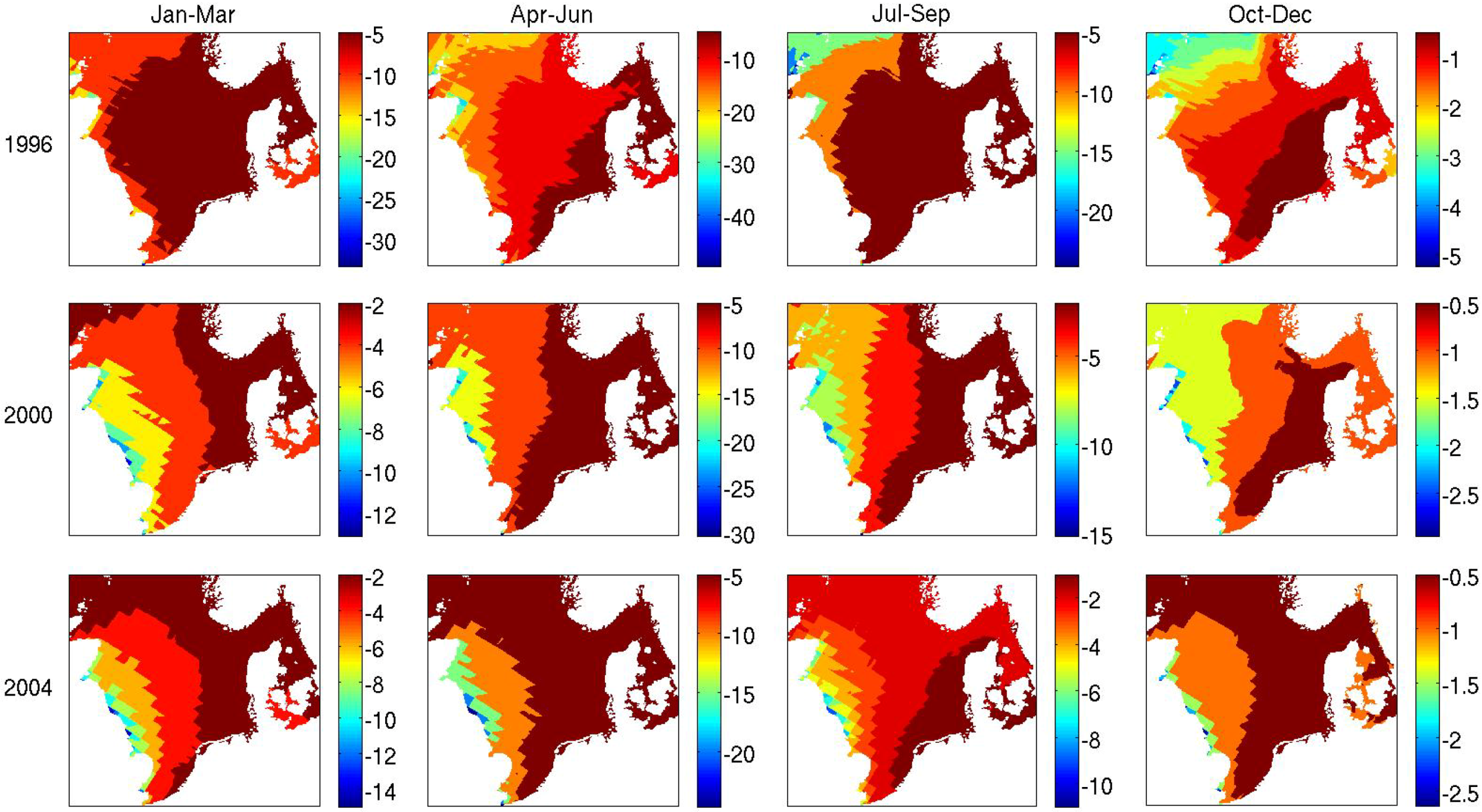
3.5. Net Air-Sea Exchange and Fugacity Ratios
3.5.1. γ-HCH
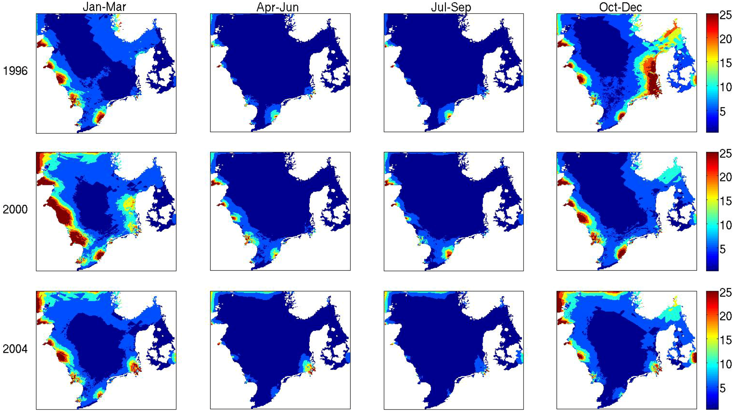
3.5.2. PCB 153

4. Summary and Conclusions
Acknowledgments
Conflicts of Interest
References
- Gioia, R.; Nizzetto, L.; Lohmann, R.; Dachs, J. Polychlorinated biphenyls (PCBs) in air and seawater of the Atlantic Ocean: Sources, trends and processes. Environ. Sci. Tech. 2008, 42, 1416–1422. [Google Scholar] [CrossRef]
- Nizzetto, L.; Lohmann, R.; Gioia, R.; Dachs, J.; Jones, K.C. Atlantic Ocean surface waters buffer declining atmospheric concentrations of persistent organic pollutants. Environ. Sci. Tech. 2010, 44, 6978–6984. [Google Scholar] [CrossRef]
- Guglielmo, F.; Lammel, G.; Maier-Reimer, E. Global environmental cycling of γHCH and DDT in the 1980s: A study using a coupled atmosphere and ocean general circulation model. Chemosphere 2009, 76, 1509–1517. [Google Scholar] [CrossRef]
- Ilyina, T.; Lammel, G.; Pohlmann, T. Mass budgets and contribution of individual sources and sinks to the abundance of gamma-HCH, alpha-HCH and PCB 153 in the North Sea. Chemosphere 2008, 72, 1132–1137. [Google Scholar] [CrossRef]
- Gusev, A.; Rozovskaya, O.; Shatalov, V.; Sokovyh, V.; Aas, W.; Breivik, K. Persistent Organic Pollutants in the Environment; Status Report 3; EMEP Meteorological Synthesizing Centre-East: Moscow, Russia, 2009. [Google Scholar]
- Lenhart, H.-J.; Pohlmann, T. The ICES-boxes approach in relation to results of a North Sea circulation model. Tellus 1997, 49, 139–160. [Google Scholar]
- Luff, R.; Pohlmann, T. Calculation of water exchange times in the ICES-boxes with a eulerian dispersion model using a half-life time approach. Deut. Hydrogr. Z. 1996, 47, 287–299. [Google Scholar] [CrossRef]
- O’Driscoll, K.; Mayer, B.; Ilyina, T.; Pohlmann, T. Modelling the cycling of persistent organic pollutants (POPs) in the North Sea system: Fluxes, loading, seasonality, trends. J. Mar. Syst. 2013, 111/112, 69–82. [Google Scholar] [CrossRef]
- Ilyina, T.; Pohlmann, T.; Lammel, G.; Sündermann, J. A fate and transport ocean model for persistent organic pollutants and its application to the North Sea. J. Mar. Syst. 2006, 63, 1–19. [Google Scholar] [CrossRef]
- Backhaus, J. A three-dimensional model for the simulation of shelf sea dynamics. Deut. Hydrogr. Z. 1985, 38, 165–187. [Google Scholar] [CrossRef]
- Pohlmann, T. A meso-scale model of the central and southern North Sea: Consequences of an improved resolution. Cont. Shelf Res. 2006, 26, 2367–2385. [Google Scholar] [CrossRef]
- Larsen, J.; She, J. Optimisation of a Bathymetry Database for the North European Shelf Seas; Technical Report 01–21; Danish Meteorological Institute: Copenhagen, Denmark, 2001.
- Kalnay, E.; Kanamitsu, M.; Kistler, R.; Collins, W.; Deaven, D.; Gandin, L.; Iredell, M.; Saha, S.; White, G.; Woollen, J.; et al. The NCEP/NCAR 40-year reanalysis project. Bull. Am. Meteorol. Soc. 1996, 77, 437–471. [Google Scholar] [CrossRef]
- Kistler, R.; Kalnay, E.; Collins, W.; Saha, S.; White, G.; Woollen, J.; Chelliah, M.; Ebisuzaki, W.; Kanamitsu, M.; Kousky, V.; et al. The NCEP/NCAR 50-year reanalysis: Monthly means CD-ROM and documentation. Bull. Am. Meteorol. Soc. 2001, 82, 247–267. [Google Scholar] [CrossRef]
- Orlanski, I. A simple boundary condition for unbounded hyperbolic flows. J. Comput. Phys. 1976, 21, 251–269. [Google Scholar] [CrossRef]
- Boyer, T.; Levitus, S.; Garcia, H.; Locarnini, R.; Stephens, C.; Antonov, J. Objective analyses of annual, seasonal, and monthly temperature and salinity for the world ocean on a 0.25° grid. Int. J. Climatol. 2005, 25, 931–945. [Google Scholar] [CrossRef]
- Smagorinsky, J. General circulation experiments with the primitive equations. I. The basic experiment. Mon. Weather Rev. 1963, 91, 99–164. [Google Scholar]
- Kochergin, V.P. Three-Dimensional PrognosticModels. In Coastal and Estuarine Science; American Geophysical Union: Washington, DC, USA, 1987. [Google Scholar]
- Damm, P.E. Die Saisonale Salzgehalts- und Frischwasserverteilung in der Nordsee und ihre Bilanzierung; Institut für Meereskunde: Hamburg, Germany, 1997. [Google Scholar]
- Lewin, J.; Weir, M.J.C. Morphology and recent history of the Lower Spey. Scott. Geogr. J. 1977, 93, 45–51. [Google Scholar]
- Whitman, W.G. The two-film theory of gas absorption. Chem. Metall. Eng. 1923, 29, 146–150. [Google Scholar]
- Liss, P.S.; Slater, P.G. Flux of gases across the air–sea interface. Nature 1977, 247, 181–184. [Google Scholar] [CrossRef]
- Mackay, D. Multimedia Environmental Models: The Fugacity Approach, 2nd ed.; Lewis: Boca Raton, FL, USA, 2001. [Google Scholar]
- Wania, F.; Persson, J.; di Guardo, A.; McLachlan, M. The Popcycling-Baltic Model.A Non-steady State Multicompartment Mass Balance Model of the Fate of Persistent Organic Pollutants in the Baltic Sea Environment; Tech. Rep. OR 10/2000; U-96069; Norwegian Institution Air Research: Kjeller, Norway, 2003. [Google Scholar]
- Schwarzenbach, R.E.; Gschwend, P.M.; Imboden, D.M. Environmental Organic Chemistry, 1st ed.; Wiley: New York, NY, USA, 1993. [Google Scholar]
- Malanichev, A.; Mantseva, E.; Shatalov, V.; Strukov, B.; Vulykh, N. Numerical evaluation of the PCB transport over the northern hemisphere. Environ. Pollut. 2004, 128, 279–289. [Google Scholar] [CrossRef]
- Wodarg, D.; Kömp, P.; McLachlan, M.S. A baseline study of polychlorinated biphenyl and hexachlorobenzene concentrations in the western Baltic Sea and Baltic proper. Mar. Chem. 2003, 87, 23–36. [Google Scholar] [CrossRef]
- Schulz-Bull, D.E.; Petrick, G.; Bruhn, R.; Duinker, J.C. Chlorobiphenyls (PCB) and PAHS in water masses of the northern North Atlantic. Mar. Chem. 1998, 61, 101–114. [Google Scholar] [CrossRef]
- Schulz-Bull, D.E.; Hand, I.; Lerz, A.; Trost, E.; Wodarg, D. Regionale Verteilung Chlorierter Kohlenwasserstoffe (CKW) und Polycyclischer aromatischer Kohlenwasserstoffe (PAK) im Pelagial und Oberflchensediment der Ostsee 2008; Auftrag des Bundesamtes fürSeeschifffahrt und Hydrographie; Leibniz-Institut für Ostseeforschung an der Universität Rostock: Rostock, Germany; p. 2009.
- Iwata, H.; Tanabe, S.; Sakai, N.; Tatsukawa, R. Distribution of persistent organochlorines in the oceanic air and surface seawater and the role of ocean on their global transport and fate. Environ. Sci. Tech. 1993, 27, 1080–1098. [Google Scholar] [CrossRef]
- Lakaschus, S.; Weber, K.; Wania, F.; Bruhn, R.; Schrems, O. The air-sea equilibrium and time trend of hexachlorocyclohexanes in the Atlantic ocean between the Arctic and Antarctica. Environ. Sci. Tech. 2002, 36, 138–145. [Google Scholar] [CrossRef]
- Lorkowski, I.; Pätsch, J.; Moll, A.; Kühn, W. Interannual variability of carbon fluxes in the North Sea (1970–2006)—Abiotic and biotic drivers of the gas-exchange of CO2. Estuar. Coast. Shelf Sci. 2012, 100, 38–57. [Google Scholar] [CrossRef]
- Shatalov, V.; Dutchak, S.; Fedyunin, M.; Mantseva, E.; Strukov, B.; Varygina, M.; Vulykh, N.; Aas, W.; Mano, S. Persistent Organic Pollutants in the Environment; Status Report 3; EMEP Meteorological Synthesizing Centre-East: Moscow, Russia, 2003. [Google Scholar]
- Gusev, A.; Mantseva, E.; Rozovskaya, O.; Shatalov, V.; Vulykh, N.; Aas, W.; Breivik, K. Persistent Organic Pollutants in the Environment; Status Report 3; EMEP Meteorological Synthesizing Centre-East: Moscow, Russia, 2006. [Google Scholar]
- OSPAR Commission. Quality Status Report 2000, Region II—Greater North Sea; OSPAR Commission: London, UK, 2000. [Google Scholar]
- Bruhn, R.; Lakaschus, S.; McLachlan, M.S. Air/sea gas exchange of PCBs in the southern Baltic Sea. Atmos. Environ. 2003, 37, 3445–3454. [Google Scholar] [CrossRef]
- Sundqvist, K.L.; Wingfors, H.; Brorstöm-Lundén, E.; Wiberg, K. Air-sea gas exchange of HCHs and PCBs and enantiomers of α-HCH in the Kattegat Sea region. Environ. Pollut. 2004, 128, 73–83. [Google Scholar] [CrossRef]
- Harner, T.; Bidleman, T.F.; Jantunen, L.M.M.; Mackay, D. Soil-air exchange model of persistent pesticides in the US Cotton Belt. Environ. Toxicol. Chem. 2001, 20, 1612–1621. [Google Scholar]
- Palm, A.; Cousins, I.; Gustafsson, Ö.; Axelman, J.; Grunder, K.; Broman, D.; Brorstöm-Lundén , E. Evaluation of sequentially-coupled POP fluxes estimated from simultaneous measurements in multiple compartments of an air-water-sediment system. Environ. Pollut. 2004, 128, 85–97. [Google Scholar] [CrossRef]
© 2014 by the authors; licensee MDPI, Basel, Switzerland. This article is an open access article distributed under the terms and conditions of the Creative Commons Attribution license (http://creativecommons.org/licenses/by/3.0/).
Share and Cite
O'Driscoll, K. Air-Sea Exchange of Legacy POPs in the North Sea Based on Results of Fate and Transport, and Shelf-Sea Hydrodynamic Ocean Models. Atmosphere 2014, 5, 156-177. https://doi.org/10.3390/atmos5020156
O'Driscoll K. Air-Sea Exchange of Legacy POPs in the North Sea Based on Results of Fate and Transport, and Shelf-Sea Hydrodynamic Ocean Models. Atmosphere. 2014; 5(2):156-177. https://doi.org/10.3390/atmos5020156
Chicago/Turabian StyleO'Driscoll, Kieran. 2014. "Air-Sea Exchange of Legacy POPs in the North Sea Based on Results of Fate and Transport, and Shelf-Sea Hydrodynamic Ocean Models" Atmosphere 5, no. 2: 156-177. https://doi.org/10.3390/atmos5020156