Local Climate Classification and Dublin’s Urban Heat Island

Abstract

A recent re-evaluation of urban heat island (UHI) studies has suggested that the urban effect may be expressed more meaningfully as a difference between Local Climate Zones (LCZ), defined as areas with characteristic dimensions of between one and several kilometers that have distinct effects on climate at both micro-and local-scales (city streets to neighborhoods), rather than adopting the traditional method of comparing urban and rural air temperatures. This paper reports on a UHI study in Dublin (Ireland) which maps the urban area into LCZ and uses these as a basis for carrying out a UHI study. The LCZ map for Dublin is derived using a widely available land use/cover map as a basis. A small network of in-situ stations is deployed into different LCZ across Dublin and additional mobile temperature traverses carried out to examine the thermal characteristics of LCZ following mixed weather during a 1 week period in August 2010. The results show LCZ with high impervious/building coverage were on average >4 °C warmer at night than LCZ with high pervious/vegetated coverage during conditions conducive to strong UHI development. The distinction in mean LCZ nocturnal temperature allows for the generation of a heat map across the entire urban area.

1. Introduction

Cities represent the most significant human environments, both in terms of the physical artefacts and socio-economic activities associated with the processes of urbanization. The introduction of complex geometries that comprise cities onto the natural landscape has long been known to dramatically alter the surface energy balance at the interface of the surface and the atmosphere i.e., the planetary boundary layer. The physical presence of cities alters the radiative, aerodynamic, thermal and moisture properties of the atmosphere in and around urban areas. The most pronounced effect detectable is that of positive thermal anomalies associated with nocturnal urban air temperature. This urban heat island (UHI) effect broadly speaking is a reflection of the totality of micro-climatic changes instigated by urbanization. Much recent work on the UHI has shown this anomaly can be detected at multiple temporal and spatial scales; the warming signal, its causes and implications, are dependent on the scale of investigation, from individual buildings over hours to encompassing entire urban areas over years. However, the most commonly studied UHI is the near-surface air temperature found below roof level within the urban canopy layer (UCL) [1]. As this is where humans live and work the magnitude of the UHI is directly relevant to studies of human health and comfort and building energy management.

There is a considerable body of literature on this UHI, which extends back to the work of Luke Howard in London at the beginning of the 19th Century [2] and it remains a topic of current research in different cities and climates; see for example recent studies in North America [3,4,5], Asia [6] and Europe [7,8]. Typical UHI measurement studies have taken two approaches: make temperature observations at conventional stations located in urban and rural environments, and measure temperature along a transect from the rural environment to the city center using a mobile platform. Critically, both approaches evaluate the UHI by comparing urban (U) observations with rural (R) or background temperatures (ΔT_U-R). A near universal finding is that the intensity of a UHI (the magnitude of ΔT_U-R) at a given place is greatest at night when the synoptic conditions can be characterized by high pressure, clear skies, little wind and no precipitation. Other factors, such as the contribution of anthropogenic heat (as a result of traffic or heating/cooling systems) or changes in vegetative cover during the year will modulate the strength of the UHI during the year. The urban structure itself (the materials, the buildings and their layout) also regulates the magnitude of the temperature effect across the city producing the classic island form with values increasing from the edge to the city center.

The causes for UHI are best understood in terms of the energy budget (Oke [9]):

Q* + Q_F =Q_H +Q_E +ΔQ_S +ΔQ_A W∙m⁻²

(1)

This describes the energy exchanges across the sides of a notional “box” that extends to a level above the surface and to a depth in the substrate affected by the diurnal thermal regime. It states that net radiation (Q*) is partitioned into the turbulent fluxes of sensible (Q_H) and latent (Q_E) heat and energy storage (ΔQ_S). The advective term (ΔQ_A), which describes horizontal transfers through the sides across the box is generally ignored unless the study site straddles two very different urban landscapes (such as a park boundary, for example). Finally, the anthropogenic heat flux (Q_F) is energy added by human activities. The net radiation term can be further decomposed into incoming (↓) and outgoing (↑) shortwave (K) and longwave (L) radiation terms:

Q* = (K↓ − K↑) + (L↓ − L↑) or Q* = K* +L*

(2)

The magnitudes of these terms will vary with the microclimatic environment. To generalize the typical UCL setting, Oke [9,10] considered how these terms would be affected in a typical city street, or urban canyon. For instance the trapping and additional reflection of radiation [11,12] the addition of anthropogenic energy into the balance and its subsequent channeling into the turbulent fluxes [13,14,15] as well as surface thermal properties themselves [16,17,18] which are unique to urban areas verses their rural counterparts (Table 1).

Table 1. Connection between energy budget/urban heat island (UHI) within the canopy-layer. Modified from [9,10].

Energy Balance Term (Relative to Rural Areas)	Urban Feature within UCL (LCZ)	Urban Effect	Selected Study on Specific Feature
Increased K*	Canyon Geometry	Increased surface area and trapping of radiation	[11,12]
Increased L↓	Air Pollution	Greater absorption and re-emission	[11,12]
Decreased L*	Canyon Geometry	Reduced Sky View Factor (less nocturnal loss)	[12]
Addition of QF	Buildings and Traffic	Direct addition of heat	[13,14,15]
Increased ∆QS	Construction Materials	Increased thermal admittance	[16,17]
Decreased QE	Construction Materials	Increased water-proofing	[17,18]
Decreased QA	Canyon Geometry	Reduces wind speed	[11]

Table 1. Connection between energy budget/urban heat island (UHI) within the canopy-layer. Modified from [9,10].

Energy Balance Term (Relative to Rural Areas)	Urban Feature within UCL (LCZ)	Urban Effect	Selected Study on Specific Feature
Increased K*	Canyon Geometry	Increased surface area and trapping of radiation	[11,12]
Increased L↓	Air Pollution	Greater absorption and re-emission	[11,12]
Decreased L*	Canyon Geometry	Reduced Sky View Factor (less nocturnal loss)	[12]
Addition of QF	Buildings and Traffic	Direct addition of heat	[13,14,15]
Increased ∆QS	Construction Materials	Increased thermal admittance	[16,17]
Decreased QE	Construction Materials	Increased water-proofing	[17,18]
Decreased QA	Canyon Geometry	Reduces wind speed	[11]

During ideal UHI conditions (night-time (K* = 0), calm (Q_H + Q_E ≈ 0) and clear skies) long-wave radiation loss is compensated for by the withdrawal heat from storage and the anthropogenic heat flux; hence, the distinction between urban and non-urban environments then is due to the rate of night-time cooling [2]. The evidence shows that the air temperature in a densely-built UCL cools nearly linearly after sunset while that in the non-urban setting cools exponentially [9]; hence, ΔT_U-R is greatest about 4 h after sunset. It follows then that near-surface air temperature and its variation over space and time is an integral measure of changes in the microclimatic conditions (and energy budgets). However, until recently there has been little consideration of the character of the urban surface (and of the rural surface) that produces distinctive ΔT_U-R values. Despite the vast amount of intellectual investment on the UHI, the field has lacked a unified (i.e., international) method of investigating and reporting on the UHI [19,20]; hence, there is little expression of universality between studies on the UHI save for their topic of investigation. This has made the comparison of individual studies across different cities difficult.

Stewart and Oke [20] have provided a much needed context for UHI studies by categorizing the myriad of microclimatic environments into distinctive neighborhood-scale (≥1 km²) types known as Local Climate Zones (LCZ). This scheme incorporates the four properties of the urban environment that contribute to the UHI, namely: fabric (construction and natural materials); cover (built-up, paved, vegetated, bare soil, water); structure (dimensions of the buildings and the spaces between them, the street widths and street spacing) and; metabolism (heat, water and pollutants due to human activity) [20]. The basic classification system consists of 10 urban zones and seven non-urban zone types that represent a universal nomenclature; a supplement to [19] provides detailed datasheets on each LCZ type that includes photographs and parameter values that typify each zone. Hence, rather than measuring the UHI in terms of naively classified “urban” and “rural” settings (i.e., ΔT_U-R), the LCZ scheme offers the potential for observing and communicating the urban temperature effect in terms of differences between neighborhoods that incorporate the microclimatic process that is responsible (ΔT_LCZ). The LCZ scheme has already been used in a few studies to describe parts of the urban landscape [21,22] principally to map thermal source areas of screen-height thermal sensors as was the intended application of LCZ. Currently, there is no “systematic” means of mapping an entire city into LCZ types; instead the researcher uses the LCZ datasheets in conjunction with fieldwork, aerial images and existing urban databases to decide on the extent of a neighborhood and its type.

This paper reports on a UHI study in Dublin, Ireland conducted during the summer 2010, which used the LCZ system to structure the observations and interpret the results. While Dublin’s UHI has been examined before, these studies have used conventional approaches. Here, we test a number of propositions:

(i)

The urban area can be decomposed into LCZ types using widely available data;

(ii)

The LCZ map is a useful first step for structuring a UHI study and;

(iii)

The LCZ type provides a physically-based context for explaining near-surface air temperature variations over space.

Here, the LCZ map is used to position a small network of identical meteorological stations (using the recommendations given by [9,23]) and to devise a mobile traverse route to sample night-time air temperatures across the city.

2. Methodology

2.1. Study Area

Dublin (53.5°N, 6.5°W) is the capital of the Republic of Ireland and is one of the most westerly cities in Europe (see Figure 1). The city is located on the east coast and is flanked by the Irish Sea to the East, and the Dublin/Wicklow mountains to the South. With the exception of the mountainous southern part, most of the city occupies a flat and low-lowing basin (<100 m a.s.l.) and is bisected by the Liffey River. It occupies a maritime-temperature climate (Köppen Cfb) and the relevant monthly averages (and ranges) for the climatological period 1980–2010 are as follows: air temperature is 10 (±5) °C; wind speed 5.3 (±1) m∙s⁻¹; precipitation 63 (±10) mm; days with ≥0.2 mm of rain 16 (±1) and; daily sunshine hours 4 (±2) [24]. Given its latitude, it has a mild climate with little temperature variation through the year although day-length is significant longer in summer (16 h in June) than in winter (8 h in December). The extent of the urban area under investigation extends to ~700 km² as the city has expanded outside its administrative boundaries over the last three decades. The population of the defined urban area is about 1.2 million [25].

Owing to its generally wet and windy climate, the average UHI in Dublin is small in magnitude; strong and persistent anticylonic conditions that are conducive to strong UHI formation occur infrequently. The few UHI studies that have been completed have been undertaken during these ideal conditions (i.e., calm and clear conditions, after sunset and following a dry period). Moreover, in the absence of a network of stations, traverse methods have been used. Sweeney [26] conducted mobile temperature traverses across the city during winter, reporting that UHI magnitude (ΔT_U-R) could reach 6.5 °C in settled anticyclonic conditions approximately 4 h after local sunset. Graham [27] adopted a similar approach, conducting mobile temperature traverses during the summer months both day and night, and reported a UHI intensity of approximately 4.5 °C during the night, again approximately 4 h after local sunset. Both studies alluded to but ultimately neglected the impact of building density and form on the spatial character of the UHI. The role of wider synoptic conditions specifically the movement of mid-latitude cyclones over the city was shown to either mitigate (in cyclonic situations) or enhance (in anticyclonic situations) development of the nocturnal UHI. Temperature gradients were diminished in wind speeds over 7 m∙s⁻¹.

Figure 1. Study Area of Dublin City, Capital of the Republic of Ireland.

Figure 1. Study Area of Dublin City, Capital of the Republic of Ireland.

2.2. Study Design

To conduct this UHI study we took the following steps:

(i)

Mapped the study area into Local Climate Zone types (Section 2.3)

(ii)

Devised an observational campaign to explore Dublin’s UHI under ideal conditions using the LCZ map. This included:

(a)

Positioning six identical weather stations across the study area (Section 2.4/Table 2)

(b)

Planning traverse routes through specific LCZ types (Section 2.4)

(iii)

Analyzed air temperature observations in the context of LCZ type, that is, derive T_LCZ (Section 2.5)

2.3. Mapping the Study Area

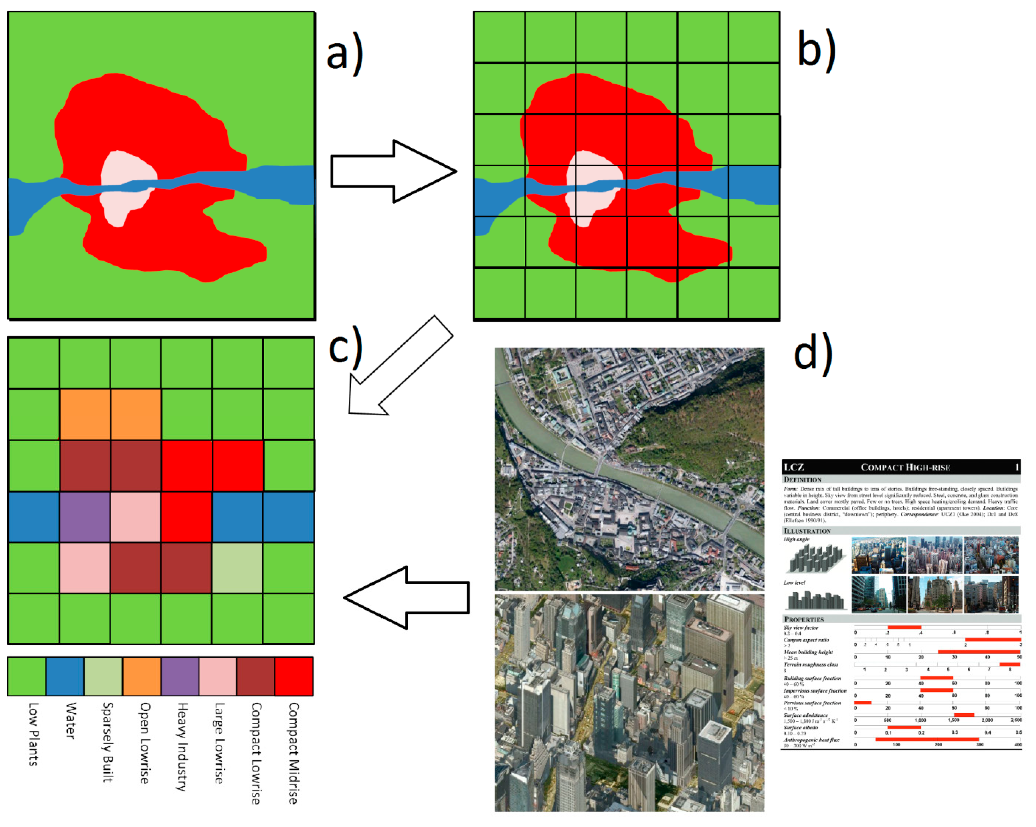
Concluding from the summarized literature, there is a need to standardize the method for decomposing the urban area into LCZ. Ideally, detailed spatial data on urban structure, cover, fabric and metabolism would be available, as was used in Unger et al. [28] for the purpose but this is rarely the case. An alternative approach using multi-temporal remotely sensed data from the Landsat platform has been tested by Bechtel [29] and Bechtel and Daneke [30] but this process is still in development. As an alternative to both methods and sensitive to the lack of detailed morphological data for our study area, here we employ the LULC dataset Corine, developed by the European Environment Agency to satisfy a number of user needs. Its uses a minimum mapping unit of 25 hectares (0.25 km²) and employs 44 land cover classes [31]. Of particular relevance here is translating the categories for Artificial (urban) surfaces, which include the following: continuous urban fabric; discontinuous urban fabric; industrial or commercial units and transport units. It also has subcategories under Agricultural, Forests & Semi-Natural, and Wetland area categories. This dataset is suited for our purposes subject to changing the spatial resolution and “translating” from the LULC category into an LCZ type. While Corine provides data at a high spatial resolution, the myriad of differences in built form leads to high spatial variability. However, as the spatial scale is increased, there is likely to be a corresponding reduction in spatial variability [32] meaning that at the local scale (>500 m) LCZ types should exhibit a unique thermal climate. A grid-based sampling approach was employed to generate our LCZ map. This was selected as it was deemed to be the simplest means by which to resample irregularly spaced data into a regular grid thus provide a systematic means to subsequently examine aerial and oblique images, plan traverse routes and deploy our network of stations. The use of the grid approach also introduces some level of objectivity to the process of generating the LCZ map given that each grid is coded based on the majority of LULC pixels it contains. The major disadvantage of this approach is a loss of detail in parts of the city where the urban landscape is fragmented into small areas and at border areas, but for most of the study area this process simply decomposes very large areas (>1 km²) into smaller spatial units. Our selected grid size is 1 km², which corresponds to the local or neighborhood-scale for which the LCZ scheme was designed.

When each grid was coded with a LULC category a number was randomly selected for examination to provide a link to LCZ type. Google-Earth (GE) and BingMaps (BM) were used to translate each selected grid cell LULC into a corresponding LCZ class using the LCZ datasheets [19]. Both GE and BM are freely available web-based tools and provide detailed oblique aerial images, similar to those used as exemplars by the LCZ datasheets. In most cases, the link between LULC and LCZ class was clear based on expert judgment. Where there was some difficulty, field-work was used to help in making the decision. Figure 2 depicts the procedure. Once complete the LULC grid values were converted into LZC types for the next step.

2.4. Observation Campaign

The examination of Dublin’s UHI under ideal conditions was designed within the context of the LCZ. Our approach was based on measurements made at fixed stations supplemented by traverses using mobile stations. Six meteorological stations were positioned so as to represent the variety of LCZ types across the city, which occupy different sized areas. These stations consisted of a complete automated identical integrated sensor suite (Davis Vantage Vue^©) housed in UV-resistant ABS & ASA plastic (reported accuracy in parenthesis), each of which has a shielded thermo-hydro sensors (±0.5 °C, ±3%), an anemometer (±1 m∙s⁻¹), a wind-vane (±3°) and a rain-gauge (±0.2 mm). These instruments were interrogated at 30 min intervals and were naturally ventilated.

Figure 2. Summary of Local Climate Zone (LCZ) classification procedure (a) Hypothetical LULC map for area (b) a neighborhood scale (~1 km) grid imposed (c) grids and LULC used as a basis for field work and visual inspection of open source imagery, each area classified into LCZ most representative (d) example of Quick-Bird (Google-Earth) and Birds-eye image (Microsoft BingMaps) and LCZ classification sheet (reproduced from [19]).

Figure 2. Summary of Local Climate Zone (LCZ) classification procedure (a) Hypothetical LULC map for area (b) a neighborhood scale (~1 km) grid imposed (c) grids and LULC used as a basis for field work and visual inspection of open source imagery, each area classified into LCZ most representative (d) example of Quick-Bird (Google-Earth) and Birds-eye image (Microsoft BingMaps) and LCZ classification sheet (reproduced from [19]).

Positioning meteorological stations in urban areas is a challenging task that is recognized in WMO guidelines [33]. For air temperature observations, the suggested exposure should be representative of the urban climate zone (LCZ) and with a distance greater than 1 m from walls. Particular attention should be given to radiation shields and ventilation, owing to the shading and sheltering effects of buildings. On the other hand, the guidelines provide for considerable leeway in terms of height as the UCL is well mixed such that measurements up to 5 m are little different from those obtained at standard height. Here, each station was positioned well within a LCZ type at a location that we considered to be both secure and representative of that LCZ. The station itself was affixed to available structures at different heights but always within the UCL; we took care to ensure that each station was exposed to natural airflow and was not excessively sheltered by obstacles. The guidelines suggest that the “circle of influence” for the temperature sensor will have a radius of 500 m typically but this is likely to depend on the character of the surrounding urban area and boundary-layer conditions [33,34,35]. Table 2 shows the location of each station in relation to the surrounding landscape and LCZ type; their location with the study region is shown in Figure 3.

Table 2. Metadata descriptions accompanying the six fixed weather stations used in this study. The columns represent the LCZ type, description of the site location and an aerial image (the circle shows the location of the station). In the description column, all heights are in meters above the ground (AG) and above sea-level (ASL). Corresponding LCZ images (first column) are reproduced from [19].

LCZ	Station Description		Aerial View (Extent ~ 500 × 500 m)
Low Plants Located off grounds of laboratory run by national agriculture research institute	Station 1—North East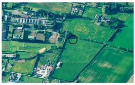
	Station AG Height	1.9
	Station ASL Height	3.6
	Average Building Height	6.5
	Surface below sensor	Grass
	Dominant Surface around site	Grass/Roads
Compact Lowrise Located on grounds of school	Station 2—South East
	Station AG Height	3.7
	Station ASL Height	47
	Average Building Height	7.0
	Surface below sensor	Pavement
	Dominant Surface around site	Pave/Buldings
Open Midrise Located on grounds of university	Station 3—South Central
	Station AG Height	3.7
	Station ASL Height	22
	Average Building Height	14.5
	Surface below sensor	Grass/Pavement
	Dominant Surface around site	Grass/Pave/Build
Compact Midrise Located in housing estate in inner city	Station 4—Central
	Station AG Height	4.3
	Station ASL Height	25
	Average Building Height	15
	Surface below sensor	Pavement
	Dominant Surface around site	Pave/Build
Open Lowrise Located on grounds of school	Station 5—South West
	Station AG Height	1.9
	Station ASL Height	60
	Average Building Height	4.5
	Surface below sensor	Grass/Pave
	Dominant Surface around site	Grass/Pave/Build
Open Lowrise Located on grounds of school	Station 6—North West
	Station AG Height	1.9
	Station ASL Height	67
	Average Building Height	5.4
	Surface below sensor	Grass/Pave
	Dominant Surface around site	Grass/Pave/Build

Table 2. Metadata descriptions accompanying the six fixed weather stations used in this study. The columns represent the LCZ type, description of the site location and an aerial image (the circle shows the location of the station). In the description column, all heights are in meters above the ground (AG) and above sea-level (ASL). Corresponding LCZ images (first column) are reproduced from [19].

LCZ	Station Description		Aerial View (Extent ~ 500 × 500 m)
Low Plants Located off grounds of laboratory run by national agriculture research institute	Station 1—North East
	Station AG Height	1.9
	Station ASL Height	3.6
	Average Building Height	6.5
	Surface below sensor	Grass
	Dominant Surface around site	Grass/Roads
Compact Lowrise Located on grounds of school	Station 2—South East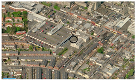
	Station AG Height	3.7
	Station ASL Height	47
	Average Building Height	7.0
	Surface below sensor	Pavement
	Dominant Surface around site	Pave/Buldings
Open Midrise Located on grounds of university	Station 3—South Central
	Station AG Height	3.7
	Station ASL Height	22
	Average Building Height	14.5
	Surface below sensor	Grass/Pavement
	Dominant Surface around site	Grass/Pave/Build
Compact Midrise Located in housing estate in inner city	Station 4—Central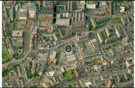
	Station AG Height	4.3
	Station ASL Height	25
	Average Building Height	15
	Surface below sensor	Pavement
	Dominant Surface around site	Pave/Build
Open Lowrise Located on grounds of school	Station 5—South West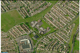
	Station AG Height	1.9
	Station ASL Height	60
	Average Building Height	4.5
	Surface below sensor	Grass/Pave
	Dominant Surface around site	Grass/Pave/Build
Open Lowrise Located on grounds of school	Station 6—North West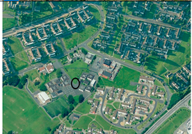
	Station AG Height	1.9
	Station ASL Height	67
	Average Building Height	5.4
	Surface below sensor	Grass/Pave
	Dominant Surface around site	Grass/Pave/Build

The data from these stations were supplemented by air temperature measurements made while traversing the study area by car. The instrument consisted of a class-A ceramic wound Resistance Temperature Detector (RTD) that was fixed within a white plastic cylinder (12 cm long, 2.5 cm diameter). The tube is capped by a short tube that is open at both ends to allow ventilation and the sensor itself sits at the top of the cylinder. This device is described in detail by Hart and Sailor [36]. Four of these instruments were mounted to vehicles (at a height of about 2 m), which allowed us to complete four traverses simultaneously in the study area. Temperature was sampled at a rate of once every 5 s and sufficient time was given prior to beginning each route to allow the sensors to respond to outdoor exposure. The location (and speed) of the vehicle was recorded using GPS and any observations made while the vehicle was stopped were subsequently removed. The paths taken by the vehicles were designed to pass through a variety of LCZ types across the study area including those places where the six fixed stations were located (Figure 3). Each route formed a closed loop and took about one hour to complete; to compensate for the cooling that occurred during an individual traverse, the difference between the temperature recorded at the beginning and the end of the loop was used to estimate the rate of cooling [37]. This rate was applied to all the temperatures recorded during that traverse.

The UHI study presented here is based on measurements made by the fixed stations and traverses mobile sites during a period of mixed weather lasting 7 days (26 August to 1 September 2010). This night-time period (21:00–06:00 h) was associated with low wind-speed and variable cloud coverage (Table 3). Cloud cover over the study area at the beginning of each night of investigation was estimated based on IR-images from EUMETSAT. The period of investigation saw two broad synoptic conditions dominate over the study area. For the first half of the period (night of 26/27–29/30 August) relatively low atmospheric pressure, coupled with high winds and overcast conditions prevailed, whereas the latter part (night of 30 August–1 September) saw the establishment of weak anticyclonic conditions, giving rise to calm winds and clear skies. No significant (>1.0 mm) precipitation was recorded during the period.

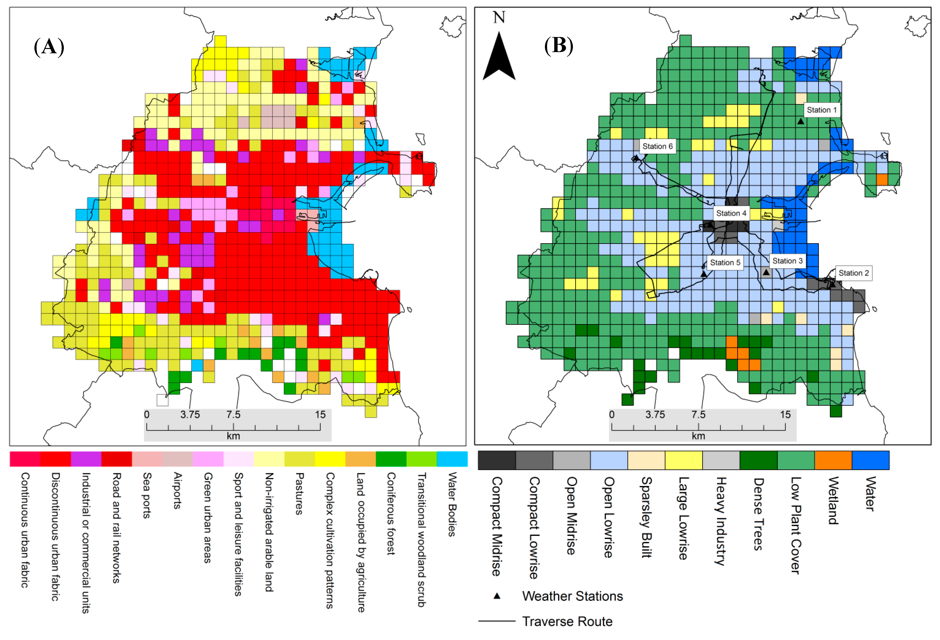
Figure 3. (A) CORINE LULC map (2006) for Dublin City (B) LCZ map derived from LULC and field work, also shown are the four traverse routes and the locations of the six fixed stations.

Figure 3. (A) CORINE LULC map (2006) for Dublin City (B) LCZ map derived from LULC and field work, also shown are the four traverse routes and the locations of the six fixed stations.

Table 3. Mean wind-speed (m∙s⁻¹) from 09:00 to 06:00 h (UTC) for each night at each fixed station (see above). The number in parentheses represents the number of calm periods, that is, 15 min intervals, when no wind-speed was recorded). Airport data is measured at a standard meteorological station outside the built up area at a height of 10 m. Cloud cover was estimated for the entire Dublin region based on IR-images from EUMETSAT at 21:00 h.

Station	LCZ	26-August	27-August	28-August	29-August	30-August	31-August	1-September
1	Low Plants	0.4 (0)	2.3 (0)	4.2 (0)	1.3 (0)	0.2 (10)	0.2 (4)	0.4 (6)
2	Compact Low	0.4 (0)	0.8 (0)	1.4 (0)	0.6 (0)	0.4 (2)	0.3 (2)	0.1 (0)
3	Open Midrise	0.3 (0)	2.5 (0)	2.8 (0)	1.1 (0)	0.7 (0)	0.4 (2)	0.4 (4)
4	Compact Midrise	0.4 (0)	3.8 (0)	1.4 (0)	3.6 (0)	0.8 (0)	0.6 (4)	0.9 (5)
5	Open Lowrise	0.4 (0)	2.1 (0)	3.3 (0)	0.9 (0)	0.6 (0)	0.6 (0)	0.3 (0)
6	Open Lowrise	0.5 (0)	1.8 (0)	2.7 (0)	0.4 (0)	0.9 (0)	0.2 (5)	0.5 (5)
	Dublin Airport	0.7	2.4	3.4	1.1	0.5	0.8	0.8
	Cloud cover	20%	80%	100%	20%	<10%	<10%	15%

Table 3. Mean wind-speed (m∙s⁻¹) from 09:00 to 06:00 h (UTC) for each night at each fixed station (see above). The number in parentheses represents the number of calm periods, that is, 15 min intervals, when no wind-speed was recorded). Airport data is measured at a standard meteorological station outside the built up area at a height of 10 m. Cloud cover was estimated for the entire Dublin region based on IR-images from EUMETSAT at 21:00 h.

Station	LCZ	26-August	27-August	28-August	29-August	30-August	31-August	1-September
1	Low Plants	0.4 (0)	2.3 (0)	4.2 (0)	1.3 (0)	0.2 (10)	0.2 (4)	0.4 (6)
2	Compact Low	0.4 (0)	0.8 (0)	1.4 (0)	0.6 (0)	0.4 (2)	0.3 (2)	0.1 (0)
3	Open Midrise	0.3 (0)	2.5 (0)	2.8 (0)	1.1 (0)	0.7 (0)	0.4 (2)	0.4 (4)
4	Compact Midrise	0.4 (0)	3.8 (0)	1.4 (0)	3.6 (0)	0.8 (0)	0.6 (4)	0.9 (5)
5	Open Lowrise	0.4 (0)	2.1 (0)	3.3 (0)	0.9 (0)	0.6 (0)	0.6 (0)	0.3 (0)
6	Open Lowrise	0.5 (0)	1.8 (0)	2.7 (0)	0.4 (0)	0.9 (0)	0.2 (5)	0.5 (5)
	Dublin Airport	0.7	2.4	3.4	1.1	0.5	0.8	0.8
	Cloud cover	20%	80%	100%	20%	<10%	<10%	15%

2.5. Analysis

The data from both the fixed and mobile stations were processed and examined within the context of the LCZ scheme. Mean night-time (21:00–06:00 h) temperature for each of the fixed stations (T_F(i)) was obtained and its relative anomaly ( ) was calculated as the difference between the station mean and the group mean,

(3)

Each temperature value from the traverses (T_M) was assigned a LCZ code based on the recorded location of the vehicle at the time and the LCZ map (Figure 3). These data were subsequently used to generate descriptive statistics for each LCZ type and define our UHI (T_LCZ) as done in Stewart et al. [38].

3. Results

3.1. Unfavorable UHI Conditions (26–29 August)

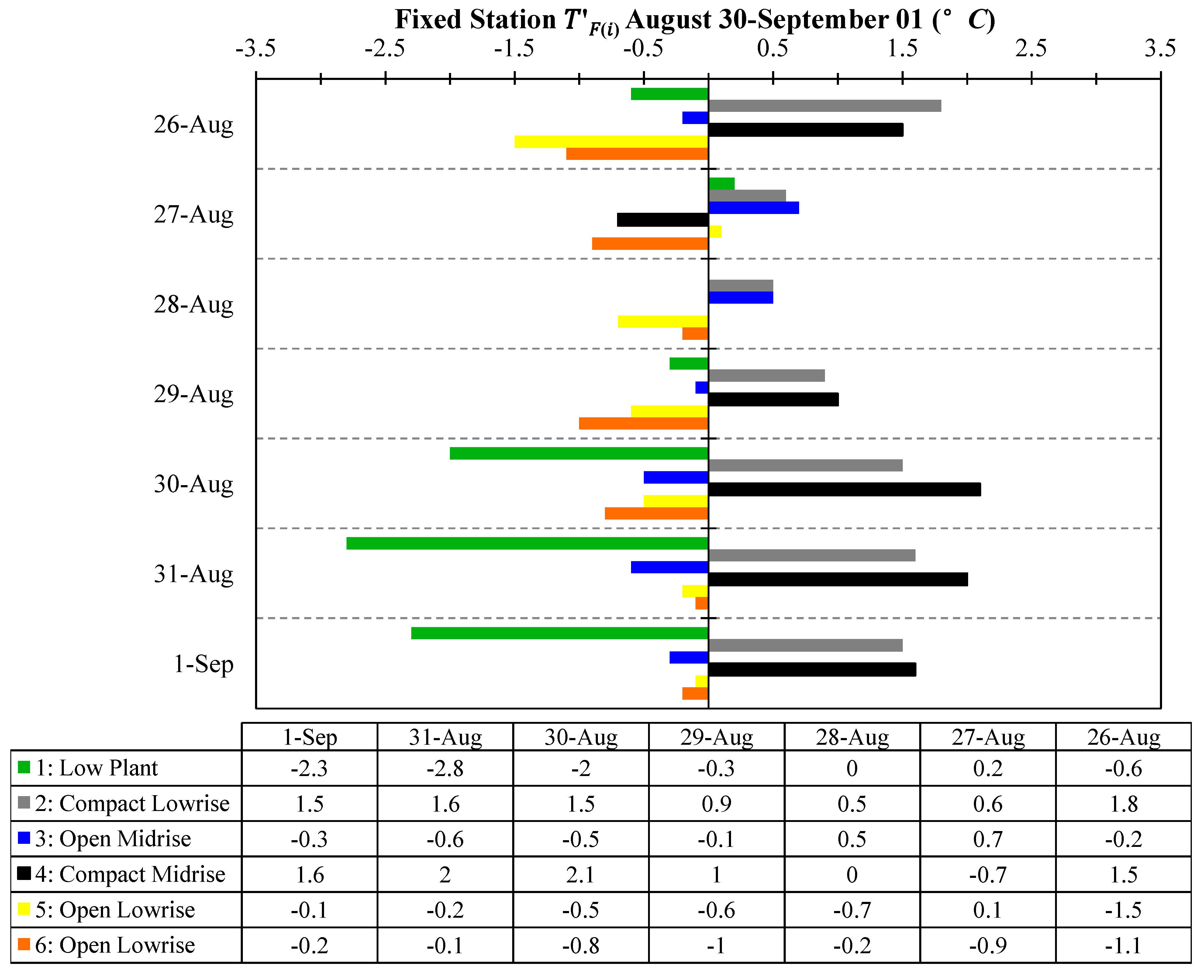
Relatively strong west to south-westerly winds were present during the first part of the week of investigation (26–29 August): mean wind speed at night ranged from 0.4 to 4.2 m∙s⁻¹ with high fraction of cloud cover over the city. These conditions are associated with low pressure giving rise to relatively inclement conditions compared to the latter part of the period. Generally, only slightly elevated air temperatures ( < 1.0 °C) were present in compact urban LCZ (stations 2 and 4); however, the direction of this signal remained positive throughout the period (see Figure 4). In relation to stations 5 and 6, which can be described as the suburban stations (LCZ 6), generally both exhibited a negative (0.2–1.0 °C) signal relative to the group mean.

The lack of significant temperature variation among the stations during the first part of the period implies greater mixing across the LCZ. It is clear the unsettled conditions served to mitigate strong UHI development as has been shown in other studies [26,27]. A pattern of gentle thermal gradients is thus anticipated to have developed across the city and overall a weakly developed UHI formed on these nights. This corresponds with research elsewhere on the impact of cloud coverage and wind speed on diminishing UHI development [39].

3.2. Favorable UHI Conditions (30 August–1 September)

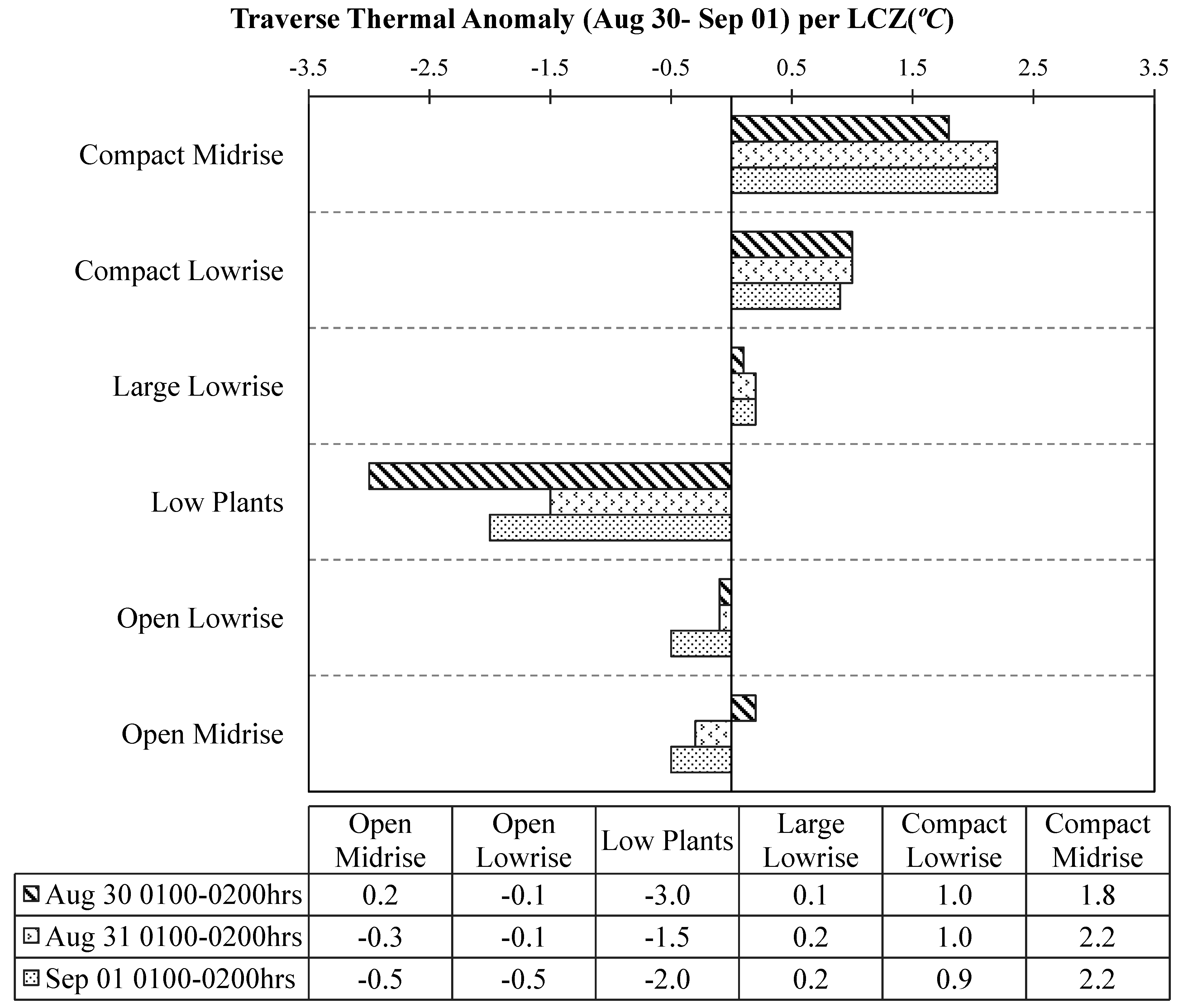
Increasingly settled anticyclonic conditions dominated for the latter part of the week of investigation. Wind-speed at night was 0.1–0.9 m∙s⁻¹ across the city (Table 3) and there were short periods of calm at some stations. When coupled with open skies (cloud coverage <10%) these conditions suggest favorable UHI development. Unlike the beginning of the period, a clear distinction between LCZ can be identified in . The largest T_LCZ (4.8 °C) difference occurred between station 1 (LCZ D Low Plants) and station 4 (LCZ 2 Compact Midrise) on August 31. Throughout the latter part of the period, these two stations exhibited the largest difference as would be expected a priori. In terms of the traverse data, a difference of ~4.3 °C between the compact LCZ and non-urban LCZ between 01:00 and 02:00 h was recorded across all three nights (based on ~6000 sampled points) though the largest difference recorded was on 29 August rather than 31 August as was the case with the fixed stations. Nevertheless, the consistency of the signal suggests the effect of building density and artificial surface coverage on air temperatures was efficiently captured by the routes chosen. Differences between the periphery (beyond the suburban fringe) and urban core are expected to have been higher—though these areas were not explicitly sampled due to the range that could be covered in 60 min travelling time.

Figure 4. Nocturnal (21:00–06:00 h UTC) Thermal Anomalies ( ) for the six fixed stations for night of 26/27 August to night of 1/2 September. Each station (1–6) is represented by a bar below and identified by the LCZ in which they are placed. Note the latter part of the week (30 August–1 September) show the largest T_LCZ, i.e., the range covering the min to max.

Figure 4. Nocturnal (21:00–06:00 h UTC) Thermal Anomalies ( ) for the six fixed stations for night of 26/27 August to night of 1/2 September. Each station (1–6) is represented by a bar below and identified by the LCZ in which they are placed. Note the latter part of the week (30 August–1 September) show the largest T_LCZ, i.e., the range covering the min to max.

A comparison between temperature measurements at both the fixed stations and mobile systems are not easily made as the latter sample from the variety of microclimates within the LCZ at 5 s intervals, whereas the former samples from a single representative microclimate at 30 min intervals. For 30 August, we compared mobile temperature measurements made within 150 m of the fixed sites with those made at the nearest station; the results indicate a range of difference (−0.1–0.4 °C) with a small positive bias (+0.2 °C) on average, which might suggest that the stations are located in more “urban” warmer microclimates than the traverses. Nevertheless, the pattern of differences between the LCZ types is consistent for both fixed and mobile systems.

Figure 5. Nocturnal (UTC 01:00–02:00 h) Thermal Anomalies derived from traverse data for stable nights. Each night (30 August–1 September) is represented by a bar below.

Figure 5. Nocturnal (UTC 01:00–02:00 h) Thermal Anomalies derived from traverse data for stable nights. Each night (30 August–1 September) is represented by a bar below.

Figure 4 shows values for the period 21:00–06:00 h; note that the stations located within LCZ with the highest impervious/built coverage (stations 2 and 4) consistently exhibit positive thermal anomalies each night throughout the week of observation compared to stations with higher pervious (vegetated) coverage. Moreover, towards the latter part of the week, again when settled conditions began to dominate, the relationship between station 1, 2 and 4 which represent low and high levels of urban development respectively becomes apparent. The effect of extensive vegetation can be seen in the open lowrise and low plant LCZ stations. Similar results are seen in the traverse data (Figure 5) which examined nocturnal temperatures in the latter part of the week in more detail. These values are derived from LCZ at different geographic locations across the domain rather than the fixed stations which each observe one location. They compare favorably with the fixed station results in terms of the direction of the thermal signal. A consistent trend over the three nights of above average temperatures were recorded in the most urbanized LCZ classes in Dublin, whereas the non-urban and less-urban LCZ exhibited below average temperatures across the domain. Again, the magnitudes between the fixed station and traverses appear to show slight disparity. For the traverses, 30 August exhibited the strongest T_LCZ difference which occurred between Compact Midrise (inner-city locations) and Low Plant LCZ (non-urban areas) though this relationship was consistent on all three nights. The ranking of the LCZ (in terms of + or − thermal signals) sampled by the traverses appears to follow a logical pattern whereby areas containing a larger coverage of artificial materials exhibited positive thermal signals similar to modeling results obtained during the development of the LCZ system [38].

Coupled with the fixed station results, this appears to demonstrate the effectiveness of the LCZ classification in terms of its design towards capturing variations in the energy budget leading to the UHI. Table 4 summarizes the traverse results for 30 August across all the sampled areas. Generally, LCZ can be distinguished well using observed T_Mean and T_Max values; however when examining T_Min values, the relative difference seems to be between compact and non-compact LCZ—this may have arisen due to the transitions from one area to another i.e., LCZ zone boundaries which are microscale (10–10² m) whereas our LCZ map is based on the local scale (10³ m).

Table 4. Summary of Traverse Results: Shown are number of sampled areas with particular LCZ class (same route followed for 30 August–1 September) along with T_MEAN, T_MIN and T_MAX (°C) for 30 August between UTC 01:00–02:00 h. After the removal of stationary points n = 2192.

LCZ	Number of Areas Sampled (km2)	TMEAN	TMIN	TMAX
Compact Midrise	7	10.6	8.1	12.9
Compact Lowrise	6	9.9	8.4	12.5
Open Midrise	1	7.7	6.9	8.1
Open Lowrise	70	8.2	6.0	11.0
Large Lowrise	12	8.9	6.2	10.4
Low Plants	17	6.9	6.0	8.5

Table 4. Summary of Traverse Results: Shown are number of sampled areas with particular LCZ class (same route followed for 30 August–1 September) along with T_MEAN, T_MIN and T_MAX (°C) for 30 August between UTC 01:00–02:00 h. After the removal of stationary points n = 2192.

LCZ	Number of Areas Sampled (km2)	TMEAN	TMIN	TMAX
Compact Midrise	7	10.6	8.1	12.9
Compact Lowrise	6	9.9	8.4	12.5
Open Midrise	1	7.7	6.9	8.1
Open Lowrise	70	8.2	6.0	11.0
Large Lowrise	12	8.9	6.2	10.4
Low Plants	17	6.9	6.0	8.5

4. Discussion

4.1. Inter-LCZ Relationships

The relationship between different LCZ air temperatures derived here corresponds well with recent work done in cities elsewhere. For instance, Fenner et al. [40] found temperature differences of approximately 1 °C (K) in the decadal average during summer nights between stations located in dense-trees (LCZ A) and open lowrise (LCZ 6) around Berlin, Germany. The closest analogous value derived here was between low plant cover (LCZ D) and open lowrise (LCZ 6) which reached a maximum difference of 1.5 °C based on the traverse results. The average difference based on the in-situ stations for the week considered here was 1.6 °C.

Leconte et al. [41] examine inter-LCZ relationships using the mobile traverse method in Nancy, France. The inter-LCZ differences derived here also show close resemblance to their results which compare paired LCZ types approximately 3 h after sunset. For instance, at our in-situ stations the difference between LCZ 6 and LCZ D during the favourable UHI conditions was ~2.1 °C, while the corresponding magnitude taken from [41] was 2.4 °C; a similar value (~2.0 °C) was found here in the traverse data. Moreover, there is correspondence between compact midrise (LCZ 2) in Dublin and Nancy which are consistently warmer, whereas LCZ D is consistently cooler in both studies. The intra-urban LCZ differences also correspond well with [41]. Based on our traverses results here, the mean difference between LCZ 2 and LCZ 6 was 2.3 °C, approximately 0.5 °C higher than the value reported for Nancy. The mean difference for same LCZ pair from the in-situ stations during the favourable UHI conditions was ~2.2 °C. Table 5 compares the results for Dublin with these mentioned studies. It is important to highlight that direct comparison with these studies should be interpreted with caution in light of the differences in instrumentation, study period, sitting and background climate. The exact nature of LCZ classes in each study may also differ in terms of land use and building materials.

Table 5. Comparison of T_LCZx–T_LCZy from this study to analogous results from other studies. Values given are in K. Where no analogous value could be obtained “---” appears. The mobile and fixed values for Dublin are averages from the three nights of observations during favorable UHI conditions. Fixed LCZ 6 values are taken across the two stations.

	Dublin		Analogous Result from Other Cities
Intra-urban	Fixed	Mobile	Berlin 1	Nancy 2	Nagano 3	Vancouver 4	Uppsala 5
LCZ2-LCZ3	0.5	1.1	---	---	1.7	---	---
LCZ2-LCZ6	2.2	2.3	---	1.8	2	* 2.3	** 1.5
Inter-Urban
LCZ2-LCZD	4.2	4.2	---	4.4	3.2	* 6.3	3.3
LCZ3-LCZD	3.9	3.1	** 1.5	---	1.5	---	---
LCZ6-LCZD	2	1.9	0.8	2.4	1.2	4	** 1.8

¹ Reported decadal average, Table 2 in [40]; ² Average differences during nighttime period approximately 3 h after sunset, Table 1 in [41]; ³ Reported Annual departures used, Figure 3 in [38]; ⁴ Nocturnal traverses during November 1999, Figure 5 in [38]; ⁵ Reported Annual departures used, Figure 8 in [38]; * Value for LCZ1 used in place of LCZ 2; ** Value for LCZ5 used in place of LCZ 6 (in place of LCZ 3 for Berlin).

Table 5. Comparison of T_LCZx–T_LCZy from this study to analogous results from other studies. Values given are in K. Where no analogous value could be obtained “---” appears. The mobile and fixed values for Dublin are averages from the three nights of observations during favorable UHI conditions. Fixed LCZ 6 values are taken across the two stations.

	Dublin		Analogous Result from Other Cities
Intra-urban	Fixed	Mobile	Berlin 1	Nancy 2	Nagano 3	Vancouver 4	Uppsala 5
LCZ2-LCZ3	0.5	1.1	---	---	1.7	---	---
LCZ2-LCZ6	2.2	2.3	---	1.8	2	* 2.3	** 1.5
Inter-Urban
LCZ2-LCZD	4.2	4.2	---	4.4	3.2	* 6.3	3.3
LCZ3-LCZD	3.9	3.1	** 1.5	---	1.5	---	---
LCZ6-LCZD	2	1.9	0.8	2.4	1.2	4	** 1.8

¹ Reported decadal average, Table 2 in [40]; ² Average differences during nighttime period approximately 3 h after sunset, Table 1 in [41]; ³ Reported Annual departures used, Figure 3 in [38]; ⁴ Nocturnal traverses during November 1999, Figure 5 in [38]; ⁵ Reported Annual departures used, Figure 8 in [38]; * Value for LCZ1 used in place of LCZ 2; ** Value for LCZ5 used in place of LCZ 6 (in place of LCZ 3 for Berlin).

Finally, the relationship between all sampled LCZ in Dublin as derived by the traverses during three ideal nights (Figure 5) is remarkably similar to the ranking derived in the Nagano basin and reported in [38]. Based on five nights of observations during May–June, the ranking of urban LCZ compared to LCZ D in Nagano is consistent with the ranking found here in that the magnitude (T_{LCZ X}−T_{LCZ D}) is highest in LCZ 2 for both cities; the next highest magnitude is found with LCZ 3 and after this LCZ 6.

4.2. Mapping Dublin’s Canopy-Layer UHI

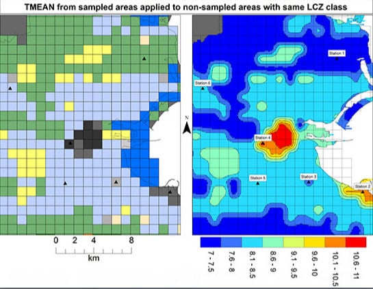
Based on the results from the LCZ analysis, it seems reasonable to assume that the T_Mean values from the sampled grid cells could be attributed to the non-sampled grid cells based on their LCZ type. Figure 6B shows the results for 30 August, when the measured UHI was strongest. To aid with visual interpretation of the results the predicted air temperatures were interpolated using Inverse Distance Weighting and the resulting temperature map is shown in Figure 6B. Generally, the spatial pattern of 2 m T_Mean that we deried utilizing the LCZ follows previous observational work on Dublin’s UHI [26,27] though the relationship between built form and nocturnal temperature is now clearer, with the highest values occurring in the compact LCZ classes (corresponding to the inner city area) that have little vegetative cover. The large urban park directly west of the inner-city is shown as a cool area, much like the non-urban areas to the north and south of the built-up area. The LCZ scheme provides a strong framework in which to conduct basic urban climate investigations and formulate a basic description of UHI. Though, given the level of detail contained within the classification scheme itself, it is reasonable to assume the scheme has potential for more complex investigation such as the derivation of the energy budget for modeling applications [42].

Figure 6. (A) LCZ map (legend same as in Figure 3B) zoomed in for comparison (B) T_MEAN 01:00–02:00 h 30 August 2010 (values given in Table 4) from sampled areas applied to non-sampled areas with the same LCZ class

Figure 6. (A) LCZ map (legend same as in Figure 3B) zoomed in for comparison (B) T_MEAN 01:00–02:00 h 30 August 2010 (values given in Table 4) from sampled areas applied to non-sampled areas with the same LCZ class

4.3. Mitigating Factors

The main factors found to affect Dublin’s UHI development and the distinction between LCZ classes were related to synoptic conditions which serve to limit UHI development, namely wind speed and cloud coverage. Sweeney [26] concludes that wind speed is the leading factor in mitigating strong UHI development given the geographic sitting of Dublin city. Moreover, he identifies the link between wind speed and the displacement of air temperatures leeward of the dominant wind direction. Sweeney utilised city size (or rather population as a proxy for city size) to determine the critical threshold, that is, the wind speed at which the UHI becomes null as the action of advection instigates mixing beyond which the urban effect cannot be detected by standard instruments. As outlined in Oke and Hannell [43] almost four decades ago, this can be approximated as;

U_crit= 3.4 log (P) − 11.6

(4)

where U_crit is the threshold wind speed (m∙s⁻¹) and (P) is population. Sweeney estimated that Dublin’s UHI is diminished at wind speeds of over 7 m∙s⁻¹. Graham [27] found that at wind speeds above 5 m∙s⁻¹ the UHI intensity in Dublin was <3 °C. Here at the highest recorded wind speeds of between 2.5 and 4.2 m∙s⁻¹, the peak T_LCZ was reduced to 1.0 °C, whereas at the lowest wind speed 0–0.7 m∙s⁻¹ T_LCZ>4.0 °C. Graham [27] found with cloud cover greater than 4 okta (~50%) UHI intensity was <2 °C and >4 °C under calm clear conditions. Similar values were obtained here during anticyclonic conditions from 30 August to 1 September with recorded UHI intensities of 4.8 °C, 3.9 °C and 4.3 °C, respectively, from the traverse results. As we did not conduct traverses during the cyclonic conditions (as was done in both previous studies), we are unable to quantify the exact spatial displacement of the UHI, but we might expect as per Sweeney [26] that air temperatures were displaced leeward of the dominant wind direction on these night diminishing T_LCZ differences.

5. Conclusions

Local Climate Zones (LCZ) describe the landscape in terms of the surface elements that give rise to near-surface air temperature differences. This study has shown the value of LCZ mapping as an initial step that aids in the design, implementation and interpretation of an urban heat island (UHI) investigation. In this study of Dublin, it was used to help researchers plan and deploy a small meteorological network and conduct a set of traverse routes that recorded air temperature during ideal weather conditions for strong UHI formation. Under ideal synoptic conditions examined here, a maximum nocturnal air temperature difference of more than 4 °C was detected between urban and non-urban LCZ (T_{LCZ 2}–T_{LCZ D}) beyond the urban fringe. The use of the LCZ map has allowed us to map the pattern of the UHI across the city efficiently. The results of the study indicate that the LCZ type is a significant control on the magnitude of the UHI and that it can be used to make reasonable inferences about the temperature signal in urban neighborhoods where there are no observations. The LCZ scheme provides a useful framework for designing a UHI experiment and explaining intra-urban variation, especially under ideal weather for UHI formation.

References

- Oke, T.R. The distinction between canopy and boundary-layer urban heat islands. Atmosphere 1976, 14, 269–277. [Google Scholar]
- Mills, G. Luke Howard and the climate of London. Weather 2008, 63, 153–157. [Google Scholar]
- Jauregui, E. Heat Island Development in Mexico City. Atmos. Environ. 1997, 31, 3821–3831. [Google Scholar]
- Magee, N.; Curtis, J.; Wendler, G. The urban heat island effect at Fairbanks, Alaska. Theor. Appl. Climatol. 1999, 64, 39–47. [Google Scholar]
- Hicks, B.; Callahan, W.; Hoekzema, M. On the heat islands of Washington, DC, and New York city, NY. Bound. Layer Meteorol. 2010, 135, 291–300. [Google Scholar]
- Kim, Y.; Baik, J. Maximum urban heat island intensity in Seoul. J. Appl. Meteorol. 2002, 41, 651–659. [Google Scholar]
- Fortuniak, K.; Klysik, K.; Wibig, J. Urban–rural contrasts of meteorological parameters in Lodz. Theor. Appl. Climatol. 2006, 84, 91–101. [Google Scholar]
- Kolokotroni, M.; Giridharan, R. Urban heat island intensity in London: An investigation of the impact of physical characteristics on changes in outdoor air temperature during summer. Sol. Energy 2008, 82, 986–998. [Google Scholar]
- Oke, T.R. The energetic basis of the urban heat island. Q. J. R. Meteorol. Soc. 1982, 455, 1–24. [Google Scholar]
- Oke, T.R. Towards better scientific communications in urban climate. Theor. Appl. Climatol. 2006, 84, 179–190. [Google Scholar]
- Nunez, M.; Oke, T.R. The energy balance of an urban canyon. J. Appl. Meteorol. 1977, 16, 11–19. [Google Scholar]
- Kondo, A.; Ueno, M.; Kaga, A.; Yamaguchi, K. The influence of urban canopy configuration on urban albedo. Bound. Layer Meteorol. 2001, 100, 225–242. [Google Scholar]
- Grimmond, C.S.B.; Oke, T.R. Comparison of heat fluxes from summertime observations in the suburbs of four North American cities. J. Appl. Meteorol. 1995, 34, 873–889. [Google Scholar]
- Ichinose, T.; Shimodozono, K.; Hanaki, K. Impact of anthropogenic heat on urban climate in Tokyo. Atmos. Environ. 1999, 33, 3897–3909. [Google Scholar]
- Offerle, B.; Grimmond, C.S.B.; Fortuniak, K. The energy balance of a central European city centre. Int. J. Climatol. 2005, 25, 1405–1419. [Google Scholar]
- Grimmond, C.S.B.; Oke, T.R. Turbulent heat fluxes in urban areas: Observations and a Local-Scale Urban Meteorological Parameterization Scheme (LUMPS). J. Appl. Meteorol. 2002, 41, 792–810. [Google Scholar]
- Grimmond, C.S.B.; Oke, T.R. Heat storage in urban areas: Local-scale observations and evaluation of a simple model. J. Appl. Meteorol. 1999, 38, 922–940. [Google Scholar]
- Sailor, D.J. Anthropogenic heat and moisture emissions in the urban environment. In Proceedings of the Seventh International Conference on Urban Climate, Yokohama, Japan, 29 June–3 July 2009.
- Stewart, I.D.; Oke, T.R. Local climate zones for urban temperature studies. Bull. Am. Meteorol. Soc. 2012, 93, 1879–1900. [Google Scholar]
- Stewart, I.D.; Oke, T.R. Overview of the local climate zone classification system: Origins, development, and application to urban heat islands. In Proceedings of the Association of American Geographers Annual Meeting, Seattle, WA, USA, 12–16 April 2011.
- Kovács, A.; Németh, Á. Tendencies and differences in human thermal comfort in distinct urban areas in Budapest, Hungary. Acta Climatol. Chorol. 2012, 46, 115–124. [Google Scholar]
- Puliafito, S.; Bochaca, F.; Allende, D.; Fernandez, R. Green areas and microscale thermal comfort in arid environments: A case study in Mendoza, Argentina. Atmos. Clim. Sci. 2013, 3, 372–384. [Google Scholar]
- Stewart, I.D. A systematic review and scientific critique of methodology in modern urban heat island literature. Int. J. Climatol. 2011, 31, 200–217. [Google Scholar]
- Walsh, S. A Summary of Climate Averages for Ireland 1981–2010. Available online: http://www.met.ie/climate-ireland/30year-averages.asp (accessed on 24 September 2014).
- Central Statistics Office (CSO). Ireland (2012) Census of Ireland 2011. Available online: http://www.cso.ie/en/census/ (accessed on 18 April 2013).
- Sweeney, J. The urban heat island of Dublin city. J. Ir. Geogr. 1987, 20, 1–10. [Google Scholar]
- Graham, E. The urban heat island of Dublin city during the summer months. J. Ir. Geogr. 1993, 26, 43–57. [Google Scholar]
- Unger, J.; Lelovics, E.; Gál, T. Local climate zone mapping using GIS methods in Szeged. Hung. Geogr. Bull. 2014, 63, 29–41. [Google Scholar]
- Bechtel, B. Multitemporal Landsat data for urban heat island assessment and classification of local climate zones. In Proceedings of the 2011 Joint Urban Remote Sensing Event (JURSE), Munich, Germany, 11–13 April 2011; pp. 129–132.
- Bechtel, B.; Daneke, C. Classification of local climate zones based on multiple earth observation data. IEEE J. Sel. Top. Appl. Earth Obs. Remote Sens. 2012, 5, 1191–1202. [Google Scholar]
- EEA. CLC2006 Technical Guidelines. Available online: http://www.eea.europa.eu/publications/COR0-landcover (accessed on 24 September 2014).
- Arnfield, J. Two Decades of Urban Climate Research: A review of turbulence, exchanges of energy and water, and the urban heat island. Int. J. Climatol. 2003, 23, 1–26. [Google Scholar]
- Oke, T.R. Urban Observation. Chapter 11 in Guide to Meteorological Instruments and Methods of Observation, 7th ed.; No. 8; WMO: Geneva, Switzerland, 2008. [Google Scholar]
- Chandler, T.J. City growth and urban climates. Weather 1964, 19, 170–171. [Google Scholar]
- Runnalls, K.E.; Oke, T.R. A technique to detect microclimatic inhomogeneities in historical records of screen-level air temperature. J. Clim. 2006, 19, 959–978. [Google Scholar]
- Hart, M.; Sailor, D.J. Assessing causes in spatial variability in urban heat island magnitude. In Proceedings of the Seventh Symposium on the Urban Environment, San Diego, CA, USA, 10–13 September 2007.
- Tso, C.P. A survey of urban heat island studies in two tropical cities. Atmos. Environ. 1996, 30, 507–519. [Google Scholar]
- Stewart, I.D.; Oke, T.R.; Krayenhoff, E.S. Evaluation of the “local climate zone” scheme using temperature observations and model simulations. Int. J. Climatol. 2014, 34, 1062–1080. [Google Scholar]
- Morris, C.J.G.; Simmonds, I.; Plummer, N. Quantification of the influences of wind and cloud on the nocturnal urban heat island of a large city. J. Appl. Meteorol. 2001, 40, 169–182. [Google Scholar]
- Fenner, D.; Meier, F.; Scherer, D.; Polze, A. Spatial and temporal air temperature variability in Berlin, Germany, during the years 2001–2010. Urban Clim. 2014. [Google Scholar] [CrossRef]
- Leconte, F.; Bouyer, J.; Claverie, R.; Pétrissans, M. Using local climate zone scheme for UHI assessment: Evaluation of the method using mobile measurements. Build. Environ. 2014. [Google Scholar] [CrossRef]
- Ching, J. A perspective on urban canopy layer modeling for weather, climate and air quality applications. J. Urban Clim. 2013, 3, 13–39. [Google Scholar]
- Oke, T.R.; Hannell, F.G. The Form of the Urban Heat Island in Hamiliton, Canada; Technical Note; World Meteorological Organisation: Geneva, Switzerland, 1970; Volume 108, pp. 113–126. [Google Scholar]
© 2014 by the authors; licensee MDPI, Basel, Switzerland. This article is an open access article distributed under the terms and conditions of the Creative Commons Attribution license (http://creativecommons.org/licenses/by/4.0/).
Share and Cite
MDPI and ACS Style
Alexander, P.J.; Mills, G. Local Climate Classification and Dublin’s Urban Heat Island. Atmosphere 2014, 5, 755-774. https://doi.org/10.3390/atmos5040755
AMA Style
Alexander PJ, Mills G. Local Climate Classification and Dublin’s Urban Heat Island. Atmosphere. 2014; 5(4):755-774. https://doi.org/10.3390/atmos5040755
Chicago/Turabian StyleAlexander, Paul J., and Gerald Mills. 2014. "Local Climate Classification and Dublin’s Urban Heat Island" Atmosphere 5, no. 4: 755-774. https://doi.org/10.3390/atmos5040755