Genetic Programming for the Downscaling of Extreme Rainfall Events on the East Coast of Peninsular Malaysia

Abstract

A genetic programming (GP)-based logistic regression method is proposed in the present study for the downscaling of extreme rainfall indices on the east coast of Peninsular Malaysia, which is considered one of the zones in Malaysia most vulnerable to climate change. A National Centre for Environmental Prediction reanalysis dataset at 42 grid points surrounding the study area was used to select the predictors. GP models were developed for the downscaling of three extreme rainfall indices: days with larger than or equal to the 90th percentile of rainfall during the north-east monsoon; consecutive wet days; and consecutive dry days in a year. Daily rainfall data for the time periods 1961–1990 and 1991–2000 were used for the calibration and validation of models, respectively. The results are compared with those obtained using the multilayer perceptron neural network (ANN) and linear regression-based statistical downscaling model (SDSM). It was found that models derived using GP can predict both annual and seasonal extreme rainfall indices more accurately compared to ANN and SDSM.

1. Introduction

Climate change due to global warming will modify the climate in terms of both the mean and variability of rainfall [1,2]. Small changes in rainfall variability and the mean can produce relatively large changes in the probability of extreme rainfall events [3,4]. As the primary impacts of climate change on human life, environments, economies and societies result from extreme events, changes in extreme weather events due to global warming have become a major concern in recent years [2,5,6]. Therefore, reliable projection of future changes in extreme indices at the local scale is a major challenge in any climate region.

General circulation models (GCMs) are generally designed to simulate the present climate and project the future climate. However, GCMs cannot be used to project local- and regional-scale climates and their changes, because of their coarse spatial resolutions. Therefore, GCM simulations are downscaled into much finer spatial resolution for climate change impact studies at local and regional scales [7]. Two major downscaling approaches are often used: dynamical downscaling methods that are based on high-resolution regional climate models [8,9] and statistical downscaling methods based on some established statistical relationships between large-scale atmospheric variables (predictors) and local climate variables (predictands) [10,11]. Compared to dynamic downscaling, statistical downscaling requires simple computational skills to downscale GCM outputs in order to understand possible future changes in climate at the local scale [12].

A number of studies on downscaling extreme indices has been carried out in recent years [12,13,14,15,16,17]. However, this is still new in Malaysia and Southeast Asian countries, where studies of statistical downscaling have focused mainly on mean climate. Logistic regression is a popular technique for classifying information into two mutually exclusive and exhaustive categories [18]. It has been used for the downscaling of extreme rainfall indices in a number of research papers [19,20,21]. Logistic regression creates decision trees for the creation of decision rules. One of the main drawbacks of conventional logistic regression-based statistical downscaling procedures is that the performance of such models depends on theoretical assumptions and data restrictions. Furthermore, conventional statistical logistic regression methods show poor performance when the variable of interest is precipitation; the predictor/predictand relationships are very complex, and conventional downscaling methods may not work satisfactorily [22]. Genetic programming (GP) is a kind of non-parametric regression, which can relate the predictors and predictands and provide a predictive model identical to the analytical optimal solution when interrelationships between variables are poorly understood [23,24,25,26,27,28,29]. Genetic-based statistical logistic regression offers a clear advantage over the standard statistical logistic regression method [30,31]. It generates a set of logical expressions describing the structure of the data through iterative subsumption and probabilistically picks the most appropriate set to allow the system to predict in non-deterministic situations, while the achievement of this is not possible with current statistical logistic regression. Thus, the objective of the present study was to use a GP-based logistic regression method for the downscaling of rainfall extremes. The method is tested for the east coast of Peninsular Malaysia.

Three extreme rainfall indices that are important for the economy and livelihood of the population of the east coast of Peninsular Malaysia were downscaled: heavy rainfall days (days with larger than or equal to the 90th percentile of rainfall) during the north-east (NE) monsoon; consecutive dry days; and consecutive wet days in a year. The east coast of Peninsular Malaysia is one of the zones most vulnerable to climate change in the country [32]. It has been reported that extreme rainfall events have increased in Peninsular Malaysia in recent years [32,33,34]. Floods triggered by heavy rainfall are a major hydrological disaster, and almost every year, phenomena occur in the area. Deni et al. [33] reported that rainfall intensity increased in much of Peninsular Malaysia during the south-west (SW) monsoon. During the NE monsoon, total rainfall, the frequency of extreme rainfall events and rainfall intensity increased all over the peninsula [34]. It is anticipated that variability in inter-annual and inter-seasonal rainfall due to climate change will cause more hydrologic extremes on the east coast of Peninsular Malaysia and make people’s livelihoods and local infrastructure more vulnerable. Therefore, downscaling extreme rainfall indices is very important for the creation of rational countermeasures in the context of climate change.

2. Methodology

2.1. Data and Sources

Rainfall data recorded at three stations, namely Besut, Dungun and Kemaman, on the east coast of Peninsular Malaysia were used to downscale the extreme rainfall indices using GP. The location of rainfall stations on the map of Peninsular Malaysia is shown in Figure 1a. The climate of the area can be loosely divided into four seasons: the NE monsoon from October to February; the SW monsoon from April to August; and two inter-monsoonal transitional periods in March and September. The east coast is considered as the wet belt of Peninsular Malaysia, with an annual rainfall of 2800 mm. Heavy rainfall on the east coast of Peninsular Malaysia is usually associated with the NE monsoon. Maximum precipitation usually occurs during the months of November and December. On the other hand, cloudless skies are observed during the SW monsoon. The topographic map of the study area, prepared using the Advanced Spaceborne Thermal Emission and Reflection Radiometer Global Digital Elevation Model, is shown in Figure 1b. The elevation in the area varies from −4 m on the narrow coastal plain to 2270 m in the interior mountainous region.

Daily rainfall data series for the time period 1961–2000 recorded at three locations in the study area were obtained from the Department of Irrigation and Drainage Malaysia. The predictors were obtained from the National Centre for Environmental Prediction (NCEP) reanalysis dataset [35]. Climate model data represent an aggregate over a grid box, and therefore, NCEP data are not an ideal representation of precipitation extremes computed from averages over stations. However, a number of studies have reported that the relationship between the extremes of gridded climatological datasets and observed point-level data from weather stations can be used to predict point-level extreme behavior from future runs of climate models [36,37,38,39,40,41].

Data quality control is a necessary step before the calculation of indices, because erroneous outliers can seriously impact index calculation and trends [42]. A number of quality control checks were carried out to identify errors, such as precipitation values below 0 mm, rainfall higher than 250 mm, more than 20 consecutive dry days during the NE monsoon and more than 20 consecutive wet days during the SW monsoon. Histograms of the data were also created to reveal problems in the dataset as a whole [43]. A Student’s t-test was used to test the difference in the means between the two segments of the dataset to ensure the homogeneity of data. Differences between the sub-set series are not significant at the 95% level of confidence for any station.

Figure 1. (a) Location of the rain gauge stations in Peninsular Malaysia; (b) terrain map of the study area.

Figure 1. (a) Location of the rain gauge stations in Peninsular Malaysia; (b) terrain map of the study area.

Three extreme rainfall indices were computed for the present study. Table 1 provides descriptions of the indices. The indices were calculated on a seasonal or annual basis. In computing the percentile-based index, the percentile was calculated from the reference period 1961–1990, which is a normal climate period as defined by the World Meteorological Organization [44]. Heavy rainfall on the east coast of Peninsular Malaysia is usually associated with the NE monsoon. Therefore, only heavy rainfall days (the days with larger than or equal to the 90th percentile of rainfall) during the NE monsoon were downscaled in the present study.

Table 1. Definitions of precipitation indices used in the present study.

Index	Description	Unit
R90	Total number of days during NE monsoon in a year with rainfall ≥90th percentile of 1961–1990 daily rainfall	day
CDD	Maximum number of consecutive dry days (rainfall = 0) in a year	day
CWD	Maximum number of consecutive wet days (rainfall > 0) in a year	day

Table 1. Definitions of precipitation indices used in the present study.

Index	Description	Unit
R90	Total number of days during NE monsoon in a year with rainfall ≥90th percentile of 1961–1990 daily rainfall	day
CDD	Maximum number of consecutive dry days (rainfall = 0) in a year	day
CWD	Maximum number of consecutive wet days (rainfall > 0) in a year	day

2.2. Selection of Predictors

One of the major challenges in climate downscaling, especially in downscaling extreme rainfall indices, is the selection of appropriate predictors. It is expected that predictors should be highly correlated with extreme rainfall indices. Furthermore, the predictors should be accurately projected by available GCMs for the future projection of climate. There are no general guidelines for the selection of predictors in different parts of the world, and therefore, a comprehensive search of predictors is necessary [45]. Twenty-six NCEP variables that are usually projected by various climate models, including the Hadley Centre Climate Model (HadCM), were used in the present study for the selection of predictors. The description of 26 NCEP variables is given in Table 2.

Table 2. Description of 26 NCEP variables used for predictor selection.

No.	Variables	Description	No.	Variables	Description
1	mslp	Mean sea level pressure	14	p5zh	500 hPa divergence
2	p_f	Surface airflow strength	15	p8_f	850 hPa airflow strength
3	p_u	Surface zonal velocity	16	p8_u	850 hPa zonal velocity
4	p_v	Surface meridional velocity	17	p8_v	850 hPa meridional velocity
5	p_z	Surface vorticity	18	p8_z	850 hPa vorticity
6	p_th	Surface wind direction	19	p800	850 hPa geopotential height
7	p_zh	Surface divergence	20	p8th	850 hPa wind direction
8	p5_f	500 hPa airflow strength	21	p8zh	850 hPa divergence
9	p5_u	500 hPa zonal velocity	22	rhum	Near surface relative humidity
10	p5_v	500 hPa meridional velocity	23	r500	Relative humidity at 500 hPa
11	p5_z	500 hPa vorticity	24	r850	Relative humidity at 850 hPa
12	p500	500 hPa geopotential height	25	shum	Near surface specific humidity
13	p5th	500 hPa wind direction	26	temp	Mean temperature

Table 2. Description of 26 NCEP variables used for predictor selection.

No.	Variables	Description	No.	Variables	Description
1	mslp	Mean sea level pressure	14	p5zh	500 hPa divergence
2	p_f	Surface airflow strength	15	p8_f	850 hPa airflow strength
3	p_u	Surface zonal velocity	16	p8_u	850 hPa zonal velocity
4	p_v	Surface meridional velocity	17	p8_v	850 hPa meridional velocity
5	p_z	Surface vorticity	18	p8_z	850 hPa vorticity
6	p_th	Surface wind direction	19	p800	850 hPa geopotential height
7	p_zh	Surface divergence	20	p8th	850 hPa wind direction
8	p5_f	500 hPa airflow strength	21	p8zh	850 hPa divergence
9	p5_u	500 hPa zonal velocity	22	rhum	Near surface relative humidity
10	p5_v	500 hPa meridional velocity	23	r500	Relative humidity at 500 hPa
11	p5_z	500 hPa vorticity	24	r850	Relative humidity at 850 hPa
12	p500	500 hPa geopotential height	25	shum	Near surface specific humidity
13	p5th	500 hPa wind direction	26	temp	Mean temperature

The climatic system is influenced by the combined action of multiple atmospheric variables in a wide tempo-spatial space. Any single circulation predictor and/or small tempo-spatial space are unlikely to be sufficient for climate projection, as they fail to capture key rainfall mechanisms based on thermodynamics and vapor content [46]. Following the suggestions of Wilby and Wigley [47], the regional synoptic circulation patterns that contributed to the anomalous rainfall pattern in Malaysia were considered in the selection of the spatial domain of each predictor, represented as 42 grid points surrounding the study area. All 26 daily NCEP variables at 42 NCEP grid points surrounding the study area (Figure 2) (total 26 × 42 = 1092) were individually correlated with local extreme rainfall events. The non-parametric Kendall tau correlation coefficient was used to measure the degree of association between NCEP variables and local extreme rainfall events. Finally, the NCEP variables that have a strong correlation with a particular rainfall event at a particular rainfall station were used for the selection of the final set of predictors through stepwise regression processes to downscale the corresponding rainfall event at that station.

2.3. Statistical Downscaling Model

The statistical downscaling model (SDSM) is a widely used downscaling tool developed by Wilby et al. [48]. The SDSM uses the multiple linear regression technique for the development of downscaling models. It develops each model by establishing the statistical relationship between the predictands and predictors as a first step and then simulates the future series of predictands by using the predicted data from GCMs. The SDSM uses two separate sub-models to determine the occurrence and the amount of conditional meteorological variables (or discrete variables), such as precipitation. Therefore, the SDSM can be classified as a conditional weather generator in which regression equations are used to estimate the parameters of daily precipitation occurrence and amount separately. Therefore, it is more sophisticated than a straightforward regression model [49].

Figure 2. Location of NCEP grid points used to select the predictors.

Figure 2. Location of NCEP grid points used to select the predictors.

2.4. Statistical Downscaling Using Multilayer Perceptron Artificial Neural Network

Multilayer perceptron (MLP) is the most popular, flexible and simplest type of artificial neural network (ANN), widely used to map non-linear relationships between predictors and predictands [50,51]. The main function of an ANN is to improve the performance function between the predicted and observed values. The MLP ANN is composed of an input layer, any number of hidden layers and an output layer of neurons [52,53]. Studies have revealed that statistical downscaling based on ANN models can present good non-linear regression models [54,55,56]. Therefore, ANN models have been used successfully for climate downscaling in many climatic regions [52,57].

The MLP neural network uses the following equations to model precipitation:

$$y_k=F\left({\displaystyle \sum _{j=1}^h{w}_{j}G(s_i)+b_k}\right)$$

(1)

where F represents the linear activation function of the output neuron, b_k is the threshold and w_j represents the connection. G is the hyperbolic tangent sigmoid used as the activation function for the hidden nodes and can be expressed as follows:

$$G\left(s_i\right)=\frac{e^{S_i}-e^{-S_i}}{e^{S_i}+e^{-S_i}}$$

(2)

where s_i is the weighted sum of all incoming information and also referred to as the input signal:

$$s_i={\displaystyle \sum _{i=1}^n{w}_i{x}_i}$$

(3)

where x_i is the input to the network (NCEP predictors) and w_i is the connection weight between nodes of the input and hidden layers.

2.5. Downscaling Using GP-Based Logistic Regression

Logistic regression follows the same principles of linear regression, except that the outcome is a dichotomous variable representing success or failure. It assumes that the probability of success or failure, P(X), is related to X by the function. The general multiple logistic regression model can be represented in terms of p, i.e., probability of success (or failure) as:

$$p=\frac{e^L}{1+e^L}$$

(4)

and, $L=e^{{\text{β}}_0+{\text{β}}_1+{\text{β}}_2+\dots +\text{ε}}$, where β₀ is the intercept, β₁, β₂, …, β_n are the slope coefficients and ε is the random error.

Like linear regression, the goal is to estimate the regression coefficients (β₀, β₁, β₂, …, β_n) for a dataset. Unfortunately, the techniques used in linear regression to estimate the regression coefficients cannot be applied to logistic regression [18]. Traditionally, a stepwise regression procedure combined with the maximum likelihood method is used to determine significant predictors and their contribution to the probability of the target variable. The main disadvantage of stepwise regression with forward selection is that it can often result in biased selection of significant predictors [58]. In order to overcome this problem, a number of methods have been proposed, such as ridge regression, the least absolute shrinkage and selection operator [59], the elastic net [60], etc. However, these techniques often fail to infer sparse models or can exhibit undesirable behavior in the presence of highly correlated predictors [58]. Recently, GP has been proposed to overcome the inherent difficulties of logistic regression. Biesheuvel et al. [30] compared the performance of GP with logistic regression in diagnosing pulmonary embolism and reported that although the interpretation of a GP model is less intuitive, it is a promising technique for the development of prediction rules for diagnostic and prognostic purposes. Engoren et al. [31] also came to a similar conclusion and reported that GP can improve the prediction accuracy of logistic regression. The application of GP-based logistic regression has increased in recent years in different fields of science and technology [61,62,63,64].

In the present study, predictors (NCEP variables) were used to predict whether a rainfall event will occur or not. Therefore, the task of downscaling extreme indices is to find a model or function that maps the extreme rainfall indices from the predictors. The GP method is used to solve this problem by generating thousands of randomly-created computer programs. GP computer programs are often represented as symbolic expressions or an alternative representation of symbolic expressions given by expression trees. The tree representations consist of nodes and are of variable length. The nodes can either be non-terminal or terminal nodes; the former consist of functions that perform some action on one or more signals within the structure to produce an output signal, and the terminal nodes represent an input variable or a constant. The fitness of each program is computed according to its prediction ability, which is measured using a hit rate. A hit rate, also known as a success rate, is calculated as:

$$\mathrm{Hit}\hspace{0.17em}\mathrm{Rate}\hspace{0.17em}=\hspace{0.17em}\frac{{\displaystyle \sum \mathrm{Success}\hspace{0.17em}\mathrm{in}\hspace{0.17em}\mathrm{Prediction}}}{{\displaystyle \sum \mathrm{Success}\hspace{0.17em}\mathrm{in}\hspace{0.17em}\mathrm{Prediction}}\hspace{0.17em}+\hspace{0.17em}{\displaystyle \sum \mathrm{Failure}\hspace{0.17em}\mathrm{in}\hspace{0.17em}\mathrm{Prediction}}}$$

(5)

After evaluating the fitness, better programs are selected for the next generation. Genetic operators, namely mutation and crossover, are used to generate offspring form the existing individuals. Crossover between two trees is carried out by randomly choosing a branch in each tree and switching them. Mutation is performed by choosing a node and changing its value or meaning, i.e., the function symbol could become another function symbol or be deleted and the terminal value could be modified. The process is repeated until the termination conditions are met. The fittest program in the final generation is the prediction model of a particular extreme rainfall event [28,65].

The commercial software, Discipulus [66], is used for the development of GP-based logistic regression models. Discipulus is a general purpose GP system, which can be used for regression and binary classification problems. The software creates small programs with the technique of GP, which answer questions. For example, it can be used to decide whether a 90th percentile rainfall amount will occur during a specific day or not. Daily rainfall data for the time period 1961–1990 were used as the GP learning set, and the data for the time period 1991–2000 were used for validation.

3. Results

3.1. Selection of Predictors

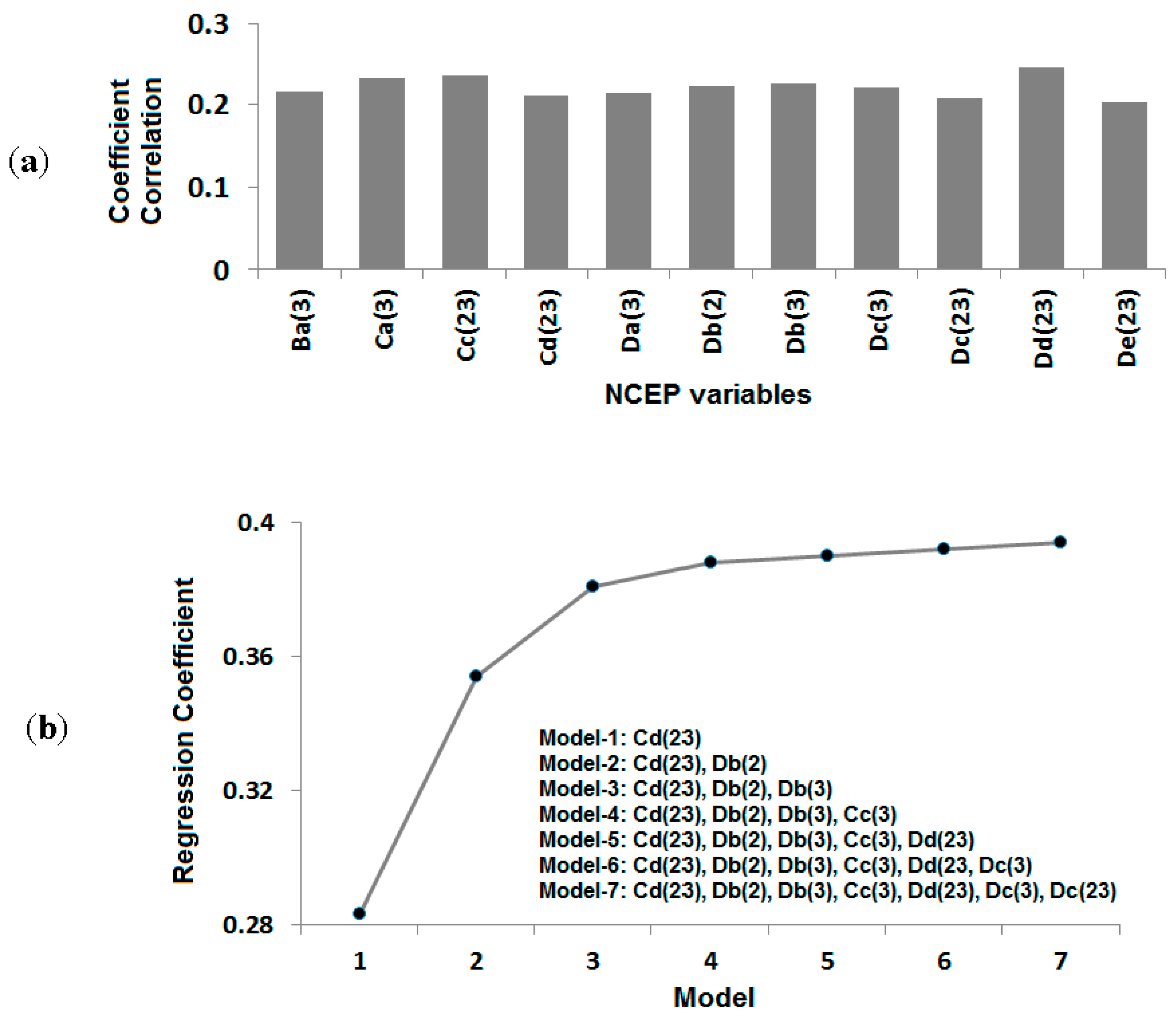
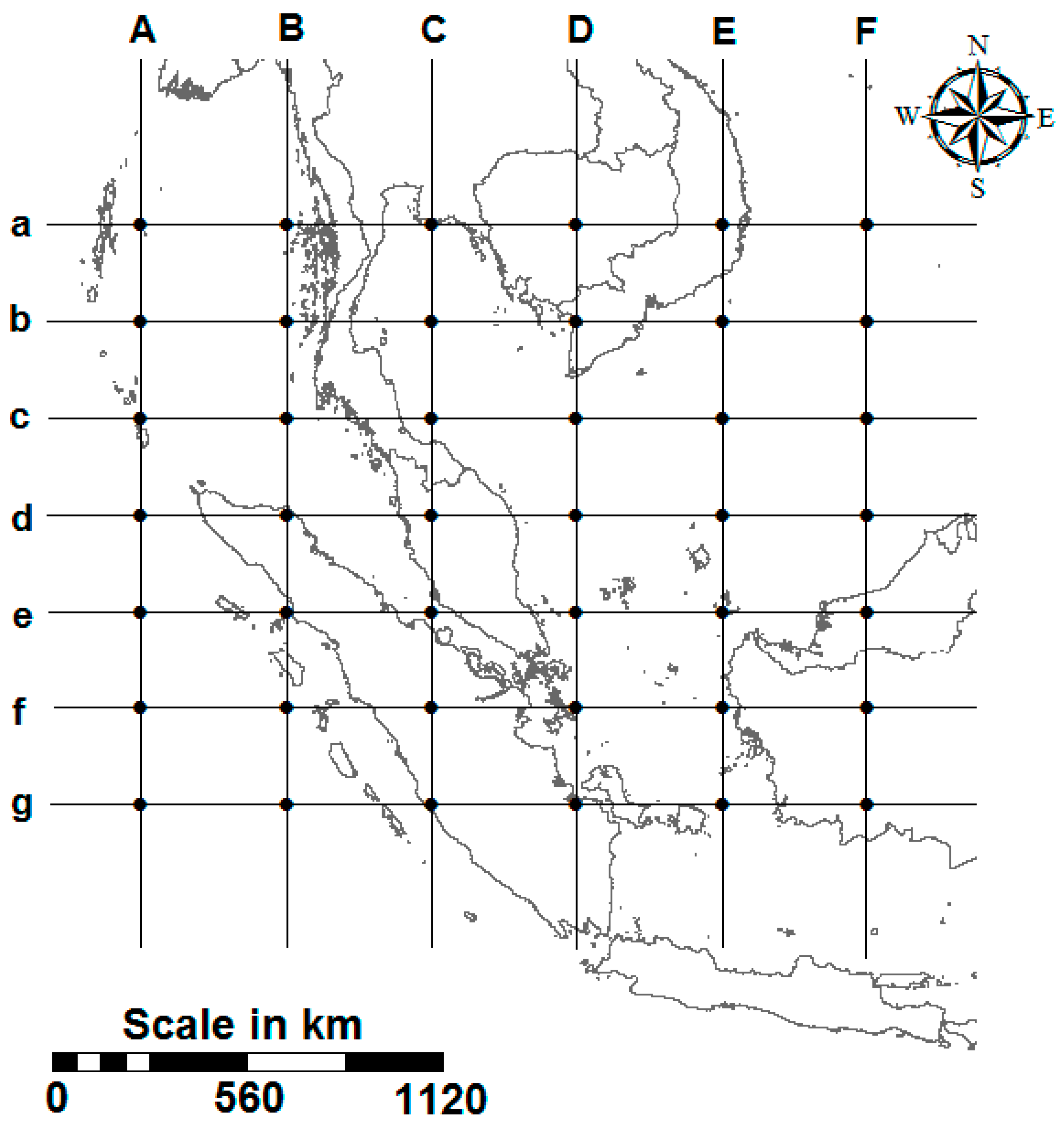
For the selection of predictors, the NCEP variables from 42 grid points surrounding the study area were individually correlated with local rainfall events. The NCEP variables from different grid points, having high correlation with heavy rainfall event at Dungun station, are shown in Figure 3a. In the figure, the capital letter in an NCEP variable name represents the column and the lower case letter represents the row of the NCEP grid point, as shown in Figure 2. The number in brackets represents the NCEP variable, as described in Table 1. Therefore, Cd(23) represents relative humidity at 500 hPa at the grid point located in column “C” and row “d”. Eleven NCEP variables from different grid points were found to have high correlation with a heavy rainfall event. These NCEP variables were used to select the final set of predictors for the downscaling using stepwise multiple regression. Stepwise multiple regression is a way of choosing predictors of a particular dependent variable on the basis of statistical criteria, such as an F-test or adjusted R-squared test. Stepwise multiple regression adds and removes predictors, in a stepwise manner, until there is no justifiable reason to add or remove more. Therefore, it allows the selection of the subset of independent variables that is the best predictor. The plot of regression coefficients between different subsets of independent variables and 90th percentile rainfall events at Dungun station is shown in Figure 3b. The figure shows that the model performance increases with the inclusion of more NCEP variables. However, it does not increase substantially after the inclusion of more variables with three independent variables, namely Cd(23), Db(2) and Db(3). Therefore, these three NCEP variables were finally chosen as predictors for the downscaling of heavy rainfall days at Dungun station.

Figure 3. (a) The NCEP variables from different grid points with good correlation with heavy rainfall events during the NE monsoon; (b) the plot of regression coefficients between different subsets of NCEP variables and heavy rainfall events at Dungun station.

Figure 3. (a) The NCEP variables from different grid points with good correlation with heavy rainfall events during the NE monsoon; (b) the plot of regression coefficients between different subsets of NCEP variables and heavy rainfall events at Dungun station.

The process produced the same set of NCEP variables for all three stations. The NCEP variables selected as predictors for different rainfall indices are given in Table 3. NCEP variables at grid points located in the NE direction have more influence on the rainfall of the study area. This is justifiable, as the rainfall in the study area is influenced by the NE monsoon.

Table 3 shows that the NCEP variables selected for downscaling rainfall indices are relative humidity at 500 and 850 hPa, surface airflow strength and surface zonal velocity. Precipitation at a location depends on the available air moisture content and flow of moist air. Relative humidity at 500 and 850 hPa represents the water vapor available in the air; surface airflow strength represents the regime of near surface air flow and surface zonal velocity on the equator cause zonal wind stress. Therefore, selection of these variables is physically plausible for rainfall downscaling. Other researchers also used those variables as predictors for rainfall downscaling in Malaysia [67,68]. It is very important to remember that the predictors used for downscaling should be reliably simulated by GCMs. The predictors selected in the present study are well simulated by many GCMs, including Hadley Centre Coupled Model, version 2 (HadCM2), Canadian Global Coupled Model, version 2 (CGCM2), etc. Therefore, these predictors have been widely used for the downscaling and projection of future rainfall [67,68,69].

Table 3. NCEP variables used to build downscaled models.

Event	Predictor	Code	Description
90th percentile rainfall event	P1	Cd(23)	Relative humidity at 500 hPa at grid point Cd
	P2	Db(2)	Surface airflow strength at grid point Db
	P3	Dc(3)	Surface zonal velocity at grid point Dc
Rainfall event	P1	Cd(23)	Relative humidity at 500 hPa at grid point Cd
	P2	Dd(24)	Relative humidity at 850 hPa at grid point Dd
	P3	Db(3)	Surface zonal velocity at grid point Db

Table 3. NCEP variables used to build downscaled models.

Event	Predictor	Code	Description
90th percentile rainfall event	P1	Cd(23)	Relative humidity at 500 hPa at grid point Cd
	P2	Db(2)	Surface airflow strength at grid point Db
	P3	Dc(3)	Surface zonal velocity at grid point Dc
Rainfall event	P1	Cd(23)	Relative humidity at 500 hPa at grid point Cd
	P2	Dd(24)	Relative humidity at 850 hPa at grid point Dd
	P3	Db(3)	Surface zonal velocity at grid point Db

3.2. Downscaling Using GP

The goal of a GP downscaling process is to produce an algebraic expression or model that best describes the daily rainfall from predictors. For this purpose, the GP algorithm works with solution candidates, which are tree structure representations of symbolic expressions. The function set used for non-terminal nodes includes +, −, ×, /, %, square root, log, as well as logical and other commonly-used trigonometric operators. As the goal is to find the extreme rainfall from NCEP variables, the terminal nodes must consist of selected NCEP variables, as well as constants. The obtained results are discussed below.

3.2.1. Downscaling Heavy Rainfall Days

A GP model for the downscaling of the days with larger than or equal to 90th percentile rainfall was developed first. The amounts of 90th percentile daily rainfall over the normal climate period (1961–1990) defined by the World Meteorological Organization [44] are 23.2, 24.6 and 25.8 mm at Besut, Dungun and Kemaman stations, respectively. GP-based logistic regression was used to decide whether 90th percentile rainfall will occur or not during a day from the NCEP variables.

The GP software (Discipulus) used in the present study performs multiple runs by default. In the present study, 100 runs were used to produce a wide range of results. Termination of each run was considered as 200 generations without any improvement in fitness function. The distribution of results from multiple GP runs includes a distributional tail of excellent solutions. The best solution is selected based on the hit rate. The highest overall hit rates were obtained in downscaling heavy rainfall days in run 52 after 652 generations at Besut station, in run 47 after 712 generations at Dungun and in run 34 after 512 generations at Kemaman. 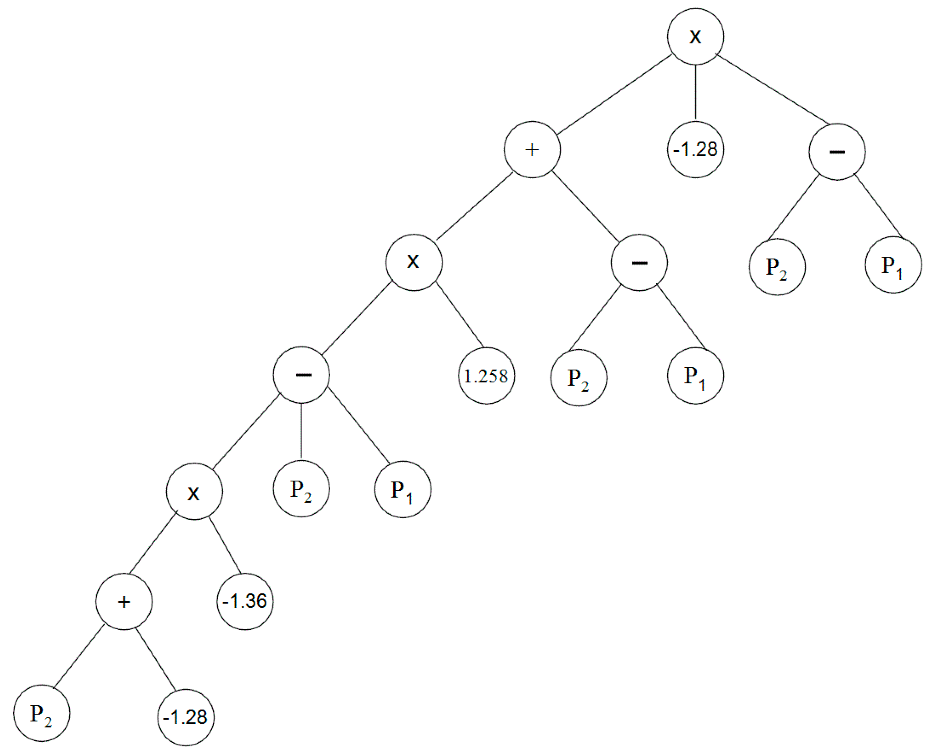The highest overall hit rates obtained at different stations is given in Table 4. It can be seen from the table that GP is able to model the 90th percentile rainfall index in 78.3%–81.1% of cases during calibration and 75.9%–78.0% of cases during validation. This means that GP-based logistic regression is successful in downscaling heavy rainfall days in more than 78.3% of cases. The best tree structure representations of symbolic expressions produced by GP in downscaling heavy rainfall days at Besut station is shown in Figure 4. The simplified equations obtained from the GP structures that can be used to downscale the number of heavy rainfall days in the vicinity of three rainfall stations is given in Table 5.

Table 4. Overall hit rates during training and validation of genetic programming (GP) models in downscaling rainfall indices.

Rainfall Indices	Station Name	Hit Rate (%)
		Training	Validation
Days with larger than or equal to 90th percentile rainfall	Besut	81.1	78.0
	Dungun	80.1	76.8
	Kemaman	78.3	75.9
Rainy days	Besut	86.1	82.0
	Dungun	84.5	80.2
	Kemaman	83.9	81.0

Table 4. Overall hit rates during training and validation of genetic programming (GP) models in downscaling rainfall indices.

Rainfall Indices	Station Name	Hit Rate (%)
		Training	Validation
Days with larger than or equal to 90th percentile rainfall	Besut	81.1	78.0
	Dungun	80.1	76.8
	Kemaman	78.3	75.9
Rainy days	Besut	86.1	82.0
	Dungun	84.5	80.2
	Kemaman	83.9	81.0

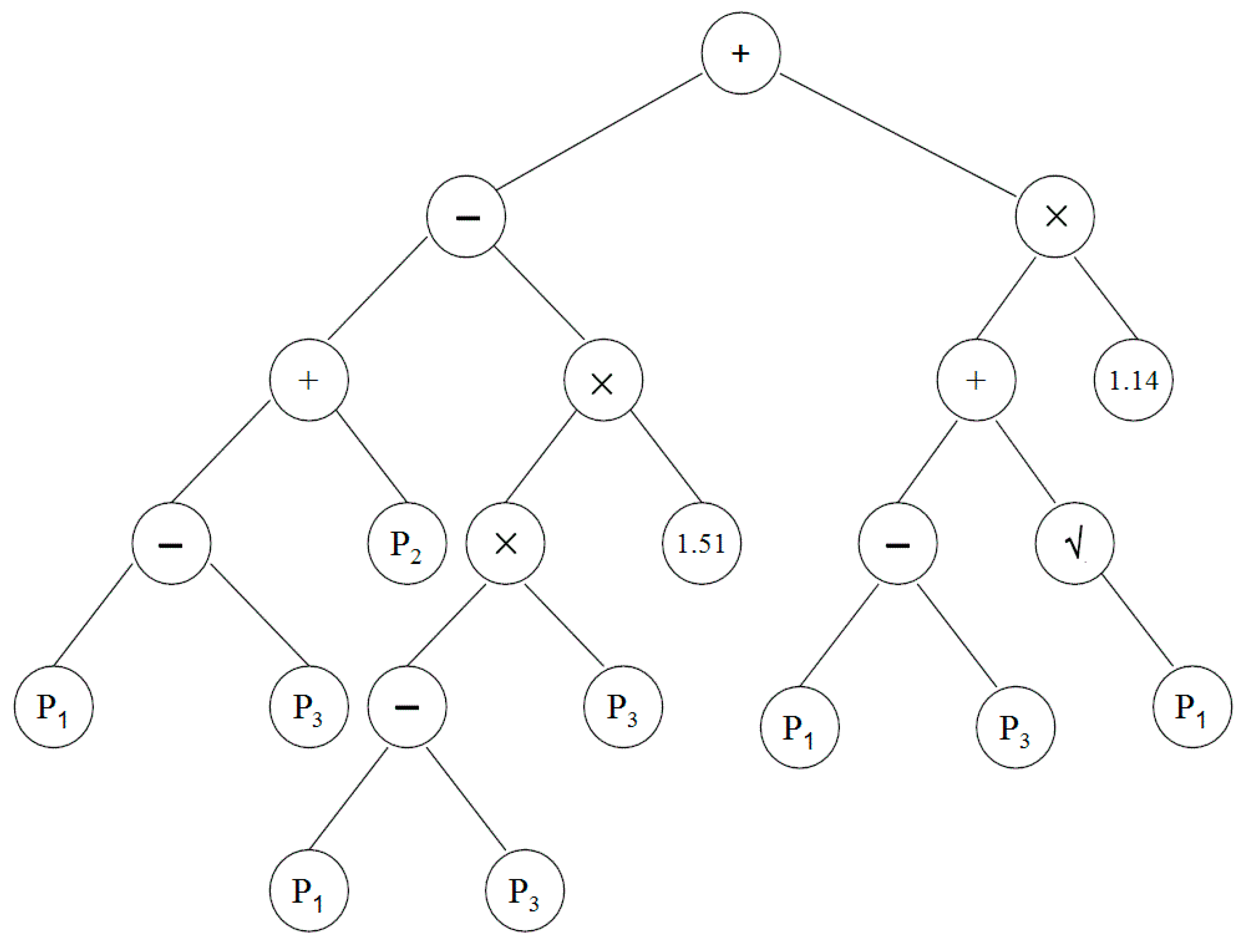
Figure 4. The tree structure representations of symbolic expressions produced by GP for heavy rainfall event downscaling at Besut (descriptions of P₁, P₂ and P₃ are given in Table 3).

Figure 4. The tree structure representations of symbolic expressions produced by GP for heavy rainfall event downscaling at Besut (descriptions of P₁, P₂ and P₃ are given in Table 3).

Table 5. The simplified equations derived by GP for the downscaling of extreme rainfall indices (descriptions of P₁, P₂ and P₃ are given in Table 3).

Rainfall Indices	Station Name	Equation
Days with larger than or equal to 90th percentile rainfall	Besut	−1.28[P2 − P1 + 1.258[P2 − P1 − 1.36[P2 + P3]]] × [P2 − P1]
	Dungun	[P2 + P1 − 2.56[P2 + P1 − 3.26[P1 + P2 + P3]]] × 1.23P2
	Kemaman	−1.11[P2 − P1 + 1.56[P2 − P1 − 1.45[P2 + P3]]] × [P2 − P1 + P3]
Rainy days	Besut	(P3 − P1 + P2) − 1.51(P3 × P2 − P1) + 1.14(P1 − P3 + sqrt(P1))
	Dungun	1.23 × (P1 + P2) − 1.26(P3 × P2 − P1) + 0.86(P1 − P2)
	Kemaman	2.34 × P2 − 2.13(P3 × 1.54 − P1) + 1.45(P1 − P3 × P1)

Table 5. The simplified equations derived by GP for the downscaling of extreme rainfall indices (descriptions of P₁, P₂ and P₃ are given in Table 3).

Rainfall Indices	Station Name	Equation
Days with larger than or equal to 90th percentile rainfall	Besut	−1.28[P2 − P1 + 1.258[P2 − P1 − 1.36[P2 + P3]]] × [P2 − P1]
	Dungun	[P2 + P1 − 2.56[P2 + P1 − 3.26[P1 + P2 + P3]]] × 1.23P2
	Kemaman	−1.11[P2 − P1 + 1.56[P2 − P1 − 1.45[P2 + P3]]] × [P2 − P1 + P3]
Rainy days	Besut	(P3 − P1 + P2) − 1.51(P3 × P2 − P1) + 1.14(P1 − P3 + sqrt(P1))
	Dungun	1.23 × (P1 + P2) − 1.26(P3 × P2 − P1) + 0.86(P1 − P2)
	Kemaman	2.34 × P2 − 2.13(P3 × 1.54 − P1) + 1.45(P1 − P3 × P1)

3.2.2. Downscaling Consecutive Wet and Dry Days

For downscaling of consecutive wet and dry days, a GP model was developed to predict whether rainfall will occur or not during a day. This produced a binary time series for the whole period, which was used to compute the consecutive wet and dry days in a year.

The GP model required different numbers of generations to give the highest overall hit rates at different stations. The best hit rates in downscaling rainy days at different stations is given in Table 4. It can be seen from the table that GP-based logistic regression was successful in downscaling rainfall days in 83.9%–86.1% of cases during calibration and 80.2%–82.0% of cases during validation. The best tree structure produced by the GP in downscaling rainy days at Besut is shown in Figure 5. The simplified equations obtained from the structures that can be used for downscaling rainy days at different stations are given in Table 5.

Figure 5. The tree structure representations of symbolic expressions produced by GP for the downscaling of rainy days at Besut (descriptions of P₁, P₂ and P₃ are given in Table 3).

Figure 5. The tree structure representations of symbolic expressions produced by GP for the downscaling of rainy days at Besut (descriptions of P₁, P₂ and P₃ are given in Table 3).

3.3. Downscaling Using ANN

A feed-forward learning-based three-layer MLP ANN developed in MATLAB was used in the present study to downscale extreme rainfall indices. The same predictors used in GP (Table 3) were also used in the ANN. Like GP, an ANN is used to decide whether rainfall will occur or not during a day from the NCEP variables. Data for the time periods 1961–1990 and 1991–2000 were used for calibration and validation of the ANN model, respectively. The ANN was run 100 times, and the obtained results from each run were stored. A termination criterion for a single run was chosen as 200 generations without improvement. The best ANN model was selected based on the hit rate. The results were then compared with those obtained using GP and the SDSM.

3.4. Downscaling Using the SDSM

The SDSM package was also used to downscale daily rainfall with the same predictors used for GP (given in Table 3). Daily rainfall data for the time periods 1961–1990 and 1991–2000 were used for calibration and validation of the SDSM, respectively. The extreme rainfall indices were then estimated from the daily rainfall downscaled by the SDSM. In the present study, extreme rainfall indices during the validation period were computed and compared with observed and GP-based downscaled results.

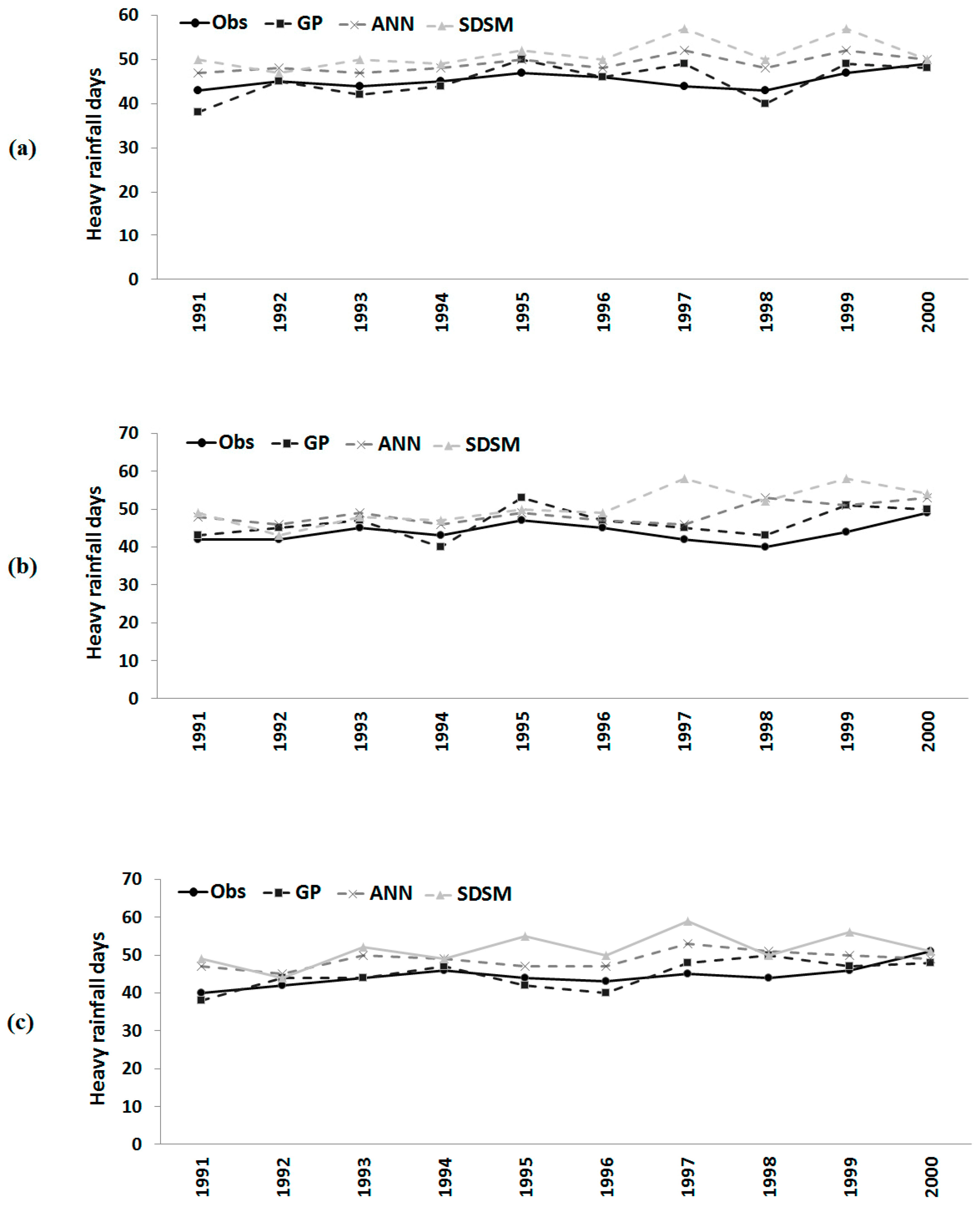
Figure 6. Observed number of heavy rainfall days and those downscaled by GP, the ANN and the statistical downscaling model (SDSM) during model validation at: (a) Besut; (b) Dungun; and (c) Kemaman.

Figure 6. Observed number of heavy rainfall days and those downscaled by GP, the ANN and the statistical downscaling model (SDSM) during model validation at: (a) Besut; (b) Dungun; and (c) Kemaman.

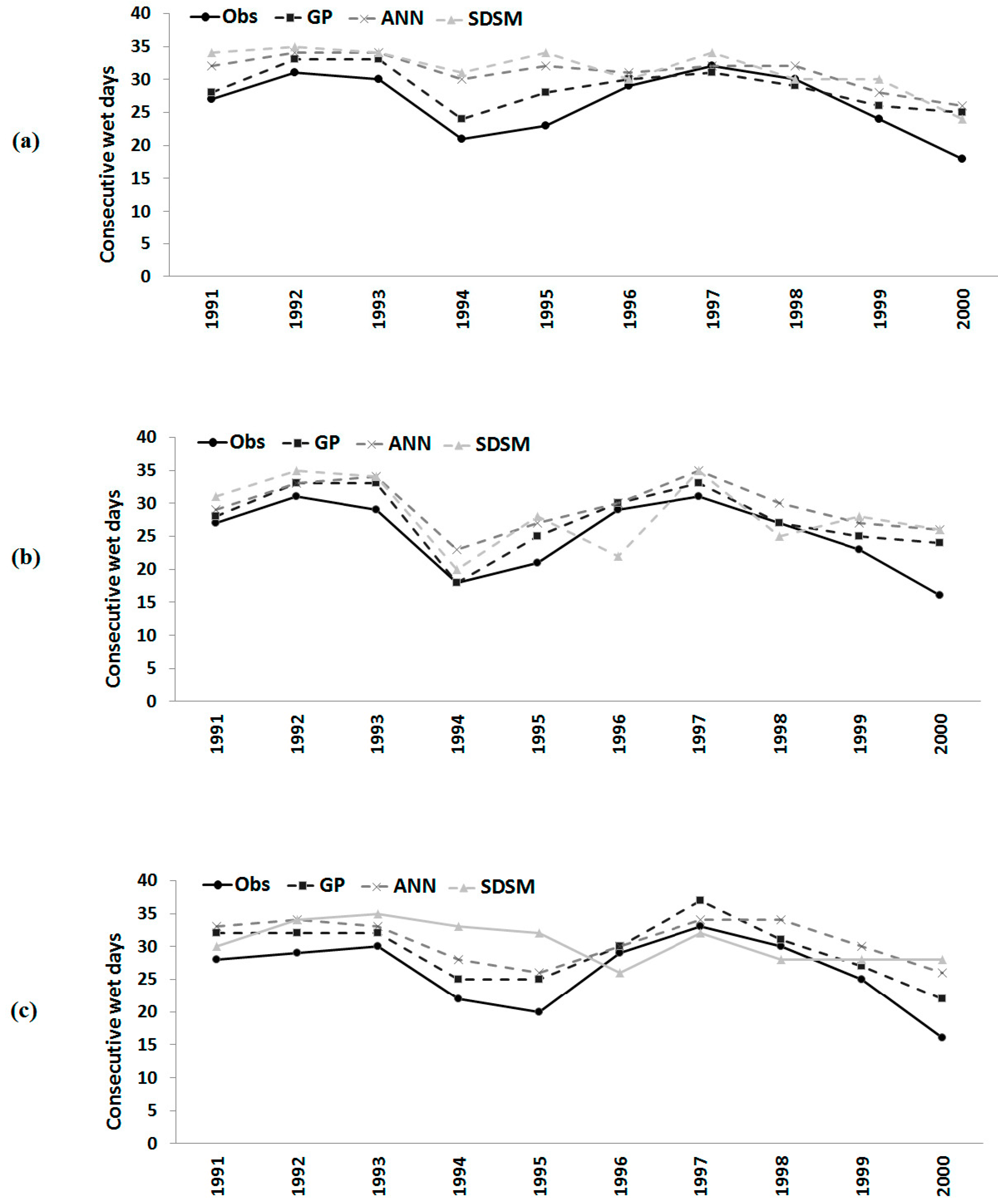
Figure 7. Observed number of consecutive wet days and those downscaled by GP, the ANN and the SDSM during model validation at: (a) Besut; (b) Dungun; and (c) Kemaman.

Figure 7. Observed number of consecutive wet days and those downscaled by GP, the ANN and the SDSM during model validation at: (a) Besut; (b) Dungun; and (c) Kemaman.

3.5. Comparison of Results

Comparisons of observed and downscaled heavy rainfall days during monsoon, as well as consecutive wet days and consecutive dry days in a year over the model validation period (1991–2000) are shown in Figure 6, Figure 7 and Figure 8, respectively. It can be seen in Figure 6 that all of the methods estimated the number of heavy rainfall days successfully over the evaluation period. However, the downscaled output from GP is closer to the observed values compared to those estimated by the ANN and the SDSM. In most of the years, both the ANN model and SDSM overestimated the number of heavy rainfall days. Compared to the ANN, the SDSM overestimated heavy rainfall days more often. On the other hand, GP underestimated the number of days in certain years, but the estimated GP values were found to be very close to observed values in almost all of the years and at all of the stations. The root mean squared error (RMSE) and correlation coefficient (expressed as r²) between observed and downscaled values during validation are given in Table 6. The table shows that the errors in estimation of the number of heavy rainfall days by GP are always significantly less compared to ANN and SDSM estimations. The correlation coefficient between observed values and GP downscaled values during the validation period was also found to be higher compared to ANN and SDSM downscaling.

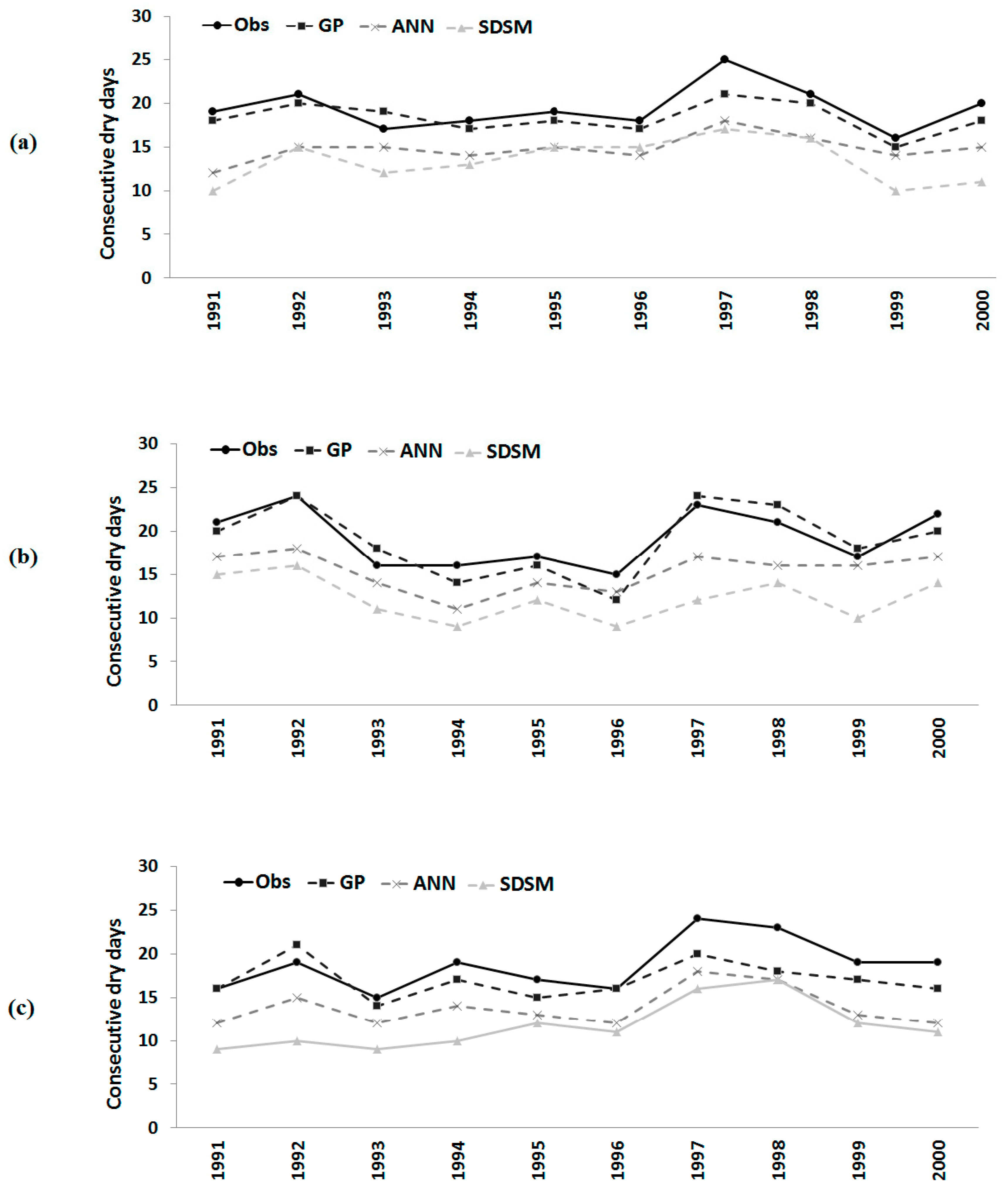
Figure 8. Observed number of consecutive dry days and those downscaled by GP, the ANN and the SDSM during model validation at (a) Besut; (b) Dungun; and (c) Kemaman.

Figure 8. Observed number of consecutive dry days and those downscaled by GP, the ANN and the SDSM during model validation at (a) Besut; (b) Dungun; and (c) Kemaman.

Similar results were obtained for consecutive wet days and consecutive dry days in a year. It can be seen from Figure 7 that the number of consecutive wet days in a year was overestimated by the ANN model and SDSM in most of the years at all three stations during the validation period. GP also overestimated the number of consecutive wet days in certain years. However, GP downscaled values are found to be closer to observed values compared to those downscaled by the ANN and SDSM at all of the stations. Table 6 shows that the errors in the number of consecutive wet days in a year estimated by GP is always significantly less compared to ANN and SDSM estimations. The correlation coefficient between observed and GP downscaled values during the validation period was also found to be higher.

Errors in GP downscaling of the number of consecutive dry days in a year were found to be similar to those in the estimations of the other two extreme indices. It can be seen from Figure 8 that the downscaled number of consecutive dry days in a year by GP, the ANN and SDSM is less than the observed number of days in most of the years at all three stations. However, GP downscaled values are still found to be closer compared to those downscaled by the ANN and SDSM.

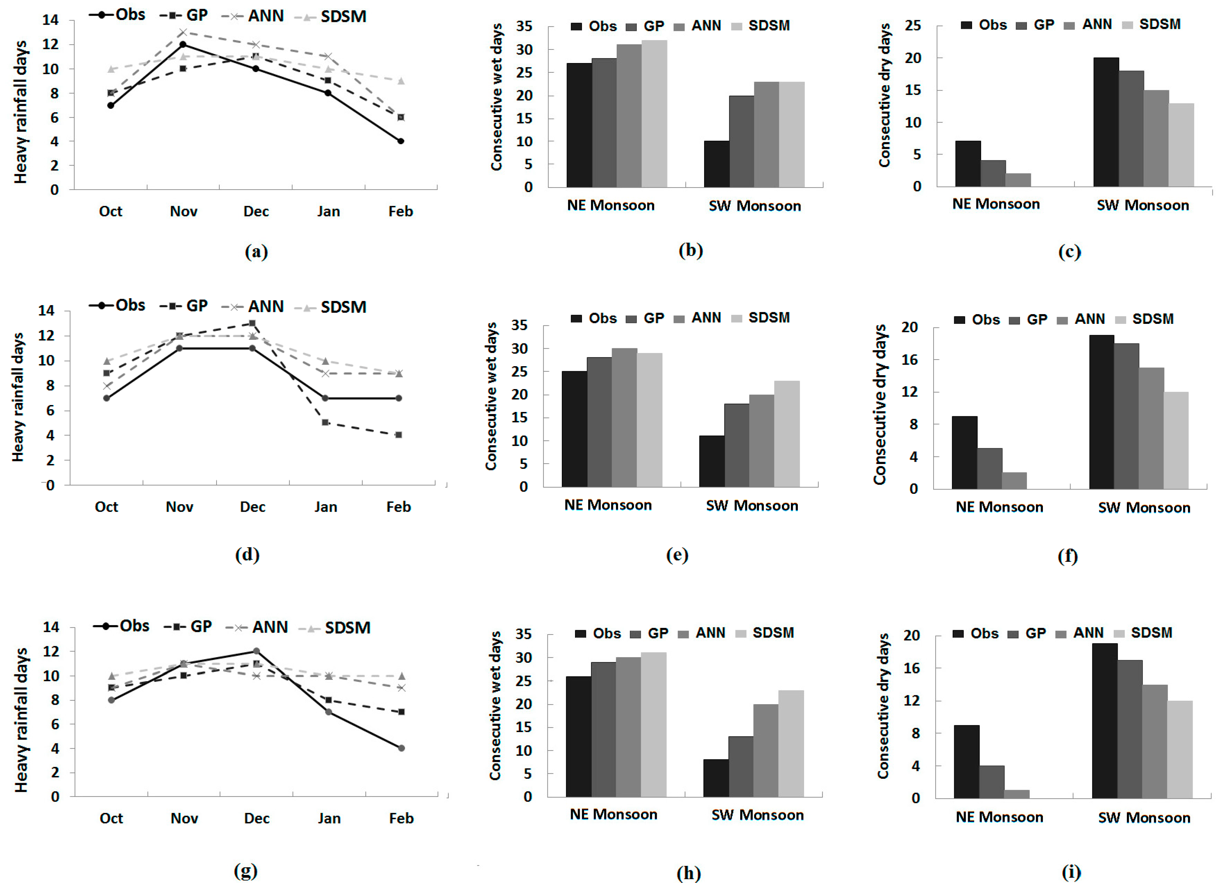
Comparison of observed and downscaled heavy rainfall days during different months of the NE monsoon, as well as continuous wet days and continuous dry days during NE and SW monsoons at different stations during model validation is shown in Figure 9. It can be seen from Figure 9 that seasonal or monthly variations in extreme rainfall indices are well reconstructed by GP compared to those by the ANN and SDSM. In the case of heavy rainfall days, the SDSM was found to downscale almost to the same number in all of the NE monsoon months. The ANN is able to show some variation in the number of heavy rainfall days, but not like GP. It can also be noted from the values in Figure 9 that all of the methods overestimated the number of heavy rainfall days in most of the months. Still, the values estimated by GP are closer to the observed values compared to those estimated by the ANN and SDSM. The RMSEs between the observed and estimated number of heavy rainfall days using different methods during model validation are given in Table 7. The table shows that the error in the estimation of the number of heavy rainfall days by GP is always less compared to the ANN and SDSM.

Table 6. The RMSEs and correlation coefficients (r²) between observed and downscaled extreme indices estimated by GP, the ANN and the SDSM during model validation.

Indices	Station	GP		ANN		SDSM
		RMSE	r2	RMSE	r2	RMSE	r2
90th percentile rainfall days	Besut	1.08	0.75	1.31	0.58	2.16	0.43
	Dungun	1.14	0.73	1.83	0.58	2.69	0.41
	Kemaman	1.13	0.67	1.62	0.61	2.57	0.51
Consecutive wet days	Besut	1.02	0.88	1.73	0.80	1.95	0.65
	Dungun	1.05	0.89	1.54	0.83	1.74	0.61
	Kemaman	1.10	0.96	1.66	0.92	2.20	0.46
Consecutive dry days	Besut	1.06	0.83	1.55	0.73	1.99	0.67
	Dungun	1.04	0.91	1.65	0.87	2.28	0.85
	Kemaman	1.23	0.82	1.60	0.82	2.26	0.77

Table 6. The RMSEs and correlation coefficients (r²) between observed and downscaled extreme indices estimated by GP, the ANN and the SDSM during model validation.

Indices	Station	GP		ANN		SDSM
		RMSE	r2	RMSE	r2	RMSE	r2
90th percentile rainfall days	Besut	1.08	0.75	1.31	0.58	2.16	0.43
	Dungun	1.14	0.73	1.83	0.58	2.69	0.41
	Kemaman	1.13	0.67	1.62	0.61	2.57	0.51
Consecutive wet days	Besut	1.02	0.88	1.73	0.80	1.95	0.65
	Dungun	1.05	0.89	1.54	0.83	1.74	0.61
	Kemaman	1.10	0.96	1.66	0.92	2.20	0.46
Consecutive dry days	Besut	1.06	0.83	1.55	0.73	1.99	0.67
	Dungun	1.04	0.91	1.65	0.87	2.28	0.85
	Kemaman	1.23	0.82	1.60	0.82	2.26	0.77

Figure 9. Monthly/seasonal distribution of: (a) heavy rainfall days, (b) consecutive wet days and (c) consecutive dry days at Besut; (d) heavy rainfall days; (e) consecutive wet days and (f) consecutive dry days at Dungun; and (g) heavy rainfall days, (h) consecutive wet days and (i) consecutive dry days at Kemaman.

Figure 9. Monthly/seasonal distribution of: (a) heavy rainfall days, (b) consecutive wet days and (c) consecutive dry days at Besut; (d) heavy rainfall days; (e) consecutive wet days and (f) consecutive dry days at Dungun; and (g) heavy rainfall days, (h) consecutive wet days and (i) consecutive dry days at Kemaman.

Table 7. The RMSE in downscaled seasonal extreme indices using GP, the ANN and the SDSM during model validation.

Indices	Station	GP	ANN	SDSM
90th percentile rainfall days	Besut	1.66	2.18	3.16
	Dungun	1.68	2.35	2.45
	Kemaman	1.80	3.12	3.54
Consecutive wet days	Besut	5.02	6.80	6.96
	Dungun	3.81	5.15	6.32
	Kemaman	2.92	6.96	7.91
Consecutive dry days	Besut	1.80	3.54	4.95
	Dungun	2.06	4.03	5.70
	Kemaman	2.69	4.72	5.70

Table 7. The RMSE in downscaled seasonal extreme indices using GP, the ANN and the SDSM during model validation.

Indices	Station	GP	ANN	SDSM
90th percentile rainfall days	Besut	1.66	2.18	3.16
	Dungun	1.68	2.35	2.45
	Kemaman	1.80	3.12	3.54
Consecutive wet days	Besut	5.02	6.80	6.96
	Dungun	3.81	5.15	6.32
	Kemaman	2.92	6.96	7.91
Consecutive dry days	Besut	1.80	3.54	4.95
	Dungun	2.06	4.03	5.70
	Kemaman	2.69	4.72	5.70

The number of consecutive wet days in two major seasons (SW monsoon and NE monsoon) was overestimated by the ANN and SDSM during the validation period at all three stations (Figure 9). GP also overestimated the number of consecutive wet days, but GP downscaled values were found to be closer to observed values compared to those downscaled by the ANN and SDSM in both of the seasons and at all of the stations. Table 7 shows that the errors in estimation of seasonal consecutive wet spells estimated by GP are always less compared to those estimated by the ANN and SDSM. Errors in the downscaling number of seasonal dry spells are also found to be less for GP. It can be seen from Figure 9 that downscaled lengths of seasonal dry spells estimated by GP, the ANN and the SDSM are lower than the observed number of consecutive dry days in both seasons at all of the stations. However, GP downscaled values were still found to be closer compared to those downscaled by the ANN and SDSM.

4. Conclusions

Downscaling daily rainfall is an extremely difficult task, as the relations between predictors and predictands are often difficult to map. This is especially true for Malaysia, where relations between local rainfall and ocean-atmospheric circulation parameters are not clearly understood. The application of GP shows that extreme rainfall indices in a tropical area, like the east coast of Peninsular Malaysia, can be downscaled with reasonable accuracy. It is expected that the GP-based methodology proposed in the present study can be used as a reliable tool for the projection of extreme rainfall indices at the local and regional scale, where climate projection under different climate change scenarios is important.

It should be noted that extreme weather phenomena often occur at small scales; thus, coarse resolution models may not always be able to simulate extreme rainfall events accurately. In projecting future climates using downscaling models, it should be remembered that GCMs designed with a single run for long-term climate projection are apparently not dependent on the initial model conditions, as they are soon destroyed after a short period of simulation. These models, as a result, tend to diagnose tendencies of future climate states rather than precise predictions of whether particular events are likely to occur [70]. Downscaled models contain considerable uncertainties, and quantification of uncertainty for the outputs of downscaling models is very important. Studies can be carried out in the future to quantify the uncertainty in GP-based models in the downscaling of extreme rainfall indices on the east coast of Peninsular Malaysia.