Article

Satellite-Observed Transport of Dust to the East China Sea and the North Pacific Subtropical Gyre: Contribution of Dust to the Increase in Chlorophyll during Spring 2010

1
State Key Laboratory of Numerical Modeling for Atmospheric Sciences and Geophysical Fluid Dynamics, Institute of Atmospheric Physics, Chinese Academy of Sciences, Beijing 100029, China
2
State Key Laboratory of Satellite Ocean Environment Dynamics, Second Institute of Oceanography, State Oceanic Administration, Hangzhou 310012, China
3
Key Laboratory of Regional Climate-Environment for Temperate East Asia, Institute of Atmospheric Physics, Chinese Academy of Sciences, Beijing 100029, China
4
Key Laboratory of Marine Environmental Science and Ecology, Ocean University of China, Ministry of Education of China, Qingdao 266010, China
5
State Key Laboratory of Severe Weather/Institute of Atmospheric Composition, Chinese Academy of Meteorological Sciences, Beijing 100081, China
6
Key Laboratory of Cloud-Precipitation Physics and Severe Storms, Institute of Atmospheric Physics, Chinese Academy of Sciences, Beijing 100029, China
*
Authors to whom correspondence should be addressed.
Atmosphere 2016, 7(11), 152; https://doi.org/10.3390/atmos7110152
Submission received: 27 September 2016 / Revised: 15 November 2016 / Accepted: 17 November 2016 / Published: 23 November 2016

Abstract

:
Multiple data sets were combined to investigate five dust storm events over East Asia in spring 2010 and their impacts on chlorophyll in the East China Sea (ECS) and the North Pacific Subtropical Gyre (NPSG). Satellite-observed column aerosol images were able to show the spatial distribution of the transport of dust from the source regions to the two seas for some of the dust storm events. The CALIPSO satellite showed the vertical structure of dust aerosol for a greater number of dust storm events, including some weak events. This was confirmed by simulations of dust deposition and backward trajectories traced to dust source regions. The simulated dust deposition flux for five dust storms ranged from 13.0 to 145.6 mg·m−2·d−1 in the ECS and from 0.6 to 5.5 mg·m−2·d−1 in the NPSG, suggesting that the highest deposition was about one order of magnitude higher than the lowest. The estimated nutrients from dust showed that dust containing iron had the greatest effect on phytoplankton growth in both seas; the iron deposited by one dust storm event accounted for at least 5% of growth and satisfied the increase in demand required for chlorophyll a concentration.

1. Introduction

East Asian dust storms (defined here as dust storms produced in China, Mongolia, Kazakhstan and the south of the Tibetan Plateau) have three major sources: (1) deserts in Mongolia; (2) deserts in western China, including the Taklimakan Desert; and (3) high dust emission areas in northern China, including the Badain Jaran Desert, the Tengger Desert and the Ulan Buh Desert [1]. The deserts in Mongolia and northern China are also referred to as the Gobi Desert. Dust storms are classified into five categories according to the horizontal visibility and the intensity of the storm: super-severe dust storms > severe dust storms > dust storms > blowing dust > floating dust [2]. The horizontal visibility in the above five storms is <50 m, <500 m, <1 km, 1–10 km (mean wind speed >3 m·s−1), and <10 km (no wind or mean wind speed ≤3 m·s−1), respectively. In spring 2010, satellite observations, surface measurements of PM10 concentrations and various models were used to observe and simulate a severe dust storm episode from 19 to 23 March [3,4,5,6]. The dust storm occurred in the west and north of China and affected large areas from the source to the western Pacific [3,4,5,6]. A very high aerosol plume was identified across the East China Sea (ECS) on 20–21 March 2010 by both satellite observations and models [3,4,6]. However, the transport pathways of Asian dust events from the source regions to the downwind marginal seas and the North Pacific Ocean are still unclear as a result of a lack of large-scale, long-term observations.
The impacts of atmospheric deposition on the ocean have received increasing attention since the development of the “iron hypothesis”—that is, the suggestion that iron-containing soil dust deposited in the oceans may stimulate marine biological productivity and reduce atmospheric concentrations of carbon dioxide [5,6,7,8,9,10,11,12,13,14,15,16]. Inputs of eolian dust containing nutrients such as iron, nitrogen and phosphorus to the oceans can affect the ocean biogeochemistry and result in feedback effects on both climate and dust production [10]. Both macronutrients (e.g., nitrogen and phosphorus) and micronutrients (e.g., iron) have attracted attention because they play important roles in marine biological productivity [13,17,18,19]. Cruise observations have found that biological activity can be influenced by atmospheric deposition, especially sporadic dust storm events (e.g., Bishop et al. [20]; Shi et al. [16]).
Many studies have proposed a correlation between the deposition of dust and biological activity and phytoplankton bloom events in the western North Pacific, the Sea of Japan (also known as the East Sea) and the coastal seas of China [11,12,21,22]. Tan et al. [22] reported a significant positive correlation between the chlorophyll a concentration from coastal seas to the open Pacific Ocean and the frequency of dust storms observed in Mainland China over an 11-year period. However, there have only been a few studies of the direct link between dust deposition and phytoplankton blooms during dust storm events. There is a time delay for the response of phytoplankton to dust deposition because both short-term (minutes to hours) and long-term (days to weeks) aerosol dissolution processes take place within the ocean [23]. Both satellite observations and onboard measurements from ships have found that dust events may have increased the concentrations of chlorophyll a in the Yellow Sea [6,16]. Wang et al. [5] demonstrated that the biogeochemistry of the northern South China Sea, a coastal sea, responds significantly to the atmospheric input of Asian dust. Their results suggested that dust events could double the background chlorophyll a concentration in spring.
There have been few reported studies comparing dust deposition and its impact on phytoplankton growth in marginal seas and open oceans, especially studies comparing different seas. The transport pathways of dust aerosols from the source regions to the sea require further study. How much dust is deposited into the sea during each dust storm event and the differences between weak and severe dust storm events is also unknown. The contribution of dust deposition to phytoplankton growth in marginal seas and open oceans also needs further study. To compare the impact of dust deposition on marginal seas and the open ocean, this study investigated phytoplankton growth after the deposition of several dust storm events in spring 2010 in the ECS (a marginal sea) and the North Pacific Subtropical Gyre (NPSG, open ocean). The study used a variety of datasets, including the satellite-observed column and vertical aerosol properties, simulated dust deposition, backward trajectories and satellite-observed ocean color data.

2. Data and Methods

In spring 2010, the Sand Dust Weather Almanac reported several dust storms, including one severe dust storm [24]. A severe dust storm occurred from 19 to 22 March 2010 in western and northern China. Many studies have been published on this severe dust storm event [3,4,6,25], but none on other dust storm events in spring 2010. We investigated five dust storms affecting the ECS and the NPSG using satellite-based instruments. A combination of the satellite-observed aerosol properties, backward trajectories, simulated dust deposition and ocean color data were used to track the transport of the dust storm and to investigate the impact of dust deposition on phytoplankton growth in the ECS and NPSG. The satellite-observed vertical structure of dust aerosol was used to identify the date on which the dust storms passed over the seas. The satellite-observed column aerosol image could illustrate the spatial distribution of the aerosols during dust storms and could be a consistency check on the passage date identified by vertical structure. Backward trajectories were used for validation for satellite results. Simulated dust deposition was used to estimate the deposition of nutrients into the seas and could also validate satellite results. The satellite-observed ocean color data were needed to investigate the link between dust deposition and phytoplankton growth.

2.1. Vertical Profile and Column Properties of Satellite-Observed Aerosols

The Cloud-Aerosol Lidar with Orthogonal Polarization (CALIOP) instrument onboard the Cloud-Aerosol Lidar and Infrared Pathfinder Satellite Observations (CALIPSO) satellite has vertically resolved Level 2, Version 3 aerosol profiles products [26]. The aerosol extinction coefficient at 532 nm and the type of aerosol were used to identify the transport of dust. These properties are crucial in understanding the vertical distribution of dust particles and distinguishing dust from other aerosols. These data have a 5 km horizontal resolution. The vertical resolution for the aerosol types was 30 m below 8.2 km, 60 m between 8.2 and 20.2 km and 180 m above 20.2 km; the vertical resolution for the extinction coefficient below 8.2 km was 60 m. It was identified that the pure dust CALIOP classifications may be polluted dust due to different particle depolarization ratios [27,28]. The low dust Lidar ratio (LR) of 40 sr used in CALIOP algorithm could produce an underestimation of 532 nm extinction coefficient by 25%–35% over the Sahara and Europe, where the measured mean LR was around 51–58 sr [27,28], but 40 sr LR applied well over the Middle East [27]. Reported LR at 532 nm for Asian dust was 43 sr [29] or 51 sr (range 42–55 sr) [30], which suggested CALIOP extinction may be appropriate or underestimated for Asian dust. Uno et al. [31] indicated that CALIOP dust extinction showed a good agreement with model simulations near the Asian dust source regions.
The spatial distribution of the aerosols during dust storm events was investigated by the UV aerosol index product from the Ozone Monitoring Instrument onboard the Aura satellite and the aerosol optical depth (AOD) product from the Moderate Resolution Imaging Spectroradiometer (MODIS) onboard the Aqua satellite. Aerosol index was used to detect the UV-absorbing aerosols, such as dust and carbonaceous aerosols. Aerosols that absorb in the UV are the most important source of positive aerosol index values [32]. Aerosol index > 0.7 or 1.0 was used to identify all major global dust sources [33]. Both datasets provide useful information on the daily spatial distribution of dust clouds [6,25,33] and have a spatial resolution of 1° × 1°. The daily AOD at 550 nm data were from the Collection 006 MYD08_D3 product.

2.2. Backward Trajectory Model and Meteorological Data

The Hybrid Single Particle Lagrangian Integrated Trajectory (HYSPLIT) backward trajectory model [34] was performed to identify the source region and corresponding transport path of the dust storm affecting the ECS and the NPSG. Meteorological data were from the National Centers for Environmental Prediction/National Center for Atmospheric Research (NCEP/NCAR) global reanalysis dataset. The data were on a latitude–longitude grid with a resolution of 2.5° × 2.5°. The internal scaling height of HYSPLIT was 25 km. An air parcel at the altitude where the dust aerosols were located was traced backward and the dust layer was identified from the CALIOP vertical profiles over the research seas.

2.3. Dust Transport Model

Simulated dust deposition data (including dry and wet deposition) were used to estimate the direct link between the dust storm and phytoplankton growth. The Regional Air Quality Model System (RAQMS) numerical model driven by the fifth-generation Penn State/NCAR Mesoscale Model [35] was used to simulate the key processes of the major chemical components in the atmosphere, including emission, advection, diffusion, dry and wet deposition, aqueous and heterogeneous chemistry and cloud formation [3,36,37,38]. Soil dust aerosols were represented by a sized-segregated dust module and were divided into ten size bins ranging from 0.43 to 42 μm. The model domain covered 75.5° E to 160.5° W and 10.5°–50.5° N with a spatial resolution of 0.5° × 0.5°, including dust source regions in East Asia and the ECS and NPSG. Comparisons with the in situ PM10 concentration observed in China, the extinction coefficient of dust measured by Lidar in Japan and the aerosol index retrieved by satellite have previously indicated [3] that the model can accurately predict the outbreak, development, transport and depletion processes of dust storms over China and downwind regions. The details of this model have been described by Han [36] and Li et al. [3].
The dust storms related to this study occurred from March to May in 2010. Li et al. [3] only validated modeled PM10 concentration in March 2010, thus we included the comparison of April and May. Four cities near dust storm source regions (Hohhot, Urumqi, Lanzhou, and Xi’an) and one coastal city of the ECS (Shanghai) were chosen for comparison (Table 1). Significant (p < 0.05) correlations between modeled and observed PM10 concentration (R = 0.49–0.85) suggested that the RAQMS model not only performed well in March [3] but also in the whole spring.

2.4. Satellite-Observed Ocean Color and Climatological Ocean Nutrients

The chlorophyll a concentrations recorded by satellite remote sensing data were used to investigate phytoplankton growth and bloom events in the ECS and NPSG. Sea surface temperature (SST) and photosynthetic available radiation (PAR) data were applied to check the temperature and light levels required for phytoplankton growth. The chlorophyll a concentration was taken as the mean of the SeaWiFS and Aqua MODIS product to reduce the missing regions in each dataset. The SST and PAR were Aqua MODIS products. All these data were Level 3 Standard Mapped Image products with a 9 km × 9 km spatial resolution and were obtained from the Ocean Color website supported by the Ocean Biology Processing Group at NASA’s Goddard Space Flight Center.
The initiation, growth and decay of phytoplankton blooms can be estimated from the chlorophyll a concentration recorded by satellite data after the removal of outliers. Coastal seas with a depth <70 m in the ECS and <1000 m in the NPSG were excluded to minimize the influence from rivers and inland sources of nutrients. Following the method of Calil et al. [15], outliers with images <100 pixels after the removal of values less than the springtime climatological mean in the ECS (0.5 mg·m−3) or the background value in the NPSG (0.08 mg·m−3) were also excluded.
The nutrients data from the World Ocean Atlas (WOA) (2009) were applied to analyze the nutrient structure in the ECS and NPSG. The WOA is a data product of the Ocean Climate Laboratory of the National Oceanographic Data Center. Bathymetry and global relief data from the National Oceanographic Data Center were used to exclude the coastal regions to reduce the effect of terrestrial processes.

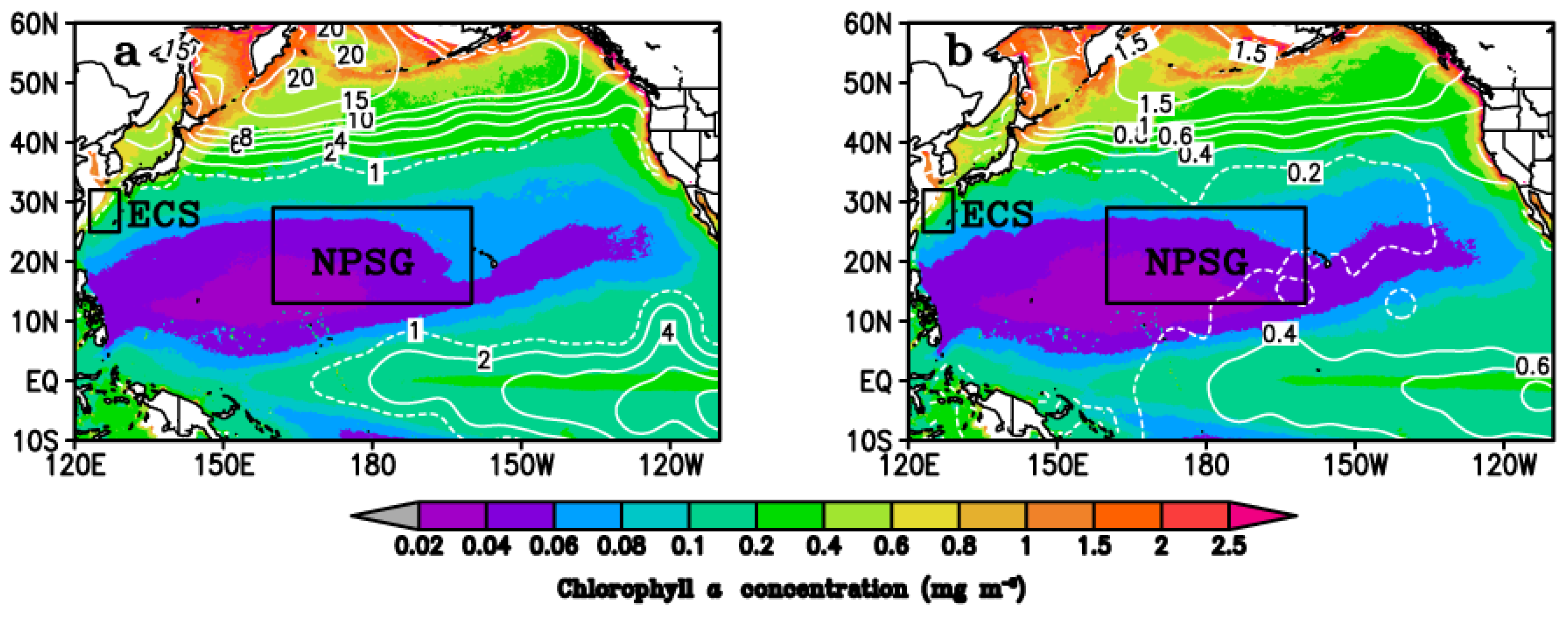
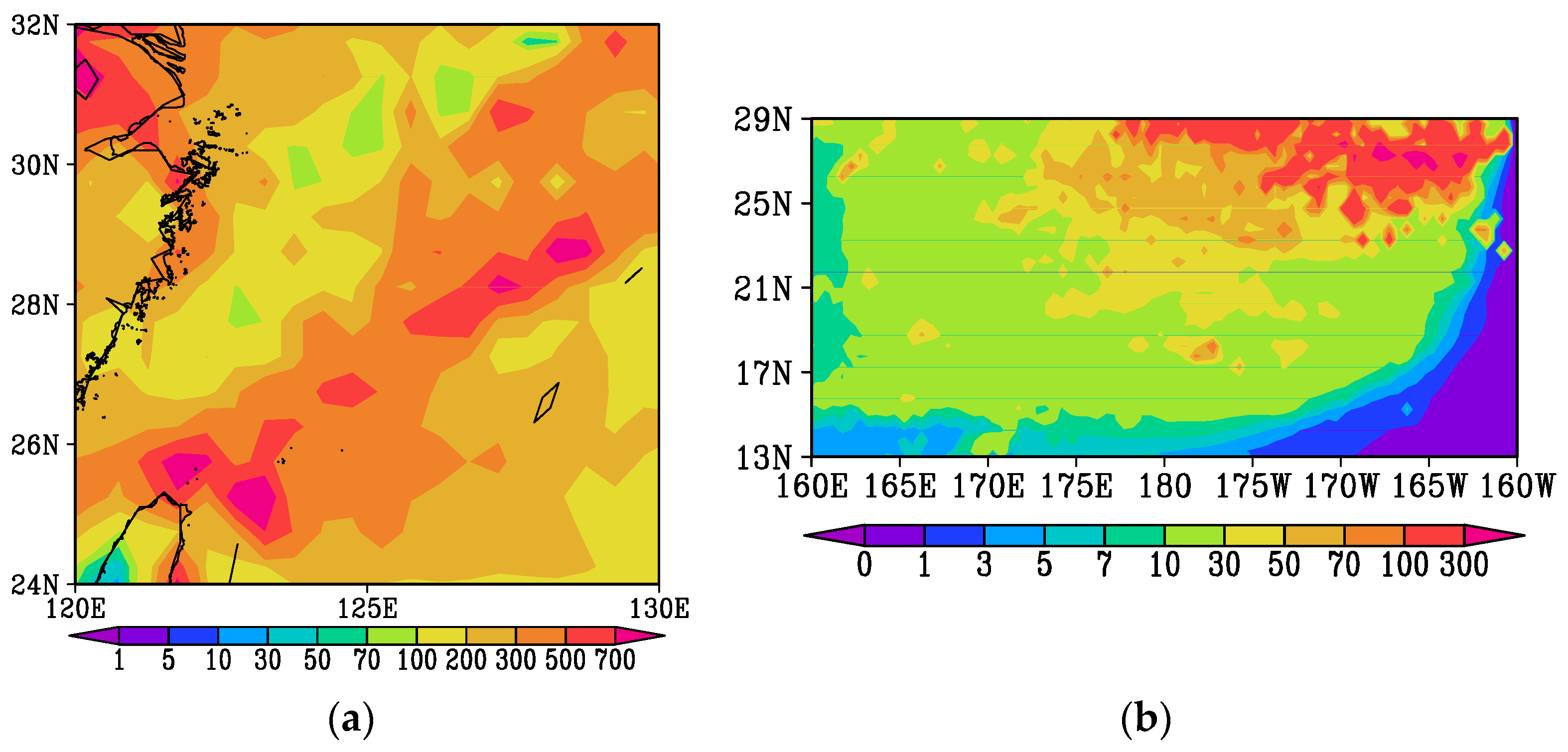
3. Environmental Background in the ECS and NPSG

The ECS was selected in the region (123°–129°E, 25°–32°N) (Figure 1). The Yangtze River runoff and the southward flow of the Min-Zhe coastal current result in high nutrient concentrations on the inner shelf of the ECS [39,40,41]. Gong et al. [39] showed that the northwestern part of the shelf in the ECS has a nutrient-enriched regime. This region has a depth <70 m and therefore the coastal seas with depths <70 m were excluded to minimize the influence of the river and inland areas on the ECS. In the outer shelf of the ECS, the Kuroshio water mass flows northeastward along the continental shelf margin within isobaths of around 200–1000 m and then turns to the east at about 30° N. It then flows eastward into the Pacific Ocean through the Tokara Straits. The Kuroshio water mass is characterized by high temperatures (>20.55 °C), high salinity (>34.5 psu) and low concentrations of particles and dissolved nutrients [40,41]. In the northwestern part of the research area, the mixed warm water of the Taiwan Warm Current is characterized by a sub-maximum salinity and sub-maximum temperature [40]. The WOA (2009) data showed that the annual mean concentrations of nitrate (Figure 1a) and phosphate (Figure 1b) at the surface in the ECS were 0.74 and 0.13 μmol·L−1, respectively. Cruise measurements indicated that the chlorophyll a concentration in the outer shelf of the ECS showed a seasonal variation, with the highest value in spring and the lowest value in summer [39]. The SeaWiFS (Figure 1a) and MODIS (Figure 1b) climatological annual chlorophyll a concentrations in the research area were 0.32 and 0.30 mg·m−3, respectively. Compared with the Sea of Japan [22] and the northern Arabian Sea (monthly mean chlorophyll a concentration >1.0 mg·m−3) [42], this area can be considered as a middle-level nutrient region. Based on the Redfield ratio (C:N:P 106:16:1), the ecosystem may be limited by phosphate in the northwestern region close to the Yangtze River and by nitrogen in other regions [43,44]. Atmospheric depositions are an external source of material to the oceans and have an important role in determining the biogeochemistry of nutrient species (including nitrogen and phosphorus) in the ECS [45]. Bioavailable micronutrients, such as iron from mineral dust, are also important.
The NPSG is characterized as a typical low nutrient–low chlorophyll region [46]. The NPSG is induced by the strong vertical stratification generated by wind-driven anticyclonic circulation in the upper 50 m of the ocean, which insulates the upper nutrient-limited layer from the nutrient-rich deeper waters and restricts exchange with adjacent current systems [15,46]. The climatological annual mean surface concentrations of nitrate, phosphate and chlorophyll a concentration for the region (160°E to 160°W, 13°–29°N) (Figure 1a,b) were 0.14 μmol·L−1, 0.13 μmol·L−1 and 0.051 (SeaWiFS) or 0.047 (MODIS) mg·m−3, respectively. In the eastern portion of the NPSG (east of 160° W), blooms were defined as regions with chlorophyll >0.15 mg·m−3 (a high value for the oligotrophic ocean) in July–October; the ambient background level of chlorophyll was about 0.08 mg·m−3 [15,47,48]. No bloom had been reported from further west than about 160° W before 2008 [49]. The climatological annual mean chlorophyll a concentration in the western portion of the NPSG was lower than in the eastern portion of the NPSG (Figure 1a,b). Calil et al. [15] reported the occurrence of a bloom in the western portion of the NPSG, where phosphorus and iron co-limit phytoplankton growth, using the MODIS 8-day product of chlorophyll a concentration. In this study, a longer bloom period was found in the NPSG region (160°E–160°W, 13°–29°N (Figure 1) using the daily SeaWiFS and MODIS chlorophyll a concentration products.

4. Results and Discussion

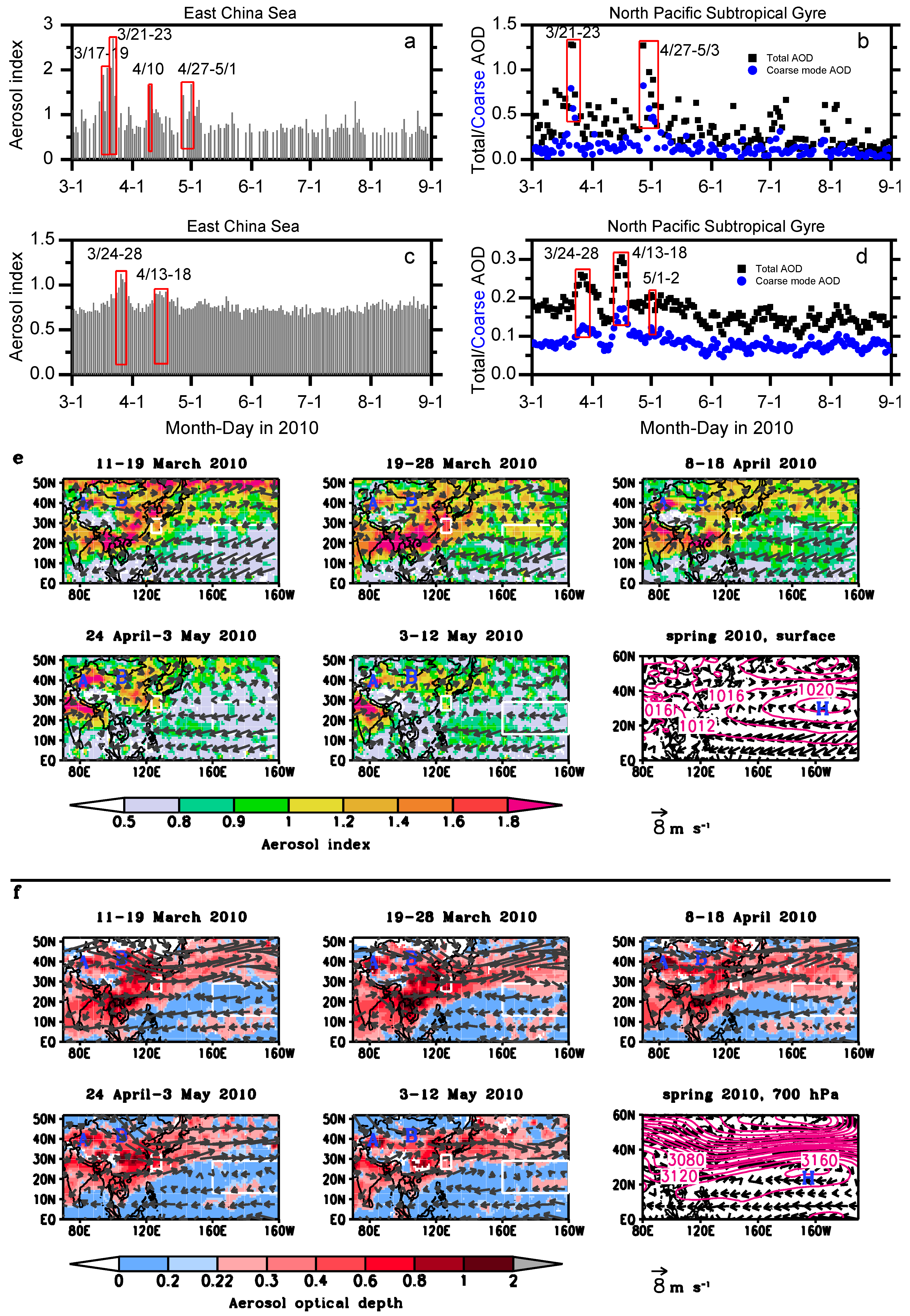
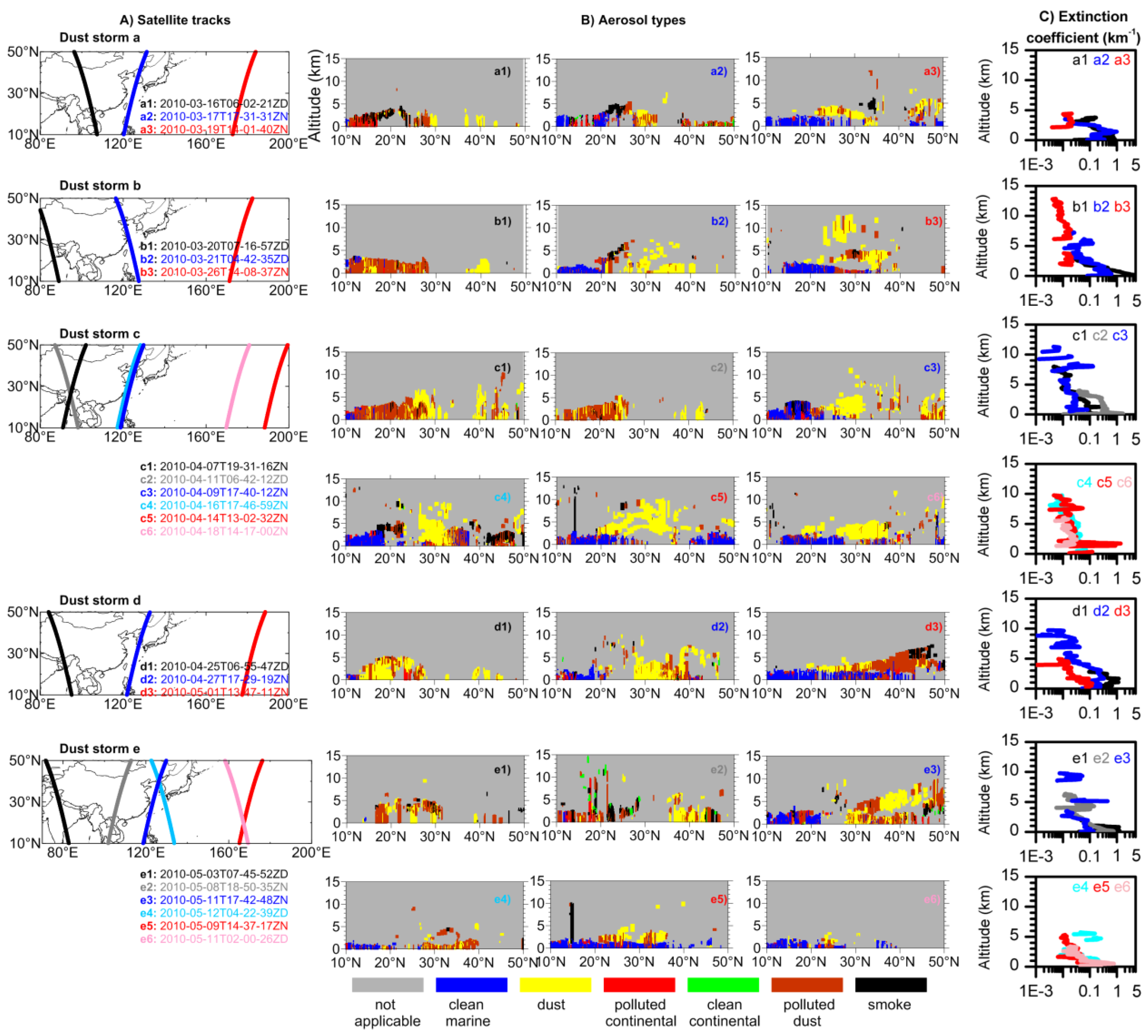
4.1. Satellite Observations of the Long-Range Transport of Dust to the ECS and the NPSG in Spring 2010

Five dust storms that passed over the ECS and the NPSG were identified by satellite instruments. The CALIOP aerosol type vertical profile data identified the date on which the dust storms passed over the seas. The spatial distribution of dust transport from the source regions to the seas were identified by the MODIS AOD and Ozone Monitoring Instrument aerosol index.
The five dust storms were labeled as dust storms (a)–(e). Based on CALIOP observations, dust storm (a) passed over the ECS from 16 to 19 March 2010 and the NPSG from 15 to 19 March 2010. The source could be the dust storm that occurred from 11 to 12 March 2010 and two blowing dust storms (see Table 2), one which occurred from 12–15 March 2010 in western and northern China and another which occurred from 16–17 March 2010 in mainly northern China [24]. This was then confirmed by the trajectories traced back to Asian dust source regions, which is described in Section 4.2 and the dust deposition flux described in Section 4.4. Dust storm (b) passed over the ECS from 20 to 23 March 2010 and the NPSG from 24 to 28 March 2010; the source could be the severe dust storm that occurred in East Asia from 19 to 22 March 2010, which has been the subject of several studies [4,5,6], and the dust storm from 21 to 23 March 2010. Dust storm (c) affected the ECS on 9–10 and 16–17 April 2010 and the NPSG on 13–18 April 2010; the source could be three blowing dust storms that occurred in western and northern China on 8, 9 and 11–12 April 2010. Dust storm (d) affected the ECS and the NPSG on some days from 26 April to 3 May 2010; the source could be the dust storm of 24–28 April 2010 recorded in the Sand Dust Weather Almanac [24]. The dust storm that occurred on 24 April 2010 in the Hexi Corridor (northern China) was called the “black storm” because the instantaneous maximum wind speed was >25 m·s−1 and the horizontal visibility was 0 m [50]. Dust storm (e) affected the ECS on 11–12 May 2010 and the NPSG on 8–11 May 2010; the source could be two blowing dust storms (3–4 and 8 May 2010) recorded in the Sand Dust Weather Almanac in 2010 [24].
Figure 2 shows the transport of the five dust storms from the source regions to the ECS and the NPSG as observed by the CALIOP instrument onboard the CALIPSO satellite. Figure 2A shows the CALIPSO satellite tracks over the source regions, the ECS, and the NPSG. The corresponding vertical cross-sections of aerosol types are shown in Figure 2B, with the bright yellow color representing the dust aerosols. The averaged profiles of the extinction coefficient at 532 nm for the dust aerosols are shown in Figure 2C. The extinction coefficient over the dust source regions (black or gray tracks in Figure 2A) was averaged between 35° and 50° N, which is the main source region for dust in East Asia. The averaged extinction coefficient over the ECS (blue tracks in Figure 2A) was calculated between 25° and 32°N and that over the NPSG (red tracks in Figure 2A) was calculated between 13° and 29°N. The altitude shown in Figure 2 is the altitude above ground level (AGL). The CALIOP data showed that dust floated from near the ground to as high as 13 km AGL in the upper free troposphere, which was consistent with previous Lidar measurements at Dunhuang, China and from Japan [51,52,53].
The averaged profiles showed that the extinction coefficient decreased with increasing altitude and decreased more rapidly in the source region. The dust storm layer at high altitude (>6 km) over the downwind sea sometimes had a similar extinction coefficient to that in the lower layer (<4 km). The mean extinction coefficient for the whole layer (0–15 km AGL) may be used to represent the mean intensity of the dust aerosol extinction coefficient and the corresponding altitude may be used to represent the mean altitude (Table 2). It is noted that a different approach was applied in case of the dispersion of volcanic aerosol layers [54]. Figure 2C shows that the dust aerosol extinction coefficient over the source region had the highest value in the layer <4 km, followed by the extinction coefficient over the ECS; the dust aerosol extinction coefficient over the NPSG had the smallest value. The mean extinction coefficient for the whole layer over the source regions varied from 0.05 to 0.96 km−1 with a mean value of 0.39 km−1 (Table 2). The maximum mean extinction coefficient was 0.96 km−1 for orbit track 2010-03-20T07-16-57ZD and next highest value was 0.53 km−1 for orbit track 2010-04-25T06-55-47ZD, which is consistent with the severe dust storm from 19 to 22 March 2010 and the dust storm from 24 to 28 April 2010. The mean extinction coefficient for the whole layer over the ECS varied from 0.02 to 0.20 km−1 with a mean value of 0.11 km−1. When dust was transported to the NPSG over a long range, the mean extinction coefficient varied from 0.01 to 0.06 km−1 with a mean of 0.02 km−1. The extinction coefficient over the source region was more than three times that over the ECS and more than one magnitude higher than that over the NPSG. The altitude at which the mean extinction coefficient was located over the source region varied from 490 to 3200 m AGL; the altitude over the ECS was around 720–4500 m AGL and that over the NPSG was around 790–6000 m AGL. On average, the altitude of the mean extinction coefficient was 1.2 km AGL over the source region, 2.3 km AGL over the ECS and 3.1 km AGL over the NPSG. These values are consistent with climatological simulations—that is, the transport of East Asian dust from the desert regions to the offshore regions near the western Pacific occurred below 3 km, whereas trans-Pacific dust transport was between 3 and 10 km [55].
The column aerosol properties, including the aerosol index and AOD (Figure 3), were also measured for the dust storms passing over the ECS and the NPSG. The daily average aerosol index and the AOD over the two sea regions showed that the aerosol index and AOD increased on the dust days and were relatively low before and after the passage of dust (Figure 3a–d). The aerosol index and AOD over the ECS on some days in the periods 17–23 March, 10 April and 27 April–2 May 2010 were >1.4 and >0.9, respectively (Figure 3a,b), although they were <1.4 and <0.9 on other days, respectively (Figure 3a,b). The NPSG, aerosol index and AOD were high on the dust passage days, particularly from 24 to 28 March and 13 to 18 April 2010 (Figure 3c,d). Dust particles are one of the most important components of the coarse aerosol mode and therefore the coarse mode AOD over the ECS and the NPSG is also shown in Figure 3b,d, respectively. Sea salt is another source of the coarse aerosol mode. The coarse mode AOD was higher during the dust days than on normal days, which further indicated that dust influenced the two sea regions on these days. Although the CALIOP instrument observed that the dust aerosol passed over the ECS and the NPSG from 8 to 12 May 2010 (Figure 2), the dust days could not be clearly distinguished from other days using the average aerosol index and the AOD, suggesting that the CALIOP instrument was able to observe more dust storm events over the downwind seas than the average aerosol index and the AOD.
The transport of dust aerosols was closely correlated with the wind speed and direction. The spatial distribution of the aerosol index and the AOD during the five dust storms indicated that dust aerosols could be transported from the source regions to the ECS by surface northwesterly winds (Figure 3e) and by westerly winds at 700 hPa (Figure 3f). When dust was transported to the North Pacific, westerly winds and an anticyclonic circulation between 20° and 40°N (Figure 3e,f) transported the dust aerosols further south below 29°N. These dust storms from 11 to 19 March and 24 April to 3 May were transported to the northern North Pacific because the westerly winds were in a more northerly location than for the dust storms from 19 to 28 March, 8 to 18 April and 3 to 12 May 2010 (Figure 3f). The stronger westerly winds at 700 hPa (Figure 3f) transported a broader dust aerosol plume across the North Pacific from 19 to 28 March and 8 to 18 April 2010 than from 3 to 12 May 2010.

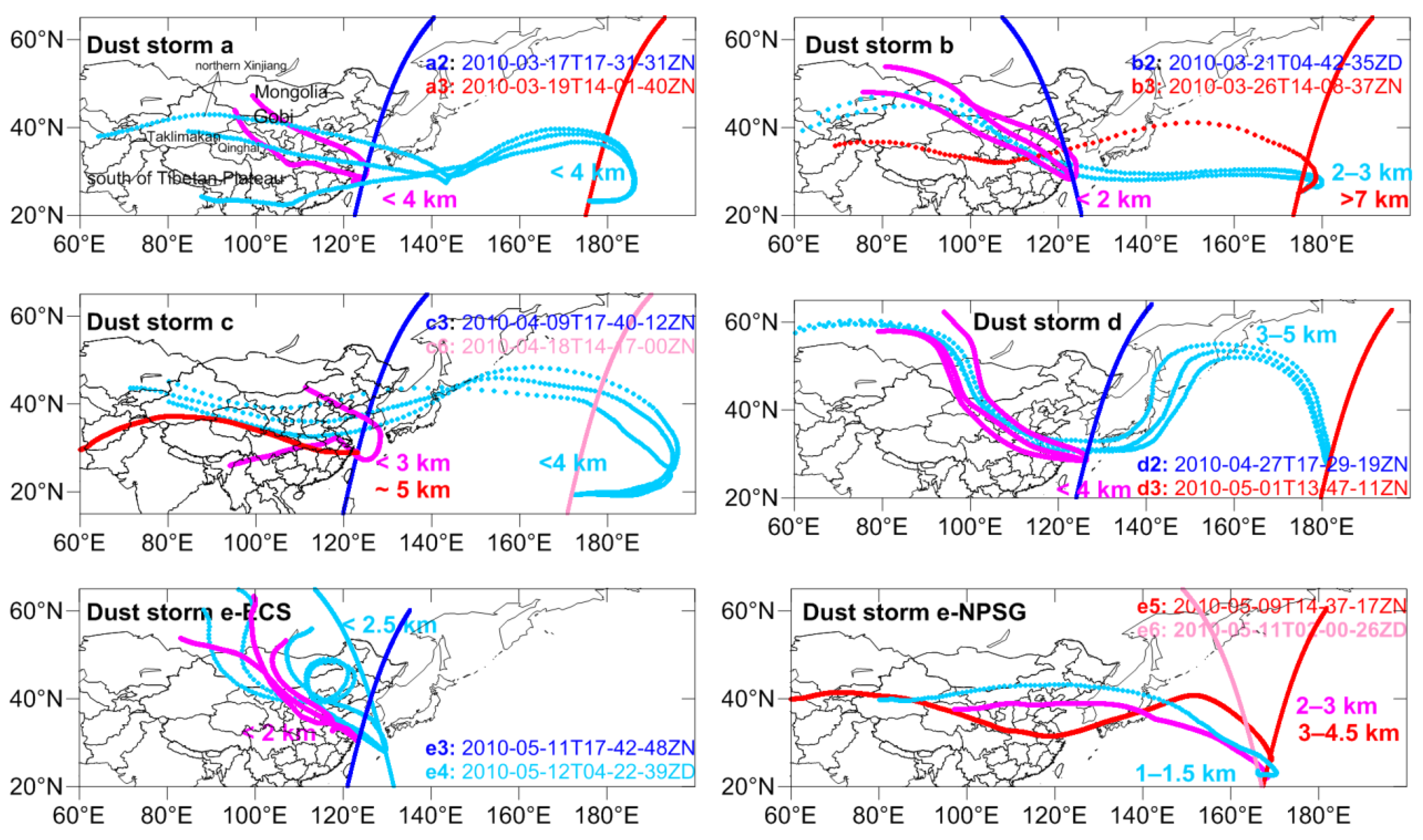
4.2. Desert Source of Dust Storms Affecting the ECS and the NPSG

Figure 4 shows the backward trajectories from the altitudes where the dust aerosols were located as observed by the CALIOP instrument (see Figure 2B). The dust aerosols for tracks a2 (2010-03-17T17-31-31ZN) and a3 (2010-03-19T17-19-25ZN) over the ECS during dust storm (a) were traced back to the Gobi Desert on 15 March 2010 and 17 March 2010, respectively. The altitude of the dust over the ECS was <4 km. For dust storm (b), the dust particles at low altitude (<3 km) over the ECS and the NPSG were traced back to the Gobi Desert on 19 March and 20 March 2010, respectively. Dust particles observed at higher altitudes (>7 km) were traced back to the Taklimakan Desert on 23 March 2010. This is consistent with previous Lidar observations and model simulations—that is, the Asian dust consisted of a multiple dust layer with the upper dust layer coming from the Taklimakan Desert and the lower dust layer from the Gobi Desert [52,53,56,57]. In a similar manner, the dust arriving at the ECS and the NPSG during dust storm events (c)–(e) could be traced back to deserts in western China (including the Taklimakan Desert and the deserts in Qinghai Province) or the Gobi region. The transport pathway to the NPSG, particularly in dust storms (a) and (c) (Figure 4), showed an anticyclonic circulation between 20° and 40° N over the North Pacific consistent with the wind directions (Figure 3e,f).
Six CALIOP profiles over the ECS (Figure 4) could be traced back to the Gobi Desert, suggesting that the Gobi Desert was the main desert source affecting the ECS. Source areas in western China and south of the Tibetan Plateau (dust storm c in Figure 4) also influenced the ECS. Five CALIOP profiles over the NPSG were traced back to deserts in western China and six CALIOP profiles were traced back to the Gobi Desert, suggesting that these two East Asian dust source regions were the main sources of dust affecting the NPSG. It was noted that this dust could mix with anthropogenic pollutants during transport before reaching the downwind sea regions [4].

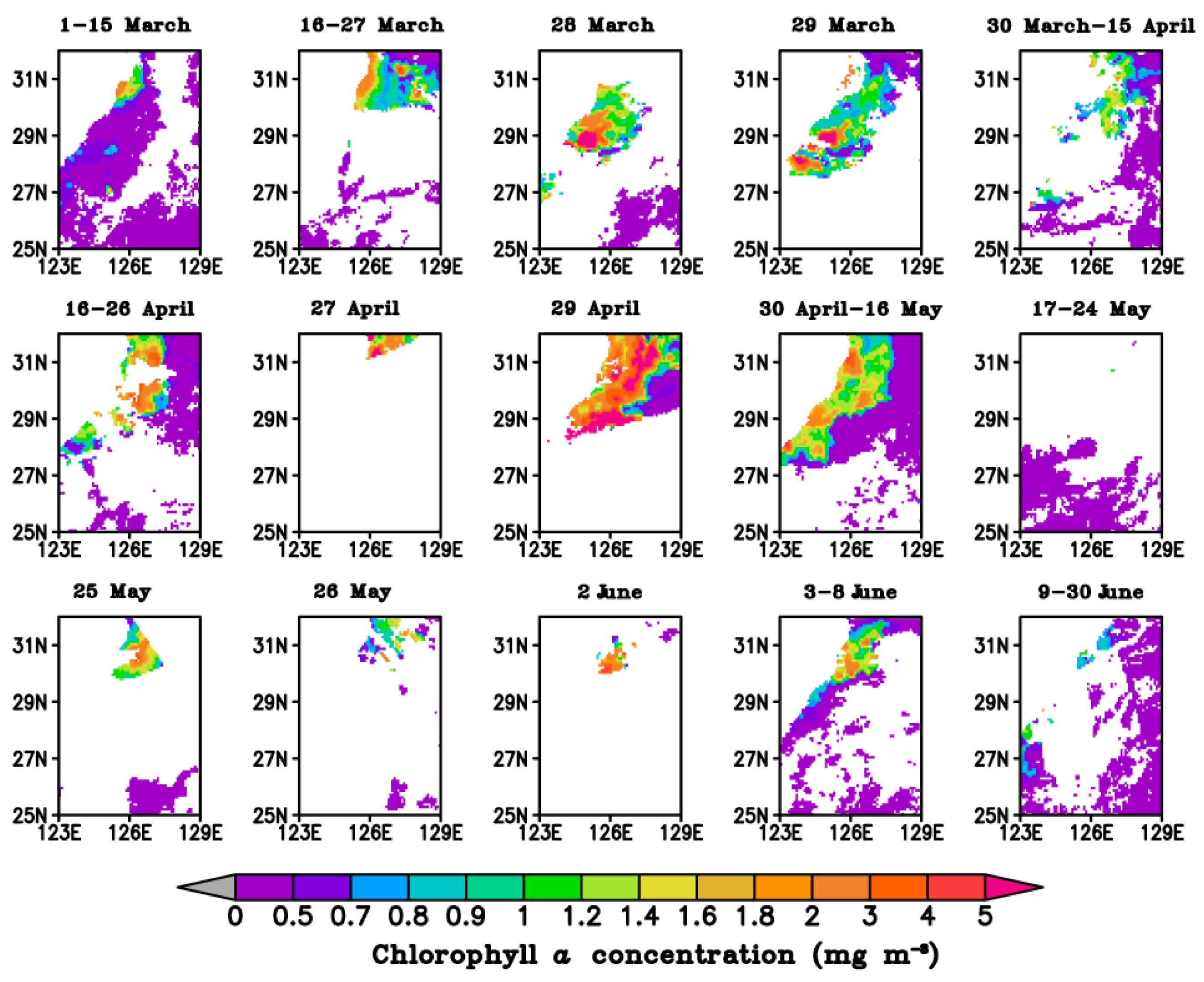
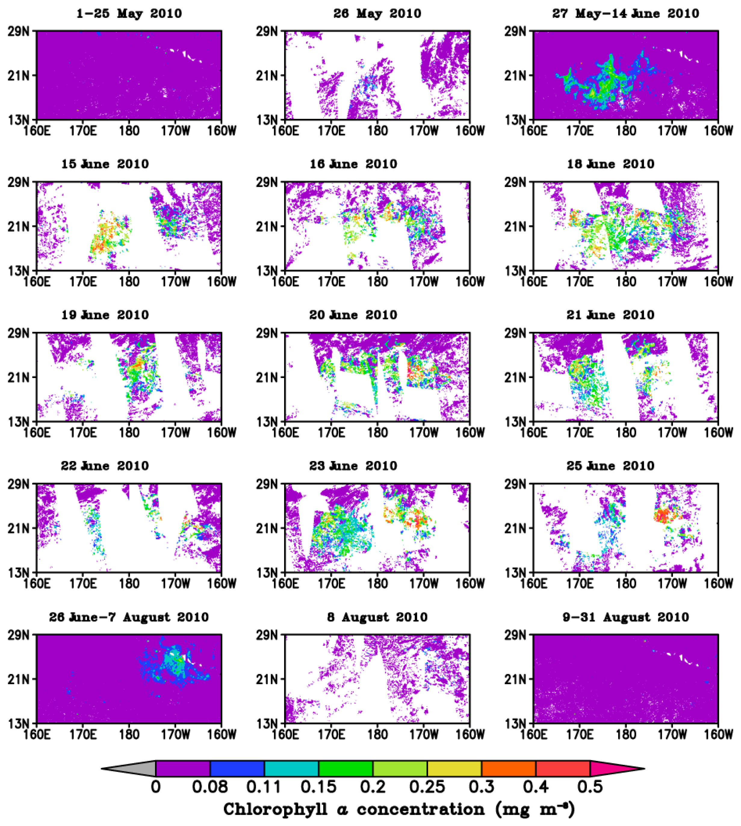
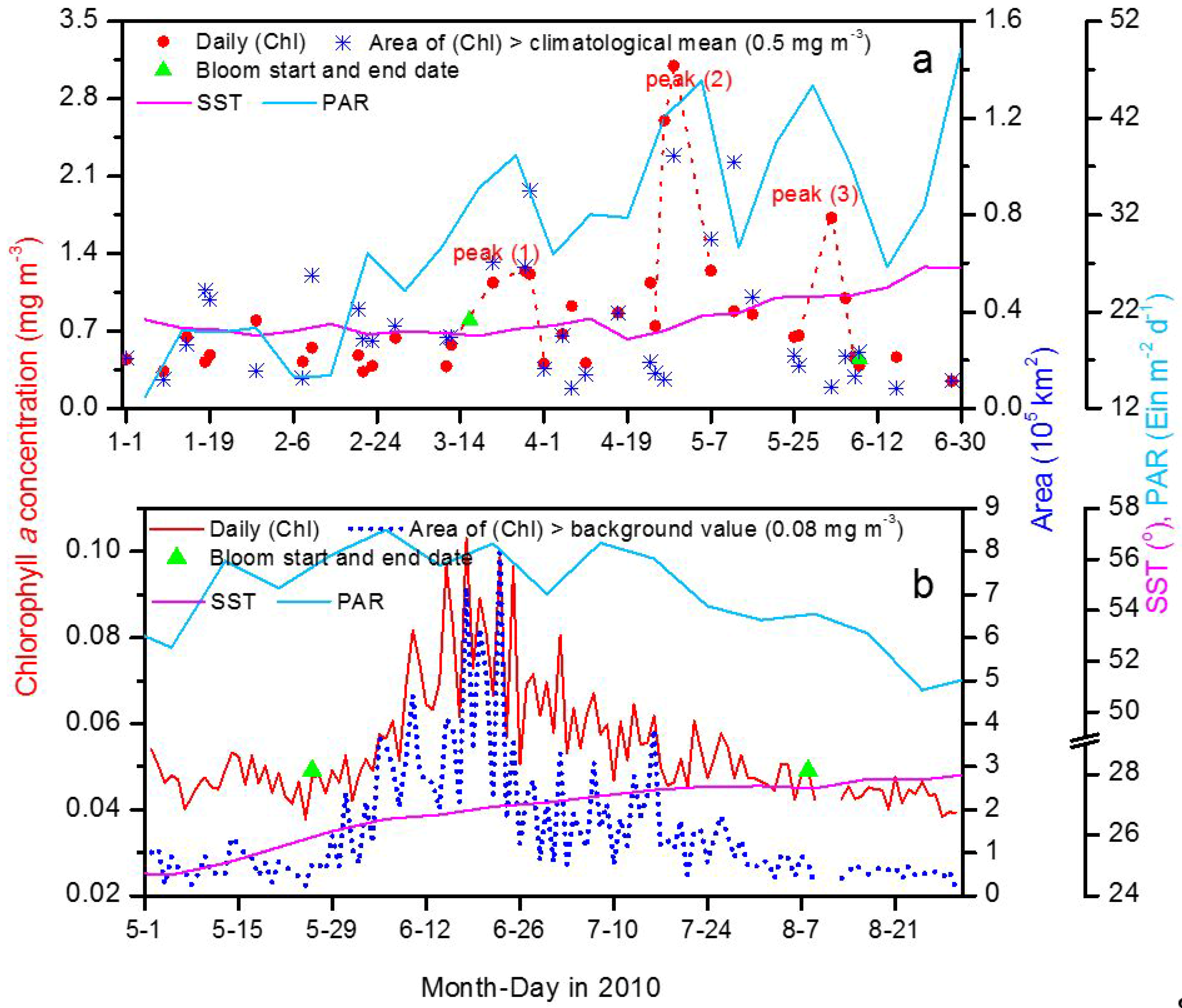
4.3. Spring Bloom in the ECS and Summer Bloom in the NPSG

The original time series of chlorophyll a concentration were analyzed to define the time of initiation of the biomass bloom. Figure 5 shows the daily mean chlorophyll a concentration and the areas in which it was higher than climatological or background level before, during and after the bloom in the ECS and the NPSG. The chlorophyll a concentration showed an initial increase in the chlorophyll a concentration to a peak, followed by a decrease over the whole period of bloom. Figure 6 and Figure 7 show daily images and the several-day average of chlorophyll a concentrations before, during and after the phytoplankton bloom in the ECS and the NPSG, respectively.
Several criteria have been used to define the timing of the initiation of the biomass bloom [12,58,59]: 5% above the yearly median of the chlorophyll a concentration (method 1) and twice the value of the wintertime chlorophyll a concentration (method 2). Different criteria may be suitable for different sea regions—for example, method 2 had been successfully used in the Sea of Japan [12] and the Yellow Sea [58]. In this study, the timing of the initiation and end of the spring bloom in the ECS was defined by method 2 (see Figure 5a and Figure 6). The timing of the initiation of the spring bloom defined by methods 2 (0.8 mg·m−3) was on 16 March; it seems suitable since the day was within non-bloom day (12 March) and high concentration day (21 March) (Figure 5a). When method 1 (0.4 mg·m−3) was used in the ECS, the values were too low and every day of spring 2010 was identified as a bloom event. In the NPSG, method 1 (0.049 mg·m−3) was suitable for defining the initiation of the summer 2010 bloom (see Figure 5b and Figure 7). The timing of the end of the bloom was defined as the day on which the chlorophyll a concentration decreased to the same value as on the initiation date. The concentration defined by method 2 (0.12 mg·m−3) was too high and no bloom was detected. Once the initiation and end of the bloom had been determined, the duration of the spring bloom in the ECS and the summer bloom in the NPSG were identified (Figure 5).
The 2010 spring bloom in the ECS started on about 16 March and ended on about 8 June and chlorophyll a concentration had three peaks during this period (Figure 5a). The phytoplankton grew to a peak and then declined; this growth process was then repeated twice more. During the three growth processes, the original chlorophyll a concentration time series showed high values on 28 March (1.24 mg·m−3), 29 April (3.10 mg·m−3) and 2 June (1.72 mg·m−3). The first peak was comparable with the third peak and the second peak was the highest. The daily images clearly show the three growth and decay periods (Figure 6). The chlorophyll a concentration before the first growth period was lower than the springtime climatological mean of 0.5 mg·m−3 except in the northwestern region. The chlorophyll a concentration increased gradually and reached the highest value in the center of the research region on 28 and 29 March 2010, before decaying from 30 March to 15 April 2010. The chlorophyll a concentration then began to increase again from 16 to 26 April and reached the highest values in the center and north of the research region on 29 April before decreasing again from 30 April to 24 May 2010. The satellite data for the chlorophyll a concentration in the bloom region from 17 to 24 May 2010 were almost absent; only several pixels were >1 mg·m−3 in the bloom region, thus bloom should still exist during 17–24 May. The third growth process began on 25 May 2010, peaked on 2 June 2010, and then decayed from 3 to 8 June 2010. After the spring bloom, the chlorophyll a concentration decreased to <0.5 mg·m−3.
The chlorophyll a concentration in the NPSG increased to a peak followed by a decrease in summer 2010 (Figure 5b). The bloom started from 26 May 2010 based on the 5% criterion and the chlorophyll a concentration was 0.048 mg·m−3 on that day. The initiation date was similar to that derived from the eight-day chlorophyll a concentration, i.e., 17 May (actually the 8-day from 17 to 24 May) [15]. The phytoplankton growth reached a peak one month later. The period with high chlorophyll a concentrations lasted from 15 to 25 June 2010. The four highest chlorophyll a concentrations appeared on 18 June (0.103 mg·m−3), 23 June (0.099 mg·m−3), 15 June (0.097 mg·m−3) and 25 June (0.097 mg·m−3). After the peak, the chlorophyll a concentration decreased day by day and the bloom began to fade on 8 August 2010 (0.049 mg·m−3). The bloom area, represented by the area with chlorophyll a concentrations higher than the background value of 0.08 mg·m−3, increased from 0.75 × 10⁵ km2 on 26 May to a peak of 8.08 × 10⁵ km2 on 23 June and then decreased to 0.74 × 10⁵ km2 on 8 August 2010. The peak area was consistent with the 8 × 10⁵ km2 area reported by Calil et al. [15].
The spatial distribution of the chlorophyll a concentration (Figure 7) showed that the average chlorophyll a concentration was lower than the background value both before and after the bloom. During the period of high chlorophyll a concentration, the concentration was >0.4 mg·m−3, a high value for oligotrophic oceans. The bloom started from the southwest of the research region (around 175°–180°E, 16°–21°N) and spread over almost the whole region before fading in the northeast of the region (Figure 7). Calil et al. [15] suggested that a possible reason for the eastward displacement of the bloom was seasonal buoyancy forcing and transport by the Hawaiian Lee Counter Current, although the second hypothesis was argued against by float experiments. The 2010 bloom lasted about 75 days, which is reasonable compared with the duration of the bloom east of 160° W, which commonly lasts four to six weeks and sometimes up to four months [47,48].
The chlorophyll a concentration increased with increases in the SST and the PAR (Figure 5), suggesting that particular SSTs and light levels are required by phytoplankton. Phytoplankton also require basic nutrients such as nitrogen, phosphorus and iron. The nutrients may be delivered from subsurface waters via upwelling [15] or by atmospheric deposition.

4.4. Simulated Dust Deposition, Estimations of Nutrients and Their Contribution to Biological Productivity

Figure 8 shows an example of the total dust deposition in the ECS and the NPSG simulated by the RAQMS model for one dust storm event together with the maximum flux. Based on the RAQMS model, the dust deposition flux in the ECS for the five dust storms ranged from 13.0 to 145.6 mg·m−2·d−1. The mean amount of deposition and the deposition flux for the five dust storms were about 284.3 mg·m−2 and 64.7 mg·m−2·d−1 (40.0 and 24.7 mg·m−2·d−1 for dry and wet deposition, respectively). The dry deposition flux was slightly lower than the mean value of 50 mg·m−2·d−1 derived from the aerosol samples between 21 and 29 March 2010 in northern Taiwan [60]. The mean dry deposition, including both severe and weak dust storm events, appears to be reasonable because the dust storm from 21 to 29 March 2010 was a severe event. The simulated total dust deposition in the NPSG for five dust storms varied from 2.2 to 33.1 mg·m−2 with a mean value of 14.8 mg·m−2 and the corresponding flux was about 0.6–5.5 mg·m−2·d−1 with a mean value of 2.8 mg·m−2·d−1. This was of the same magnitude as the mean deposition (20 mg·m−2) simulated by the SPRINTAS model over a similar region (160°E to 160°W, 15°–30°N) for two dust events from 14 to 16 April and 1 to 4 May 2010 [15].
The deposition of dust during the bloom period supplied nutrients in the form of iron, nitrogen and phosphorus to support phytoplankton growth. The impact of these dust events on the biomass of phytoplankton was estimated by quantifying the solubility of the iron and phosphorus derived from the dust and assuming that all the soluble iron and phosphorus was bioavailable; this is the most common approach to examining the delivery of aerosol iron to phytoplankton [23]. A series of conversion ratios from previous studies was used to estimate the effects of dust on the biomass of phytoplankton. The average iron content of soil dust (3.5% by weight) [10] and the phosphorus (0.053%) and total inorganic nitrogen (1%) content of dust particles measured from a dust event in spring 2007 over the Yellow Sea [19] were used. The solubility of iron is highly variable and the value used in biogeochemical modeling studies has varied from 1% to 12% [23]. The solubility of iron derived from ship-based measurements in the marginal seas of China ranged from 1% to 2.6%, with a mean value of 1.65% for dust particles in spring 2007 over the Yellow Sea [19]. Some studies have reported that the solubility of iron in the remote ocean is higher than that in Mainland China [61] and this has been confirmed by model simulations [4]. The 5% solubility value reported by Li et al. [4] close to the west of the NPSG was used for the NPSG. The solubility of phosphorus (30%) has been estimated from dust aerosol samples [62] and was comparable with the value of 32% measured in marine aerosols over the Atlantic Ocean [63]. The median value of the measured iron to carbon ratio of 38 μmol Fe:mol C [64], a carbon to chlorophyll (Chl) ratio of 50 g C:g Chl [65] and a Redfield ratio of C:N:P of 106:16:1 were used. The median value (22 m) of the mixed layer depth of the ocean measured in the ECS in spring [66] and a typical summertime mixed layer depth (40 m) at Station ALOHA in the NPSG [15] were used and the biomass was assumed to be spread homogeneously within the mixed layer.
Using these parameters, the estimated amount of soluble iron supported by the mean dust deposition flux (64.7 mg·m−2·d−1) over the ECS was calculated to be 37.5 μg·m−2·d−1 (Table 3), which was comparable with the mean value of 39 μg·m−2·d−1 obtained by Hsu et al. [62] in the northeasterly monsoon periods. Soluble phosphorus (10.3 μg·m−2·d−1) was more than three times higher than the mean value of 3.3 μg·m−2·d−1 derived by Hsu et al. [62] from dry deposition in the northeasterly monsoon period. The amount of soluble phosphorus of 10.3 μg·m−2·d−1 corresponds to 0.95 mg·m−2 in spring 2010, which accounts for 63% of the yearly dry deposition of dissolved inorganic phosphorus from dust storm samples (1.5 mg·m−2) obtained by Chen and Chen [67]. The total estimated deposition of total inorganic nitrogen supported by a mean dust deposition flux of 64.7 mg·m−2·d−1was 0.6 mg·m−2·d−1, which was comparable with the mean value of 0.69 mg·m−2·d−1 previously derived from dry deposition over the ECS [62]. These comparisons show that our simulations are reasonable.
The amounts of bioavailable nutrients supplied by the weakest and most severe dust storm events were then calculated (Table 3) and their role in supporting the 2010 bloom in the two sea regions considered. The mean increase in the chlorophyll a concentration over the ECS for three growth periods in spring 2010 was about 1.5 mg·m−3 and the estimated amount of new production in spring was 209 mg C m−2·d−1[66]. The amount of new production supported by iron deposition from the five dust storm events in the ECS varied from 42.34 to 474.16 mg C m−2·d−1 (mean 210.70 mg C m−2·d−1), which represents 20%–227% (mean 101%) of the new springtime production. Iron deposition in the ECS could produce 0.08–1.72 mg·m−3 of chlorophyll a (mean 0.84), accounting for 5%–115% (mean 56%) of the mean increase in chlorophyll a concentration in spring 2010. The total inorganic nitrogen deposition from five dust storm events may have supported 0.74–8.27 mg C m−2·d−1 of new production (0.4%–4.0% of the new springtime production). The contribution ratio of new production produced by total inorganic nitrogen deposition from one dust storm event is reasonable compared with the 1.1%–3.9% from the simulated atmospheric deposition of the total annual nitrogen [45]. The deposition of soluble phosphorus can support 0.08–0.95 mg C m−2·d−1 of new production, accounting for 0.04%–0.5% of the new springtime production. The contribution ratio of total inorganic nitrogen and soluble phosphorus supported by the five dust storms to the mean increase in chlorophyll a concentration varied from 0.1% to 2.0% and 0.01% to 0.2%, respectively, which is similar to the contribution ratio for the new springtime production. As a result, the atmospheric deposition of iron is seen to be the most important factor in phytoplankton growth in the ECS; nitrogen also plays an important part, whereas phosphorus has less impact. Previous studies have indicated that atmospheric phosphorus may not be a vital source of inorganic phosphorus in the ECS [62,67].
During the 2010 summer phytoplankton bloom in the NPSG, the maximum chlorophyll a concentration increased by 0.056 mg·m−3 relative to that before bloom. The soluble iron, soluble phosphorus and total inorganic nitrogen from dust deposition into the NPSG of 2.2–33.1 mg·m−2 (mean 14.8 mg·m−2) may have contributed 19%–291% (mean 130%), 0.01%–0.2% (mean 0.1%) and 0.1%–1.7% (mean 0.8%), respectively, of the increase in the chlorophyll a concentration in summer 2010 (Table 3). This suggests that the bloom in the NPSG could be largely supported by the iron deposited from one dust storm episode, followed by nitrogen and then phosphorus deposition. Calil et al. [15] showed that phosphate could have been supplied by episodic upwelling induced by frontogenetically generated vertical velocities.

5. Conclusions

The transport, deposition and impacts of five dust storm events on the ECS (a marginal sea) and the NPSG (a typical low nutrient–low chlorophyll open ocean) were compared using a variety of data, including the column AOD and aerosol index measured by satellite, the vertical distribution of aerosol types and the extinction coefficient measured by satellite, satellite ocean color data, simulated dust deposition and backward trajectories. Several similarities and differences were observed between the two seas.
The source region, extinction coefficient and transport altitude of dust aerosols were different between the two seas. Based on a limited number of cases, the East Asian dust affecting the ECS mainly came from the Gobi Desert and secondly came from deserts in western China. The deserts in western China and the Gobi region were the main sources of dust affecting the NPSG. The mean extinction coefficient of the dust aerosol for the whole layer over the ECS (0.11 km−1) is about one order of magnitude higher than over the NPSG (0.02 km−1). The transport of East Asian dust from the desert regions to the ECS occurred below 4 km, whereas transport to the NPSG occurred at higher altitudes.
The growth of phytoplankton was different in the two seas. The phytoplankton bloom in the ECS and the west of the NPSG lasted for more than two months. During the bloom period, the phytoplankton in the ECS experienced three growth periods in which the blooms grew to a peak and then decreased. The chlorophyll a concentration during the bloom period in the NPSG showed an initial increase to a peak, followed by a decrease. Dust frequently intruded during the bloom period in the ECS and may have continuously provided nutrients for the phytoplankton bloom. After dust deposition in the spring, the bloom in the NPSG did not start until the SST and light levels reached an optimum value.
The contributions of the deposition of nutrients (nitrogen, phosphorus and iron) to phytoplankton growth in the two seas were similar. The simulated total dust deposition flux was up to 145.6 mg·m−2·d−1 in the ECS and up to 5.5 mg·m−2·d−1 in the NPSG. Our results suggested that the atmospheric deposition of iron was the most important factor in phytoplankton growth in the ECS and accounted for up to 227% of the new springtime production and up to 115% of the mean increase in chlorophyll a concentration in spring 2010. The new production produced by the atmospheric deposition of total inorganic nitrogen and soluble phosphorus accounted for up to 4.0% and 0.5% of the new springtime production in the ECS, respectively. The deposition of soluble iron, soluble phosphorus and total inorganic nitrogen into the NPSG could have produced up to 291, 0.2% and 1.7%, respectively, of the increase in the chlorophyll a concentration in summer 2010, suggesting that dust containing iron was also the most important factor affecting phytoplankton growth in the NPSG and that nitrogen was the second most important factor.
This study showed that the active remote sensing is very important as it can identify dust aerosol vertically. In the future, the spaceborne Lidars [68] and ground-based networks of Lidars/ceilometers [69] may improve our understanding of the impact of dust deposition on marine biological activity. They can be used to better monitor the origin of dust layers and their transport paths; and can be used to validate models (e.g., Müller et al. [70] and Emeis et al. [71]).

Acknowledgments

This work was supported by the Ministry of Science and Technology of China (grant No. 2014CB953703), the National Natural Science Foundation of China (grant No. 41590874 and 41210008), the National Key R & D Program Pilot Projects of China (grant No. 2016YFA060191), and the Open Research Program of the State Key Laboratory of Satellite Ocean Environment Dynamics, Second Institute of Oceanography, State Oceanic Administration (grant No. SOED1504). We also thank the Ocean Biology Processing Group of NASA’s GSFC for the ocean color data, the Ozone Processing Team of NASA GSFC for the aerosol index data and the Level 1 and Atmosphere Archive and Distribution System web of NASA GSFC for the AOD data. The authors gratefully acknowledge the NOAA Air Resources Laboratory for the provision of the HYSPLIT transport and dispersion model used in this research. Thank Ms. Ammara Habib for formatting this manuscript.

Author Contributions

Saichun Tan and Huiwang Gao conceived and designed the research; Jiawei Li run the Regional Air Quality Model System numerical model; Hong Wang contributed analysis tools; Huizheng Che and Bin Chen analyzed the data; and Saichun Tan performed the experiments and wrote the paper.

Conflicts of Interest

The authors declares no conflict of interest.

References

  1. Zhang, X.Y.; Gong, S.-L.; Zhao, T.-L.; Arimoto, R. Sources of asian dust and role of climate change versus desertification in Asian dust emission. Geophys. Res. Lett. 2003, 30, 2272. [Google Scholar] [CrossRef]
  2. China Meteorological Administration (CMA). Grade of Sand and Dust Storm Weather, National Standard of the People’s Republic of China; gb/t 20480-2006; China Meteorological Administration (CMA), Standardization Administration of China (SAC): Beijing, China, 2006. (In Chinese)
  3. Li, J.; Han, Z.; Zhang, R. Model study of atmospheric particulates during dust storm period in March 2010 over east asia. Atmos. Environ. 2011, 45, 3954–3964. [Google Scholar] [CrossRef]
  4. Li, J.; Wang, Z.; Zhuang, G.; Luo, G.; Sun, Y.; Wang, Q. Mixing of asian mineral dust with anthropogenic pollutants over east Asia: A model case study of a super-duststorm in March 2010. Atmos. Chem. Phys. 2012, 12, 7591–7607. [Google Scholar] [CrossRef]
  5. Wang, S.-H.; Hsu, N.C.; Tsay, S.-C.; Lin, N.-H.; Sayer, A.M.; Huang, S.-J.; Lau, W.K.M. Can asian dust trigger phytoplankton blooms in the oligotrophic northern South China Sea? Geophys. Res. Lett. 2012, 39, L05811. [Google Scholar] [CrossRef]
  6. Tan, S.-C.; Wang, H. The transport and deposition of dust and its impact on phytoplankton growth in the Yellow Sea. Atmos. Environ. 2014, 99, 491–499. [Google Scholar] [CrossRef]
  7. Martin, J.H.; Fitzwater, S.E. Iron deficiency limits phytoplankton growth in the North-East Pacific Subarctic. Nature 1988, 331, 341–343. [Google Scholar] [CrossRef]
  8. Behrenfeld, M.J.; Bale, A.J.; Kolber, Z.S.; Aiken, J.; Falkowski, P.G. Confirmation of iron limitation of phytoplankton photosynthesis in the equatorial Pacific Ocean. Nature 1996, 383, 508–511. [Google Scholar] [CrossRef]
  9. Boyd, P.W. Ironing out algal issues in the Southern Ocean. Science 2004, 304, 396–397. [Google Scholar] [CrossRef] [PubMed]
  10. Jickells, T.D.; An, Z.S.; Andersen, K.K.; Baker, A.R.; Bergametti, G.; Brooks, N.; Cao, J.J.; Boyd, P.W.; Duce, R.A.; Hunter, K.A.; et al. Global iron connections between desert dust, ocean biogeochemistry, and climate. Science 2005, 308, 67–71. [Google Scholar] [CrossRef] [PubMed]
  11. Yuan, W.; Zhang, J. High correlations between asian dust events and biological productivity in the Western North Pacific. Geophys. Res. Lett. 2006, 33, L07603. [Google Scholar] [CrossRef]
  12. Jo, C.-O.; Lee, J.-Y.; Park, K.-A.; Kim, Y.-H.; Kim, K.-R. Asian dust initiated early spring bloom in the Northern East/Japan Sea. Geophys. Res. Lett. 2007, 34, L05602. [Google Scholar] [CrossRef]
  13. Duce, R.A.; LaRoche, J.; Altieri, K.; Arrigo, K.R.; Baker, A.R.; Capone, D.G.; Cornell, S.; Dentener, F.; Galloway, J.; Ganeshram, R.S.; et al. Impacts of atmospheric anthropogenic nitrogen on the open ocean. Science 2008, 320, 893–897. [Google Scholar] [CrossRef] [PubMed]
  14. Gabric, A.J.; Cropp, R.A.; McTainsh, G.H.; Johnston, B.M.; Butler, H.; Tilbrook, B.; Keywood, M. Australian dust storms in 2002–2003 and their impact on Southern Ocean biogeochemistry. Glob. Biogeochem. Cycles 2010, 24, GB2005. [Google Scholar] [CrossRef]
  15. Calil, P.H.R.; Doney, S.C.; Yumimoto, K.; Eguchi, K.; Takemura, T. Episodic upwelling and dust deposition as bloom triggers in low-nutrient, low-chlorophyll regions. J. Geophys. Res. 2011, 116, C06030. [Google Scholar] [CrossRef]
  16. Shi, J.-H.; Gao, H.-W.; Zhang, J.; Tan, S.-C.; Ren, J.-L.; Liu, C.-G.; Liu, Y.; Yao, X. Examination of causative link between a spring bloom and dry/wet deposition of Asian dust in the Yellow Sea, China. J. Geophys. Res. 2012, 117, D17304. [Google Scholar] [CrossRef]
  17. Furutani, H.; Meguro, A.; Iguchi, H.; Uematsu, M. Geographical distribution and sources of phosphorus in atmospheric aerosol over the North Pacific Ocean. Geophys. Res. Lett. 2010, 37, L03805. [Google Scholar] [CrossRef]
  18. Kim, T.-W.; Lee, K.; Najjar, R.G.; Jeong, H.-D.; Jeong, H.J. Increasing N abundance in the Northwestern Pacific Ocean due to atmospheric nitrogen deposition. Science 2011, 334, 505–509. [Google Scholar] [CrossRef] [PubMed]
  19. Shi, J.-H.; Zhang, J.; Gao, H.-W.; Tan, S.-C.; Yao, X.-H.; Ren, J.-L. Concentration, solubility and deposition flux of atmospheric particulate nutrients over the Yellow Sea. Deep Sea Res. Part II Top. Stud. Oceanogr. 2013, 97, 43–50. [Google Scholar] [CrossRef]
  20. Bishop, J.K.B.; Davis, R.E.; Sherman, J.T. Robotic observations of dust storm enhancement of carbon biomass in the North Pacific. Science 2002, 298, 817–821. [Google Scholar] [CrossRef] [PubMed]
  21. Han, Y.; Zhao, T.; Song, L.; Fang, X.; Yin, Y.; Deng, Z.; Wang, S.; Fan, S. A linkage between Asian dust, dissolved iron and marine export production in the deep ocean. Atmos. Environ. 2011, 45, 4291–4298. [Google Scholar] [CrossRef]
  22. Tan, S.-C.; Yao, X.; Gao, H.-W.; Shi, G.-Y.; Yue, X. Variability in the correlation between Asian dust storms and chlorophyll a concentration from the north to equatorial Pacific. PLoS ONE 2013, 8, e57656. [Google Scholar] [CrossRef] [PubMed]
  23. Boyd, P.W.; Mackie, D.S.; Hunter, K.A. Aerosol iron deposition to the surface ocean—Modes of iron supply and biological responses. Mar. Chem. 2010, 120, 128–143. [Google Scholar] [CrossRef]
  24. China Meteorological Administration (CMA). Sand Dust Weather Almanac; China Meteorological Administration (CMA), China Meteorological Press: Beijing, China, 2010. (In Chinese)
  25. Lin, C.Y.; Sheng, Y.F.; Chen, W.N.; Wang, Z.; Kuo, C.H.; Chen, W.C.; Yang, T. The impact of channel effect on Asian dust transport dynamics: A case in Southeastern Asia. Atmos. Chem. Phys. 2012, 12, 271–285. [Google Scholar] [CrossRef]
  26. Winker, D.M.; Vaughan, M.A.; Omar, A.; Hu, Y.; Powell, K.A.; Liu, Z.; Hunt, W.H.; Young, S.A. Overview of the calipso mission and caliop data processing algorithms. J. Atmos. Ocean. Technol. 2009, 26, 2310–2323. [Google Scholar] [CrossRef]
  27. Amiridis, V.; Wandinger, U.; Marinou, E.; Giannakaki, E.; Tsekeri, A.; Basart, S.; Kazadzis, S.; Gkikas, A.; Taylor, M.; Baldasano, J.; et al. Optimizing Calipso Saharan dust retrievals. Atmos. Chem. Phys. 2013, 13, 12089–12106. [Google Scholar] [CrossRef] [Green Version]
  28. Papagiannopoulos, N.; Mona, L.; Alados-Arboledas, L.; Amiridis, V.; Baars, H.; Binietoglou, I.; Bortoli, D.; D’Amico, G.; Giunta, A.; Guerrero-Rascado, J.L.; et al. Calipso climatological products: Evaluation and suggestions from earlinet. Atmos. Chem. Phys. 2016, 16, 2341–2357. [Google Scholar] [CrossRef]
  29. Murayama, T.; Müller, D.; Wada, K.; Shimizu, A.; Sekiguchi, M.; Tsukamoto, T. Characterization of Asian dust and siberian smoke with multi-wavelength raman Lidar over Tokyo, Japan in spring 2003. Geophys. Res. Lett. 2004, 31, L23103. [Google Scholar] [CrossRef]
  30. Liu, Z.; Sugimoto, N.; Murayama, T. Extinction-to-backscatter ratio of asian dust observed with high-spectral-resolution Lidar and raman Lidar. Appl. Opt. 2002, 41, 2760–2767. [Google Scholar] [CrossRef] [PubMed]
  31. Uno, I.; Yumimoto, K.; Shimizu, A.; Hara, Y.; Sugimoto, N.; Wang, Z.; Liu, Z.; Winker, D.M. 3D structure of Asian dust transport revealed by CALIPSO Lidar and a 4DVAR dust model. Geophys. Res. Lett. 2008, 35, L06803. [Google Scholar] [CrossRef]
  32. Torres, O.; Tanskanen, A.; Veihelmann, B.; Ahn, C.; Braak, R.; Bhartia, P.K.; Veefkind, P.; Levelt, P. Aerosols and surface UV products from ozone monitoring instrument observations: An overview. J. Geophys. Res. 2007, 112, D24S47. [Google Scholar] [CrossRef]
  33. Prospero, J.M.; Ginoux, P.; Torres, O.; Nicholson, S.E.; Gill, T.E. Environmental characterization of global sources of atmospheric soil dust identified with the NIMBUS-7 total ozone mapping spectrometer (TOMS) absorbing aerosol product. Rev. Geophys. 2002, 40, 1002. [Google Scholar] [CrossRef]
  34. Draxler, R.R.; Rolph, G.D. Hysplit (Hybrid Single-Particle Lagrangian Integrated Trajectory) Model Access via NOAA Arl Ready Website; NOAA Air Resources Laboratory: Silver Spring, MD, USA, 2010.
  35. Grell, G.A.; Dudhia, J.; Stauffer, D.R. A Description of the Fifth-Generation Penn State/NCAR Mesoscale Model (MM5); NCAR Technical Note, NCAR/TN-398+STR; The National Center for Atmospheric Research (NCAR): Boulder, CO, USA, 1994. [Google Scholar]
  36. Han, Z. A regional air quality model: Evaluation and simulation of O3 and relevant gaseous species in East Asia during spring 2001. Environ. Model. Softw. 2007, 22, 1328–1336. [Google Scholar] [CrossRef]
  37. Han, Z.; Xie, Z.; Wang, G.; Zhang, R.; Tao, J. Modeling organic aerosols over east china using a volatility basis-set approach with aging mechanism in a regional air quality model. Atmos. Environ. 2016, 124 Pt B, 186–198. [Google Scholar] [CrossRef]
  38. Huang, M.; Wang, Z.; He, D.; Xu, H.; Zhou, L. Modeling studies on sulfur deposition and transport in East Asia. Water Air Soil Pollut. 1995, 85, 1921–1926. [Google Scholar]
  39. Gong, G.-C.; Wen, Y.-H.; Wang, B.-W.; Liu, G.-J. Seasonal variation of chlorophyll a concentration, primary production and environmental conditions in the subtropical East China Sea. Deep Sea Res. Part II Top. Stud. Oceanogr. 2003, 50, 1219–1236. [Google Scholar] [CrossRef]
  40. Ning, X.; Liu, Z.; Cai, Y.; Fang, M.; Chai, F. Physicobiological oceanographic remote sensing of the East China Sea: Satellite and in situ observations. J. Geophys. Res. 1998, 103, 21623–21635. [Google Scholar] [CrossRef]
  41. Li, G.-X.; Han, X.-B.; Yue, S.-H.; Wen, G.-Y.; Yang, R.-M.; Kusky, T.M. Monthly variations of water masses in the East China Seas. Cont. Shelf Res. 2006, 26, 1954–1970. [Google Scholar] [CrossRef]
  42. Singh, R.P.; Prasad, A.K.; Kayetha, V.K.; Kafatos, M. Enhancement of oceanic parameters associated with dust storms using satellite data. J. Geophys. Res. 2008, 113, C11008. [Google Scholar] [CrossRef]
  43. Wang, B.-D.; Wang, X.-L.; Zhan, R. Nutrient conditions in the yellow sea and the east china sea. Estuar. Coast. Shelf Sci. 2003, 58, 127–136. [Google Scholar] [CrossRef]
  44. Chen, C.-T.A. Distributions of nutrients in the East China Sea and the South China Sea connection. J. Oceanogr. 2008, 64, 737–751. [Google Scholar] [CrossRef]
  45. Zhang, Y.; Yu, Q.; Ma, W.; Chen, L. Atmospheric deposition of inorganic nitrogen to the Eastern China Seas and its implications to marine biogeochemistry. J. Geophys. Res. 2010, 115, D00K10. [Google Scholar] [CrossRef]
  46. Karl, D.M.; Letelier, R.M. Nitrogen fixation-enhanced carbon sequestration in low nitrate, low chlorophyll seascapes. Mar. Ecol. Prog. Ser. 2008, 364, 257–268. [Google Scholar] [CrossRef]
  47. Wilson, C. Late summer chlorophyll blooms in the oligotrophic North Pacific Subtropical Gyre. Geophys. Res. Lett. 2003, 30, 1942. [Google Scholar] [CrossRef]
  48. Wilson, C.; Villareal, T.A.; Maximenko, N.; Bograd, S.J.; Montoya, J.P.; Schoenbaechler, C.A. Biological and physical forcings of late summer chlorophyll blooms at 30° N in the oligotrophic Pacific. J. Mar. Syst. 2008, 69, 164–176. [Google Scholar] [CrossRef]
  49. Dore, J.E.; Letelier, R.M.; Church, M.J.; Lukas, R.; Karl, D.M. Summer phytoplankton blooms in the oligotrophic North Pacific Subtropical Gyre: Historical perspective and recent observations. Prog. Oceanogr. 2008, 76, 2–38. [Google Scholar] [CrossRef]
  50. Qian, L.; Yang, Y.-L.; Wang, R.-Z. Analysis on black storm cause in Hexi Corridor on 24 April 2010. Plateau Meteorol. 2011, 30, 1653–1660. (In Chinese) [Google Scholar]
  51. Iwasaka, Y.; Shibata, T.; Nagatani, T.; Shi, G.Y.; Kim, Y.S.; Matsuki, A.; Trochkine, D.; Zhang, D.; Yamada, M.; Nagatani, M.; et al. Large depolarization ratio of free tropospheric aerosols over the Taklamakan Desert revealed by Lidar measurements: Possible diffusion and transport of dust particles. J. Geophys. Res. 2003, 108, 8652. [Google Scholar] [CrossRef]
  52. Sakai, T.; Nagai, T.; Nakazato, M.; Matsumura, T. Raman Lidar measurement of water vapor and ice clouds associated with Asian dust layer over Tsukuba, Japan. Geophys. Res. Lett. 2004, 31, L06128. [Google Scholar] [CrossRef]
  53. Mikami, M.; Shi, G.Y.; Uno, I.; Yabuki, S.; Iwasaka, Y.; Yasui, M.; Aoki, T.; Tanaka, T.Y.; Kurosaki, Y.; Masuda, K.; et al. Aeolian dust experiment on climate impact: An overview of Japan-China joint project adec. Glob. Planet. Chang. 2006, 52, 142–172. [Google Scholar] [CrossRef]
  54. Pappalardo, G.; Mona, L.; D’Amico, G.; Wandinger, U.; Adam, M.; Amodeo, A.; Ansmann, A.; Apituley, A.; Alados Arboledas, L.; Balis, D.; et al. Four-dimensional distribution of the 2010 Eyjafjallajökull volcanic cloud over Europe observed by EARLINET. Atmos. Chem. Phys. 2013, 13, 4429–4450. [Google Scholar] [CrossRef] [Green Version]
  55. Zhao, T.L.; Gong, S.L.; Zhang, X.Y.; Blanchet, J.-P.; McKendry, I.G.; Zhou, Z.J. A simulated climatology of Asian dust aerosol and its trans-Pacific transport. Part I: Mean climate and validation. J. Clim. 2006, 19, 88–103. [Google Scholar] [CrossRef]
  56. Iwasaka, Y.; Shi, G.Y.; Yamada, M.; Matsuki, A.; Trochkine, D.; Kim, Y.S.; Zhang, D.; Nagatani, T.; Shibata, T.; Nagatani, M.; et al. Importance of dust particles in the free troposphere over the Taklamakan Desert: Electron microscopic experiments of particles collected with a balloonborne particle impactor at Dunhuang, China. J. Geophys. Res. 2003, 108, 8644. [Google Scholar] [CrossRef]
  57. Uno, I.; Satake, S.; Carmichael, G.R.; Tang, Y.; Wang, Z.; Takemura, T.; Sugimoto, N.; Shimizu, A.; Murayama, T.; Cahill, T.A.; et al. Numerical study of Asian dust transport during the springtime of 2001 simulated with the Chemical Weather Forecasting System (CFORS) model. J. Geophys. Res. 2004, 109, D19S24. [Google Scholar] [CrossRef]
  58. Tan, S.-C.; Shi, G.-Y.; Shi, J.-H.; Gao, H.-W.; Yao, X. Correlation of Asian dust with chlorophyll and primary productivity in the Coastal Seas of China during the period from 1998 to 2008. J. Geophys. Res. 2011, 116, G02029. [Google Scholar] [CrossRef]
  59. Brody, S.R.; Lozier, M.S.; Dunne, J.P. A comparison of methods to determine phytoplankton bloom initiation. J. Geophys. Res. 2013, 118, 2345–2357. [Google Scholar] [CrossRef]
  60. Hsu, S.-C.; Tsai, F.; Lin, F.-J.; Chen, W.-N.; Shiah, F.-K.; Huang, J.-C.; Chan, C.-Y.; Chen, C.-C.; Liu, T.-H.; Chen, H.-Y.; et al. A super Asian dust storm over the East and South China Seas: Disproportionate dust deposition. J. Geophys. Res. 2013, 118, 7169–7181. [Google Scholar] [CrossRef]
  61. Zhuang, G.-S.; Guo, J.; Yuan, H.; Zhang, X. Coupling and feedback between iron and sulphur in air-sea exchange. Chin. Sci. Bull. 2003, 48, 1080–1086. [Google Scholar] [CrossRef]
  62. Hsu, S.-C.; Wong, G.T.F.; Gong, G.-C.; Shiah, F.-K.; Huang, Y.-T.; Kao, S.-J.; Tsai, F.; Candice Lung, S.-C.; Lin, F.-J.; Lin, I.I.; et al. Sources, solubility, and dry deposition of aerosol trace elements over the East China Sea. Mar. Chem. 2010, 120, 116–127. [Google Scholar] [CrossRef]
  63. Baker, A.R.; Jickells, T.D.; Witt, M.; Linge, K.L. Trends in the solubility of iron, aluminium, manganese and phosphorus in aerosol collected over the Atlantic Ocean. Mar. Chem. 2006, 98, 43–58. [Google Scholar] [CrossRef]
  64. Schmidt, M.A.; Hutchins, D.A. Size-fractionated biological iron and carbon uptake along a coastal to offshore transect in the NE Pacific. Deep Sea Res. Part II Top. Stud. Oceanogr. 1999, 46, 2487–2503. [Google Scholar] [CrossRef]
  65. Fasham, M.J.R.; Ducklow, H.W.; McKelvie, S.M. A nitrogen-based model of plankton dynamics in the oceanic mixed layer. J. Mar. Res. 1990, 48, 591–639. [Google Scholar] [CrossRef]
  66. Chen, L.Y.-L.; Chen, H.-Y. Nitrate-based new production and its relationship to primary production and chemical hydrography in spring and fall in the East China Sea. Deep Sea Res. Part II Top. Stud. Oceanogr. 2003, 50, 1249–1264. [Google Scholar] [CrossRef]
  67. Chen, H.-Y.; Chen, L.-D. Importance of anthropogenic inputs and continental-derived dust for the distribution and flux of water-soluble nitrogen and phosphorus species in aerosol within the atmosphere over the East China Sea. J. Geophys. Res. 2008, 113, D11303. [Google Scholar] [CrossRef]
  68. Illingworth, A.J.; Barker, H.W.; Beljaars, A.; Ceccaldi, M.; Chepfer, H.; Clerbaux, N.; Cole, J.; Delanoë, J.; Domenech, C.; Donovan, D.P.; et al. The earthcare satellite: The next step forward in global measurements of clouds, aerosols, precipitation, and radiation. Bull. Am. Meteorol. Soc. 2015, 96, 1311–1332. [Google Scholar] [CrossRef]
  69. Wiegner, M.; Madonna, F.; Binietoglou, I.; Forkel, R.; Gasteiger, J.; Geiß, A.; Pappalardo, G.; Schäfer, K.; Thomas, W. What is the benefit of ceilometers for aerosol remote sensing? An answer from EARLINET. Atmos. Meas. Tech. 2014, 7, 1979–1997. [Google Scholar] [CrossRef]
  70. Müller, D.; Heinold, B.; Tesche, M.; Tegen, I.; Althausen, D.; Arboledas, L.A.; Amiridis, V.; Amodeo, A.; Ansmann, A.; Balis, D.; et al. EARLINET observations of the 14–22-May long-range dust transport event during SAMUM 2006: Validation of results from dust transport modelling. Tellus B 2009, 61, 325–339. [Google Scholar] [CrossRef] [Green Version]
  71. Emeis, S.; Forkel, R.; Junkermann, W.; Schäfer, K.; Flentje, H.; Gilge, S.; Fricke, W.; Wiegner, M.; Freudenthaler, V.; Groβ, S.; et al. Measurement and simulation of the 16/17 April 2010 Eyjafjallajökull volcanic ash layer dispersion in the northern Alpine region. Atmos. Chem. Phys. 2011, 11, 2689–2701. [Google Scholar] [CrossRef] [Green Version]
Figure 1. (a,b) Satellite-derived climatological annual chlorophyll a concentration from SeaWiFS (1997–2010) and MODIS (2002–2010) data, respectively. The contours labels are the annual mean surface concentrations of nitrate (a) and phosphate (b) from the World Ocean Atlas (2009). The rectangles labeled ECS (123°–129°E and 25°–32°N) and NPSG (160°E to 160°W and 13°–29°N) represent the two study regions.
Atmosphere 07 00152 g001
Figure 2. (A) CALIPSO orbit tracks. Each track shown in different colors is labeled a1, a2, etc., and the date of each track is also shown. (B) Altitude-orbit cross-section of aerosol types for each satellite track in part (A); the bright yellow color represents dust aerosols. (C) Vertical profiles of averaged extinction coefficient at 532 nm (km−1) for dust aerosols. The colors of the profiles correspond to those in part (A). The altitude in parts (B) and (C) is above ground level.
Atmosphere 07 00152 g002
Figure 3. (a,b) Daily aerosol index, aerosol optical depth (AOD) and coarse mode AOD over the East China Sea from 1 March to 31 August 2010; (c,d) daily aerosol index, AOD and coarse mode AOD over the North Pacific Subtropical Gyre; and (e,f) spatial distribution of aerosol index and AOD averaged during dust days. Black arrows represent mean NCEP/NCAR wind velocities during the period. Labels A and B in (e,f) show the Taklimakan Desert and the Gobi Desert, respectively. Label H shows high pressure center. The small rectangle shows the East China Sea (123°–129°E and 25°–32°N) and the big one shows the North Pacific Subtropical Gyre (160°E to 160°W and 13°–29°N).
Atmosphere 07 00152 g003
Figure 4. Backward trajectories from the altitudes showing the locations of the dust aerosol observed by the CALIOP instrument; the range of altitudes is also shown. The colors of the tracks are the same as in Figure 2A. ECS: East China Sea; NPSG: North Pacific Subtropical Gyre.
Atmosphere 07 00152 g004
Figure 5. (a) Daily chlorophyll a concentration ((Chl), mg·m−3) and area of (Chl) higher than the spring climatological mean in the East China Sea. The three peaks of (Chl) are shown as peaks (1), (2), and (3). (b) Daily (Chl) and area of (Chl) higher than the background value in the North Pacific Subtropical Gyre. Green triangles show the start and end date of the bloom. The eight-day averaged sea surface temperature (SST) and photosynthetic available radiation (PAR) are also shown.
Atmosphere 07 00152 g005
Figure 6. Daily or several-day averaged chlorophyll a concentrations (mg·m−3) in the East China Sea before, during and after the spring 2010 phytoplankton bloom.
Atmosphere 07 00152 g006
Figure 7. Daily or several-day averaged chlorophyll a concentration (mg·m−3) in the North Pacific Subtropical Gyre before, during and after summer 2010 phytoplankton bloom.
Atmosphere 07 00152 g007
Figure 8. Simulated total dust deposition (mg·m−2) in the East China Sea for 20–23 March 2010 (a); and the North Pacific Subtropical Gyre for 13–18 April 2010 (b).
Atmosphere 07 00152 g008
Table 1. Comparison between modeled and observed PM10 concentrations.
SiteObserved PM10 Concentration (μg·m−3)Modeled PM10 Concentration (μg·m−3)Correlation Coefficient (R)
Hohhot102.7152.80.85
Urumqi127.041.70.57
Lanzhou168.3185.00.49
Xi’an138.1174.40.57
Shanghai108.959.50.79
Table 2. Five dust storm events over the source regions and mean extinction coefficient at 532 nm (Ext) for the whole atmospheric layer and the corresponding altitude over the source region and the two study sea regions.
Dust Storm [24]Source RegionEast China SeaNorth Pacific Subtropical Gyre
CALIPSO TrackMean Ext (km−1) Altitude (km)CALIPSO TrackMean Ext (km−1) Altitude (km)CALIPSO TrackMean Ext (km−1) Altitude (km)
(a)11–12 March, dust storm 12–15 and 16–17 March, blowing dust storm2010-03-16T06-02-21ZD0.370.932010-03-17T17-31-31ZN0.200.722010-03-19T14-01-40ZN0.023.09
(b)19–22 March, severe dust storm 21–23 March, dust storm2010-03-20T07-16-57ZD0.960.792010-03-21T04-42-35ZD0.151.092010-03-26T14-08-37ZN0.015.74
(c)8, 9 and 11–12 April, blowing dust2010-04-07T19-31-16ZN0.053.182010-04-09T17-40-12ZN0.024.422010-04-14T13-02-32ZN0.024.13
2010-04-11T06-42-12ZD0.360.862010-04-16T17-46-59ZN0.033.112010-04-18T14-17-00ZN0.02 2.59
(d)24–28 April, dust storm2010-04-25T06-55-47ZD0.530.922010-04-27T17-29-19ZN0.181.322010-05-01T13-47-11ZN0.022.54
(e)3–4 and 8 May, blowing dust2010-05-03T07-45-52ZD0.330.492010-05-11T17-42-48ZN0.062.162010-05-09T14-37-17ZN0.022.69
2010-05-08T18-50-35ZN0.160.872010-05-12T04-22-39ZD0.143.422010-05-11T02-00-26ZD0.060.79
Mean0.391.15Mean0.112.32Mean0.023.08
Table 3. Range of estimated nutrient concentrations from the simulated total dust deposition and their percentage contribution to the average increase in chlorophyll a concentration ((Chl), mg·m−3) during the bloom period or new springtime production (mg C m−2·d−1) in the East China Sea and in the North Pacific Subtropical Gyre. The values in parentheses were calculated from the mean total dust deposition flux.
Sea RegionsEast China SeaNorth Pacific Subtropical Gyre
ParameterNutrient Concentration(Chl) (%)New Production (%)Nutrient Concentration(Chl) (%)
Soluble iron (μg·m−2·d−1)7.5–84.3 (37.5)5–115 (56)20–227 (101)1.1–9.6 (5.0)19–291 (132)
Total inorganic nitrogen (mg·m−2·d−1)0.1–1.5 (0.6)0.1–2.0 (1.0)0.4–4.0 (1.8)0.006–0.06 (0.03)0.1–1.7 (0.8)
Soluble phosphorus (μg·m−2·d−1)2.1–23.2 (10.3)0.01–0.2 (0.1)0.04–0.5 (0.2)0.1–0.9 (0.5)0.01–0.2 (0.1)

