Article

Evaluating Summer-Time Ozone Enhancement Events in the Southeast United States

1
Earth Science Division, NASA Ames Research Center, Moffett Field, CA 94035, USA
2
Earth System Science Center, University of Alabama in Huntsville, Huntsville, AL 35899, USA
3
Atmospheric Science Department, University of Alabama in Huntsville, Huntsville, AL 35899, USA
*
Author to whom correspondence should be addressed.
Atmosphere 2016, 7(8), 108; https://doi.org/10.3390/atmos7080108
Submission received: 11 July 2016 / Revised: 14 August 2016 / Accepted: 16 August 2016 / Published: 19 August 2016

Abstract

:
This study evaluates source attribution of ozone (O3) in the southeast United States (US) within O3 lamina observed by the University of Alabama in Huntsville (UAH) Tropospheric Ozone Lidar Network (TOLNet) system during June 2013. This research applies surface-level and airborne in situ data and chemical transport model simulations (GEOS-Chem) in order to quantify the impact of North American anthropogenic emissions, wildfires, lightning NOx, and long-range/stratospheric transport on the observed O3 lamina. During the summer of 2013, two anomalous O3 layers were observed: (1) a nocturnal near-surface enhancement and (2) a late evening elevated (3–6 km above ground level) O3 lamina. A “brute force” zeroing method was applied to quantify the impact of individual emission sources and transport pathways on the vertical distribution of O3 during the two observed lamina. Results show that the nocturnal O3 enhancement on 12 June 2013 below 3 km was primarily due to wildfire emissions and the fact that daily maximum anthropogenic emission contributions occurred during these night-time hours. During the second case study it was predicted that above average contributions from long-range/stratospheric transport was largely contributing to the O3 lamina observed between 3 and 6 km on 29 June 2013. Other models, remote-sensing observations, and ground-based/airborne in situ data agree with the source attribution predicted by GEOS-Chem simulations. Overall, this study demonstrates the dynamic atmospheric chemistry occurring in the southeast US and displays the various emission sources and transport processes impacting O3 enhancements at different vertical levels of the troposphere.

1. Introduction

Ozone (O3) is an atmospheric pollutant that can have negative impacts on the environment and human health [1]. Additionally, O3 acts as a greenhouse gas influencing Earth’s radiative balance and surface temperatures [2]. Ozone is a key component in air quality and surface-level mixing ratios are strictly enforced by the United States (US) Environmental Protection Agency (EPA) under the National Ambient Air Quality Standards (NAAQS). The NAAQS set in 2015 requires that 3 year averages of the annual fourth-highest daily maximum 8 hour mean mixing ratio be less than or equal to 70 nmol mol−1 with future plans of lowering this value even further [3]. As NAAQS values continue to be lowered, it becomes increasingly important to understand emission sources, chemical processes, and transport pathways which are primarily controlling tropospheric O3 and exceedance events of surface-level air quality standards.
Tropospheric O3 is predominantly produced by the downward transport from the stratosphere and the photochemical oxidation of carbon monoxide (CO), methane (CH4), and other volatile organic compounds (VOCs) by nitrogen oxides (NOx = nitric oxide and nitrogen dioxide (NO + NO2)) (e.g., [4,5]). Stratospheric air is transported to the troposphere, commonly referred to as stratosphere-to-troposphere transport, and can largely contribute to the mixing ratios and vertical structure of O3 in the troposphere (e.g., [6,7,8,9]). Stratospheric transport of O3 is particularly important for rural locations in the higher elevations of the US such as the Intermountain West (e.g., [9,10]). Precursor gases leading to O3 formation/destruction (e.g., CO, CH4, VOCs, and NOx) in the troposphere are emitted from anthropogenic sources (e.g., fossil fuel combustion, vehicle emissions), wildfires and biomass burning, and natural sources (e.g., lightning NOx, soils, and vegetation). The southeast US is a unique region which is largely impacted by all the aforementioned sources of O3 and precursor gas emissions [11]. The numerous sources of O3 and precursor gases and complex atmospheric chemistry controlling the air quality of the southeast US is currently of large scientific interest which has led to multiple measurement campaigns focused on aerosol and trace gas concentrations during the summer months (e.g., Southern Oxidant and Aerosol Study (SOAS), Studying the Interactions Between Natural and Anthropogenic Emissions at the Nexus of Climate Change and Air Quality (SENEX), and Studies of Emissions and Atmospheric Composition, Clouds and Climate Coupling by Regional Surveys (SEAC4RS)).
Due to the complex nature of air quality in the southeast US, chemical transport model (CTM) simulations and measurement data are necessary to better understand and reproduce the spatio-temporal variability of O3 mixing ratios. Model simulations are also necessary to evaluate and quantify the impact of individual emissions sources, transport pathways, and chemistry/deposition processes on observed O3 mixing ratios. However, individual CTMs have demonstrated varying ability to replicate measured O3 in the southeast US (e.g., [4,12,13]). Therefore, in situ and remote-sensing data are necessary to evaluate models in order to understand the ability of an individual model to reproduce O3 and precursor species. Numerous networks of ground-based in situ measurement sites are located in the southeast US (e.g., SouthEastern Aerosol Research and Characterization (SEARCH) Network, EPA Air Quality System (AQS), etc.), however, limited continuous data sources have in the past been available to constrain model-predicted vertical O3 profiles. To provide information on the vertical structure of O3 in the troposphere in various locations of the US the NASA/NOAA Tropospheric Ozone Lidar Network (TOLNet) [14] was developed. During the summer of 2013 the TOLNet lidar located at the University of Alabama in Huntsville (UAH) observed multiple days in which large O3 lamina occurred. During this study, in order to investigate the anthropogenic and natural sources contributing to these anomalous O3 layers measured during June 2013, we apply the three-dimensional (3D) CTM GEOS-Chem and ground-based/airborne in situ measurement data.

2. Methods

2.1. TOLNet Ozone Lidar Measurements

The TOLNet lidar located at UAH (Rocket-city O3 Quality Evaluation in the Troposphere (RO3QET)) is a Differential Absorption Lidar (DIAL) and is located at 34.725°N and 86.645°W and ~206 m above sea level (asl). The UAH TOLNet site is located in Huntsville, Alabama which is the fourth largest city in the state and represents a typical mid-latitude city in the southeastern U.S. This site is moderately polluted with its air quality being influenced by several surrounding larger cities: Birmingham, Alabama, Memphis, Tennessee, Nashville, Tennessee, and Atlanta, Georgia. Huntsville, Alabama experiences a humid subtropical climate typical of the southeast US with high temperatures in June on average reaching values >30 °C and receiving >4 inches of rain for the month.
The DIAL technique used by the UAH TOLNet lidar derives O3 concentrations by analyzing the difference in backscattered signals at two separate but closely-spaced wavelengths, one strongly absorbed by O3 (on-line wavelength) and the other less strongly absorbed (off-line wavelength). The transmitter of the RO3QET lidar comprises two Raman-shifted lasers at 289 and 299 nm. A 30-Hz, 266-nm Nd:YAG laser pumps a 1.8-m Raman cell with a mixture of deuterium and helium to generate the on-line laser at 289 nm with an output energy of 7 mJ/pulse. Another 266-nm Nd:YAG laser with the same frequency pumps another Raman cell with a mixture of hydrogen and argon to produce the off-line laser at 299 nm with an output energy of 5 mJ/pulse. The receiving system consists of three receivers at 2.5, 10, and 40 cm, and four photomultipliers similar to that described by [15]. Due to the fact that a 300-nm short-pass filter is used as a solar-blind filter for all channels, the day-time maximum measurable altitude is only ~5 km. The night-time measurable altitude can reach heights up to 15 km due to less solar background.
The UAH TOLNet lidar observed vertical profiles of O3 mixing ratios at 150 (lower troposphere) to 750 (upper troposphere) meter resolution every 2 min. The accuracy of the system has been discussed in previous studies and Lidar measurement precision is estimated to be ±10% in the lower troposphere and ±20% in the upper troposphere [15,16]. Data from the UAH TOLNet lidar system is publically available [14] and has been used to examine atmospheric chemistry relevant topics such as air pollution transport, nocturnal O3 enhancements, stratosphere-troposphere exchange, boundary layer pollution entrainment, wildfire impacts on O3, and lightning NOx generated O3 (e.g., [17,18,19]). During this study we evaluated all UAH TOLNet observations for the month of June 2013 to identify anomalous O3 lamina (see Section 3.1). In order to directly compare TOLNet data to GEOS-Chem hourly O3 predictions, lidar data is hourly-averaged within the GEOS-Chem vertical grid in which each measurement was obtained.

2.2. Ground-Based and Airborne in Situ Measurements

GEOS-Chem predictions of O3 and major precursor species (CO, NOx, Isoprene (ISOP)) were evaluated using ground-based and airborne in situ data in addition to TOLNet observations. The ground-based O3 observations used during this study were obtained from the SEARCH Network [20] and EPA AQS from the AirData website [21] for the entire month of June 2013. Two SEARCH sites in Alabama were used in this study, one site representative of urban (North Birmingham, Alabama (BHM)) and rural (Centreville, Alabama (CTR)) regions. Surface-based O3 observations from the 15 EPA AQS stations with continuous measurements made in Alabama during the month of June 2013 were used for evaluation. To understand the ability of the model to simulate surface O3, hourly-averaged SEARCH and EPA AQS surface observations are compared to hourly-averaged GEOS-Chem predictions in the lowest model grid in which the measurement was obtained. Airborne measurements of O3, CO, NOx, and ISOP were also applied during this study from the NOAA WP-3D aircraft during the SENEX field campaign [22]. For model evaluation purposes, the airborne measurements from flights on 12 and 29 June 2013 were compared to simulated values in the horizontal and vertical model grid in which they were obtained (flight tracks displayed in Figure S1).

2.3. GEOS-Chem Model

During this work, the global/regional 3D CTM GEOS-Chem (v9-02) was applied to simulate emissions, atmospheric chemistry, and transport of O3 and its precursor gases. GEOS-Chem is driven by assimilated meteorological fields from the Goddard Earth Observing System version 5 (GEOS-5) of the National Aeronautics and Space Administration (NASA) Global Modeling Assimilation Office (GMAO) [23]. The model was run in a regional nested-grid mode with a horizontal resolution of 0.25° × 0.3125° (latitude × longitude) and 47 vertical hybrid sigma-pressure levels over North America (130°W–60°W, 9.75°N–60°N). GEOS-Chem includes H2SO4-HNO3-NH3 aerosol thermodynamics coupled to an O3-NOx-hydrocarbon-aerosol chemical mechanism [23]. Transport of aerosol and gaseous species is calculated every 10 min in the model using the TPCORE parameterization which is based on the scheme described in [24]. To simulate boundary layer mixing of aerosol and trace gases the model applies a non-local scheme based on atmospheric stability [25]. The model treats wet deposition applying the methods described by [26] for water-soluble aerosols and by [27] for gases. Dry deposition in the model is based on the resistance-in-series scheme described in [28]. The GEOS-Chem model simulations during this study include the modifications to emissions, chemistry, and deposition processes described in [29] which improved the model performance compared to observational data obtained in the southeast US during the SEAC4RS campaign which took place during the summer of 2013. 3-h dynamic boundary conditions for nested model runs are prescribed from global GEOS-Chem simulations with a 2° × 2.5° resolution.
Anthropogenic emissions in the US applied during this study were taken from the 2008 National Emissions Inventories (NEI2008) developed by the US EPA. The NEI2008 emission inventory is provided at a 12 km × 12 km resolution and was re-gridded to match the horizontal resolution (0.25° × 0.3125°) of GEOS-Chem. Scaling factors were applied to all emitted chemical species to represent anthropogenic emissions in the year 2013 using the ratio of national annual totals [30]. Recent studies have shown that NOx emissions from sources other than power plants (i.e., mobile sources) in this inventory, which contribute significantly to total NOx emissions, are overestimated and in this study the NEI emission rates are reduced by 50% similar to many recent studies (e.g., [29,31,32,33,34]).
Many natural sources, such as wildfires/biomass burning, lightning NOx emissions, and stratospheric intrusions, have large impact on tropospheric O3 in North America. During this study, wildfire and biomass burning emissions are simulated using data from the Quick Fire Emissions Dataset (QFED version 2) at a 0.1° × 0.1° resolution [35]. Daily QFEDv2 emission data are re-gridded to match the 0.25° × 0.3125° horizontal resolution of GEOS-Chem. Biomass burning emissions of individual species are driven by Moderate Resolution Imaging Spectroradiometer (MODIS) fire location detection and fire radiative power at a 1 km × 1 km spatial resolution. An additional natural source which largely contributes to summer-time tropospheric O3 in North America is the emission of NOx from lightning. GEOS-Chem calculates an online lightning source of NOx as a function of GEOS-5 deep convective cloud top heights which is scaled to match Optical Transient Detector (OTD) and the Lightning Imaging Sensor (LIS) climatological observations [36]. Yields of NOx per flash are typically set to 260 and 500 moles in the tropics and extra-tropics, respectively [36,37]. However, during this study NOx per flash yields in the southeast US are treated as tropical instead of extra-tropical in order to reduce biases in upper tropospheric O3 and NOx mixing ratios compared to measurement data taken during SEAC4RS in the summer of 2013 [29].
Stratospheric O3 is calculated in the baseline model applying the Linoz linearized parameterization [38]. Stratospheric O3 calculations are made above the dynamic tropopause and transported to the troposphere using 3D winds from the 0.25° × 0.3125° GEOS-5 model. This parameterization results in a stratosphere-to-troposphere O3 flux of ~500 Tg·year−1 which is consistent with observations (e.g., [38,39]) and other Eulerian models applying full stratospheric chemistry mechanisms (e.g., [7]). In a recent study it was shown the GEOS-Chem, run at a coarser 0.5° × 0.67° spatial resolution, was able to capture the timing of stratospheric intrusions impacting surface O3 in the western US, but displayed a low bias compared to observations when strong stratospheric intrusions occurred [9]. During this study we simulate stratospheric O3 using a finer spatial resolution of 0.25° × 0.3125° which was shown in the GEOS-5 model to calculate higher magnitudes and similar spatio-temporal distributions of the influence of stratospheric air at the surface compared to simulations applying a 0.5° × 0.67° resolution [40]. Furthermore, in the work by [9] it was demonstrated that stratospheric O3 can be defined in two ways: (1) natural O3 that is formed in the stratosphere; and (2) all O3 that is transported above the tropopause (formed in both the stratosphere and troposphere). The different definitions resulted in greater than a factor of 2 differences between calculated stratospheric O3 impacts at the surface. Baseline GEOS-Chem simulations during this study consider stratospheric O3 that is only naturally formed above the tropopause. However, additional analysis is conducted in order to avoid any potential biases in the stratospheric O3 parameterization in GEOS-Chem by applying GMAO GEOS-5 potential vorticity (PV) in order to estimate stratospheric O3 in the troposphere (see the explanation in Section 2.4).

2.4. Model-Predicted Sources of Ozone

In order to quantify the impact of North American anthropogenic emissions, wildfires/biomass burning, lightning NOx, and long-range/stratospheric sources to total O3 measured over the UAH TOLNet lidar location during June 2013 we performed additional GEOS-Chem sensitivity simulations. This was done by running “brute force” source apportionment simulations in which: (1) North American anthropogenic emissions; (2) wildfires/biomass burning; (3) lightning NOx; and (4) all North American emissions besides biogenic sources (only tropospheric O3 and precursor species provided from boundary conditions and stratospheric transport contributed to predicted O3, hereinafter referred to as long-range transport O3) were set to zero. The difference between O3 predicted during the baseline simulation and sensitivity source apportionment model runs were quantified and attributed to the individual source which was set to zero. During all sensitivity simulations the model was spun up for 1 month prior to June 2013. The “brute force” method applied during this study is effective in determining emission sources or processes impacting O3 during case studies and has been applied in numerous recent studies (e.g., [9,13]), but non-linear chemistry effects could potentially impact the exact model-predicted contributions from each source (e.g., [41,42]). While these non-linear chemistry signals typically occur in highly polluted regions, in order to determine if non-linear effects were impacting the source attribution calculations during this study, we compare summations of all individual sources to total model-predicted O3 mixing ratios. On average, non-linear chemistry effects were minimal over the UAH TOLNet site with sensitivity simulation summations being on average within ±10% of total O3 predicted by the baseline model (see Figure S2). However, due to some minor non-linear effects being calculated during sensitivity studies, exact mixing ratio magnitudes of source apportioned O3 and the percent contribution to total O3 (which are presented in order to demonstrate relative importance of each source type) should be understood to have some small range of uncertainty.
During this study we apply two methods to estimate the amount of tropospheric O3 measured by TOLNet that is associated with just stratospheric transport. The first method is based upon the numerous recent studies that have used O3:PV ratios as a tracer for stratospheric air and O3 (e.g., [18,43,44,45,46]). To calculate stratospheric O3 mixing ratios we multiple GEOS-5 potential vorticity unit (PVU, 1 PVU = 106 K m2 kg−1 s−1) values by an O3:PV ratio of 41 nmol mol−1/PVU. This value was chosen as it was derived from a study using TOLNet observations and model simulations to calculate O3:PV ratios associated with stratospheric transport at the location of the UAH TOLNet lidar site [18]. This value falls within the range of O3:PV ratios of 30–45 nmol mol−1/PVU reported for stratospheric O3 in past studies (e.g., [43,44,45,46]). A second method was applied in order to estimate the amount of O3 measured by TOLNet which is associated with “pure” stratospheric intrusions based on methods described in [45]. In order to remove PV and O3 associated with photochemically generated tropospheric values we compute monthly-averaged PV and O3:PV ratios during June 2013. During this month, averaged tropospheric PV values were calculated to be 0.45 PVU and O3:PV ratios around 300 mb were 89.3 nmol mol−1/PVU. To separate “pure” stratospheric O3 from tropospheric air, we eliminate model predictions with PVU values <0.45 and O3:PV ratios >89.3 nmol mol−1/PVU. To calculate the “pure” stratospheric O3 mixing ratios we then multiple the remaining GEOS-5 PVU values by the O3:PV ratio of 41 nmol mol−1/PVU. During some days anomalously large PVU values (>1.0) were simulated by GEOS-5 in the planetary boundary layer (PBL). It has been demonstrated that boundary layer processes (e.g., diabatic heating/cooling, boundary layer friction) can produce PV and is not associated with stratospheric air (e.g., [47,48]). In order to remove these occurrences we replace these anomalous PVU values in the PBL with daily PBL-averaged PVU from GEOS-5. Both the methods described above make assumptions (e.g., O3:PV ratio) which could lead to uncertainties in model-predicted stratospheric O3. However, these methods are specifically designed to identify/estimate stratospheric sources impacting anomalous tropospheric O3 lamina at different vertical levels in the southeast US and in no way attempts to identify the contribution of stratospheric O3 to policy-relevant issues (such as air quality exceedance events). For clarification, when discussing “long-range transport” or “long-range/stratospheric” sources we are referring to O3 magnitudes calculated during sensitivity simulation #4 where all North American emissions are set to zero (long-range and stratospheric transport contributing to predicted O3). The stratospheric O3 magnitudes from this sensitivity simulation are from the baseline model applying the Linoz linearized parameterization. When identifying/estimating stratospheric O3 mixing ratios only, we are referring to the additional methods described above based on GEOS-5 PVU values.

3. Results and Discussion

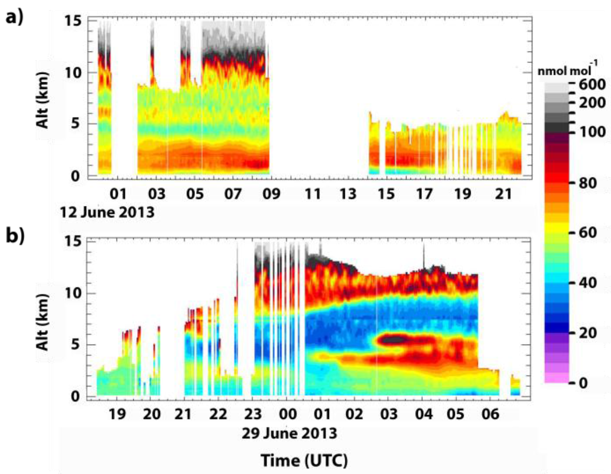
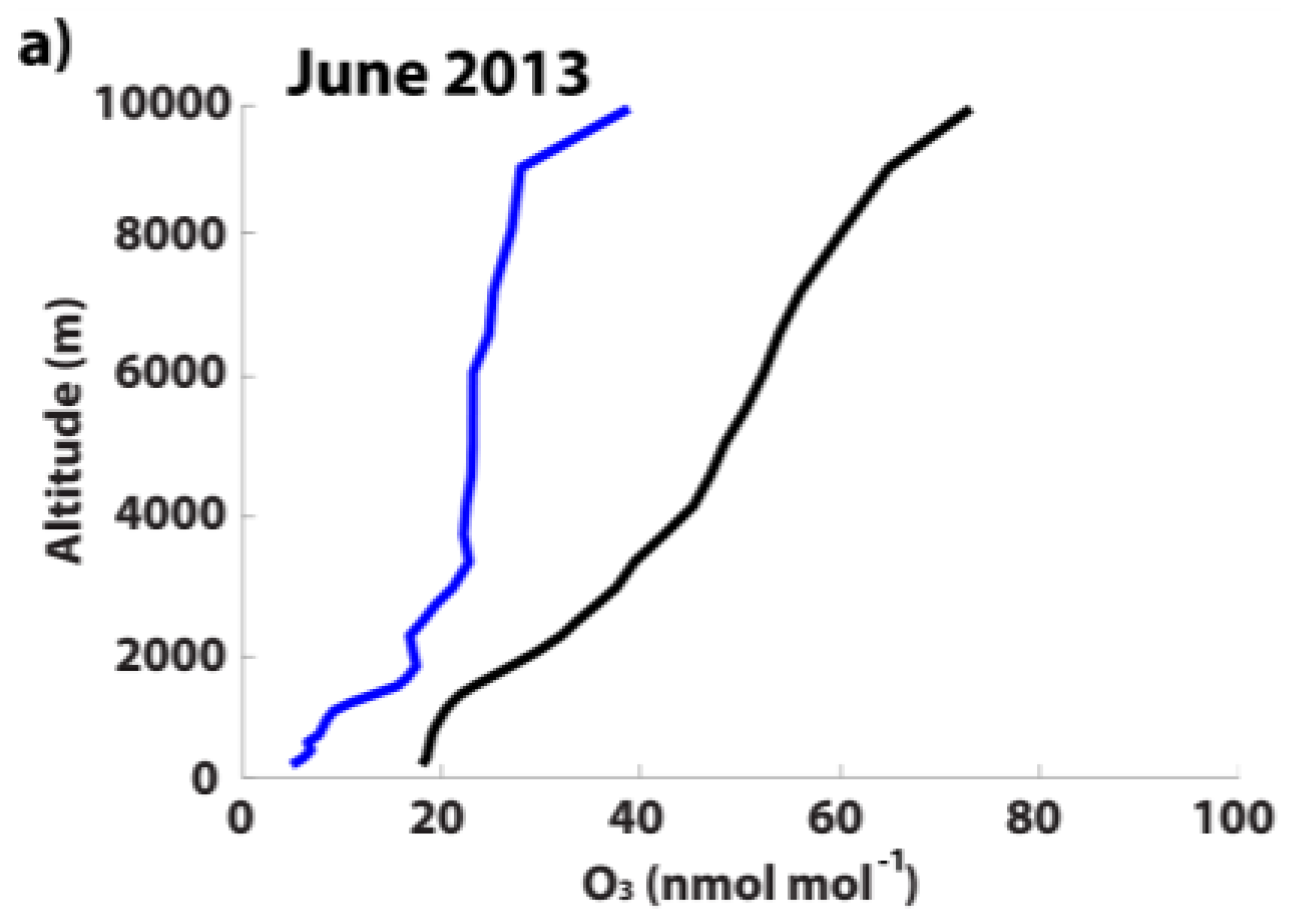
3.1. TOLNet Observations of Enhanced O3 during June 2013

TOLNet observations were analyzed for the entire month of June 2013 and two O3 enhancement cases on 12 and 29 June 2013 were chosen for model evaluation and source apportionment quantification. Figure 1 shows curtain plots of TOLNet observed O3 mixing ratios on 12 June 2013 between 00 and 22 UTC and on 28 June 2013 at 18 UTC to 29 June 2013 at 07 UTC (Central Daylight Time (CDT) = UTC − 5 h). The first case study from 12 June 2013 captured a nocturnal O3 enhancement which occurred near the surface. This study focuses on the time in which the nocturnal O3 enhancement increased from ~65 nmol mol−1 to ~90 nmol mol−1 from 02 to 08 UTC (11 June—09pm to 12 June—03am CDT) (Figure 1a). The second case study is from 29 June 2013 when between 01 and 05 UTC (28 June—08pm to 29 June—12am CDT) a large O3 enhancement layer between ~3 and 6 km above ground level was observed. Ozone mixing ratios during this time reached values of 80 to >100 nmol mol−1 between 03 and 04 UTC (10–11pm CDT). These two case studies were chosen due to the large O3 mixing ratios observed and to evaluate enhancement layers near the surface and in the free troposphere. These events provide a unique opportunity to study sources and transport processes which impact O3 lamina during the summer at different vertical locations in the troposphere of the southeast US.
Figure 2 shows the comparison of GEOS-Chem-predicted and TOLNet observations of vertically resolved O3 averaged between 02 and 08 UTC on 12 June 2013 and 01 to 05 UTC on 29 June 2013. The time-period on 12 June 2013 was selected as TOLNet observations indicated the largest enhancement occurred during these times (see Figure 1a) and the model displayed the relative ability to capture the observed O3 vertical profile (Figure 2a). While the model displays a noticeable negative bias below ~3 km, the model does capture the enhancement occurring at this time and the general pattern of vertically-resolved O3 observed by TOLNet (correlation coefficient (R) = 0.35). Compared to monthly-average model-predicted vertical O3 profiles, the model predicted a nocturnal O3 enhancement of ~10–20 nmol mol−1 below 3 km on 12 June 2013 between 02 and 08 UTC. When comparing the temporally-averaged vertical profile predicted by GEOS-Chem to TOLNet observations the overall normalized mean bias (NMB) was ~−18% between 02 and 08 UTC, primarily driven by the low bias below 3 km.
Figure 2b shows temporally-averaged TOLNet and GEOS-Chem-predicted vertical O3 profiles from 01 to 05 UTC on 29 June 2013. Similar to the case study on 12 June 2013, this time was selected in order to evaluate the largest O3 enhancement occurring on this day and the model displaying the relative ability to reproduce the enhancement layer. From Figure 2b it is clear that GEOS-Chem once again displays a negative bias (NMB = −11.6%), however, is able to reproduce the large enhancement layer occurring between 3 and 6 km. Compared to monthly-average model-predicted O3 values, the model predicted an O3 enhancement between 3 and 6 km of ~10–20 nmol mol−1 on 29 June 2013 between 01 and 05 UTC. The model does appear to display a large overestimation of O3 above 6 km leading to lower correlation values (R = 0.13) between the model and TOLNet observations, but overall is able to reproduce the vertical O3 profile occurring at these times.
Due to the fact that the model reproduces the occurrence of the nocturnal O3 enhancement layer on 12 June and the elevated O3 enhancement lamina on 29 June (and the general pattern of vertical profiles of O3 measured by TOLNet) provides confidence in using the model to evaluate sources impacting TOLNet observations during these times. In order to further determine the ability of the model to simulate O3, and precursor species, during the entire month of June 2013 in the southeast US, GEOS-Chem predictions were evaluated using ground-based and airborne in situ data (see Section 3.2).

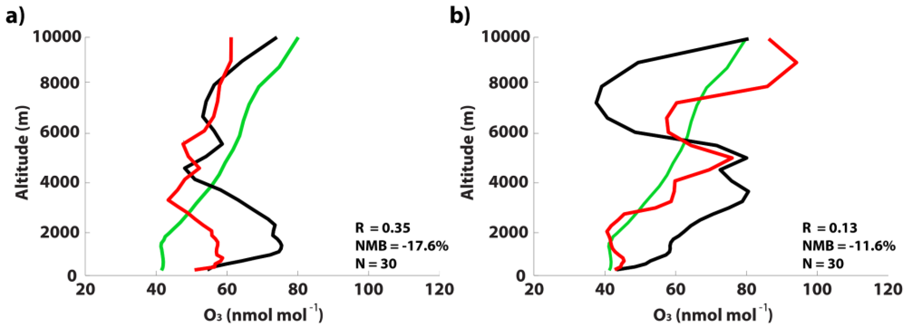
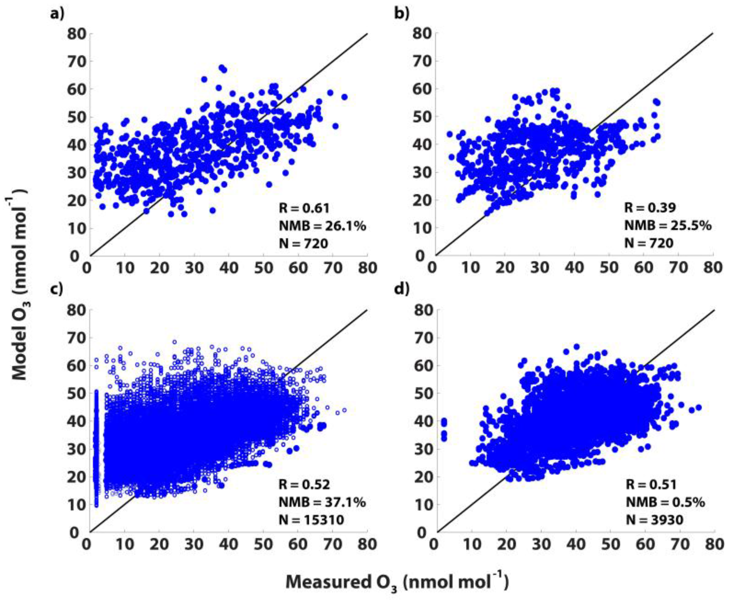
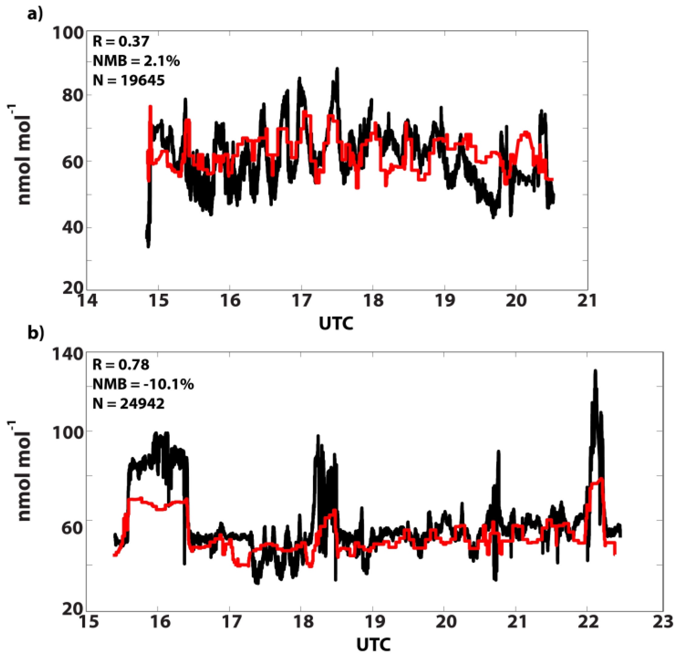
3.2. GEOS-Chem Evaluation

In order to evaluate the ability of GEOS-Chem to reproduce the spatio-temporal variability of O3 occurring in the southeast US, we compare model predictions to surface data from the SEARCH Network and EPA AQS. Figure 3 shows the comparison of hourly-averaged GEOS-Chem-predicted O3 and observations from the BHM and CTR SEARCH Networks in Alabama and all EPA AQS stations in Alabama with data available for all of June 2013 (15 total stations). When comparing the model to surface measurement data at all hours of the day (Figure 3a–c) statistical analysis shows that the model demonstrates relatively good correlations (R = 0.39 to 0.61) and a consistent high bias (NMB = 25.5% to 37.1%). During the model evaluation, time-series analysis clearly demonstrated that this high bias was primarily caused by the model over-predicting the very low night-time O3 values measured at the surface (often well below 10 nmol mol−1). Figure 3d shows that when removing night-time measurement data (only comparing the model to EPA AQS measurements taken between 17 and 22 UTC (12 to 05pm CDT)) the model NMB was reduced to <1%. This result indicates that some transport, chemical, or depositional process occurring during the night is not well captured in GEOS-Chem at the surface layer. However, when the model is compared to the TOLNet observations of the nocturnal near surface O3 enhancement evaluated during this study (Figure 2a) it is shown that the model captures the surface-level O3 mixing ratios and the magnitude of O3 above the large enhancement (>3 km). Figure 4 shows the comparison of airborne measurements of O3 taken on NOAA P3 flights during SENEX and GEOS-Chem predictions on 12 and 29 June 2013 (days in which TOLNet observations of O3 enhancement occurred, flight tracks displayed in Figure S1). During both flights the model demonstrates a relatively strong ability to capture the magnitudes (NMB = −10% to 2.1%) and spatio-temporal variability of measured O3 (R = 0.37 to 0.78). The comparison to airborne data suggests that the model may better reproduce O3 aloft compared to surface level mixing ratios. This is an important finding due to the fact the model is applied in this study to evaluate O3 lamina measured by TOLNet above the surface. Overall, the fact that GEOS-Chem-predicted vertically distributed O3 in the southeast US compared relatively well to in situ data obtained during SENEX flights provides confidence in applying GEOS-Chem to evaluate source attribution of TOLNet O3 observations.
To determine the capability of the model to reproduce the magnitudes and statio-temporal variability of O3 precursor species during the days of the two case studies, we compare predicted values of CO, NOx, and ISOP to P3 data. SENEX measurements was chosen as the primary source of data for this portion of the model evaluation due to the fact it provides measurement data throughout the troposphere and contains information of all precursor species. Table 1 illustrates this model evaluation during the two P3 flights on 12 and 29 June 2013. From this table it can be seen that the model predicts CO mixing ratios that were highly correlated (R > 0.75) with small low biases (NMB = −21%–−23%) compared to P3 measurement data over the southeast US. When evaluating NO2 predictions by GEOS-Chem, the model displays moderate correlation (R = 0.3–0.6) and small low biases (NMB = −3%–−19%). Lower correlation (R = 0.2–0.4) and positive biases (NMB = 24%–56%) were determined when comparing GEOS-Chem NO predictions to the P3 data. Finally, model-predicted ISOP values were generally higher compared to measurements (NMB = 60%–85%) with high correlation (R = ~0.6) during both P3 flights over the southeast US. Overall, when compared to airborne measurement data over the southeast US, small to moderate biases in model-predicted O3 precursor species were calculated. These model biases are similar in magnitude to other modeling studies in this region (e.g., [29,34]) providing further confidence in applying GEOS-Chem to evaluate source attribution of TOLNet O3 observations.

3.3. Sources of O3 Measured by TOLNet

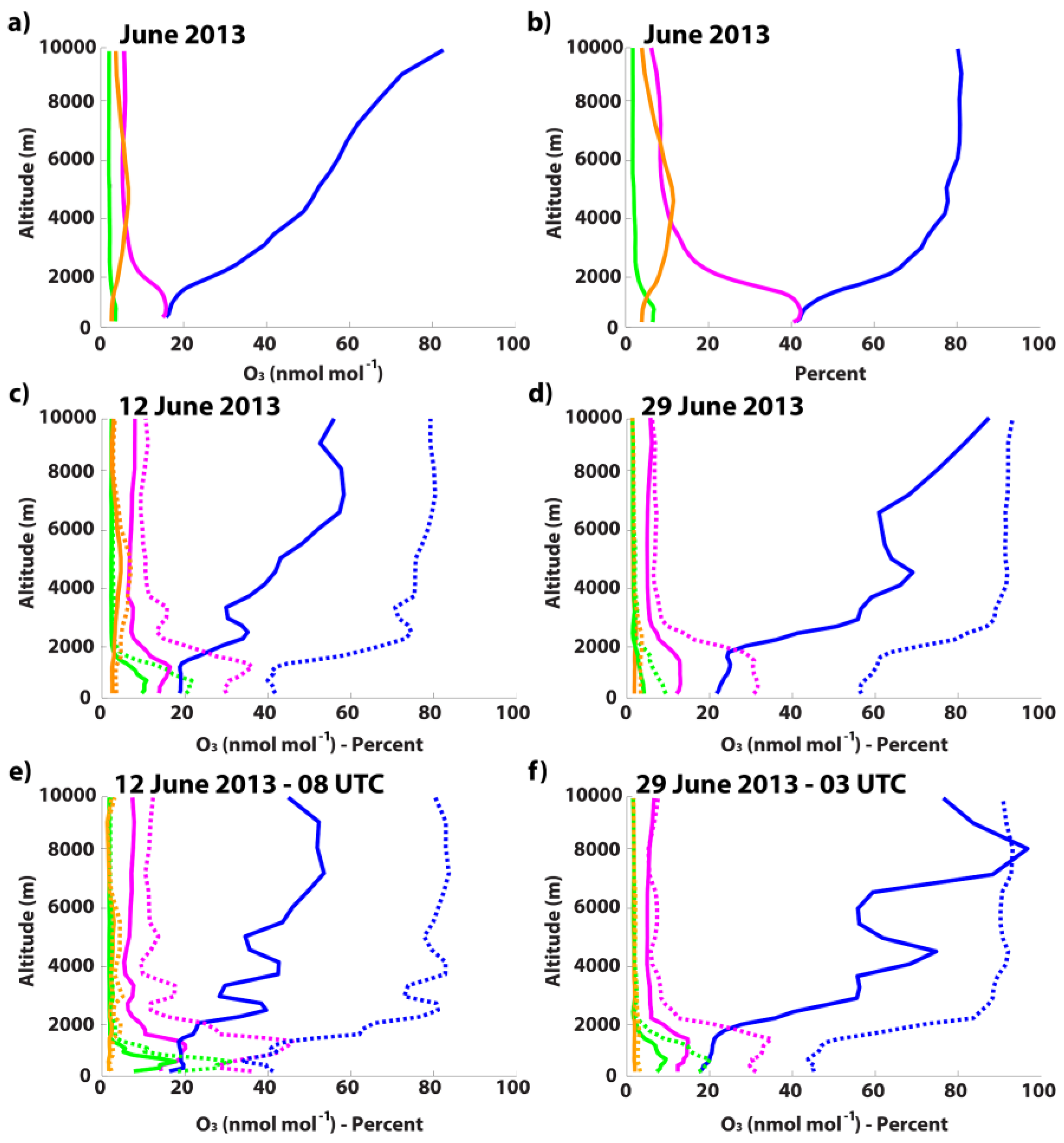
3.3.1. Monthly-Averaged Source Attribution during June 2013
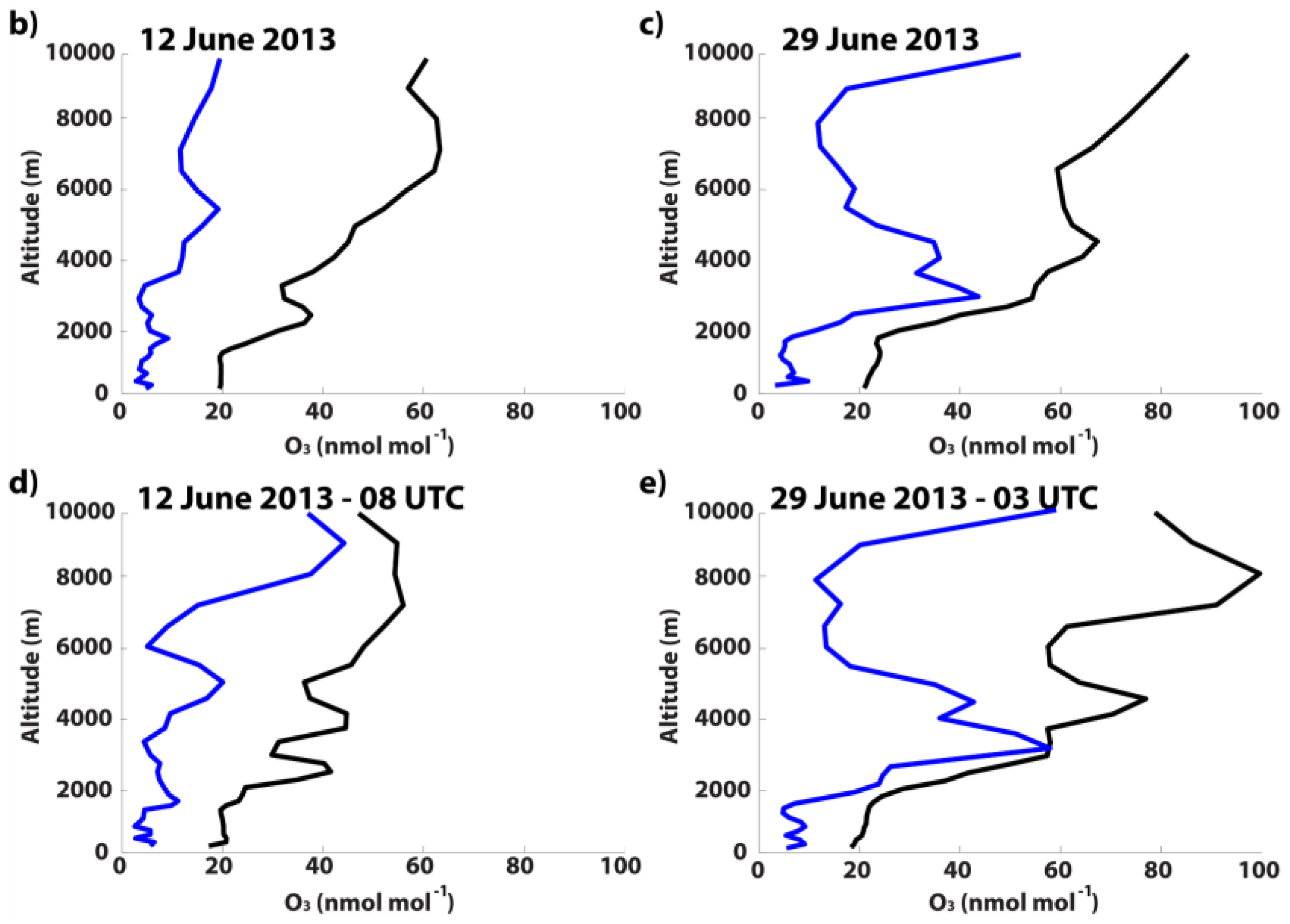
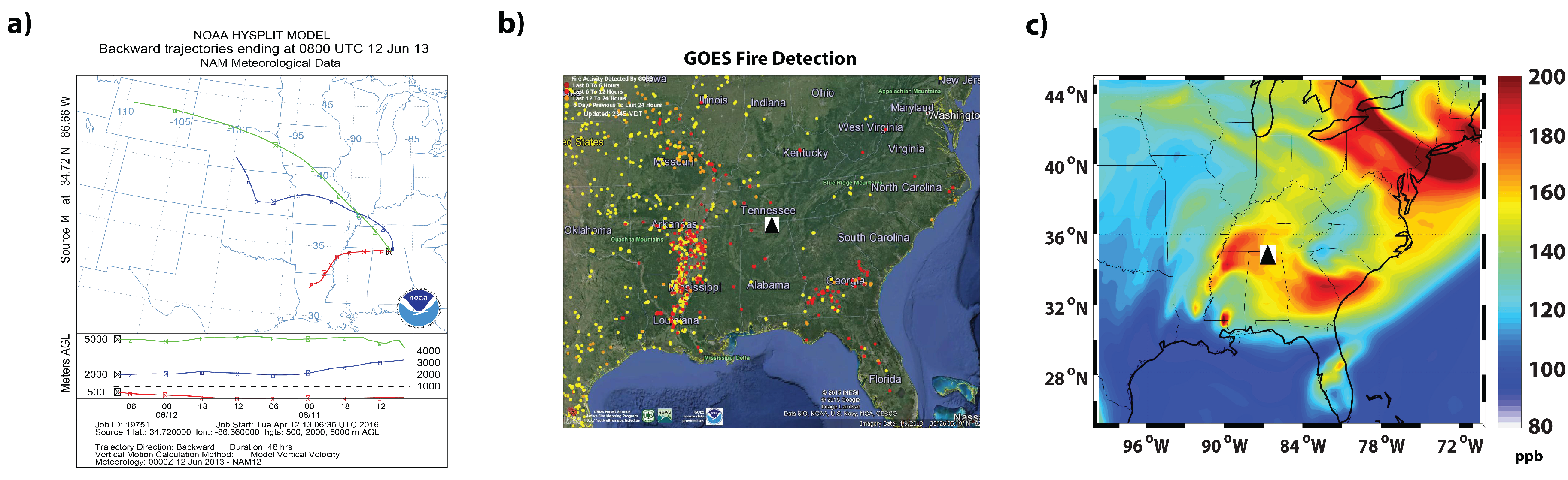
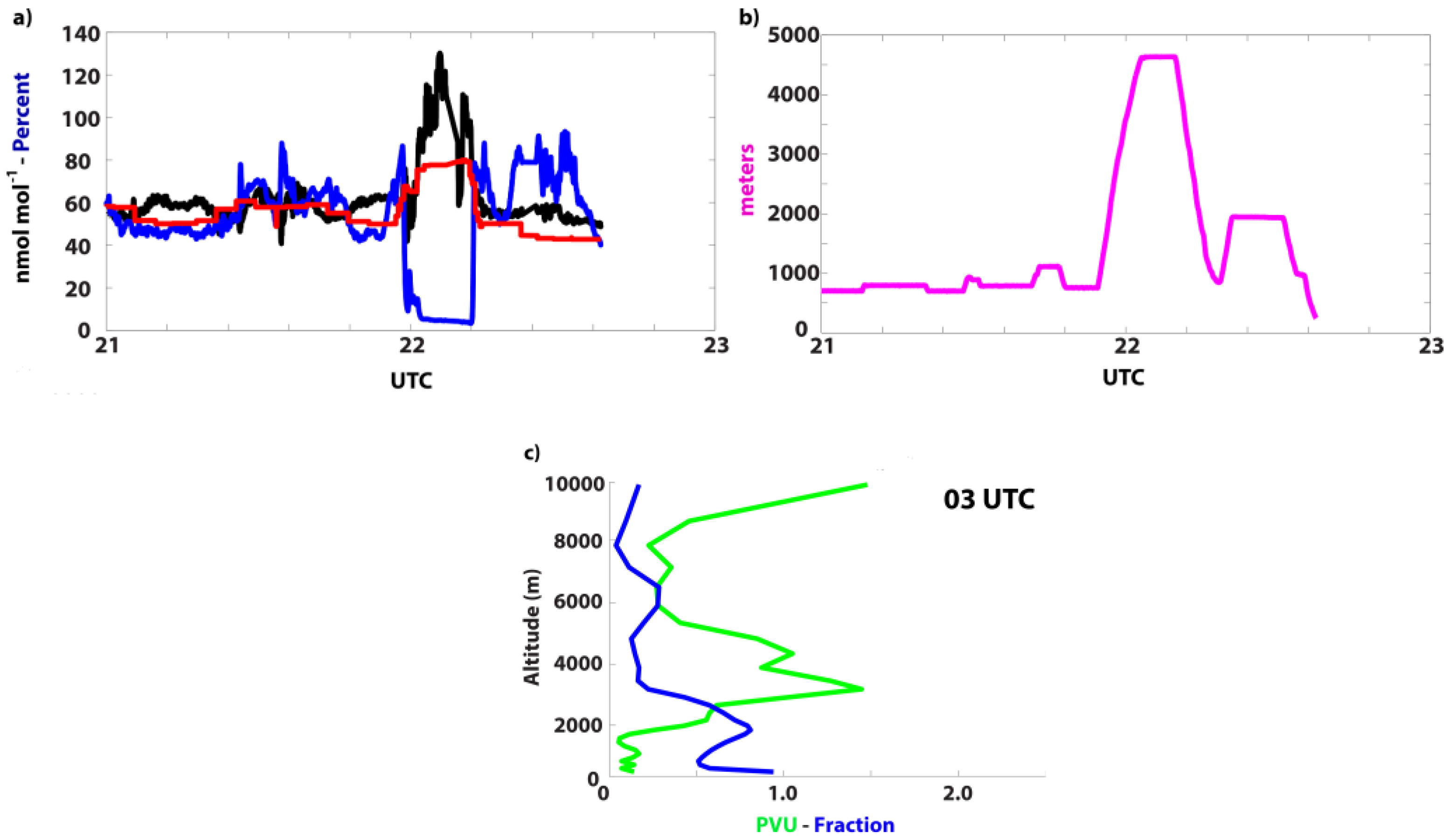
In order to determine the emission sources and transport pathways that were contributing to total O3 over the UAH TOLNet site during June 2013, “brute force” sensitivity simulations were conducted to quantify O3 production due to North American anthropogenic emissions, wildfires, lightning NOx, and long-range/stratospheric transport. To evaluate the contribution from individual emission sources and transport processes to total O3 during summer months, we compute source specific O3 magnitudes and the percent contribution to total O3 for the entire month of June 2013. Monthly-averaged O3 source attribution is shown in Figure 5a,b and from this figure it can be seen that near the surface (<2 km) anthropogenic emissions and long-range transport (long-range tropospheric + stratospheric) O3 make up the majority of model predicted O3. The source attribution of total O3 aloft (>3 km) is predominantly contributed from long-range/stratospheric transport, lightning NOx, and anthropogenic emissions.
Table 2 shows the quantified model-predicted contribution from individual sources at the UAH TOLNet site for the entire month of June 2013 and the two case studies evaluated during this study (illustrated in Figure 5). The source-specific O3 magnitude and percent contribution are shown for monthly-averaged model predictions, daily-averaged values for 12 and 29 June 2013, and hourly-averaged values for 08 UTC (03am CDT) on 12 June 2013 (between 0–1 km and 0–3 km) and 03 UTC (10pm CDT) on 29 June 2013 (between 3 and 6 km). Monthly-averaged source contribution of total O3 near the surface is predominantly from anthropogenic emissions (~36% and 44% below 3 km and 1 km, respectively) and long-range/stratospheric transport (~56% and 47% below 3 km and 1 km, respectively). From Table 2 it can also be seen that total O3 between 3–6 km for the month of June 2013 is primarily from long-range/stratospheric transport (~78%), anthropogenic emissions (~12%), and lightning NOx (~9%). In order to estimate the amount of long-range transport O3 that is from only stratospheric transport we plot the vertical profiles of total long-range transport O3 (long-range tropospheric + stratospheric) and just stratospheric sources (based on GEOS-5 PVU) separately (see Figure 6). This figure shows the amount of total long-range transport O3 and just stratospheric O3 over the UAH TOLNet site for the entire month of June 2013, daily-averaged values for 12 and 29 June 2013, and hourly-averaged values for 08 UTC on 12 June 2013 and 03 UTC on 29 June 2013. From this figure it is shown that above ~2 km during the month of June 2013, ~30%–80% of long-range transport O3 was from stratospheric transport (this estimate assumes that stratospheric O3 calculated from GEOS-5 PVU values is representative of stratospheric impact on total long-range transport O3 from GEOS-Chem).

3.3.2. 12 June 2013

TOLNet observations on 12 June 2013 captured a nocturnal O3 enhancement layer near the surface between 02 and 08 UTC. To determine the emission sources and transport processes contributing to the enhancement measured by TOLNet on 12 June 2013, “brute force” sensitivity simulations were conducted. Sensitivity studies were conducted to determine the source attribution of O3 for the entire day and during the hour in which largest enhancements were measured (08 UTC). The results of these sensitivity studies are presented in Figure 5c,e, respectively. From this figure it can be seen that the model predicted anthropogenic emission sources and long-range transport O3 to be the main sources contributing to O3 near the surface on 12 June 2013 with values ranging between 15 and 20 nmol mol−1. When near-surface O3 enhancements were measured to be at a maximum at 08 UTC, the model predicts a large impact from wildfire emissions with values reaching >15 nmol mol−1 (below 1.5 km) and anthropogenic emissions contribution had a daily maximum during these night-time hours. The model predicts a maximum daily contribution from anthropogenic emissions during the night-time hours (between 02 and 08 UTC) instead of the afternoon hours on 12 June 2013. GEOS-5 meteorological data indicates that a weak low level jet (LLJ) may have been occurring as the westerly wind component (U wind) below 2 km increased from <5 m·s−1 at 00 UTC (07pm CDT) to >10 m·s−1 at 09 UTC (04am CDT). LLJs occur frequently in the southeast US and can transport O3 and precursor species from urban regions to rural areas in the late afternoon and night-time hours resulting in nocturnal O3 enhancements (e.g., [17]). Long-range/stratospheric sources contributed O3 mixing ratios near the surface which were similar to monthly-averaged values (~20 nmol mol−1). Using the methods of [45] to determine “pure” stratospheric O3 (see Section 2.4) which separates O3 values associated with photochemically generated tropospheric values (applying model-predicted PVU and O3:PV ratios) and those strictly contributed from stratospheric intrusions, it was determined this contribution from long-range/stratospheric sources was likely primarily from the long-range transport of tropospheric O3 and precursor species as model-predicted stratospheric O3 at 08 UTC on 12 June 2013 was predicted to only be “pure” above ~9 km.
Wildfires are a major source of NOx and VOCs and thus have substantial impact on O3 enhancement events (e.g., [49]). GEOS-Chem simulated large O3 mixing ratios due to wildfire emissions, especially at 08 UTC (see Figure 5e) on 12 June 2013. From Table 2 it can be seen that wildfire emissions on average contribute ~2 nmol mol−1 of O3 (~6% of total) below 1 km in June 2013. During the large nocturnal O3 enhancement measured by TOLNet the model predicts a contribution of ~11 nmol mol−1 (ranging from 10 to 20 nmol mol−1) which is ~23% of total O3. This clearly demonstrates that the model predicts an enhancement from wildfire emissions occurring in the southeast US during this time period. Simple back-trajectories simulated using the Hybrid Single Particle Lagrangian Integrated Trajectory (HYSPLIT) model driven with 12 km North American Mesoscale Forecast System (NAM) meteorological data are shown in Figure 7a. These trajectory calculations were initiated at 08 UTC on 12 June 2013 at vertical heights of 500, 2000, and 5000 m above ground level and run backwards in time for 48 h. From this figure it is clear that minimal vertical mixing occurred in the air mass of the lowest layer (parcel started at 500 m above ground level) and remains near the surface as it was transported over the areas of active burning in Mississippi, Arkansas, and Louisiana observed by the 4 km Geostationary Operational Environmental Satellite (GOES) fire detection data on 12 June 2013 (see Figure 7b). The backtrajectories for air parcels initiated in the PBL calculated by HYSPLIT are in agreement with Weather Research and Forecasting FLEXible PARTicle (WRF-FLEXPART) dispersion model backtrajectories calculated for SENEX flights [50] occurring later in the day on 12 June 2013. Furthermore, GEOS-Chem predicted elevated mixing ratios of CO below 2 km between 00 and 08 UTC (7pm–03am CDT) on 12 June 2013 over the UAH TOLNet station and upwind over the region of large fire activity (see Figure 7c). Finally, P3 airborne measurements on the afternoon of 12 June 2013 indicate elevated CO and BC concentrations aloft. Measured CO concentrations above the surface reached values >200 nmol mol−1 and BC concentrations were highly variable and reached values between 400 and 500 ng·m−3 which is nearly a factor of 2 larger compared to averaged surface-level concentrations measured by IMPROVE sites in the southeast US during the summer of 2013 [51].

3.3.3. 29 June 2013

TOLNet observations on 29 June 2013 captured a large O3 enhancement layer from 3 to 6 km above ground level between 01 and 05 UTC. To determine the emission sources and transport processes contributing to the enhancement measured by TOLNet on 29 June 2013, “brute force” sensitivity simulations were conducted. From Figure 5d,f it is shown that long-range/stratospheric transport likely had a significant impact on the O3 enhancement measured by TOLNet on 29 June 2013 between 01 and 05 UTC from 3 to 6 km. From Table 2 it can be seen that long-range/stratospheric transport was predicted by the model to be larger on 29 June 2013, and during the time of largest O3 enhancement at 03 UTC, compared to monthly-averaged values. During the time of largest observed enhancements, the model predicts long-range/stratospheric transport to contribute >20 nmol mol−1 more O3 compared to average conditions. While long-range/stratospheric transport is typically contributing the majority of O3 between 3–6 km over the UAH TOLNet site (~78% on average), at 03 UTC on 29 June 2013 long-range/stratospheric transport contributed >90% of total O3 in the enhancement layer.
Figure 6c,e show the contribution of just stratospheric O3 to total long-range transport O3 for 29 June 2013 and at 03 UTC on this day. From this figure it is shown that stratospheric transport was potentially contributing largely to the enhancement layer at 03 UTC compared to monthly-averages. Using GEOS-5 PVU values it is estimated that between 3–6 km stratospheric transport contributed up to 60 nmol mol−1 of O3 and was up to ~100% of total long-range transport O3 between 3 and 5 km with less influence between 5 and 6 km. Applying the methods of [45] to determine “pure” stratospheric O3, it was determined that the stratospheric O3 between 2 and 5 km was “pure” at this time, thus likely associated with a stratospheric intrusion. Figure 8 shows airborne measurements of O3 and relative humidity (RH) during P3 flights and GEOS-Chem-predicted O3 values. These airborne measurements were taken during P3 flights which occurred later in the day on 29 June 2013 in close proximity (just downwind) of the UAH TOLNet site and this measurement data captured the large O3 lamina between 3 and 6 km. Furthermore, the measurement data shows that the large O3 values were occurring in a very dry (RH < 5%) air mass with CO mixing ratios <100 nmol mol−1 indicating the influence of stratospheric air. The P3 measurement data agrees with GEOS-5 model predictions at 03 UTC of PVU and RH values which indicate PVU values >1.0 co-located with RH values <15% between 3 and 6 km (see Figure 8c). In addition to model and measurement results from this study, Global Forecast System (GFS)-FLEXPART simulations conducted to support the SENEX campaign also suggest that enhanced stratospheric O3 occurred on 29 June 2013 between 3 and 6 km [52].

4. Conclusions

As the EPA implements legislation which reduces NAAQS values for surface O3, it becomes increasingly important to understand the emission sources of precursor species, transport pathways, and chemical processes resulting in elevated O3 mixing ratios. During this study, we apply TOLNet lidar observations, surface and airborne in situ data, and model simulations to better understand the emission sources and transport processes impacting O3 mixing ratios in the southeast US. This study focuses on O3 enhancement lamina measured by the UAH TOLNet lidar system during June 2013. This location is representative of southeast US air quality as it is impacted by numerous anthropogenic and natural emission sources of precursor species (e.g., fossil fuel combustion, vehicles, wildfires, lightning, soils, vegetation, etc.) and transport pathways (e.g., local, long-range/inter-continental, stratospheric, etc.). To identify and quantify the sources impacting O3 enhancement lamina measured by the UAH TOLNet, we apply baseline GEOS-Chem model simulations and “brute force” sensitivity simulations during June 2013. This study focused on two case studies: (1) a nocturnal O3 enhancement layer near the surface on 12 June 2013 and (2) a large O3 enhancement layer between ~3 and 6 km on 29 June 2013. These two events provided a unique opportunity to study sources and transport processes which impact O3 enhancements in the southeast US at different times and vertical locations in the troposphere.
To determine the ability of GEOS-Chem to capture the mixing ratios of O3 and precursor species in the southeast US, the model was evaluated using SEARCH and EPA AQS surface in situ data and airborne measurements from P3 flights conducted during SENEX. Evaluating the model with surface measurement data of O3 demonstrated that the model had relatively good correlations (R = 0.39 to 0.61) and a consistent high bias (NMB = 25.5% to 37.1%) compared to observations. Time-series analysis indicated that the model over-prediction was primarily occurring during night-time hours near the surface. The model proved to be able to reproduce O3 mixing ratios measured during P3 flights on 12 and 29 June 2013 above the surface in varying location of the southeast US. During both flights the model captured the magnitudes (NMB = −10% to 2.1%) and spatio-temporal variability of measured O3 (R = 0.37 to 0.78). Ozone precursors species (CO, NOx, and ISOP) predicted by GEOS-Chem were also evaluated using P3 measurements during flights on 12 and 29 June 2013. During these flights the model demonstrated the general ability to replicate measurements of CO, NOx, and ISOP over the southeast US. Overall, the model compared moderately well with ground-based measurements and had better agreement with airborne in situ data which provided confidence this model could be applied for estimating source apportionment of the O3 measured by the UAH TOLNet.
Sensitivity simulations were conducted for the entire month of June 2013 and for the two case studies on 12 and 29 June 2013 to quantify O3 production due to North American anthropogenic emissions, wildfires, lightning NOx, and long-range/stratospheric transport. Monthly-averaged O3 source attribution demonstrated in this study shows that on average near the surface (<2 km) anthropogenic emissions and long-range/stratospheric O3 make up the majority of model predicted O3. Monthly-averaged source attribution of total O3 aloft (>3 km) is predominantly contributed from long-range/stratospheric transport, lightning NOx, and anthropogenic emissions.
During the time periods of the two case studies, noticeable differences in O3 source attribution were predicted compared to monthly-averaged values. On 12 June 2013 the near-surface O3 enhancement measured by TOLNet between 02 and 08 UTC, was predicted by the model to have large impact from wildfire emissions with values reaching >15 nmol mol−1 (below 1.5 km). HYSPLIT back-trajectories, GOES fire detection data, and P3 airborne measurement data evaluated during this study further indicate that wildfire emission were likely impacting near-surface air quality and O3 mixing ratios within this O3 enhancement layer. Furthermore, the model predicted that anthropogenic emissions had daily maximum contribution (>15 nmol mol−1) during these night-time hours. When evaluating GEOS-5 meteorological data it is suggested that a weak LLJ could have contributed to this nocturnal enhancement of anthropogenic impact. When evaluating model-predicted source attribution during the case study for the elevated (3–6 km) O3 lamina on 29 June 2013 between 01 and 05 UTC, it was determined that long-range/stratospheric sources were the major contributor to this enhancement. Separating stratospheric sources from total long-range transport O3 and applying methods to calculate “pure” stratospheric air suggests that the majority of the O3 enhancement on this day was from a stratospheric intrusion occurring in the southeast US. Measurement data from a P3 flight on 29 June 2013 agree with the model-predicted source attribution from this study, clearly indicating that the O3 lamina between 3 and 6 km was associated with very dry (RH <5%) and clean (CO <100 nmol mol−1) air associated with a stratospheric intrusion.
This study emphasizes the fact that numerous emission sources and transport pathways control tropospheric O3 in the southeast US during the summer. In particular it is shown that there is large variability in the magnitude and source attribution of O3 throughout the vertical extent of the troposphere. Finally, in order to better understand emission sources, transport processes, and chemical reactions that control the source attribution of O3 in different vertical levels of the troposphere, it is important to apply numerous sources of measurement data (e.g., surface-based and airborne), remote-sensing observations (e.g., ground-based lidar profiles), and model simulations.

Supplementary Materials

The following are available online at www.mdpi.com/2073-4433/7/8/108/s1. Figure S1: Flight tracks of NOAA P3 measurements during the SENEX field campaign on (a) 12 June 2013 and (b) 29 June 2013 overlaid on Google Earth; Figure S2: GEOS-Chem-predicted monthly-averaged O3 (black line, nmol mol−1), summation of source attributed O3 (red line, nmol mol−1), and the percent difference between baseline and summation of source attributed O3 (blue line, %) over the UAH TOLNet site during June 2013.

Acknowledgments

This work is supported by the TOLNet program developed by NASA’s Science Mission Directorate. Matthew Johnson would also like to thank Daniel Jacob, Katie Travis, and the Harvard University Atmospheric Chemistry Modeling Group for providing the base model GEOS-Chem used during our research. We would also like to thank the SENEX science, instrument, and aircraft teams, with particular thanks to Ilana Pollack and Thomas Ryerson (O3, NOx), Joshua Schwarz (BC), John S. Holloway (CO), and Martin Graus (Isoprene) for specific trace gas and aerosol data. Resources supporting this work were provided by the NASA High-End Computing (HEC) Program through the NASA Advanced Supercomputing (NAS) Division at NASA Ames Research Center. All the authors express gratitude to the support from NASA’s Earth Science Division at Ames Research Center. Finally, the views, opinions, and findings contained in this report are those of the authors and should not be construed as an official NASA or United States Government position, policy, or decision.

Author Contributions

Matthew S. Johnson and Michael J. Newchurch conceived the overall research topic and obtained funding to support the work. Data sources, materials, and evaluation techniques used during the study were developed by Matthew S. Johnson, Shi Kuang, and Lihua Wang. All model simulations and data evaluation were performed by Matthew S. Johnson. Matthew S. Johnson wrote the manuscript with the assistance of significant editorial and scientific improvements from all authors of the manuscript.

Conflicts of Interest

The authors declare no conflict of interest.

References

  1. U.S. Environmental Protection Agency. Air Quality Criteria for Ozone and Related Photochemical Oxidants (2006 Final); EPA/600/R-05/004aF-cF; U.S. Environmental Protection Agency: Washington, DC, USA, 2006.
  2. Worden, H.M.; Bowman, K.W.; Worden, J.R.; Eldering, A.; Beer, R. Satellite measurements of the clear-sky greenhouse effect from tropospheric ozone. Nat. Geosci. 2008, 1, 305–308. [Google Scholar] [CrossRef]
  3. U.S. Environmental Protection Agency. National Ambient Air Quality Standards for Ozone—Final Rule; Federal Register 80; U.S. Environmental Protection Agency: Washington, DC, USA, 2015.
  4. Fiore, A.M.; Jacob, D.J.; Liu, H.; Yantosca, R.M.; Fairlie, T.D.; Li, Q. Variability in surface ozone background over the United States: Implications for air quality policy. J. Geophys. Res. Atmos. 2003. [Google Scholar] [CrossRef]
  5. Vingarzan, R. A review of surface ozone background levels and trends. Atmos. Environ. 2004, 38, 3431–3442. [Google Scholar] [CrossRef]
  6. Lefohn, A.S.; Wernli, H.; Shadwick, D.; Limbach, S.; Oltmans, S.J.; Shapiro, M. The importance of stratospheric-tropospheric transport in affecting surface ozone concentrations in the western and northern tier of the United States. Atmos. Environ 2011, 45, 4845–4857. [Google Scholar] [CrossRef]
  7. Lin, M.; Fiore, A.M.; Cooper, O.R.; Horowitz, L.W.; Langford, A.O.; Levy, H.; Johnson, B.J.; Naik, V.; Oltmans, S.J.; Senff, C.J. Springtime high surface ozone events over the western United States: Quantifying the role of stratospheric intrusions. J. Geophys. Res. 2012, 117. [Google Scholar] [CrossRef]
  8. Yates, E.L.; Iraci, L.T.; Roby, M.C.; Pierce, R.B.; Johnson, M.S.; Reddy, P.J.; Tadić, J.M.; Loewenstein, M.; Gore, W. Airborne observations and modeling of springtime stratosphere-to-troposphere transport over California. Atmos. Chem. Phys. 2013, 13, 12481–12494. [Google Scholar] [CrossRef]
  9. Zhang, L.; Jacob, D.J.; Yue, X.; Downey, N.V.; Wood, D.A.; Blewitt, D. Sources contributing to background surface ozone in the US Intermountain West. Atmos. Chem. Phys. 2014, 14, 5295–5309. [Google Scholar] [CrossRef]
  10. Lin, M.; Fiore, A.M.; Horowitz, L.W.; Langford, A.O.; Oltmans, S.J.; Tarasick, D.; Reider, H.E. Climate variability modulates western US ozone air quality in spring via deep stratospheric intrusions. Nat. Commun. 2015, 6. [Google Scholar] [CrossRef] [PubMed]
  11. Hidy, G.M.; Blanchard, C.L.; Baumann, K.; Edgerton, E.; Tanenbaum, S.; Shaw, S.; Knipping, E.; Tombach, I.; Jansen, J.; Walters, J. Chemical climatology of the southeastern United States. Atmos. Chem. Phys. 2014, 14, 11893–11914. [Google Scholar] [CrossRef]
  12. Pfister, G.G.; Emmons, L.K.; Hess, P.G.; Lamarque, J.-F.; Thompson, A.M.; Yorks, J.E. Analysis of the Summer 2004 ozone budget over the United States using Intercontinental Transport Experiment Ozonesonde Network Study (IONS) observations and Model of Ozone and Related Tracers (MOZART-4) simulations. J. Geophys. Res. 2008, 113. [Google Scholar] [CrossRef]
  13. Hudman, R.C.; Murray, L.T.; Jacob, D.J.; Turquety, S.; Wu, S.; Millet, D.B.; Avery, M.; Goldstein, A.H.; Holloway, J. North American influence on tropospheric ozone and the effects of recent emission reductions: Constraints from ICARTT observations. J. Geophys. Res. 2009, 114. [Google Scholar] [CrossRef]
  14. TOLNet-Tropospheric Ozone Lidar Network. Available online: http://www-air.larc.nasa.gov/missions/TOLNet/ (accessed on 15 July 2015).
  15. Kuang, S.; Burris, J.F.; Newchurch, M.J.; Johnson, S.; Long, S. Differential absorption Lidar to measure subhourly variation of tropospheric ozone profiles. IEEE Trans. Geosci. Remote Sens. 2011, 49, 557–571. [Google Scholar] [CrossRef]
  16. Kuang, S.; Newchurch, M.J.; Burris, J.; Liu, X. Ground-based Lidar for atmospheric boundary layer ozone measurements. Appl. Opt. 2013, 52, 3557–3566. [Google Scholar] [CrossRef] [PubMed]
  17. Kuang, S.; Newchurch, M.J.; Burris, J.; Wang, L.; Buckley, P.; Johnson, S.; Knupp, K.; Huang, G.; Phillips, D. Nocturnal ozone enhancement in the lower troposphere observed by Lidar. Atmos. Environ. 2011, 45, 6078–6084. [Google Scholar] [CrossRef]
  18. Kuang, S.; Newchurch, M.J.; Burris, J.; Wang, L.; Knupp, K.; Huang, G. Stratosphere-to-troposphere transport revealed by ground-based Lidar and ozonesonde at a midlatitude site. J. Geophys. Res. 2012, 117. [Google Scholar] [CrossRef]
  19. Wang, L.; Follette-Cook, M.; Newchurch, M.; Pickering, K.; Pour-Biazar, A.; Kuang, S.; Koshak, W.; Peterson, H. Evaluation of lightning-induced tropospheric ozone enhancements observed by ozone Lidar and simulated by WRF/Chem. Atmos. Environ. 2015, 115, 185–191. [Google Scholar] [CrossRef]
  20. SouthEastern Aerosol Research and Characterization (SEARCH) Network. Available online: http://www.atmospheric-research.com/studies/SEARCH/ (accessed on 20 September 2015).
  21. Environmental Protection Agency—AirData. Available online: https://www3.epa.gov/airquality/airdata/ (accessed on 20 September 2015).
  22. Earth System Research Laboratory—Chemical Sciences Division—SENEX Data. Available online: http://www.esrl.noaa.gov/csd/groups/csd7/measurements/2013senex/ (accessed on 13 January 2016).
  23. Bey, I.; Jacob, D.J.; Yantosca, R.M.; Logan, J.A.; Field, B.; Fiore, A.M.; Li, Q.; Liu, H.; Mickley, L.J.; Schultz, M. Global modeling of tropospheric chemistry with assimilated meteorology: Model description and evaluation. J. Geophys. Res. 2001, 106, 23073–23095. [Google Scholar] [CrossRef]
  24. Lin, S.J.; Rood, R.B. Multidimensional flux form semi-Lagrangian transport schemes. Mon. Weather Rev. 1996, 124, 2046–2070. [Google Scholar] [CrossRef]
  25. Lin, J.-T.; McElroy, M. Impacts of boundary layer mixing on pollutant vertical profiles in the lower troposphere: Implications to satellite remote sensing. Atmos. Environ. 2010, 44, 1726–1739. [Google Scholar] [CrossRef]
  26. Liu, H.; Jacob, D.J.; Bey, I.; Yantosca, R.M. Constraints from 210Pb and 7Be on wet deposition and transport in a global three dimensional chemical tracer model driven by assimilated meteorological fields. J. Geophys. Res. 2001, 106, 12109–12128. [Google Scholar] [CrossRef]
  27. Amos, H.M.; Jacob, D.J.; Holmes, C.D.; Fisher, J.A.; Wang, Q.; Yantosca, R.M.; Corbitt, E.S.; Galarneau, E.; Rutter, A.P.; Gustin, M.S.; et al. Gas-Particle partitioning of atmospheric Hg(II) and its effect on global mercury deposition. Atmos. Chem. Phys. 2012, 12, 591–603. [Google Scholar] [CrossRef]
  28. Wang, Y.H.; Jacob, D.J.; Logan, J.A. Global simulation of tropospheric O3-NOx-hydrocarbon chemistry: 1. Model formulation. J. Geophys. Res. 1998, 103, 10713–10725. [Google Scholar] [CrossRef]
  29. Travis, K.R.; Jacob, D.J.; Fisher, J.A.; Kim, P.S.; Marais, E.A.; Zhu, L.; Yu, K.; Miller, C.C.; Yantosca, R.M.; Sulprizio, M.P.; et al. NOx emissions, isoprene oxidation pathways, vertical mixing, and implications for surface ozone in the Southeast United States. Atmos. Chem. Phys. Discuss. 2016. [Google Scholar] [CrossRef]
  30. Environmental Protection Agency—Air Pollutant Emissions Trends Data. Available online: https://www.epa.gov/air-emissions-inventories/air-pollutant-emissions-trends-data (accessed on 5 August 2015).
  31. Fujita, E.M.; Campbell, D.E.; Zielinska, B.; Chow, J.C.; Lindhjem, C.E.; DenBleyker, A.; Bishop, G.A.; Schuchmann, B.G.; Stedman, D.H.; Lawson, D.R. Comparison of the MOVES2010a, MOBILE6.2, and EMFAC2007 mobile source emission models with on-road traffic tunnel and remote sensing measurements. J. Air Waste Manag. Assoc. 2012, 62, 1134–1149. [Google Scholar] [CrossRef] [PubMed]
  32. Brioude, J.; Angevine, W.M.; Ahmadov, R.; Kim, S.W.; Evan, S.; McKeen, S.A.; Hsie, E.Y.; Frost, G.J.; Neuman, J.A.; Pollack, I.B.; et al. Top-down estimate of surface flux in the Los Angeles Basin using a mesoscale inverse modeling technique: assessing anthropogenic emissions of CO, NOx and CO2 and their impacts. Atmos. Chem. Phys. 2013, 13, 3661–3677. [Google Scholar] [CrossRef]
  33. Anderson, D.C.; Loughner, C.P.; Diskin, G.; Weinheimer, A.; Canty, T.P.; Salawitch, R.J.; Worden, H.M.; Fried, A.; Mikoviny, T.; Wisthaler, A.; et al. Measured and modeled CO and NOy in DISCOVER-AQ: An evaluation of emissions and chemistry over the eastern US. Atmos. Environ. 2014, 96, 78–87. [Google Scholar] [CrossRef]
  34. Canty, T.P.; Hembeck, L.; Vinciguerra, T.P.; Anderson, D.C.; Goldberg, D.L.; Carpenter, S.F.; Allen, D.J.; Loughner, C.P.; Salawitch, R.J.; et al. Ozone and NOx chemistry in the eastern US: Evaluation of CMAQ/CB05 with satellite (OMI) data. Atmos. Chem. Phys. 2015, 15, 10965–10982. [Google Scholar] [CrossRef]
  35. Darmenov, A.S.; da Silva, A. The Quick Fire Emissions Dataset (QFED): Documentation of Versions 2.1, 2.2 and 2.4. Available online: https://gmao.gsfc.nasa.gov/pubs/docs/Darmenov796.pdf (accessed on 19 August 2016).
  36. Murray, L.T.; Jacob, D.J.; Logan, J.A.; Hudman, R.C.; Koshak, W.J. Optimized regional and interannual variability of lightning in a global chemical transport model constrained by LIS/OTD satellite data. J. Geophys. Res. 2012, 117. [Google Scholar] [CrossRef]
  37. Hudman, R.C.; Jacob, D.J.; Turquety, S.; Leibensperger, E.M.; Murray, L.T.; Wu, S.; Gilliland, A.B.; Avery, M.; Bertram, T.H.; Brune, W.; et al. Surface and lightning sources of nitrogen oxides over the United States: Magnitudes, chemical evolution, and outflow. J. Geophys. Res. 2007, 112. [Google Scholar] [CrossRef]
  38. McLinden, C.A.; Olsen, S.C.; Hannegan, B.; Wild, O.; Prather, M.J.; Sundet, J. Stratospheric ozone in 3-D models: A simple chemistry and the cross-tropopause flux. J. Geophys. Res. 2000, 105, 14653–14665. [Google Scholar] [CrossRef] [Green Version]
  39. Hsu, J.; Prather, M.J.; Wild, O. Diagnosing the stratosphere-to-troposphere flux of ozone in a chemistry transport model. J. Geophys. Res. 2005, 110. [Google Scholar] [CrossRef] [Green Version]
  40. Ott, L.E.; Duncan, B.N.; Thompson, A.M.; Diskin, G.; Fasnacht, Z.; Langford, A.O.; Lin, M.; Molod, A.M.; Nielsen, J.E.; Pusede, S.E.; et al. Frequency and impact of summertime stratospheric intrusions over Maryland during DISCOVER-AQ (2011): New evidence from NASA’s GEOS-5 simulations. J. Geophys. Res. Atmos. 2016, 121. [Google Scholar] [CrossRef]
  41. Cohan, D.S.; Napelenok, S.L. Air quality response modeling for decision support. Atmosphere 2011, 2, 407–425. [Google Scholar] [CrossRef]
  42. Kwok, R.H.F.; Baker, K.R.; Napelenok, S.L.; Tonnesen, G.S. Photochemical grid model implementation and application of VOC, NOx, and O3 source apportionment. Geosci. Model Dev. 2015, 8, 99–114. [Google Scholar] [CrossRef]
  43. Stohl, A.; Spichtinger-Rakowsky, N.; Bonasoni, P.; Feldmann, H.; Memmesheimer, M.; Scheel, H.E.; Trickl, T.; Hübener, S.; Ringer, W.; Mandl, M. The influence of stratospheric intrusions on Alpine ozone concentrations. Atmos. Environ. 2000, 34, 1323–1354. [Google Scholar] [CrossRef]
  44. Rao, T.N.; Kirkwood, S.; Arvelius, J.; Von der Gathen, P.; Kivi, R. Climatology of UTLS ozone and the ratio of ozone and potential vorticity over northern Europe. J. Geophys. Res. 2003, 108. [Google Scholar] [CrossRef]
  45. Sullivan, J.T.; McGee, T.J.; Thompson, A.M.; Pierce, R.B.; Sumnicht, G.K.; Twigg, L.W.; Eloranta, E.; Hoff, R.M. Characterizing the lifetime and occurrence of stratospheric-tropospheric exchange events in the rocky mountain region using high-resolution ozone measurements. J. Geophys. Res. Atmos. 2015, 120, 12410–12424. [Google Scholar] [CrossRef]
  46. Beekmann, M.; Ancellet, G.; Mégie, G. Climatology of tropospheric ozone in southern Europe and its relation to potential vorticity. J. Geophys. Res. 1994, 99, 12841–12853. [Google Scholar] [CrossRef]
  47. Hoskins, B.J.; McIntyre, M.E.; Robertson, A.W. On the use and significance of isentropic potential vorticity maps. Q. J. R. Meteorol. Soc. 1985, 111, 877–946. [Google Scholar] [CrossRef]
  48. Adamson, D.S.; Belcher, S.E.; Hoskins, B.J.; Plant, R.S. Boundary-layer friction in the midlatitude cyclone. Q. J. R. Meteorol. Soc. 2006, 132, 101–124. [Google Scholar] [CrossRef]
  49. Jaffe, D.A.; Wigder, N.L. Ozone production from wildfires: A critical review. Atmos. Environ. 2012, 51, 1–10. [Google Scholar] [CrossRef]
  50. Earth System Research Laboratory—Chemical Sciences Division—FLEXPART Backtrajectories. Available online: http://esrl.noaa.gov/csd/groups/csd4/forecasts/backward/ (accessed on 18 November 2015).
  51. Kim, P.S.; Jacob, D.J.; Fisher, J.A.; Travis, K.; Yu, K.; Zhu, L.; Yantosca, R.M.; Sulprizio, M.P.; Jimenez, J.L.; Campuzano-Jost, P.; et al. Sources, seasonality, and trends of southeast US aerosol: An integrated analysis of surface, aircraft, and satellite observations with the GEOS-Chem chemical transport model. Atmos. Chem. Phys. 2015, 15, 10411–10433. [Google Scholar] [CrossRef]
  52. Earth System Research Laboratory—Chemical Sciences Division—FLEXPART Forecasts for SENEX 2013. Available online: http://esrl.noaa.gov/csd/groups/csd4/forecasts/senex/ (accessed on 18 November 2015).
Figure 1. UAH TOLNet observations of O3 (nmol mol−1) on (a) 12 June 2013 and (b) 28–29 June 2013.
Atmosphere 07 00108 g001
Figure 2. GEOS-Chem-predicted (red line) and TOLNet-observed (black line) average O3 mixing ratios (nmol mol−1) on (a) 12 June 2013 between 02 UTC and 08 UTC and (b) 29 June 2013 between 01 and 05 UTC. Monthly-averaged vertical profiles of O3 predicted by GEOS-Chem at the UAH TOLNet location during June 2013 are also displayed for reference (green line).
Atmosphere 07 00108 g002
Figure 3. Comparison of surface-level hourly-averaged GEOS-Chem-predicted O3 and observations (nmol mol−1) from the SEARCH Networks located in (a) Birmingham, Alabama (BHM); (b) Centreville, Alabama (CTR); (c) all EPA AQS stations in Alabama (1–24 UTC); and (d) all EPA AQS stations in Alabama (17–22 UTC).
Atmosphere 07 00108 g003
Figure 4. GEOS-Chem-predicted O3 (red line) compared to instantaneous measurements from NOAA P3 flights (black line) on (a) 12 June 2013 and (b) 29 June 2013.
Atmosphere 07 00108 g004
Figure 5. GEOS-Chem-predicted source contribution of O3 (nmol mol−1) from North American anthropogenic emissions (magenta line), wildfires (green line), lightning NOx (orange line), and long-range/stratospheric (blue line) at the UAH TOLNet station. Monthly averaged (a) concentrations and (b) percent contribution to total O3 are shown for reference to daily/hourly values; Daily-averaged concentrations (solid lines) and percent contributions (dashed lines) are displayed for (c) 12 June 2013 and (d) 29 June 2013 along with hourly-averaged concentration and percent contributions at (e) 08 UTC on 12 June 2013 and (f) 03 UTC on 29 June 2013.
Atmosphere 07 00108 g005
Figure 6. GEOS-Chem-predicted source contribution of O3 (nmol mol−1) from long-range/stratospheric transport (black line) and just stratospheric transport based on GEOS-5 PVU (blue line) at the UAH TOLNet station. This figure displays (a) monthly averaged concentrations, daily-averaged concentrations for (b) 12 June 2013 and (c) 29 June 2013, and hourly-averaged concentrations at (d) 08 UTC on 12 June 2013 and (e) 03 UTC on 29 June 2013.
Atmosphere 07 00108 g006aAtmosphere 07 00108 g006b
Figure 7. Information supporting the influence of wildfire emissions from (a) HYSPLIT back-trajectories initiated at 08 UTC (starting heights of 500 (red), 2000 (blue), and 5000 (green) m above ground level); (b) GOES fire detection data (red, yellow, and orange dots indicate fire activity observed in last 0–6, 6–12, 12–24 h, respectively); and (c) CO mixing ratios (<2 km) predicted by GEOS-Chem between 00 and 08 UTC.
Atmosphere 07 00108 g007
Figure 8. Information supporting the influence of stratospheric air on tropospheric O3 on 29 June 2013 from (a) P3 measured O3 (black line, nmol mol−1), RH (blue line, %), and GEOS-Chem-predicted O3 (red line, nmol mol−1); (b) P3 measured altitude (meters); and (c) GEOS-5 simulated PVU (green line, PVU) and RH (blue line, fraction) at 03 UTC.
Atmosphere 07 00108 g008
Table 1. GEOS-Chem evaluation of O3 precursor species (CO, NOx, ISOP) using measurement data from NOAA P3 flights during SENEX on 12 and 29 June 2013.
SENEX Flight—12 June
CONO2NOISOP
Measure (Mean) *153.50.400.061.00
Model (Mean) *120.80.390.101.61
NMB (%)−21.33−3.1155.9360.50
Correlation (R)0.890.670.420.63
SENEX Flight—29 June
CONO2NOISOP
Measure (Mean) *123.140.240.050.65
Model (Mean) *94.020.200.061.20
NMB (%)−23.65−18.6723.9484.82
Correlation (R)0.760.310.190.59
* Measured and model mixing ratios are in nmol mol−1.
Table 2. GEOS-Chem-predicted source-specific O3 magnitude (percent contribution to total O3) for monthly-averaged model predictions, daily-averaged values for 12 and 29 June 2013, and hourly-averaged values for 08 UTC on 12 June 2013 (between 0–1 km and 0–3 km) and 03 UTC on 29 June 2013 (between 3 and 6 km).
Source (0–3 km)June 201312 June 201312 June 2013 08 UTC
Anthro14.3 (35.6)12.8 (30.1)14.5 (33.9)
Wildfires1.5 (3.8)5.5 (13.0)5.6 (13.1)
Lightning1.8 (4.6)1.0 (2.3)0.7 (1.6)
LR + Strat *22.4 (55.9)23.3 (54.6)22.1 (51.5)
Source (0–1 km)June 201312 June 201312 June 2013 08 UTC
Anthro16.8 (43.8)14.5 (33.1)16.8 (35.7)
Wildfires2.2 (5.9)9.1 (20.8)10.9 (23.1)
Lightning1.1 (2.9)0.8 (1.8)0.5 (1.0)
LR + Strat *18.1 (47.4)19.4 (44.4)18.9 (40.2)
Source (3–6 km)June 201329 June 201329 June 2013 03 UTC
Anthro6.4 (11.6)4.4 (6.5)4.4 (6.4)
Wildfires0.4 (0.7)0.8 (1.2)0.7 (1.0)
Lightning5.1 (9.2)0.8 (1.2)0.7 (1.0)
LR + Strat *43.3 (78.5)60.9 (91.1)63.5 (91.6)
Mixing ratios are in nmol mol−1; * LR + Strat represents long-range/stratospheric O3 calculated during sensitivity simulations with all North American emissions set to zero. This represents long-range tropospheric transport and stratospheric O3 from baseline model simulations applying the Linoz linearized parameterization.

