
Inhomogeneous Radiative Forcing of NF3

1
Jiangsu Climate Center, Nanjing 210009, China
2
Laboratory for Climate Studies, National Climate Center, China Meteorological Administration, Beijing 100081, China
3
Shanghai Public Meteorological Service Centre, Shanghai 200030, China
*
Author to whom correspondence should be addressed.
Atmosphere 2017, 8(1), 17; https://doi.org/10.3390/atmos8010017
Submission received: 6 December 2016
/
Revised: 10 January 2017
/
Accepted: 12 January 2017
/
Published: 18 January 2017
Abstract
:Nitrogen trifluoride (NF3) has the potential to make a growing contribution to the Earth’s radiative budget. In this study, the global mean radiative efficiency of NF3 is calculated as 0.188 W·m−2·ppb−1 by line-by-line method. Global warming potentials of 14,700 for 100 years and global temperature potentials of 16,600 for 100 years are calculated. At the same time, inhomogeneous instantaneous radiative forcing of NF3 at the top of the atmosphere and its relationship to other atmospheric and surface variables are studied. A total of 42 atmospheric profiles are used. The results show NF3 instantaneous radiative efficiency range from 0.07 W·m−2·ppb−1 to 0.50 W·m−2·ppb−1 in clear sky conditions. The mean value is 0.25 W·m−2·ppb−1. In clear sky conditions, the correlation coefficient between surface temperature and NF3 instantaneous radiative forcing is 0.94 and the partial correlation coefficient is −0.88 between integrated water content and NF3 instantaneous radiative forcing. A regression model is constructed for NF3 instantaneous radiative forcing based on surface temperature and integrated water content. The average value of the relative error is 6.17% based on LBLRTM (Line-by-Line Radiative Transfer Model) results. The correlation coefficient is 0.985 between cloud radiative forcing and the difference of NF3 instantaneous radiative forcing between clear sky and all cloudy sky conditions. A regression model is constructed for NF3 instantaneous radiative forcing in all cloudy sky. The average relative error is 5.9% based on LBLRTM results.
1. Introduction
Nitrogen trifluoride (NF3) has the potential to make a growing contribution to the Earth’s radiative budget [1]. The use of NF3 has increased rapidly as a replacement for perfluorocarbons (PFCs) and SF6 in industrial processes [2]. On the other hand, the global warming potential (GWP) of NF3 is much larger than that of carbon dioxide. The GWP of NF3 is 16,100 for 100 years according to the Intergovernmental Panel on Climate Change’s Fifth Assessment Report (IPCC AR5) [3]. In consideration of its potential to contribute to global warming, NF3 was listed in the Doha amendment of the Kyoto Protocol as a greenhouse gas at the start of the second commitment period (http://unfccc.int/kyoto_protocol/doha_amendment/items/7362.php).
The mean global tropospheric concentration of NF3 has risen quasi-exponentially from approximately 0.02 ppt (parts per trillion) at the beginning of the measured record in 1978 to 0.454 ppt on 1 July 2008 [4]. According to an expanded set of atmospheric measurements [5], the global atmospheric abundance of NF3 continues to rise; the mean concentration in the global background troposphere was 0.86 ± 0.04 ppt during mid-2011 [1]. On the AGAGE (Advanced Global Atmospheric Gases Experiment) website (http://agage.mit.edu/), the global mean concentration of NF3 was 1.236 ± 0.058 ppt in February 2015.
In IPCC TAR (Intergovernmental Panel on Climate Change’s Third Assessment Report) [6], global mean NF3 radiative efficiency (RE) was 0.13 W·m−2·ppb−1 (ppb is short for parts per billion) according to the absorption cross-section data from Molina et al. [7]. Robson et al. [2] measured absorption cross-sections and found that the intensities of the two main absorption bands were 72% (840–960 cm−1) and 23% (970–1085 cm−1) greater than those presented by Molina et al. [7]. Robson et al. [2] recalculated global mean NF3 RE as 0.211 W·m−2·ppb−1, using a 10 cm−1 narrow band model. Hodnebrog et al. [8] used a method similar to that employed by Pinnock et al. [9] to calculate global mean NF3 instantaneous radiative efficiency (IRE) and applied a factor for conversions from global mean NF3 IRE to RE. The global mean NF3 RE value was recorded as 0.20 W·m−2·ppb−1, and the results were used in the IPCC AR5 [3]. Totterdill et al. [10] experimentally determined the infrared absorption cross section of NF3, and recalculated RE value as 0.25 W·m−2·ppb−1.
The impact of the NF3 greenhouse effect is determined not only by NF3 RE but also by the lifetime of NF3 in the atmosphere. According to the IPCC AR4 (Intergovernmental Panel on Climate Change’s Forth Assessment Report) [11], the lifetime of NF3 was 740 years. Prather and Hsu [12] made recalculations and found a 550 year atmospheric lifetime for NF3, considering a reaction of O(1D) with NF3 at a rate constant of 1.15 × 10⁻¹¹ cm3·s−1 [13] using a three-dimensional chemistry transport model [14,15]. Dillon et al. [16] suggested a revised lifetime of 490 years, considering a larger sink for NF3 by reactions with O(1D) in the stratosphere. The IPCC AR5 [3] used an updated lifetime of 500 years drawn from the World Meteorological Organization (WMO) [17]. Papadimitriou et al. [18] measured the temperature dependence of the NF3 UV absorption spectrum and used the Goddard Space Flight Center 2-D model to calculate the NF3 lifetime of 585 years. Totterdill et al. [10] used a whole atmosphere chemistry-climate model to determine the NF3lifetime of 509 ± 21 years.
The above studies examined factors that determine NF3 greenhouse effects, including concentration, RE, and lifetime. In this study, we use a line-by-line method to calculate the global radiative forcing of NF3. In this way, the uncertainty from the overlap absorption between NF3 and other gases can be kept to a minimum. At the same time, previous studies were mostly focused on the global mean NF3 RE. Huang et al. [19] studied the inhomogeneous radiative forcing of homogeneous greenhouse gas, including CO2, CH4 and N2O, using a regression model to show the relationship between instantaneous radiative forcing at the top of the atmosphere and other atmospheric and surface variables. In this paper, we use a similar method to study NF3 inhomogeneous radiative forcing and its relationship to other atmospheric and surface variables. The results show NF3 inhomogeneous radiative forcing and surface temperature have a high positive correlation, and that NF3 inhomogeneous radiative forcing and integrated water content have a high negative correlation. The methods outlined in this paper provide a simple and fast way to get the NF3 radiative forcing at the top of any atmospheric profile, as only surface temperature and integrated water content information is needed by using a regression model.
2. Spectral Data and Atmospheric Radiative Model
The NF3 absorption cross-section data were taken from Robson et al. [2]. In Figure 1, NF3 cross-sections larger than 1.0 × 10⁻¹⁸ cm2·molecule−1 fall within ranges of 892–920 cm−1 and 1031–1033 cm−1, and the main absorption cross-section falls within the atmosphere window area (800–1100 cm−1). The NF3 integrated cross-section was between 800 cm−1 and 1100 cm−1, with 97% of the integrated cross-sections between 400 cm−1 and 2000 cm−1. In the atmosphere window area, the main absorptions are in the form of the O3 9.6 μm strong absorption band and H2O continuum absorption. The H2O continuum, O3 and NF3 absorption intensities between 800 and 1100 cm−1 are shown in Figure 2. The NF3 and H2O continuum absorption mainly overlap across 892–920 cm−1. At the same time, NF3 and O3 absorption mainly overlap across 1031–1033 cm−1.
The Line-by-Line Radiative Transfer Model (LBLRTM) serves as an accurate and flexible radiative transfer model [20,21]. The LBLRTM was updated and validated against high-resolution spectral measurements [22,23,24]. In this work, we use the latest version (LBLRTM_v12.4), which was released in February 2016. NF3 is not included in the LBLRTM_v12.4, so we modified the code for the LBLRTM and added NF3 absorption cross-section data [2] to the LBLRTM. The line parameter database has been updated to HITRAN2012 [25].
The spectroscopy line profile uses the Voigt profile, and the cut-off of line-by-line bound is 25 cm−1. All continua are calculated, including H2O self and foreign continuum. Rayleigh extinction is also calculated. The radiative flux is calculated in the following way. The atmospheric profiles are divided into 42 layers with 43 levels. The details are shown in Table 1. The upward and downward radiances are calculated using the optical depth in each layer, and three directions are chosen for upward and downward radiances. Then, the radiance results are merged from the top of the atmosphere down to provide the downward radiance at each level, and from the ground up to provide upward radiance at each level using the Gaussian quadrature summation method. CO2, CH4, and N2O concentrations were set to 396 ppm, 1.824 ppm and 0.326 ppm, respectively, in accordance with the 2013 WMO greenhouse gas bulletin (http://www.wmo.int/pages/prog/arep/gaw/ghg/documents/GHG_Bulletin_10_Nov2014_EN.pdf).
To determine the radiative flux in fully overcast sky conditions, ISCCP-D2 data [26] are used. The global mean cloud optical thickness is 3.93, the global mean cloud top pressure is 572.23 hPa and the global mean cloud over is 66.32%. For the ISCCP-D2, cloud optical thickness is calculated at 0.6 μm. Lu et al. [27] have shown that the cloud extinction optical thickness of 0.6 μm is approximately 7 times the level of the cloud absorption optical thickness of 10 μm, with a cloud effective radius of 5.89 μm and a size distribution of cloud droplets following a gamma distribution. Thus, when the cloud optical thickness is 3.93 at 0.6 μm, the cloud absorption optical thickness at 10 μm is set to 0.56. The cloud layers are set to 565.54 hPa to fit the vertical cording of the atmospheric profile. Here the cloud absorption optical thickness in longwave is independent of wavenumber and is assuming a single cloud layer in all atmosphere. These simplified parameters may affect radiation calculation results, so we compared the results with observations to evaluate the effect of these simplifications on radiation calculation.
3. Radiative Forcing, GWP, and GTP Due to NF3
The best way to determine the global mean value of radiative flux involves calculating the atmospheric profile of each grid using a horizontal resolution and the atmospheric profile for each month to obtain the global mean value. However, this method is too time-consuming. Researchers thus use a globally averaged atmospheric profile or an average for certain profiles [28,29,30]. Here, we use three model atmospheric profiles (tropical (TRO), mid-latitude summer (MLS), and mid-latitude winter (MLW)) (Anderson et al. [31]) to determine the global mean radiative flux.
To verify whether the global mean radiative flux results based on the average value of three atmospheric profiles are reasonable, we calculate the radiative flux level at the top of the atmosphere and at the surface of the longwave region from 10 cm−1 to 3000 cm−1 and compare these with observations [32], as shown in Table 2. The differences between the calculations and observations are less than 2.73%, so it is reasonable to use these three atmospheric profiles to calculate global mean radiative flux.
In IPCC AR5, instantaneous radiative forcing (IRF) refers to an instantaneous change in net (down minus up) radiative flux due to an imposed change. IRF is typically defined in terms of flux changes at the climatological tropopause. The tropopause is defined as a 2 K·km−1 lapse rate.
In the IPCC AR5, radiative forcing (RF), which is also referred to as stratospherically adjusted radiative forcing, is defined as the change in net irradiance in the tropopause after allowing stratospheric temperatures to readjust to radiative equilibrium while holding both the surface and tropospheric temperatures and state variables such as water vapour and cloud cover fixed at unperturbed values.
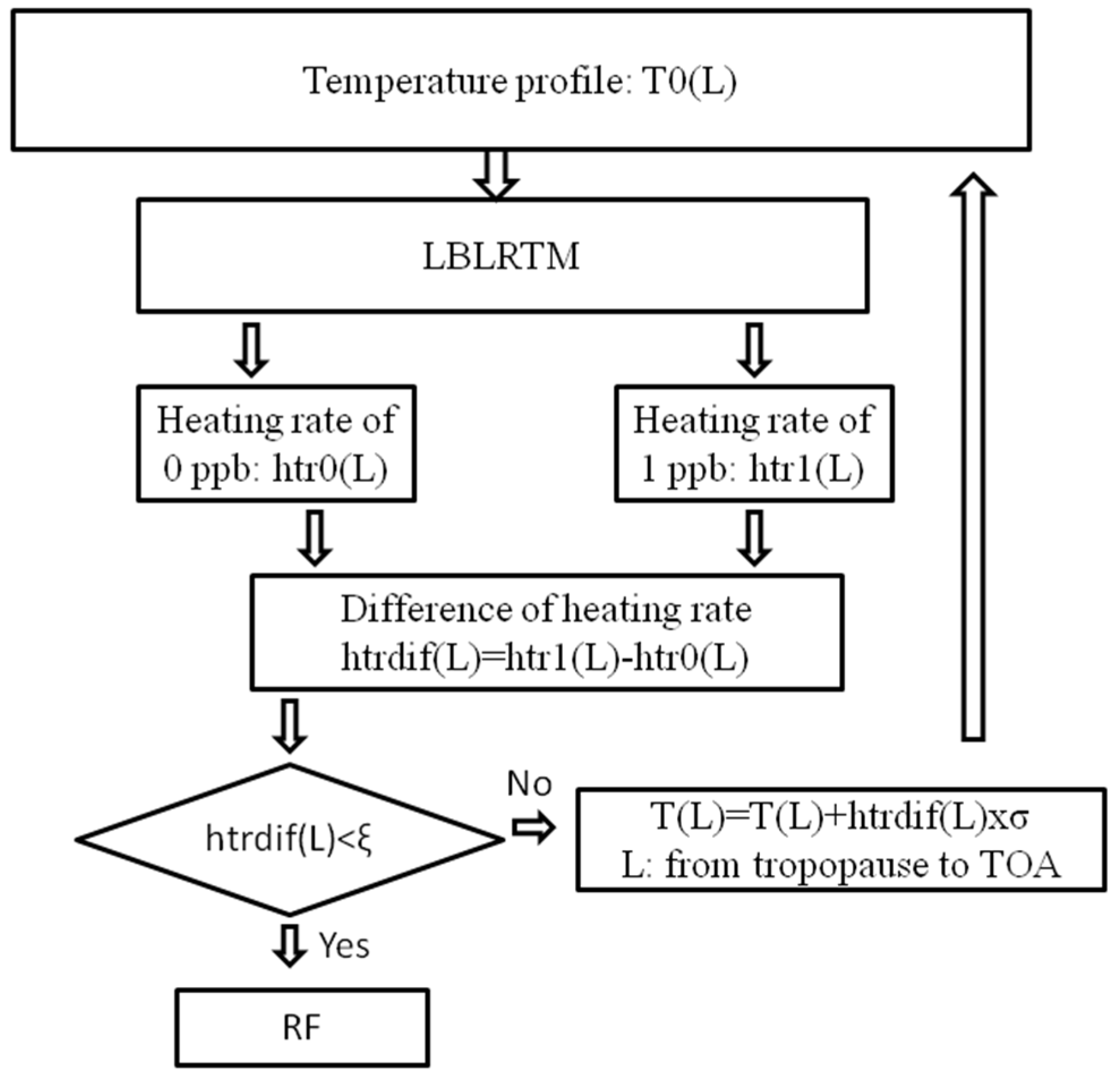
To calculate RF due to NF3, we use an iterative method similar to that presented by Zhang et al. [33,34,35]. Figure 3 provides further information on the iterative method.
The radiative efficiency of NF3 is given as radiative forcing for a 1 ppb increase from zero in global atmospheric concentrations [2]. In Table 3, the instantaneous radiative efficiency (IRE) and radiative efficiency (RE) are calculated for clear, overcast and all sky conditions. In this work, the IRE for clear sky conditions is recorded as 0.242 W·m−2·ppb−1. This is only approximately 2.42% different from Robson et al.’s results [2], which are also based on a line-by-line radiation code. RE is 0.188 W·m−2·ppb−1, as recorded in this work. RE was recorded as 0.211 W·m−2·ppb−1 [2] when using a narrow-band-model, and RE was recalculated as 0.20 W·m−2·ppb−1 [8] based on methods outlined by Pinnock et al. [9]. The difference between our results and those of Hodnebrog et al. [8], which are used in the IPCC AR5, is 6%. However, the difference between the results in this work and Totterdill et al. [10] is large, for in that paper, new NF3 absorption cross-sections was used. We also calculated the NF3 IRE in clear sky conditions with NF3 absorption cross-section data from Totterdill et al. [10], and the difference between the two absorption cross-section data is 0.0096 W·m−2·ppb−1. It is hard to explain the large difference only from different absorption cross-section data.
To quantify and compare the climate impacts of various emissions, it is necessary to consider both RE and lifetime measures. Global warming potential (GWP) and global temperature potential (GTP) are two well-known emission metrics.
GWP is defined as time-integrated radiative forcing due to a pulse emission of a given component relative to a pulse emission of an equal mass of CO2 (IPCC AR5). Compared to GWP, GTP extends one step further down the cause-effect chain. GTP is defined as the change in global mean surface temperature ata chosen point in time in response to an emission pulse relative to that of CO2 (IPCC AR5). The GTP concept can be extended to examine the impact of sustained changes in emissions. We denote sustained changes in GTP as GTPs. In most scenarios, emissions of greenhouse gases are sustained, so GTPs is also calculated. Further information on the calculations of GWP, GTP, and GTPs are included in IPCC AR5 and Shine et al. [36].
The values are shown in Table 4. Here, a lifetime of 740 years is used in Robson et al. [2], a lifetime of 500 years is used in IPCC AR5 and this work, and a lifetime of 509 years is used in Totterdill et al. [10] Robson et al. [2] used the fraction remaining formula of CO2 included in Shine et al. [36], and others have used the formula provided by Joos et al. [37]. Similar to previous discussion in this paper regarding RE and IRE, the differences among Robson et al. [2], IPCC AR5, and this work are small. However, the difference between Totterdill et al. [10] and this work is large.
4. Variability of the NF3Radiative Forcing
The inhomogeneous radiative forcing of homogeneous greenhouse gases including CO2, CH4, and N2O were studied. The vertical temperature change across the atmospheric column (temperature lapse rate) was found to be the best single predictor for explaining forcing variation. In addition, the masking effects of clouds and water vapor also contribute to forcing inhomogeneity [19]. In this work, considering the main absorption cross-section of NF3 is in the atmospheric window area, the surface temperature and cloud are more important to radiative forcing variation and the main absorption gases of water and ozone in atmosphere window area are also considered. In this way, we can get a simple and fast way to calculate NF3 radiative forcing at the top of any atmospheric profile by using a regression model.
4.1. In Clear Sky Conditions
To study the inhomogeneous NF3 radiative forcing caused by atmospheric and surface variables, an ensemble of 42 atmospheric profiles was used [38]. Surface temperature, integrated water content, integrated ozone content, and mean atmospheric temperature of 42 profiles are shown in Table 5. Different atmospheric profiles have different tropopause heights. To avoid the uncertainty from different tropopause heights, we calculate the radiative forcing at the top of the atmosphere.
Table 6 gives the NF3 instantaneous radiative forcing at the top of the atmosphere in clear sky conditions (Fc) in 42 atmospheric profiles with the concentration of 1.0 ppb. From Table 6, Fc ranges from 0.07 W·m−2 to 0.50 W·m−2. The mean value is 0.25 W·m−2.
Surface temperature and Fc have a high positive correlation. The correlation coefficient is 0.94. If surface temperature is used as a single predictor, the determination coefficient R2 is 88%. This means surface temperature can explain 88% of the variation in Fc.
The correlation coefficient between integrated water content and Fc is 0.54, which is not consistent with our knowledge. Considering the overlap absorption between the NF3 and H2O continuum, integrated water content and Fc should be negatively correlated. We find the correlation coefficient between surface temperature and integrated water content to be 0.78. It can be explained in the following way: the correlation coefficient between surface temperature and mean atmospheric temperature is 0.97. When surface temperature is higher, the mean atmospheric temperature is higher, and the high temperature causes the high water vapour content. Thus, in the real atmospheric profile, surface temperature and integrated water content have high positive correlation. To take away the effect of surface temperature, we use partial correlation, which is a method to describe the relationship between two variables while taking away the effects of another variable. The partial correlation coefficient can be calculated by Formula (1)
Here rab_c is the partial correlation coefficient between a and b with the controlling variable c. rab, rac, and rbc are correlation coefficients.
The partial correlation has a high negative correlation coefficient of −0.88 between integrated water content and Fc. This result is both consistent with our knowledge and reasonable.
The correlation coefficient between integrated ozone amount and Fc is −0.54. We also find that the correlation coefficient between surface temperature and integrated ozone amount has a negative correlation coefficient of −0.64. This can be explained in two ways. First, the integrated O3 amount is higher in middle and high latitudes than in low latitudes, and is also higher in cold months than in warm months due to poleward stratospheric air transport. Second, when the integrated ozone amount is larger, it can absorb more solar radiation and thereby reduce the downward radiative flux at the surface. Surface temperature is considered above, by taking away the effect of surface temperature, the partial correlation coefficient between integrated ozone and Fc is 0.20. Since the partial correlation coefficient is small, we not consider integrated ozone in the regression formula.
Based on the consideration above, there is a positive correlation coefficient of 0.94 between Fc and surface temperature. Additionally, there is a negative correlation coefficient of −0.88 between Fc and integrated water content, taking away the effect of surface temperature. Huang et al. [37] used a regression model to study the inhomogeneous radiative forcing of CO2. We use a similar method to study the inhomogeneous radiative forcing of NF3 in clear sky conditions. A prediction model based on the regression method can be calculated by formula (2).
Here Fc0 is the average value of Fc, Ts0 is the average value of Ts, IWC0 is the average value of IWC, and a1 and a2 are coefficients calculated using least-squares method.
The parameters in formula (2) are calculated, according to the least-squares method. Fc0 is 0.25, Ts0 is 279.3, IWC0 is 19.8, a1 is 0.0065, and a2 is 0.0025.
Table 7 shows the differences between Fc calculated using the prediction equation and using the LBLRTM model. The largest relative error is 29.97% based on LBLRTM result, and there are 34 cases in which the relative error is less than 10% based on LBLRTM results. We find that when the relative error is larger, the corresponding absolute error is smaller. The absolute errors of all 42 cases are smaller than 0.044 W·m−2 based on LBLRTM results. The average value of relative error is 6.17% based on LBLRTM results, and the average value of absolute error is 0.013 W·m−2 based on LBLRTM results.
4.2. In Cloudy Sky Conditions
As we all know, clouds can rapidly vary with time and space. As the 42 atmospheric profiles do not provide the cloud profiles, we use USS profile (USA standard) [31] as an example to study the relationship between cloud and NF3 IRF at the top of the atmosphere.
In Table 8, NF3 IRF at the top of the atmosphere in cloudy sky conditions (Fa) with different optical thicknesses and different cloud top pressures are shown. Optical thickness and Fa have a very high negative correlation coefficient of −0.995 when the optical thickness is between 0.39 and 0.73. Cloud top pressure and Fa have a very high positive correlation coefficient of 0.999 when the cloud top pressure is between 436.95 hPa and 702.73 hPa. These correlations suggest that when the optical thickness is small and the cloud top is low, the upward radiative flux at the top of the atmosphere is large and that the large upward radiative flux at the top of the atmosphere can cause large NF3 radiative forcing at the top of the atmosphere.
To establish the relationship between Fc and Fa, the cloud radiative forcing at the top of the atmosphere (CRF) is calculated. CRF and (Fc − Fa) also have a high positive correlation coefficient of 0.985. The prediction equation for Fa is
Here CRF0 is average value of CRF, a3 is coefficient calculated using least-squares method.
According to the least-squares method, a3 is calculated as 0.0049 using the data from Table 8. The average relative error is 5.9% based on LBLRTM results, and the average value of absolute error is 0.01 W·m−2 based on LBLRTM results.
5. Conclusions
In this study, we used a line-by-line method to calculate the global radiative forcing of NF3. In this way, the uncertainty from the overlap absorption between NF3 and other gases can be minimized. In this work, RE was 0.188 W·m−2·ppb−1. The difference between our results and those of Hodnebrog et al. [8], which are used in the IPCC AR5, was 6%. Using the global mean NF3 concentration as 1.24 ppt, the NF3 radiative forcing was 2.33 × 10⁻⁴ W·m−2 which is only about 0.015% that of CO2. Even though NF3 concentrations are growing rapidly, at the moment, their contribution is very small.
The NF3 absorption cross-section is mainly in 800–1100 cm−1. In this region, the main gas absorptions are the H2O continuum absorption and the O3 absorption. To study the inhomogeneity of NF3radiative forcing, 42 atmospheric profiles were used. The instantaneous radiative efficiency was observed to change from 0.07 W·m−2·ppb−1 to 0.50 W·m−2·ppb−1, with a mean value of 0.25 W·m−2·ppb−1.
Surface temperature and Fc displayed a high positive correlation coefficient of 0.94. To remove the effect of surface temperature, partial correlation was used. The partial correlation between integrated water content and Fc was observed to be −0.88 and the partial correlation between integrated ozone and Fc was observed to be 0.20. A regression model was constructed to predict Fc using surface temperature and integrated water content. The average observed value of relative error was 6.17% based on LBLRTM results, and the average observed value of absolute error was 0.013 W·m−2 based on LBLRTM results.
The USS atmospheric profile is an example with which to study the relationship between cloud and NF3 IRF at the top of the atmosphere given different cloud optical depths and different cloud top pressures. CRF and (Fc − Fa) were observed to have a high positive correlation of 0.985. A regression model was constructed to predict Fa using CRF. The average relative error was observed to be 5.9% based on LBLRTM results, and the average value of absolute error was0.01 W·m−2 based on LBLRTM results.
Acknowledgments
The work is supported by the National Natural Science Foundation of China (Grant No. 41305132), the National Natural Science Foundation of China (Grant No. 41575002) and the National Natural Science Foundation of China (Grant No. 91644211).
Author Contributions
The work presented here was carried out in collaboration with all authors. Peng Lu designed, performed the calculation and wrote the manuscript; Hua Zhang and Jinxiu Wu contributed to the reviewing and revising of the manuscript.
Conflicts of Interest
The authors declare no conflict of interest.
References
- Arnold, T.; Harth, C.M.; Muhle, J.; Manning, A.J.; Salameh, P.K.; Kim, J.; Ivy, D.J.; Steele, L.P.; Petrenko, V.V.; Severinghaus, J.P.; et al. Nitrogen trifluoride global emissions estimated from updated atmospheric measurements. Proc. Natl. Acad. Sci. USA 2013, 110, 2029–2034. [Google Scholar] [CrossRef] [PubMed]
- Robson, J.; Gohar, L.; Hurley, M.; Shine, K.; Wallington, T. Revised IR spectrum, radiative efficiency and global warming potential of nitrogen trifluoride. Geophys. Res. Lett. 2006, 33, 10817. [Google Scholar] [CrossRef]
- Myhre, G.; Shindell, D.; Bréon, F.M.; Collins, W.; Fuglestvedt, J.; Huang, J.; Koch, D.; Lamarque, J.F.; Lee, D.; Mendoza, B.; et al. Anthropogenic and Natural Radiative Forcing. In Climate Change 2013: The Physical Science Basis; Contribution of Working Group I to the Fifth Assessment Report of the Intergovernmental Panel on Climate Change; Cambridge University Press: Cambridge, UK, 2013. [Google Scholar]
- Weiss, R.F.; Mühle, J.; Salameh, P.K.; Harth, C.M. Nitrogen trifluoride in the global atmosphere. Geophys. Res. Lett. 2008, 35, 20821. [Google Scholar] [CrossRef]
- Arnold, T.; Mühle, J.; Salameh, P.K.; Harth, C.M.; Ivy, D.J.; Weiss, R.F. Automated measurement of nitrogen trifluoride in ambient air. Anal. Chem. 2012, 84, 4798–4804. [Google Scholar] [CrossRef] [PubMed]
- Houghton, J.; Ding, Y.; Griggs, D.J.; Noguer, M.; van der Linden, P.J.; Dai, X.; Maskell, K.; Johnson, C.A. IPCC 2001: Climate Change 2001, The Climate Change Contribution of Working Group I to the Third Assessment Report of the Intergovemmental Panel on Climate Change 159; IPCC: Geneva, Switzerland, 2001. [Google Scholar]
- Molina, L.T.; Wooldridge, P.J.; Molina, M.J. Atmospheric reactions and ultraviolet and infrared absorptivities of nitrogen trifluoride. Geophys. Res. Lett. 1995, 22, 1873–1876. [Google Scholar] [CrossRef]
- Hodnebrog, Ø.; Etminan, M.; Fuglestvedt, J.; Marston, G.; Myhre, G.; Nielsen, C.; Shine, K.; Wallington, T. Global warming potentials and radiative efficiencies of halocarbons and related compounds: A comprehensive review. Rev. Geophys. 2013, 51, 300–378. [Google Scholar] [CrossRef]
- Pinnock, S.; Hurley, M.D.; Shine, K.P.; Wallington, T.J.; Smyth, T.J. Radiative forcing of climate by hydrochlorofluorocarbons and hydrofluorocarbons. J. Geophys. Res.Atmos. 1995, 100, 23227–23238. [Google Scholar] [CrossRef]
- Totterdill, A.; Kovács, T.; Feng, W.; Dhomse, S.; Smith, C.J.; Gómez–Martín, J.C.; Chipperfield, M.P.; Forster, P.M.; Plane, J.M.C. Atmospheric lifetimes, infrared absorption spectra, radiative forcings and global warming potentials of NF3 and CF3CF2Cl (CFC-115). Atmos. Chem. Phys. 2016, 16, 11451–11463. [Google Scholar] [CrossRef]
- Forster, P.; Ramaswamy, V.; Artaxo, P.; Berntsen, T.; Betts, R.; Fahey, D.W.; Haywood, J.; Lean, J.; Lowe, D.C.; Myhre, G.; et al. Changes in Atmospheric Constituents and in Radiative Forcing; The Physical Science Basis; Intergovernmental Panel on Climate Change: Cambridge, UK, 2007. [Google Scholar]
- Prather, M.J.; Hsu, J. NF3, the greenhouse gas missing from Kyoto. Geophys. Res. Lett. 2008, 35, 12810. [Google Scholar] [CrossRef]
- Sorokin, V.; Gritsan, N.; Chichinin, A. Collisions of O (1D) with HF, F2, XeF2, NF3, and CF4: Deactivation and reaction. J. Chem. Phys. 1998, 108, 8995–9003. [Google Scholar] [CrossRef]
- Olsen, S.; McLinden, C.; Prather, M. Stratospheric N2O–NOy system: Testing uncertainties in a three-dimensional framework. J. Geophys. Res. Atmos. 2001, 106, 28771–28784. [Google Scholar] [CrossRef]
- Wild, O.; Prather, M.J. Global tropospheric ozone modeling: Quantifying errors due to grid resolution. J. Geophys. Res.Atmos. 2006, 111, 11305. [Google Scholar] [CrossRef]
- Dillon, T.J.; Vereecken, L.; Horowitz, A.; Khamaganov, V.; Crowley, J.N.; Lelieveld, J. Removal of the potent greenhouse gas NF3 by reactions with the atmospheric oxidants O (1D), OH and O3. Phys. Chem. Chem. Phys. 2011, 13, 18600–18608. [Google Scholar] [CrossRef] [PubMed]
- World Meteorological Organization (WMO). Scientific Assessment of Ozone Depletion: 2010, Global Ozone Research and Monitoring Project—Report No. 50; World Meteorological Organization: Geneva, Switzerland, 2011; p. 572.
- Papadimitriou, V.C.; McGillen, M.R.; Fleming, E.L.; Jackman, C.H.; Burkholder, J.B. NF3: UV absorption spectrum temperature dependence and the atmospheric and climate forcing implications. Geophys. Res. Lett. 2013, 40, 440–445. [Google Scholar] [CrossRef]
- Huang, Y.; Tan, X.; Xia, Y. Inhomogeneous radiative forcing of homogeneous greenhouse gases. J. Geophys. Res. Atmos. 2016, 121, 2780–2789. [Google Scholar] [CrossRef]
- Clough, S.A.; Iacono, M.J.; Moncet, J.L. Line-by-line calculations of atmospheric fluxes and cooling rates: Application to water vapor. J. Geophys. Res.Atmos. 1992, 97, 15761–15785. [Google Scholar] [CrossRef]
- Clough, S.A.; Shepard, M.W.; Mlawer, E.J.; Delamere, J.S.; Jacono, M.J.; Cady-Pereira, K.; Boukabara, S.; Brown, P.D. Atmospheric radiative transfer modeling: A summary of the AER codes. J. Quant. Spectrosc. Radiat. Transf. 2005, 91, 233–244. [Google Scholar] [CrossRef]
- Delamere, J.; Clough, S.; Payne, V.; Mlawer, E.; Turner, D.; Gamache, R. A far-infrared radiative closure study in the Arctic: Application to water vapor. J. Geophys. Res. Atmos. 2010, 115, 17106. [Google Scholar] [CrossRef]
- Mlawer, E.J.; Payne, V.H.; Moncet, J.L.; Delamere, J.S.; Alvarado, M.J.; Tobin, D.C. Development and recent evaluation of the MT_CKD model of continuum absorption. Philos. Trans. R. Soc. A 2012, 370, 2520–2556. [Google Scholar] [CrossRef] [PubMed]
- Shephard, M.; Clough, S.; Payne, V.; Smith, W.; Kireev, S.; Cady-Pereira, K. Performance of the line-by-line radiative transfer model (LBLRTM) for temperature and species retrievals: IASI case studies from JAIVEx. Atmos. Chem. Phys. 2009, 9, 7397–7417. [Google Scholar] [CrossRef]
- Rothman, L.S.; Gordon, I.E.; Babikov, Y.; Barbe, A.; Chris Benner, D.; Bernath, P.F.; Birk, M.; Bizzocchi, L.; Boudon, V.; Brown, L.R.; et al. The HITRAN2012 molecular spectroscopic database. J. Quant. Spectrosc. Radiat. Transf. 2013, 130, 4–50. [Google Scholar] [CrossRef]
- Rossow, W.B.; Schiffer, R.A. Advances in understanding clouds from ISCCP. Bull. Am. Meteorol. Soc. 1999, 80, 2261–2287. [Google Scholar] [CrossRef]
- Lu, P.; Zhang, H.; Li, J. Correlated k-distribution treatment of cloud optical properties and related radiative impact. J. Atmos. Sci. 2011, 68, 2671–2688. [Google Scholar] [CrossRef]
- Freckleton, R.; Highwood, E.; Shine, K.; Wild, O.; Law, K.; Sanderson, M. Greenhouse gas radiative forcing: Effects of averaging and inhomogeneities in trace gas distribution. Q. J. Roy. Meteor. Soc. 1998, 124, 2099–2127. [Google Scholar] [CrossRef]
- Myhre, G.; Stordal, F. Role of spatial and temporal variations in the computation of radiative forcing and GWP. J. Geophys. Res.Atmos. 1997, 102, 11181–11200. [Google Scholar] [CrossRef]
- Myhre, G.; Stordal, F.; Gausemel, I.; Nielsen, C.J.; Mahieu, E. Line-by-line calculations of thermal infrared radiation representative for global condition: CFC-12 as an example. J. Quant. Spectrosc. Radiat. Transf. 2006, 97, 317–331. [Google Scholar] [CrossRef]
- Anderson, G.P.; Clough, S.A.; Kneizys, F.X.; Chetwood, J.H.; Shettle, E.P. AFGL Atmospheric Constituent Profile (0–120 km); AFGL Technic Report, AFGL-TR-0110; Air Force Geophysics Laboratory: Bedford, MA, USA, 1986. [Google Scholar]
- Kato, S.; Loeb, N.G.; Rose, F.G.; Doelling, D.R.; Rutan, D.A.; Caldwell, T.E.; Yu, L.; Weller, R.A. Surface irradiances consistent with CERES-derived top-of-atmosphere shortwave and longwave irradiances. J. Clim. 2013, 26, 2719–2740. [Google Scholar] [CrossRef]
- Zhang, H.; Wu, J.; Lu, P. A study of the radiative forcing and global warming potentials of hydrofluorocarbons. J. Quant. Spectrosc. Radiat. Transf. 2011, 112, 220–229. [Google Scholar] [CrossRef]
- Zhang, H.; Wu, J.; Shen, Z. Radiative forcing and global warming potential of perfluorocarbons and sulfur hexafluoride. Sci. China D 2011, 54, 764–772. (In Chinese) [Google Scholar] [CrossRef]
- Zhang, H.; Zhang, R.; Shi, G. An updated estimation of radiative forcing due to CO2 and its effect on global surface temperature change. Adv. Atmos. Sci. 2013, 30, 1017–1024. [Google Scholar] [CrossRef]
- Shine, K.P.; Fuglestvedt, J.S.; Hailemariam, K.; Stuber, N. Alternatives to the global warming potential for comparing climate impacts of emissions of greenhouse gases. Clim. Chang. 2005, 68, 281–302. [Google Scholar] [CrossRef]
- Joos, F.; Roth, R.; Fuglestvedt, J.S.; Peters, G.P.; Enting, I.G.; von Bloh, W.; Brovkin, V.; Burke, E.J.; Eby, M.; Edwards, N.R.; et al. Carbon dioxide and climate impulse response functions for the computation of greenhouse gas metrics: A multi-model analysis. Atmos. Chem. Phys. 2013, 13, 2793–2825. [Google Scholar] [CrossRef]
- Garand, L.; Turner, D.S.; Larocque, M.; Bates, J.; Boukabara, S.; Brunel, P.; Chevallier, F.; Deblonde, G.; Engelen, R.; Hollingshead, M.; et al. Radiance and Jacobianintercomparison of radiative transfer models applied to HIRS and AMSU channels. J. Geophys. Res. Atmos. 2001, 106, 24017–24031. [Google Scholar] [CrossRef]
Figure 1.
NF3 absorption cross-section between 400 cm−1 and 2000 cm−1.
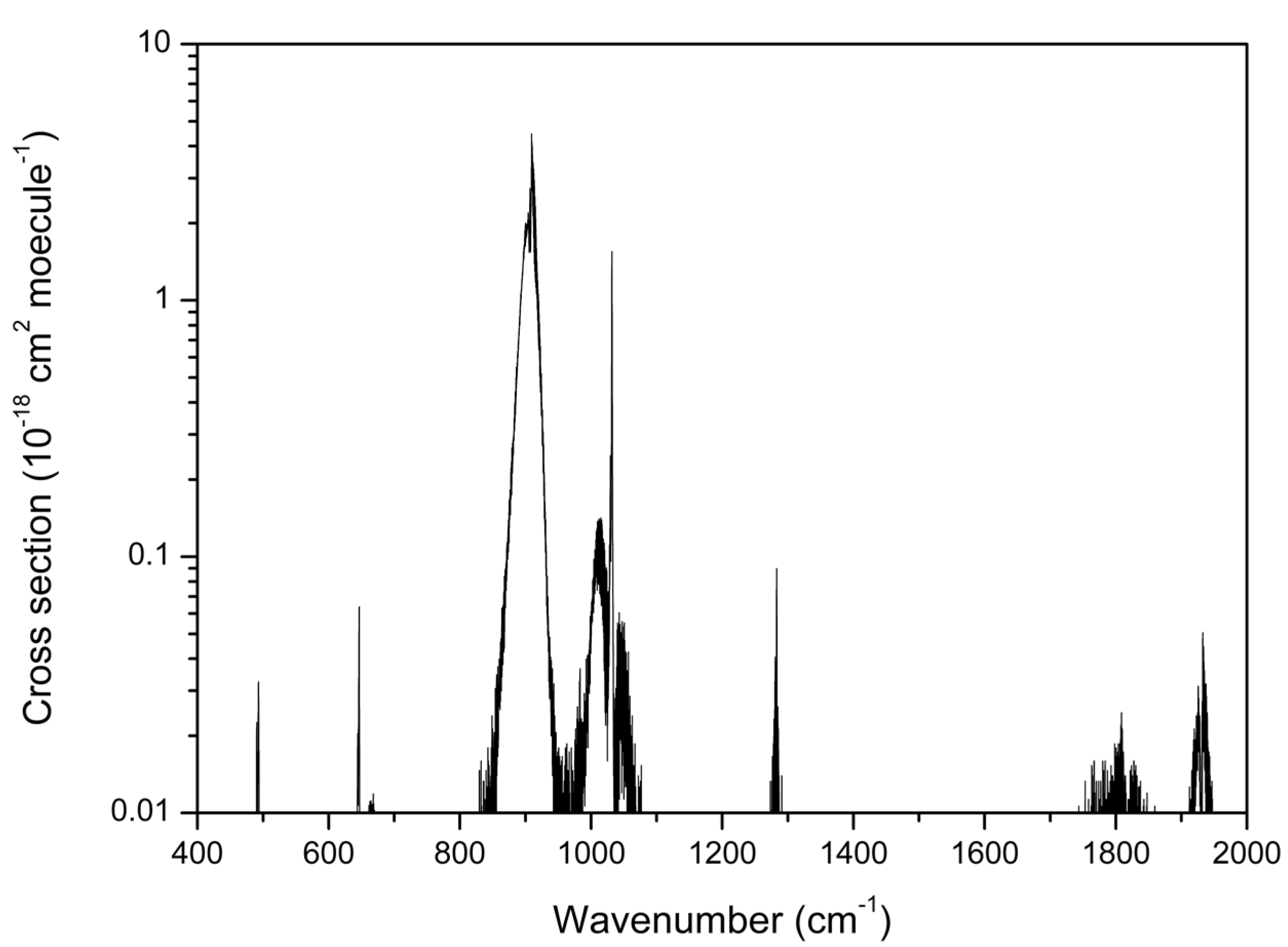
Figure 2.
H2O self and foreign continuum, O3, and NF3 absorption intensity between 800 cm−1 and 1100 cm−1.
Figure 2.
H2O self and foreign continuum, O3, and NF3 absorption intensity between 800 cm−1 and 1100 cm−1.
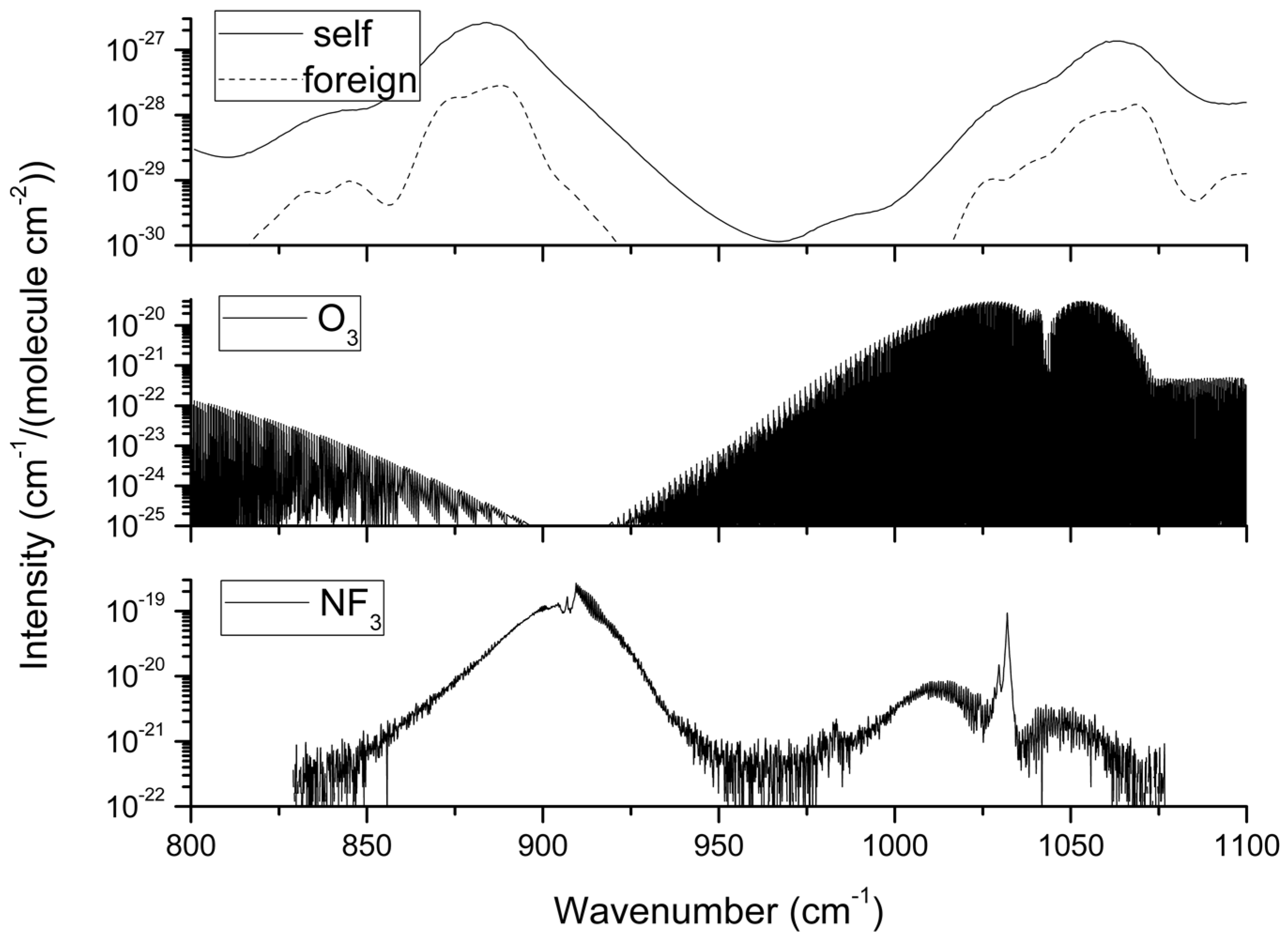
Figure 3.
Schematic of stratospherically adjusted radiative forcing is shown. (L denotes the layer number, T0 is the old temperature profile, T is the new temperature profile, htr0 is the heating rate with no NF3, htr1 is the heating rate with the NF3 of 1 ppb, htrdif is the difference between htr1 and htr0, ξ is the convergence value, and σ is a multiple of htrdif. RF is radiative forcing. Here, the value of σ is 5).

| Level | P (hPa) | Level | P (hPa) | Level | P (hPa) | Level | P (hPa) |
|---|---|---|---|---|---|---|---|
| 1 | 0.10 | 12 | 35.11 | 23 | 253.71 | 34 | 702.73 |
| 2 | 0.29 | 13 | 45.29 | 24 | 286.60 | 35 | 749.12 |
| 3 | 0.69 | 14 | 56.73 | 25 | 321.50 | 36 | 795.09 |
| 4 | 1.42 | 15 | 69.97 | 26 | 358.28 | 37 | 839.95 |
| 5 | 2.61 | 16 | 85.18 | 27 | 396.81 | 38 | 882.80 |
| 6 | 4.41 | 17 | 102.05 | 28 | 436.95 | 39 | 922.46 |
| 7 | 6.95 | 18 | 122.04 | 29 | 478.54 | 40 | 957.44 |
| 8 | 10.37 | 19 | 143.84 | 30 | 521.46 | 41 | 985.88 |
| 9 | 14.81 | 20 | 167.95 | 31 | 565.54 | 42 | 1005.43 |
| 10 | 20.40 | 21 | 194.36 | 32 | 610.60 | 43 | 1013.25 |
| 11 | 27.26 | 22 | 222.94 | 33 | 656.43 |
Table 2.
Global mean radiative flux results from the Line-by-Line Radiative Transfer Model (LBLRTM) using the average of three atmospheric profiles and observations are compared.
| TRO | MLS | MLW | Mean | Observation | ||
|---|---|---|---|---|---|---|
| TOA (Top of Atmosphere) | Clear-sky | 289.8 | 282.7 | 232.2 | 268.2 | 264–266 |
| All-sky | 257.5 | 251.4 | 204.5 | 237.8 | 237–240 | |
| Surface | Down (clear sky) | 394.2 | 349.3 | 224.3 | 322.6 | 314 |
| Up (clear sky) | 457.3 | 424.7 | 311.3 | 397.8 | 397–398 | |
| Down (all sky) | 410.5 | 371.5 | 253.4 | 345.1 | 342–344 | |
| Up (all sky) | 457.3 | 424.7 | 311.3 | 397.8 | 398 |
Table 3.
NF3 instantaneous radiative efficiency (IRE) and radiative efficiency (RE) from the LBLRTM and from other works are compared. TRO, MLS, and MLW refers to tropical, mid-latitude summer, and mid-latitude winter model atmospheric profiles, respectively.
| TRO | MLS | MLW | Mean | References | ||
|---|---|---|---|---|---|---|
| IRE | Clear-sky | 0.296 | 0.260 | 0.170 | 0.242 | 0.248 [2]; 0.35 [10] |
| Overcast-sky | 0.173 | 0.147 | 0.097 | 0.139 | ||
| All-sky | 0.214 | 0.185 | 0.122 | 0.174 | 0.22 [10] | |
| RE | Clear-sky | 0.319 | 0.280 | 0.175 | 0.258 | 0.40 [10] |
| Overcast-sky | 0.194 | 0.163 | 0.102 | 0.153 | ||
| All-sky | 0.236 | 0.202 | 0.127 | 0.188 | 0.211 [2]; 0.20 (IPCC AR5); 0.25 [10] |
Table 4.
A comparison of global warming potential (GWP), global temperature potential (GTP), and sustained changes in GTP (GTPs) results of this work relative to those of other works.
| This Work | References | |
|---|---|---|
| GWP 20 | 11,700 | 12,300 [2], 12,800 (IPCC AR5), 15,600 [10] |
| GWP 100 | 14,700 | 17,200 [2], 16,100 (IPCC AR5), 19,700 [10] |
| GTP 20 | 12,600 | 13,700 (IPCC AR5) |
| GTP 100 | 16,600 | 18,100 (IPCC AR5) |
| GTPs 20 | 10,900 | |
| GTPs 100 | 13,700 |
Table 5.
Atmospheric profile characteristics in terms of surface temperature (Ts), Integrated Water Content (IWC), Integrated Ozone Content (IOC), and Mean Atmospheric Temperature (Tbar).
| Profile | Ts (K) | IWC (kg·m−2) | IOC (DU) | Tbar (K) | Profile | Ts (K) | IWC (kg·m−2) | IOC (DU) | Tbar (K) |
|---|---|---|---|---|---|---|---|---|---|
| 1 | 299.7 | 40.7 | 276.3 | 258.3 | 22 | 314.8 | 19.6 | 268.6 | 264.5 |
| 2 | 294.2 | 29.1 | 330.5 | 258.1 | 23 | 299.5 | 22.01 | 231.1 | 259.9 |
| 3 | 272.1 | 8.3 | 373.7 | 244.6 | 24 | 281.7 | 33.9 | 230.7 | 255.6 |
| 4 | 287.4 | 21.0 | 343.5 | 254.0 | 25 | 292.4 | 37.3 | 270.6 | 255.7 |
| 5 | 257.2 | 4.1 | 371.2 | 237.6 | 26 | 296.9 | 45.0 | 255.8 | 258.2 |
| 6 | 288.2 | 14.1 | 340.2 | 250.4 | 27 | 301.4 | 52.2 | 270.7 | 259.8 |
| 7 | 247.3 | 3.1 | 205.8 | 227.5 | 28 | 301.8 | 59.9 | 255.7 | 260.4 |
| 8 | 242.9 | 0.6 | 484.0 | 232.2 | 29 | 298.4 | 61.5 | 217.9 | 259.2 |
| 9 | 258.1 | 8.3 | 334.2 | 236.8 | 30 | 301.6 | 70.9 | 239.1 | 260.7 |
| 10 | 258.1 | 3.0 | 320.6 | 238.2 | 31 | 250.5 | 1.7 | 222.5 | 232.4 |
| 11 | 275.8 | 7.0 | 355.7 | 242.5 | 32 | 299.4 | 26.6 | 255.2 | 259.9 |
| 12 | 277.7 | 9.7 | 343.7 | 243.1 | 33 | 296.3 | 37.3 | 276.4 | 257.6 |
| 13 | 280.0 | 9.9 | 272.4 | 246.1 | 34 | 283.6 | 12.0 | 286.5 | 247.0 |
| 14 | 284.3 | 15.2 | 364.1 | 251.6 | 35 | 273.3 | 7.7 | 317.0 | 244.9 |
| 15 | 284.7 | 26.0 | 262.7 | 254.0 | 36 | 254.2 | 3.7 | 338.4 | 238.0 |
| 16 | 285.9 | 16.6 | 242.3 | 256.5 | 37 | 261.6 | 5.2 | 371.3 | 241.1 |
| 17 | 302.5 | 51.1 | 235.9 | 259.8 | 38 | 270.7 | 3.8 | 384.3 | 237.0 |
| 18 | 315.9 | 33.1 | 271.3 | 263.9 | 39 | 254.1 | 2.3 | 417.9 | 234.8 |
| 19 | 252.2 | 2.4 | 492.7 | 234.5 | 40 | 249.2 | 0.8 | 449.2 | 236.2 |
| 20 | 290.9 | 10.2 | 235.0 | 258.1 | 41 | 253.3 | 2.0 | 470.8 | 237.0 |
| 21 | 285.1 | 12.9 | 331.1 | 248.7 | 42 | 255.4 | 0.7 | 494.8 | 235.3 |
Table 6.
NF3 instantaneous radiative forcing at the top of the atmosphere in clear sky conditions in 42 atmospheric profiles with the concentration of 1.0 ppb.
| Profile | IRF (W·m−2) | Profile | IRF (W·m−2) | Profile | IRF (W·m−2) | Profile | IRF (W·m−2) |
|---|---|---|---|---|---|---|---|
| 1 | 0.34 | 12 | 0.28 | 23 | 0.38 | 34 | 0.31 |
| 2 | 0.31 | 13 | 0.28 | 24 | 0.21 | 35 | 0.23 |
| 3 | 0.22 | 14 | 0.29 | 25 | 0.28 | 36 | 0.11 |
| 4 | 0.28 | 15 | 0.26 | 26 | 0.29 | 37 | 0.15 |
| 5 | 0.14 | 16 | 0.26 | 27 | 0.34 | 38 | 0.26 |
| 6 | 0.33 | 17 | 0.32 | 28 | 0.28 | 39 | 0.13 |
| 7 | 0.12 | 18 | 0.47 | 29 | 0.26 | 40 | 0.09 |
| 8 | 0.07 | 19 | 0.12 | 30 | 0.29 | 41 | 0.11 |
| 9 | 0.15 | 20 | 0.31 | 31 | 0.12 | 42 | 0.15 |
| 10 | 0.14 | 21 | 0.31 | 32 | 0.36 | ||
| 11 | 0.28 | 22 | 0.50 | 33 | 0.32 |
Table 7.
DifferencesinNF3 instantaneous radiative forcing at the top of the atmosphere based upon comparison of the regression model and LBLRTM model results.
| Profile | Difference (%) | Profile | Difference (%) | Profile | Difference (%) | Profile | Difference (%) |
|---|---|---|---|---|---|---|---|
| 1 | −2.09 | 12 | −6.58 | 23 | −1.03 | 34 | −4.91 |
| 2 | 2.76 | 13 | −0.82 | 24 | 8.30 | 35 | 2.97 |
| 3 | 4.77 | 14 | 3.09 | 25 | 3.30 | 36 | 12.48 |
| 4 | 5.58 | 15 | 2.51 | 26 | 3.93 | 37 | 11.11 |
| 5 | 3.78 | 16 | 17.13 | 27 | −7.12 | 38 | −10.92 |
| 6 | −2.54 | 17 | 1.21 | 28 | 6.74 | 39 | −3.38 |
| 7 | −29.97 | 18 | −2.85 | 29 | 1.89 | 40 | 13.55 |
| 8 | −11.53 | 19 | −3.26 | 30 | −6.64 | 41 | 9.13 |
| 9 | −4.89 | 20 | 13.55 | 31 | −8.97 | 42 | −1.79 |
| 10 | 7.08 | 21 | −2.79 | 32 | 0.10 | ||
| 11 | −5.90 | 22 | −4.53 | 33 | −1.60 |
Table 8.
NF3 instantaneous radiative forcing at the top of the atmosphere with different cloud optical thicknesses and different cloud top pressures with the concentration of 1.0 ppb. CRF, cloud radiative forcing.
| Cloud Optical Thickness | Cloud Top Pressure (hPa) | Fa (W·m−2) | Fc (W·m−2) | CRF (W·m−2) | |
|---|---|---|---|---|---|
| 1 | 0.56 | 565.54 | 0.17 | 0.33 | 30.99 |
| 2 | 0.39 | 565.54 | 0.20 | 0.33 | 24.64 |
| 3 | 0.45 | 565.54 | 0.19 | 0.33 | 27.08 |
| 4 | 0.50 | 565.54 | 0.18 | 0.33 | 28.95 |
| 5 | 0.62 | 565.54 | 0.17 | 0.33 | 32.86 |
| 6 | 0.67 | 565.54 | 0.16 | 0.33 | 34.28 |
| 7 | 0.73 | 565.54 | 0.15 | 0.33 | 35.86 |
| 8 | 0.56 | 436.95 | 0.14 | 0.33 | 44.50 |
| 9 | 0.56 | 478.54 | 0.15 | 0.33 | 39.81 |
| 10 | 0.56 | 521.46 | 0.16 | 0.33 | 35.30 |
| 11 | 0.56 | 610.60 | 0.19 | 0.33 | 26.92 |
| 12 | 0.56 | 656.43 | 0.20 | 0.33 | 23.08 |
| 13 | 0.56 | 702.73 | 0.21 | 0.33 | 19.49 |
© 2017 by the authors; licensee MDPI, Basel, Switzerland. This article is an open access article distributed under the terms and conditions of the Creative Commons Attribution (CC-BY) license (http://creativecommons.org/licenses/by/4.0/).
Share and Cite
MDPI and ACS Style
Lu, P.; Zhang, H.; Wu, J. Inhomogeneous Radiative Forcing of NF3. Atmosphere 2017, 8, 17. https://doi.org/10.3390/atmos8010017
AMA Style
Lu P, Zhang H, Wu J. Inhomogeneous Radiative Forcing of NF3. Atmosphere. 2017; 8(1):17. https://doi.org/10.3390/atmos8010017
Chicago/Turabian StyleLu, Peng, Hua Zhang, and Jinxiu Wu. 2017. "Inhomogeneous Radiative Forcing of NF3" Atmosphere 8, no. 1: 17. https://doi.org/10.3390/atmos8010017
Note that from the first issue of 2016, this journal uses article numbers instead of page numbers. See further details here.