Impact of Grid Nudging Parameters on Dynamical Downscaling during Summer over Mainland China


1
Key Laboratory for Semi-Arid Climate Change of the Ministry of Education, College of Atmospheric Sciences, Lanzhou University, Lanzhou 730000, China
2
Shenyang Atmospheric Environment Research Institute, China Meteorological Administration, Shenyang 110016, China
3
Tianjin Institute of Meteorological Science, Tianjin 300074, China
*
Author to whom correspondence should be addressed.
Atmosphere 2017, 8(10), 184; https://doi.org/10.3390/atmos8100184
Submission received: 18 July 2017
/
Revised: 15 September 2017
/
Accepted: 19 September 2017
/
Published: 25 September 2017
(This article belongs to the Special Issue WRF Simulations at the Mesoscale: From the Microscale to Macroscale)
Abstract
:The grid nudging technique is often used in regional climate dynamical downscaling to make the simulated large-scale fields consistent with the driving fields. In this study, we focused on two specific questions about grid nudging: (1) which nudged variable has a larger impact on the downscaling results; and (2) what is the “optimal” grid nudging strategy for each nudged variable to achieve better downscaling result during summer over the mainland China. To solve these queries, 41 three-month-long simulations for the summer of 2009 and 2010 were performed using the Weather Research and Forecasting model (WRF) to downscale National Centers for Environmental Prediction (NCEP) Final Operational Global Analysis (FNL) data to a 30-km horizontal resolution. The results showed that nudging horizontal wind or temperature had significant influence on the simulation of almost all conventional meteorological elements, while nudging water vapor mainly affected the precipitation, humidity, and 500 hPa temperature. As a whole, the optimal nudging time was one hour or three hours for nudging wind, three hours for nudging temperature, and one hour for nudging water vapor. The optimal nudged level was above the planetary boundary layer for almost every nudged variable. Despite these findings, it should be noted that the optimum nudging scheme varied with simulated regions and layers, and dedicated research for different regions, seasons, and model configuration is advisable.
1. Introduction
Due to low temporal-spatial resolutions, global climate models (GCMs) and reanalysis data often cannot meet the requirements for the analysis of regional scale information [1,2,3,4]. To obtain regional meteorological and climate datasets with a high temporal-spatial resolution, downscaling is usually conducted. Popular downscaling methods include statistical downscaling and dynamical downscaling [5,6,7,8]. The former is based on statistical relationships between large- and fine-scale climate information to obtain regional or local atmospheric structures, while the latter nests a regional fine-grid model to GCMs or reanalysis data. The statistical downscaling needs to have enough observation data to establish a statistical model, and is invalid in regions where large-scale climate elements are not correlated with regional climate elements. On the one hand, the dynamical downscaling process is forced by the large-scale fields, such as GCMs or reanalysis data. On the other hand, it uses regional climate models (RCMs) to add more detailed descriptions of physical processes, topography, and land coverage of a regional scale.
The results of dynamical downscaling are influenced by many factors. These factors may be classified into two categories. The first is the defect of physical processes in RCMs, including cloud microphysical processes, land–atmosphere interaction and cumulus convection process etc. [9]. And the second is the choice of initial conditions, boundary conditions, and simulated domains [2]. Due to the influence of the above-mentioned factors, dynamical downscaling contains errors and uncertainties, which accumulate for the integration of RCMs continuously, and make the results of dynamical downscaling gradually deviate from the driving large-scale field. Newtonian relaxation or nudging is a good method to solve this problem as it can effectively assure the dynamic consistency between the simulated large-scale field and the driving field [2,10,11,12,13].
Developed initially for data assimilation, nudging techniques are being increasingly used in regional climate dynamical downscaling. The concrete method is to increase external forcing in one or a few prediction equations in a period before the start of prediction, which makes the model solution approximate to the observation data and realizes dynamic coordination among variables to raise the prediction effect of the model and achieve the purpose of assimilation. The Weather Research and Forecasting (WRF) model is a new-generation meso-scale numerical prediction system jointly developed by the National Center for Atmospheric Research (NCAR), the National Centers for Environmental Prediction (NCEP) in the United States, etc. In recent years, it has been widely used as a regional climate model to achieve downscaling analysis [10,14,15]. Currently, the nudging assimilation methods of the WRF model applied in the dynamical downscaling process mainly include grid nudging [16] and spectral nudging [11]. The parameters affecting grid nudging simulation results mainly include the choice of nudged variables and nudging time, whether nudging is used in all atmosphere layers, etc.
Recently, research on the nudging application and comparison of two nudging schemes (grid nudging and spectral nudging) has been very common [17,18,19,20,21,22,23]; however, a consistent conclusion is still lacking. Logically, spectral nudging is superior to grid nudging [24], but many findings [17,22,23] have shown that, in some cases, grid nudging is better than spectral nudging. However, the two methods nudge different variables: the default nudged variables of grid nudging in WRF are horizontal wind, potential temperature, and water vapor mixing ratio; and spectral nudging nudges geopotential height instead of humidity. To compare these simply is difficult and insufficiently comprehensive. Apart from the different nudged variables, grid nudging is sensitive to nudging time. Spectral nudging is not sensitive to nudging time but sensitive to cut-off wavelength [18]; and the wavelength cannot be set separately for each nudged variable. Considering both of grid nudging and spectral nudging would make it difficult to compare and analyze the role of each nudging parameter. Based on this, the grid nudging was only considered in this study. For grid nudging, it should be first considered that the influence of different nudged variables on the simulated meteorological elements and how to select the nudged variables to achieve a better simulation. Few studies have focused on this issue. Pohl and Crétat et al. [25] explored the impact of nudged variables on the simulation of tropical deep atmospheric convection in the WRF model, and discovered nudging temperature was the most efficient way to reduce bias, that nudging horizontal wind increased the covariance between simulations and daily observations, while the model’s internal variability was drastically reduced and relied heavily on nudged variables and nudging time. Omrani et al. [26] used “Big-Brother experiment” to inspect the influence of nudged variables on regional model downscaling under ideal conditions and discovered nudging tropospheric horizontal wind was the most effective way to improve the simulations of surface temperature, wind, and precipitation. Moreover, nudging tropospheric temperature also had certain positive effect. Nudging tropospheric wind or temperature could directly improve the simulation of geopotential height field, while nudging water vapor improved the simulation of precipitation but did not obviously improve other variables. However, the above-mentioned studies only paid attention to tropical zones, or were based on an ideal test. To consider the impact of nudged variables on dynamical downscaling over the mainland China, further research is needed.
In addition, grid nudging is sensitive to nudging parameters [18]. However, most research [10,21,27] still adopted the default nudging schemes, while only a few studies [10,13,17,18,25,28] have discussed the sensitivity of nudging time and nudged layer. For nudging time, Salameh et al. [13] used a toy model, verified the significant impact of nudging time on regional climate simulation, and predicted the existence of the optimum nudging time that could more effectively resolve small-scale processes not described in GCMs. Bullock et al. [18] applied the nudging method in the WRF model and indicated that an appropriate setting of nudging time could effectively improve the simulation of surface temperature and wind speed. Bowden et al. [17] compared the influence of nudging time on the simulations of meteorological elements and discovered that an increase in nudging time increased variability, but with greater bias. Furthermore, the study put forth the demand for choosing nudging strategy to balance the accuracy and variability of the simulation results. Current researches only stated the change in nudging time will affect simulation results, while few studies discussed which nudging time was more suitable for the simulation of a specific region and variable. For the nudged layer, Lo et al. [10] used WRF with a grid spacing of 36 km over the conterminous U.S. to compare the nudging throughout the whole atmospheric column to the nudging above the planetary boundary layer (PBL) when downscale the NCEP Final Operational Global Analysis (FNL) data. Results indicated the two nudging experiments resulted in much difference in simulated precipitation, nudging above the PBL performed better than nudging all layers. Pohl and Crétat et al. [25] also pointed out that this was less true below the PBL, more turbulent by nature and where the relaxation should be switched off. However, whether there is a more appropriate nudged level or not is still an issue that is yet been discussed. Against this background, this work focuses on selecting an optimum nudging scheme according to practical simulation demand.
Meanwhile, under the background of vast territory and special climate of the mainland China, how to better set nudging parameters to improve the downscaling results of RCMs has become an important issue. Considering the applicability of analysis data varies with area, this may result in variant optimum nudging schemes in different areas, so discussing a set of nudging parameters by area is more appropriate. For the simulated season, the summer is a disaster-prone season, and there are many uncertainties for the research of summer. Thus, the summer is selected to study. In this study, 41 sensitivity experiments with a grid spacing of 30 km over conterminous China were conducted to investigate the performance of grid nudging with different nudging parameters (nudged variables, layers, and nudging time) during summer using one-degree FNL data and the WRF model. It is expected that, by sensitivity analysis to the nudging parameters, reference nudging schemes would be obtained.
This paper is arranged as follows. Section 2 describes grid nudging, the experimental set-up, evaluation data, and methods. Section 3 investigates the sensitivity of the nudged variables, layers, and nudging time, and provides referential nudging schemes. Finally, the discussion and conclusions are presented in Section 4.
2. Data and Methods
2.1. Grid Nudging
This study used the nudging technique introduced by Hoke and Anthest [29], which is based on an empirical 4D data assimilation method. The core approach is to relax the model state towards the observation by adding a non-physical term to one or a few prediction equations. This nudging term is proportional to the difference between the prediction and the observation. In WRF, the popular nudging methods used for dynamical downscaling include grid nudging and spectral nudging. For grid nudging, each grid-point is nudged towards a value that is time-interpolated from analyses. Spectral nudging only drives the RCM on selected spatial scales, and allows model small scales to evolve with no nudging.
In our work, the grid nudging method was adopted. As discussed in Stauffer and Seaman [30], this grid nudging technique was implemented through an extra tendency term in the nudged variable’s equations, e.g.,
is the flux form of variable , where ; is the surface pressure; and is the constant pressure at the top of the model. represents the physical forcing terms, where x is the independent spatial variable and t is time. is a timescale controlling the nudging strength applied to variable (, is the nudging timescale, unit: s). Furthermore, specifies the horizontal, vertical, and time weighting, where . The analysis quality factor, , which ranges between 0 and 1, is based on the quality and distribution of the data used to produce the gridded analysis. denotes the observation analyzed to the grid and interpolated linearly in time to t. In WRF, can be the zonal and meridian wind components (u, v), the potential temperature (θ), or the water vapor mixing ratio (q). Various nudged variables adjust corresponding variables with Equation (1) in each grid-point of WRF. Through the constraint of model internal equations, other meteorological fields are updated simultaneously. Nudging strength, also known as the nudging coefficient, is controlled by the relaxation time, and the smaller the nudging time , the stronger the nudging strength and the closer the RCM analysis field to the observation field . Nudged layers decide which height the nudging technique is applied.
2.2. Experimental Setup
The model used in this study was the 3.6.1 version of the WRF (ARW) model. The simulation was performed over a large domain covering East Asia (Figure 1a) with 260 × 220 horizontal grid points with a 30 km single grid and 28 vertical levels. The model top was at 10 hPa, and the integration time step was set to 150 s. The main physical options included the WRF double moment 6-class microphysical parameterization [31], the CAM longwave and shortwave radiation [32], the unified Noah land surface model [33], the Kain–Fritsch convective parameterization [34], the Yonsei University planetary boundary layer scheme [35], and the Community Land Model version 4.5 lake scheme [36,37]. The experiments used the grid nudging method and assimilated NCEP FNL data with a 6 h interval between analysis times. The relaxation variables included uv, θ, and q. The 1° × 1° FNL data also provided initial and boundary fields for the model. The boundary conditions and sea surface temperature (SST) data were updated every 6 h. The model was integrated from 22 May to 1 September in 2009 and 2010. As per Tang et al. [38] and Lo et al. [10], the initial 10 days were considered as a spin-up period, so only results for 1 June–1 September were used in the analysis. The simulation results in 2010 were used for analysis, and the simulation results in 2009 were used to verify the universality of the referential nudging schemes obtained prior.
From the research of Pohl et al. [25] and Omrani et al. [26], each nudged variable did not have equally important role in the simulated meteorological fields, and even the nudging of some variables did not work or produced a negative effect. Thus, this study basically started with single variable nudged. In this study, a set of 41 simulations was performed for summer 2009 and 2010, including non-nudging experiments (also known as traditional downscaling experiments, or CTL) and nudging experiments with varying single nudged variables (u, v, θ, and q), nudging time (1 h, 3 h, 6 h, 12 h, and 24 h), and nudged levels (above the planetary boundary layer, above 850 hPa, above 700 hPa, and above 500 hPa) as shown in Table 1. Among them, nudging time changed with modification to the nudging coefficient. Nudging times of 1 h, 3 h, 6 h, 12 h, and 18 h were approximately equal to nudging coefficients of 3 × 10⁻⁴, 1 × 10⁻⁴, 5 × 10⁻⁵, 2.5 × 10⁻⁵, and 1.7 × 10⁻⁵, respectively. Nudged level was changed by the adjustment of the model level below which nudging was switched off, and the layers of 850 hPa, 700 hPa, and 500 hPa were approximately equal to the model level of 7, 10, and 13, respectively. Groups 1 and 2 were performed for summer 2009 and 2010, and Group 3 was performed for summer 2010. Following Lo et al. [10], nudging of all layers was not considered and nudging above the PBL was treated as the default nudged layer.
First, the influence of nudged variables on simulation of meteorological elements near the surface (precipitation, 2 m temperature, 2 m relative humidity, and 10 m wind speed) and at 500 hPa (temperature, wind speed, geopotential height, and relative humidity) was analyzed, under the conditions that nudging time was 1 h and nudged levels were above the PBL. Next, different nudging time and nudged levels were performed to discuss the sensitivity to nudging settings for simulated meteorological elements near the surface and at sounding standard layers (1000, 925, 850, 700, 500, 400, 300, 250, 200, 150, and 100 hPa).
2.3. Evaluation Data and Methods
To evaluate the impact of nudged variables, the difference of simulated meteorological elements between nudging experiments and CTL was compared here. Considering that different circulation, climate, and terrain characteristics and the inconsistent applicability of the analysis data in different regions may affect nudging performance, the mainland China was divided into eight sub-regions (as per the regional division of Zhao et al. [39]) to obtain more representative regional results, as shown in Figure 1a. A–H stand for Northeast China, North China, East China, South China, East of Northwest China, West of Northwest China, Southwest China, and Tibet, respectively. Figure 1b shows the topography over the mainland China.
For observation data, there were no available grid data except precipitation. Comparing the Precipitation Grid Data Set of China Automatic Station and CMORPH (provided by China Meteorological Data Service Center website) with station data, the results were very close. Therefore, the daily mean meteorological observation data of 838 ground observation stations and the twice daily standard layers detection data of 129 sounding observation stations from the mainland China (provided by China Meteorological Data Service Center website) were used to evaluate the effects of different nudging time and nudged levels. The number of ground stations available for A–H was 124, 111, 132, 105, 78, 67, 187, and 34, respectively. The number of sounding stations for each area was 21, 11, 13, 13, 18, 17, 28, and 8. The location of observation stations is shown in Figure 1c,d. The main evaluation methods were to interpolate simulation results onto the observation stations, and to quantify the ability of the model to simulate meteorological fields by using root mean square error (RMSE), mean error (ME), and correlation coefficient (CC). Considering the comparison of the overall simulations of different meteorological elements, the mean improvement rate (RATE) based on RMSE is defined here. The definitions of relevant statistical variables are as follows:
where N is the time sample size; is the regional mean of the simulations at time point ; is the regional mean of the observations at time point ; are time means of and , respectively; nx is the number of variables; is the RMSE of CTL; and is the RMSE of the nudging experiment.
The RATE, which was a dimensionless amount, could be used to evaluate multivariable simulation results. The calculation of RATE for simulated meteorological elements near the surface was based on precipitation, 2 m temperature, 2 m relative humidity, and 10 m wind speed. The calculation of RATE for meteorological elements at sounding standard layers was based on geopotential height, temperature, relative humidity, and wind speed. A positive RATE meant that the nudging experiment outperformed CTL, and a larger value indicated more significant improvement, and a negative one suggested CTL was better.
For ME, it is noteworthy that positive and negative bias may offset each other during the calculation and cannot accurately reflect simulations. Therefore, ME only indicated whether the simulation over- or under-estimated the mean magnitude of the observations and could not be used as a standard to measure the nudging scheme was good or bad in this study.
To ensure the reliability of the simulated results, a significance t test of CC was conducted, based on the CC of the samples to estimate whether the parents were correlated. The method was to compare the CC and the threshold of CC which is defined as When CC ≥ , CC passed the t test. The equation to calculate is as follows:
where n is the sample size; and is the statistics t threshold under significance level , which can be obtained from t-tables.
Next, to investigate the universality of the optimal nudging strategy in summer 2010, the RATE of the simulations with the same nudging time schemes in summer 2009 were adopted. In this evaluation, difference and statistical variables were calculated by area.
3. Results
3.1. Sensitivity Analysis to Nudged Variables
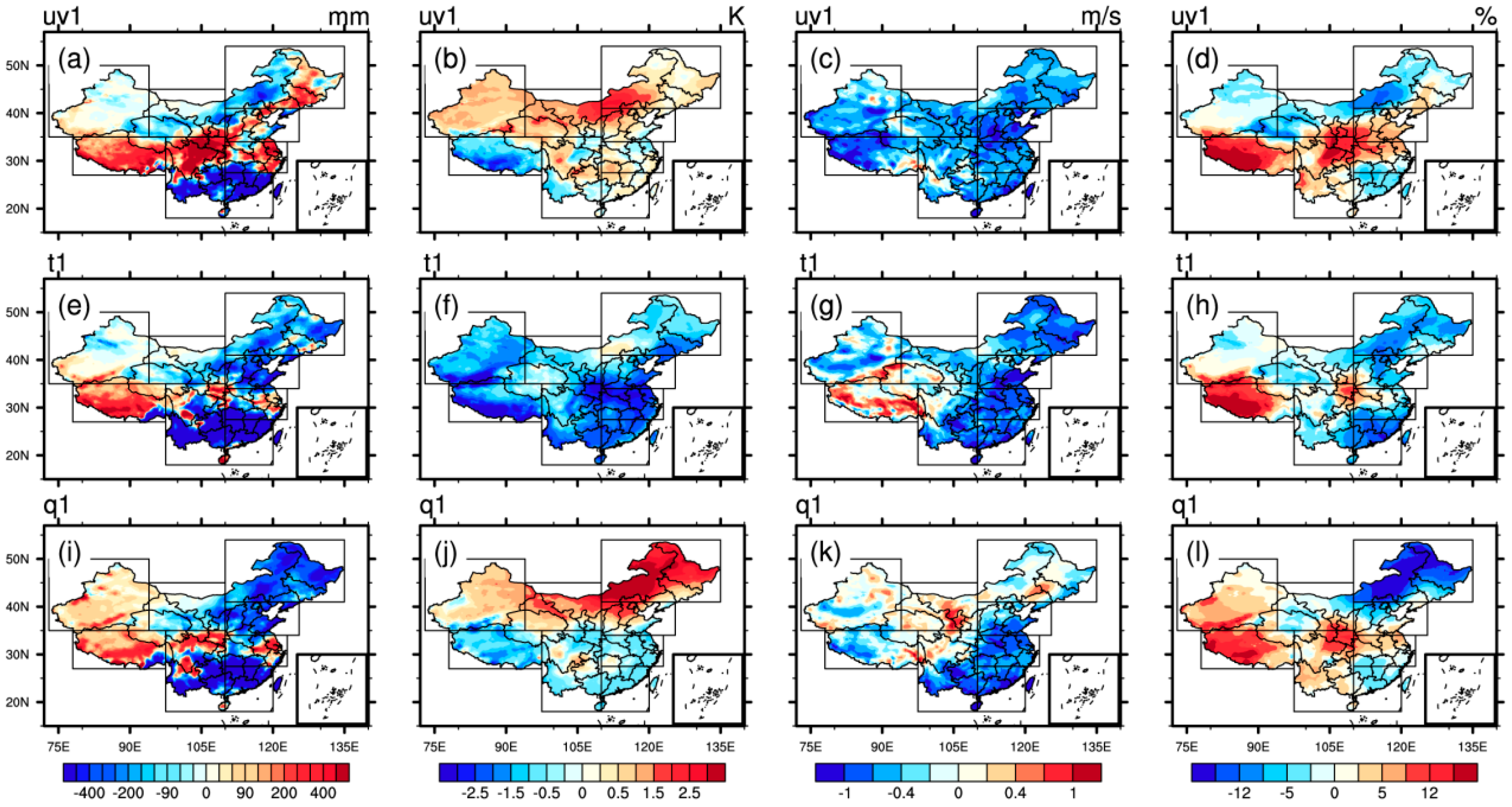
To reveal the impact of different nudged variables on the simulation of meteorological elements, the difference of simulated meteorological elements between the nudging experiments and CTL was compared. The difference field of simulated meteorological elements near the surface (seasonal accumulated precipitation, seasonal mean surface temperature, seasonal mean surface wind speed, and seasonal mean relative humidity) over the mainland China in summer 2010 is shown in Figure 2. Nudging tropospheric uv, θ, or q all had a large influence on the simulation of precipitation. The simulated precipitation was reduced with nudging θ or q in most areas (Figure 2a,e,i). In particular, nudging q had a significant impact on the simulation of precipitation in Northeast (A), and, when uv, θ, or q was nudged, the simulated precipitation increased in Tibet (H) and decreased in South China (D). For the simulation of surface temperature (Figure 2b,f,j), nudging θ had the most significant influence and resulted in the decrease of simulated temperature over almost the whole domain, particularly in East China (C). Nudging uv or q had a weak impact over the mainland China, with the exception of nudging q in Northeast (A). For the simulation of 10 m wind speed (Figure 2c,g,k), nudging tropospheric uv had the strongest influence and decreased simulated wind speed over the entire domain. The impact of nudging θ was also obvious, and nudging q only notably affected North China (B), East China (C), and South China (D). For the 2 m relative humidity simulation (Figure 2d,h,l), the simulations increased obviously in Tibet (H) when uv, θ, or q was nudged. In addition, nudging q in Northeast (A) and nudging uv in Southwest (G) also had an apparent impact on the simulations.
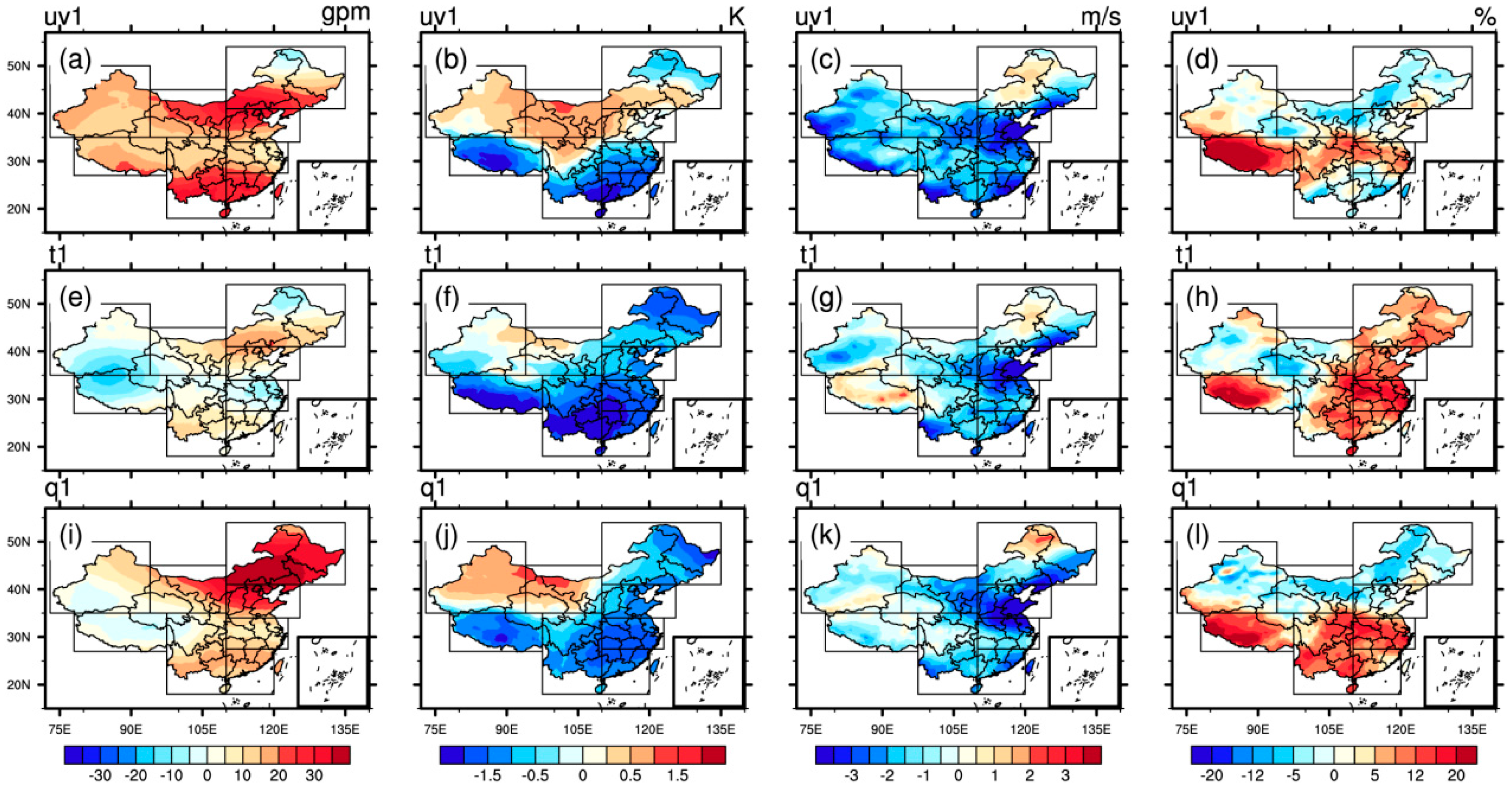
Figure 3 displays the difference field maps of simulated seasonal mean geopotential height, temperature, wind speed, and relative humidity at 500 hPa between the nudging experiments and CTL. From Figure 3a,e,i, it was found that for the simulation of geopotential height at 500 hPa, nudging uv had the strongest influence and resulted in the increase of simulated geopotential height throughout the country; whereas nudging q had a sizable impact in Northeast (A) and North China (B); and nudging θ had a small impact. Similar to the 2 m temperature, nudging tropospheric θ had the most obvious influence on simulations of 500 hPa temperature, where nudging uv or q also had significant influence (Figure 3b,f,j). From Figure 3c,g,k, it was seen that the assimilation of uv had an obvious impact on the simulation of 500 hPa wind speed, and the assimilation of θ or q only had an apparent influence on simulation in North China (B). For the simulation of wind speed at 500 hPa, in most areas of China, the addition of nudging scheme weakened simulated wind speed at 500 hPa. For the simulation of relative humidity (Figure 3d,h,l), nudging uv increased simulations in Tibet (H); nudging θ mainly affected simulations in Eastern China (A–D); and nudging q had a strong influence in Southern China (C, D, G, and H).
In general, nudging uv, θ, or q affected the simulation of meteorological elements near the surface and at 500 hPa, but the main meteorological elements that were influenced and the intensity were different. Specifically, nudging tropospheric uv affected almost all meteorological elements obviously, except for the negligible influence on the simulation of relative humidity at 500 hPa. Nudging θ also had an obvious influence on the simulation of all meteorological elements except 500 hPa geopotential height and wind. Nudging q had weak influence on almost all variables except precipitation, relative humidity, and 500 hPa temperature. The role of nudging q possessed obvious regional characteristics. For the simulation of precipitation, 2 m temperature, 2 m relative humidity, and geopotential height at 500 hPa, nudging q had a sizable influence in Northeast (A).
3.2. Sensitivity Analysis to the Nudging Time
To further reveal the impact of nudging time on meteorological elements near the surface and at different layers, the simulations performed in the absence of nudging and in the presence of nudging with various relaxation time were compared, then apply statistical variables (RATE, ME, and CC) to quantify the effects by area.
The RATE of simulated near-surface meteorological elements was calculated and is listed in Table 2. Of the three nudged variables, nudging θ greatly improved the simulations everywhere, except in Tibet (H). Between nudging uv and q, nudging uv showed more obvious improvement in Northern China (A, B, E, and F), while nudging q showed slightly greater improvement in Southern China (C, D, and G). Of all the concerned areas, the improvement from nudging to the simulated meteorological elements in East China (C) and South China (D) was obviously greater than those in other areas. Specifically, for nudging uv, the simulations benefited the most in Northeast China (A) and Northwest China (E and F) when nudging time was 3 h. Improvement was even greater in North China (B), East China (C), South China (D), and Southwest China (G) when nudging time was 1 h. Furthermore, CTL was better for simulations in Tibet (H). For nudging θ, near-surface meteorological elements were simulated the best when nudging time was 3 h in all areas except North China (B) and Tibet (H). In North China (B) nudging time of 1 h was better, whereas in Tibet (H) the simulations of nudging experiments were worse than that of CTL. For nudging q, improvement was obviously better when nudging time was 1 h in many areas except Northeast China (A), West of Northwest (F), and Tibet (H), where the performance of CTL was better.
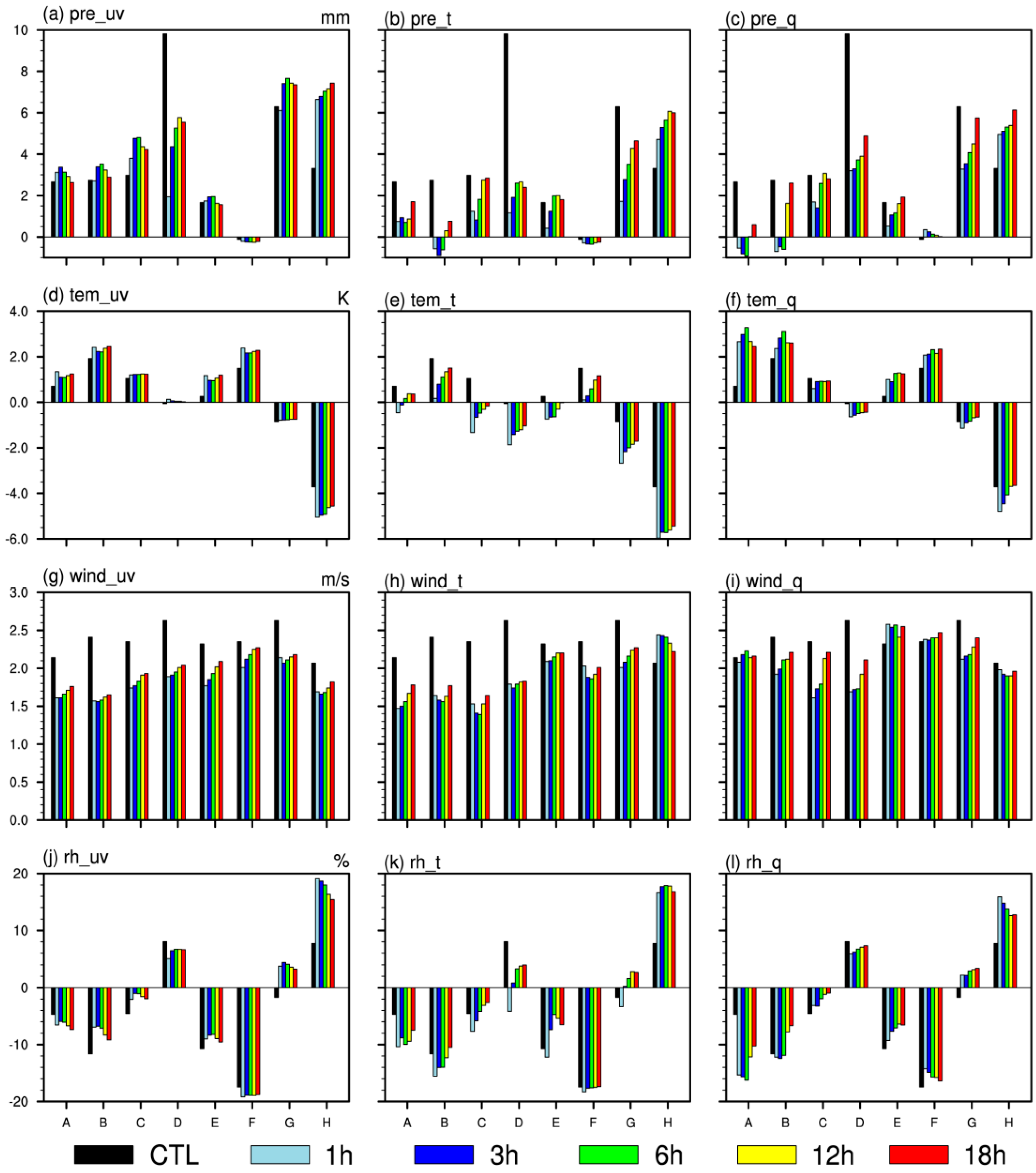
Figure 4 shows the bars for ME of simulated meteorological elements near the surface. For the simulation of precipitation (Figure 4a–c), a wet bias occurred over most areas in all experiments regardless of whether nudging was used. Nudging θ or q adopting higher nudging strength (nudging time 1 h or 3 h) extremely reduced the wet bias of precipitation, particularly in South China (D). Nudging uv did not improve precipitation simulations as perfectly as nudging θ or q except in South China (D). For the simulation of surface temperature (Figure 4d–f), the result simulated from CTL was a cold bias in South China (D), Southwest (G), and Tibet (H) and a warm bias in other areas. Nudging uv or q increased the bias, while nudging θ reduced the warm bias and increased cold bias, particularly in Tibet (H). CTL showed positive bias for the wind speed simulation. The nudging scheme effectively reduced the positive bias of simulated wind speed, and the effect was most significant when nudging time was 1 h or 3 h (Figure 4g–i). In CTL, the relative humidity simulation showed a negative bias in all areas except South China (D) and Tibet (H) (Figure 4j–l). When the nudging scheme was adopted, the simulation of relative humidity in Southwest (G) showed a positive bias conversely.
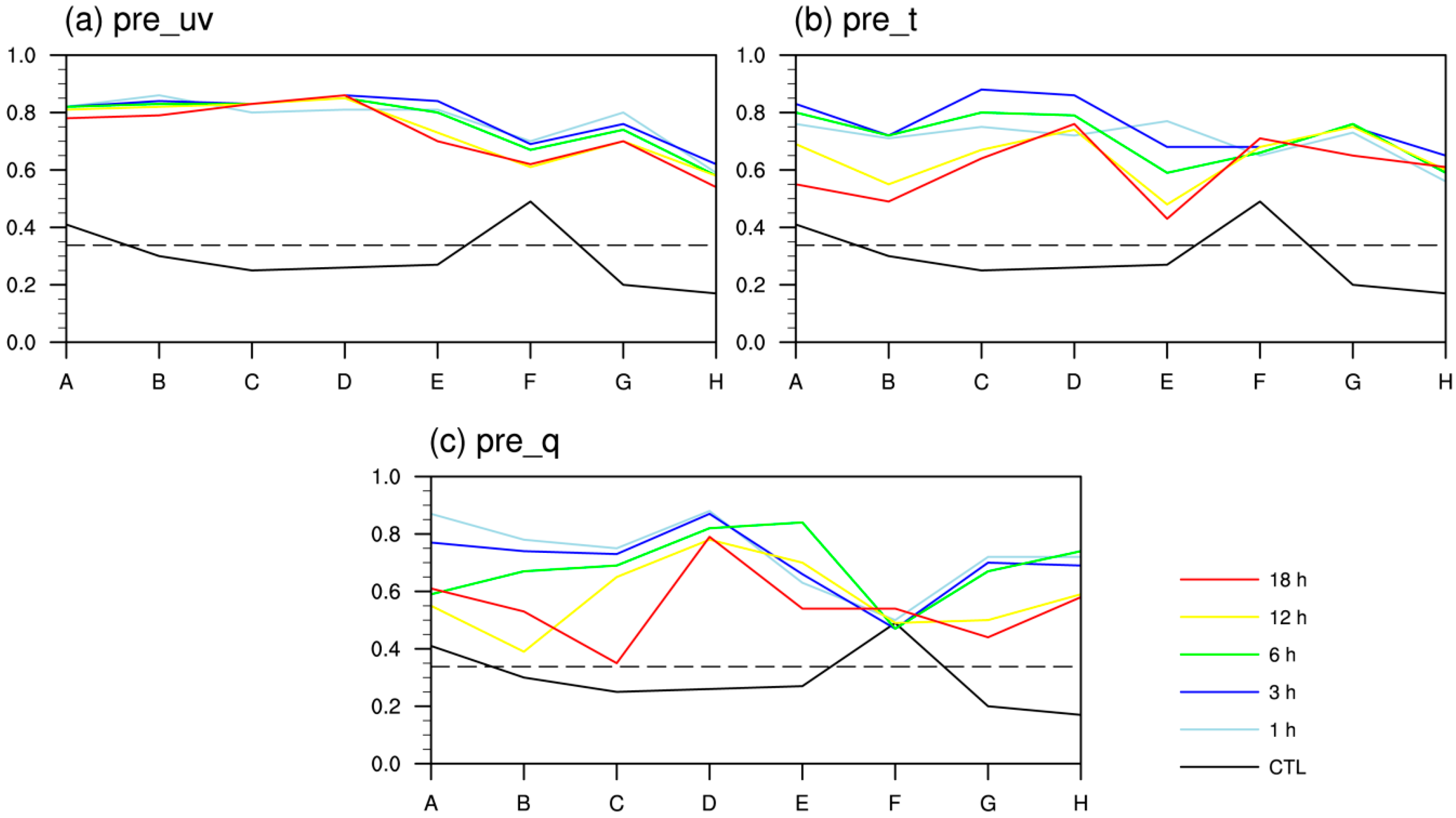
Different schemes were also compared in the correlation of near-surface meteorological elements between simulations and observations. Figure 5 shows the CC about precipitation. For CTL, except in Northeast (A) and West of Northwest (F), the simulated precipitation failed in the significance test at 0.1% significance level. With the presence of nudging, the CC was extremely raised and passed the significance test in each sub-region. A comparison of the different nudging schemes showed that, when uv was nudged, nudging time of 1 h and 3 h had the best performance; when θ was nudged, nudging time of 3 h improved the CC the most except in East of Northwest (E) and Southwest (G); and, when q was nudged, nudging time of 1 h had the best result in almost all areas. It was noted that the CC was slightly poorer in West of Northwest (F) and Tibet (H), than that in other sub-regions. The CC of other near-surface meteorological elements showed similar conclusion. Except for the simulated wind speed when q was nudged in North China (B) and East China (C), the simulation results of all other nudging experiments passed the significance test at a 0.1% significance level.
To compare the overall simulation results of meteorological elements at different sounding levels, this study selected geopotential height, temperature, wind speed, and relative humidity at each standard layer above the surface and analyzed the RATE when nudging scheme was adopted, the results of which are shown in Table 3. Overall, when tropospheric θ was nudged, the simulation improved the most, followed by uv and q. For different regions, the nudging scheme showed more improvement in the simulation of meteorological elements in Eastern China (A–D) than that in Western China (E–H). For nudging uv, there was the most dramatic improvement for simulated meteorological elements in all areas except South China (D) when nudging time was 3 h. Furthermore, in South China (D), nudging time of 1 h improved the simulations more. For nudging θ, the advantage was obvious in all areas when nudging time was 3 h. Finally, for nudging q, nudging time of 1 h provided the best performance.
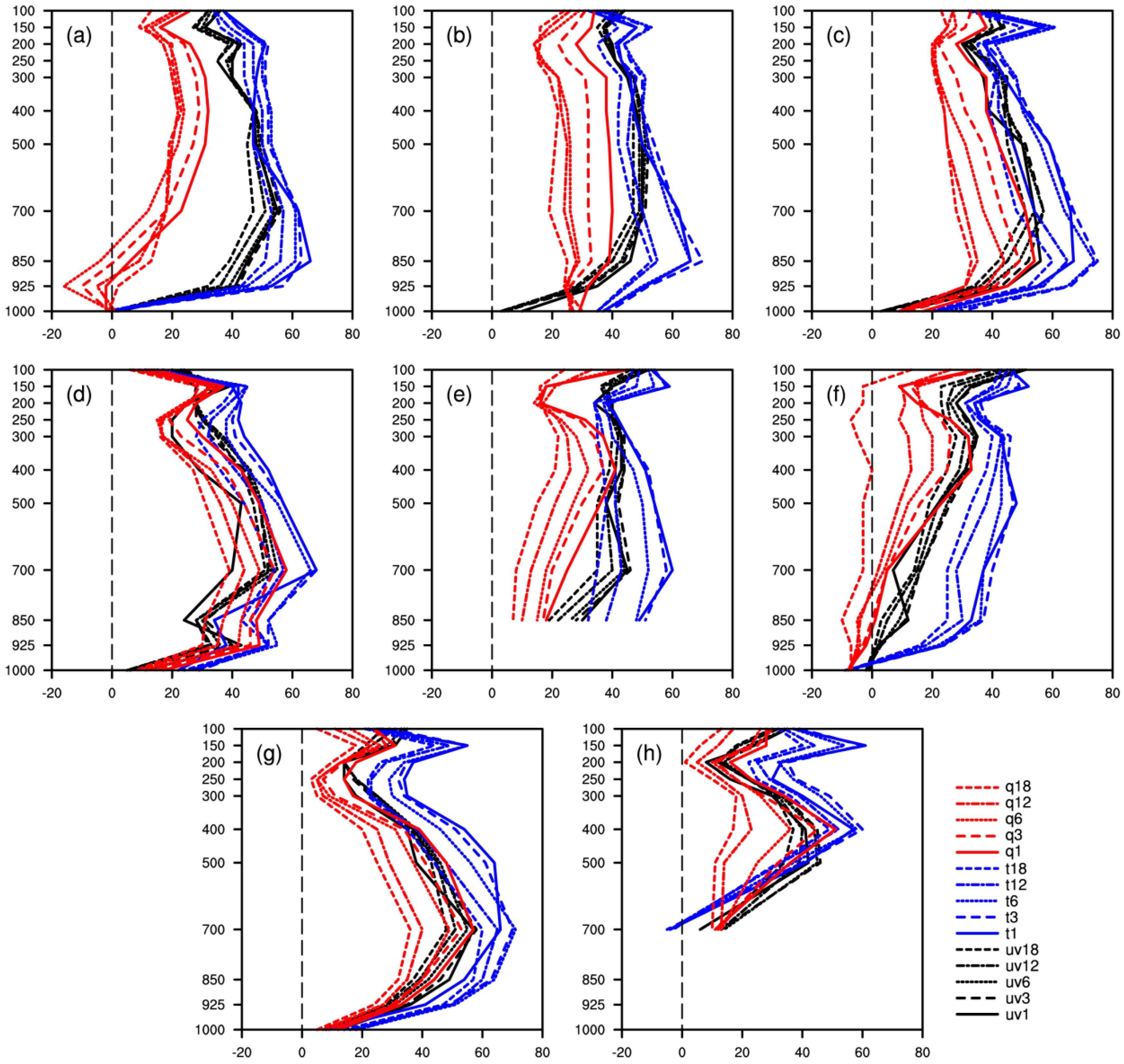
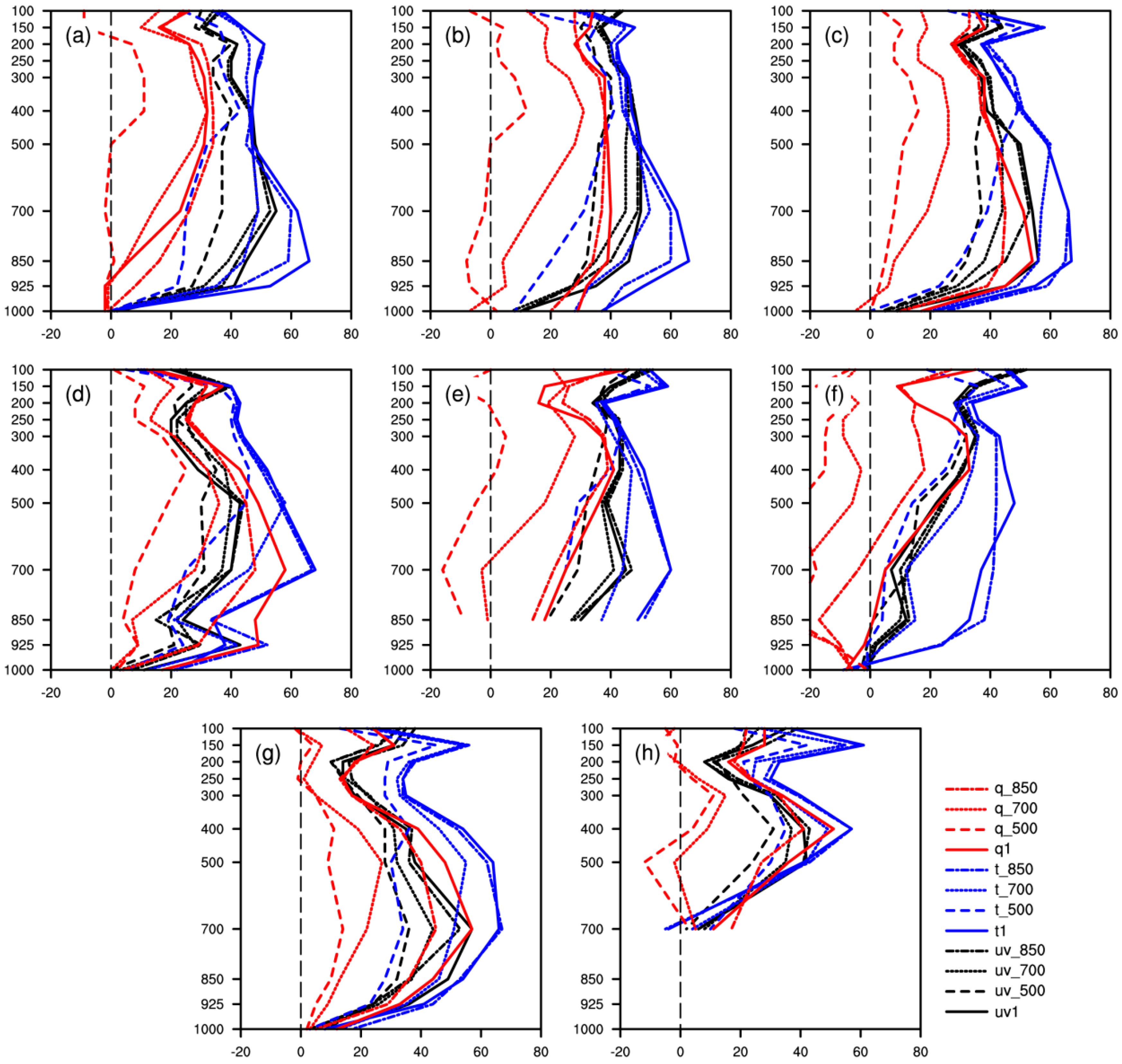
In view of the RATE to simulated meteorological elements in different layers (Figure 6), the layers showing apparent improvement were mainly at 850–400 hPa. At lower levels, the nudging scheme showed poor improvement, especially in Northeast (A) and West of Northwest (F), where even a negative effect appeared when q was nudged. The layers that were more influenced by the setting of different nudging time were also at 850–400 hPa, and the improvement of meteorological elements simulation at lower and upper layers was less sensitive to the change of nudging time. Like the results in Table 3, when an appropriate nudging time was selected, nudging θ improved the simulation the most, and nudging uv was obviously superior to nudging q in Northeast (A), North China (B), and Northwest (E and F). In addition, nudging q at 18 h nudging time nearly appeared the worst performance in each sub-region, especially in West of Northwest (F), where there was always a negative effect from 1000 hPa to 150 hPa.
The ME of the simulated meteorological elements at standard sounding layers was analyzed (data not shown). For geopotential height, the results simulated from CTL at upper levels had an obvious positive bias, and low levels had negative bias. Nudging could effectively reduce the negative bias of the simulation at lower levels. For temperature, wind speed, and relative humidity, the simulation of CTL had positive bias, which meant that the simulated temperature was warmer, wind larger and humidity wetter than the observations. Furthermore, the nudging experiments, particularly nudging θ, could effectively reduce the positive bias of simulated temperature, and nudging also obviously reduced the bias of simulated wind speed at low layers.
Figure 7 illustrates the CC between the simulation and observation of geopotential height at 500 hPa in each region and scheme. The simulated geopotential height of CTL had a high correction with the observed value except in South China (D), and nudging experiments improved it further. In particular, when uv or θ was nudged, the CC of nudging experiments was close to 1 (Figure 7a,b). When uv was nudged, nudging time of 1 h showed the lowest CC, and it was difficult to distinguish which nudging scheme was best; when θ was nudged, nudging time of 3 h provided the best performance; and, when q was nudged, nudging time of 1 h had the highest CC obviously. Comparing the correlation of other meteorological elements between simulations and observations or at other standard layers (not shown), it was concluded that the adoption of nudging scheme could effectively raise the correlations. Except for the simulation of some meteorological elements at 1000 hPa and 925 hPa, all nudged results passed the significance test at a 0.1% significance level.
Among the three nudged variables, nudging θ improved the simulations the most, followed by nudging uv, and nudging q. Moreover, nudging improved the simulation of meteorological elements in Eastern China (A–D) more than that in Western China (E–H). To set nudging time, the effect was best when uv was nudged with nudging time of 1 h or 3 h, when θ was nudged with nudging time of 3 h, and q was nudged with nudging time of 1 h. If a simulation was conducted in different areas, the most suitable nudging time for each area could be selected according to Table 2 and Table 3. From the correlation perspective, the simulated meteorological elements that failed in the significance test when nudging technique was not adopted, could almost all pass the significance test at a 0.1% significance level with the presence of nudging, suggesting that the nudged results were highly reliable.
3.3. Sensitivity Analysis to the Nudged Levels
By comparing the simulation results of meteorological elements with different nudging time, it is noteworthy that nudging above the PBL obviously improved the simulation of meteorological elements at the upper layers, but was not ideal for simulations near the surface and at lower layers in some areas. Thus, it is further considered if the increase of nudged levels could improve the simulation results of meteorological elements near the surface and at low levels, without affecting the simulations at upper levels. In this section, with the nudging time set as 1 h, four groups of sensitivity experiment were designed: the nudged level of above the PBL; above 850 hPa; above 700 hPa; and above 500 hPa. Statistical variables including RATE, ME, and CC were used to evaluate the sensitivity of the simulations to nudged levels.
Table 4 shows the RATE of simulated meteorological elements near the surface with different nudged levels. For nudging tropospheric uv, improvement was especially significant in North China (B), East China (C), and South China (D), when the nudged level was above the PBL. In Northeast (A), East of Northwest (E), and Southwest (G), the simulation result was better when the nudged level was above 850 hPa. However, in Tibet (H), nudging uv showed an adverse effect, and in West of Northwest (F), nudging uv had barely any improvement on near-surface meteorological elements simulations. For nudging θ, except that nudging above the PBL in North China (B), above 700 hPa in South China (D) and Southwest (G) and non-adoption of nudging scheme in Tibet (H) showed a better effect, the improvement was most obvious when the nudged level was above 850 hPa in other areas. For nudging q, the results were similar to the simulations with different nudging time, and the adoption of nudging schemes were not suitable for the simulations in Northeast (A), West of Northwest (F), and Tibet (H). Furthermore, performance was best when the nudged level was above the PBL in other areas. Moreover, the simulations improved the least when the nudged level was above 500 hPa in almost all nudging experiments. In particular, when q was nudged with levels above 500 hPa, the effect was even poorer than that of CTL in most areas.
The ME of the simulated near-surface meteorological elements with different nudged levels was analyzed (data not shown). In general, when compared with the observations, the simulated amount of precipitation was larger and the simulated wind speed stronger; however, the simulated relative humidity showed a drier feature in all areas except South China (D), Southwest (G), and Tibet (H). Thus, it was clear that the addition of nudging scheme could greatly reduce the positive bias for the simulation of precipitation and wind speed, especially when the nudged level was above the PBL.
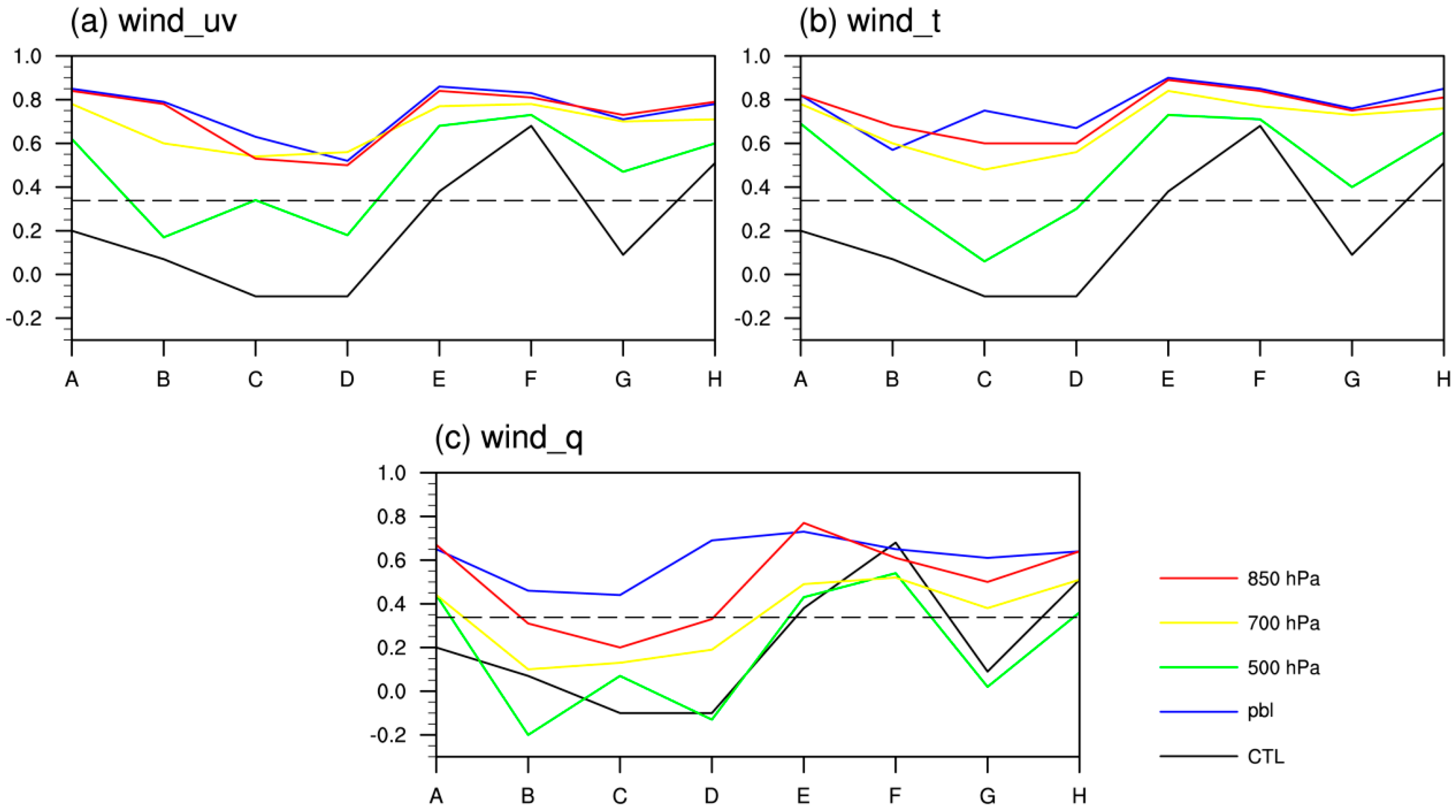
Based on the CC analysis, for the simulation of 2 m wind speed (Figure 8), the CTL provided the lowest CC and failed in the significance t test at 0.1% significance level in all areas except West of Northwest (F) and Tibet (H). When uv or θ was nudged, the CC improved extremely; when q was nudged, the improvement was slight poorer. Among the nudged level schemes, nudging above the PBL provided the best performance, and the performance of nudging above 850 hPa was very close to that of nudging above the PBL. Nudging above 500 hPa was worst, especially when q was nudged as the significant test was not passed in almost all areas. For other near-surface meteorological elements (data not shown), the correlation between the simulations and observations also increased dramatically, when the nudged level was above the PBL or 850 hPa. Furthermore, by the significance t test, the confidence level can reach 99.9%.
To evaluate the simulation results of meteorological elements at vertical layers, the RATE of simulated meteorological elements at standard layers above the surface was calculated and is shown in Table 5. For nudging uv, in Northwest (E and F) and Tibet (H), the simulations had higher skills when the nudged level was above 850 hPa, and, in other areas, improvement was even greater when the nudged level was above the PBL. For nudging θ, the best performance was when the nudged level was above the PBL or 850 hPa. In detail, performance was slightly better when the nudged level was above 850 hPa in East China (C), South China (D), and Southwest (G), and the simulation was best when nudged level was above the PBL in other areas. For nudging q, the simulation was perfect in Northeast (A) when the nudged level was above 850 hPa, and even better in other areas when the level was above the PBL. Consistent with the simulations of near-surface meteorological elements, the overall performance was poorest when the nudged level was above 500 hPa. In particular, nudging q above 500 hPa showed little improvement or even a negative effect on the simulated meteorological elements.
Based on the RATE analysis with varying nudged levels at different layers (shown as Figure 9), in general, nudging θ showed the best behavior, with obvious improvement on the simulation of meteorological elements at 850–400 hPa when the nudged level was above the PBL. Furthermore, the layers that were sensitive to the varying settings of nudged level were also at 850–400 hPa. In addition, when uv or θ was nudged, nudging above 850 hPa or the PBL provided the best performance and showed a small difference. When q was nudged, the RATE varied widely with different nudged level schemes, and nudging above 500 hPa had the poorest improvement out of all nudging schemes. When the nudged level was above 500 hPa, although the overall effect was not ideal, the improvement of simulated meteorological elements above 500 hPa was still obvious.
From the ME analysis for simulated meteorological elements at standard layers with different nudged levels (data not shown), the simulation of geopotential height was higher at the upper levels, and lower at lower levels than the observations. When the nudged level was above the PBL, positive bias was effectively reduced. For temperature, the simulations displayed warm bias as a whole, but nudging θ significantly reduced bias, especially when the nudged level was above the PBL. The simulation of wind speed was also stronger, and nudged simulations had significant improvement at most layers. For relative humidity, when compared with the observation, the simulation was wetter at the upper levels, and drier at low levels. When the nudged level was above the PBL, the negative biases of the simulations at low levels were reduced significantly.
The CC analysis between the simulations and observations of meteorological elements at standard layers (data not shown) revealed that the nudging experiments that adopted different nudged levels significantly improved the correlation between the simulation and observation. In detail, with the exception that the correlation of some meteorological elements at low (1000 hPa and 925 hPa) and upper levels (150 hPa and 100 hPa) could not pass the significance test, the correlation at all other levels passed the significance test at a 0.1% significance level.
The adoption of varying nudged levels showed different effects on simulated meteorological elements near the surface and at standard layers. In general, the optimal nudged level was above the PBL or 850 hPa when uv or θ was nudged and above the PBL when q was nudged. The behavior was poorest in all areas when the nudged level was above 500 hPa. If the simulated domain was divided into different areas, the most suitable nudged levels for different areas could refer to the Table 4 and Table 5. It is noteworthy that for the simulation of meteorological elements near the surface, nudging scheme was not suitable for the simulations in Tibet (H). In addition, in Northeast (A) and West of Northwest (F), the results were better without nudging q. From the perspective of the CC, nudging significantly refined the correlation between the simulation and observation. Meanwhile, almost all simulations of meteorological elements passed the significance test at a 0.1% significance level, suggesting that the simulation results were highly reliable.
3.4. Verification of the Optimum Nudging Scheme
In this section, the universality of the above conclusions was verified. The RATE of the simulated meteorological elements near the surface and at standard layers in summer 2009 with varying nudging time was selected as the key variable to evaluate, and the results are shown in Table 6 and Table 7. For the simulation of near-surface meteorological elements (Table 6), when uv was nudged, the optimum nudging time in 2010 had a very good application, and only in Southwest (G) was the optimum nudging time different. When θ was nudged, nudging time of 3 h still showed the best effect on a whole, but in North China (B), East China (C), South China (D), and Southwest (G), the optimum nudging time was inconsistent with that in 2010. Specifically, when the nudging time in North China (B), East China (C), and Southwest (G) was 6 h and in South China (D) was 12 h, the effect was slightly better. When q was nudged, nudging time of 1 h was still best in most areas, but in Northeast (A), North China (B), and Northwest (E–F), the optimum nudging time was different from that in 2010. Considering the overall simulation of meteorological elements at sounding standard layers (Table 7), as the same with the simulation of meteorological elements near the surface, when uv was nudged the nudging time was also desirably applicable, and the applicability was slightly poor in Tibet (H). When θ or q was nudged, the results obtained in 2010 were fully applicable.
In general, certain universality existed in the referential nudging scheme based on simulated meteorological elements near the surface and at different vertical levels in the summer of 2010. Still, the simulations improved the most when nudging time was 1 h or 3 h for nudging uv, 3 h for nudging θ and 1 h for nudging q, but nudging schemes were variously applicable for different nudged variables, simulated areas and layers. Among the nudged variables, nudging strategy was universally applicable when uv was nudged. Among the concerned areas, the applicability of nudging scheme was better for the simulations in Northeast (A), East China (C), South China (D), East of Northwest (E), and Tibet (H). Between the surface and sounding standard layers, the scheme for the simulation of meteorological elements at sounding layers possessed better applicability.
4. Discussion and Conclusions
The grid nudging technique has been used extensively to prevent dynamical downscaling results from drifting away from the large-scale driving fields. However, the impact of nudging options (nudged variables, layers, and nudging time) and the choice of optimal nudging strategy over the mainland China remains scarce. In this paper, the performances of simulations with varying nudged variables, levels, and nudging time were compared. Using the WRF model as a RCM, 41 continuous sensitivity experiments with different nudging parameters from June to August 2009 and 2010 were evaluated when downscale the FNL data to a 30 km resolution over the mainland China. To compare the impact of nudged variables, this study applied the difference field analysis between the simulations in the absence of nudging and presence of nudging. Furthermore, RATE, ME, and CC were applied to quantify the effect of different nudged layers and nudging time.
Nudging tropospheric horizontal wind, temperature, or water vapor mixing ratio all influenced the simulation of meteorological elements near the surface and at 500 hPa. Of the three nudged variables, nudging tropospheric uv affected more variables. Except for a weak impact on the simulation of 500 hPa relative humidity, nudging uv significantly affected the simulation of other variables. Nudging θ had an obvious influence on the simulation of all meteorological elements except 500 hPa geopotential height and wind. Nudging q had more obvious influence on precipitation, relative humidity, and 500 hPa temperature, and barely affected other meteorological elements. Meanwhile, nudging q possessed obvious regional features. In the simulation of precipitation, 2 m temperature, relative humidity, and 500 hPa geopotential height, nudging q had a larger influence in Northeast (A).
Comparing the three nudged variables, nudging θ had the largest improvement to the simulation of meteorological elements, followed by nudging uv and nudging q. Furthermore, the adoption of nudging scheme showed more improvement to the simulation of meteorological elements in Eastern China (sub-regions A–D) than that in Western China (E–H). In view of the effect of different nudging time on the simulation of meteorological elements, the optimum nudging time was inconsistent for different areas and nudged variables. Overall, 1 h or 3 h was the optimal nudging time for nudging uv, while it was 3 h for nudging θ, and 1 h for nudging q. In view of the effect of different nudged levels, the optimum nudged level also relied on the areas and nudged variables. However, in general, the performance was best when the nudged level was above the PBL or 850 hPa for nudging uv or θ and above the PBL for nudging q; and performance was poorest when the nudged level was above 500 hPa.
Validation by using the simulation results of meteorological elements in summer 2009 found that the conclusions obtained from summer 2010 had good universality on the whole, despite not being fully applicable in some areas and only possessing referential significance. Specifically, among the nudged variables, the nudging scheme had the best application when uv was nudged; of the concerned areas, the applicability was better for the simulations in Northeast (A), East China (C), South China (D), East of Northwest (E), and Tibet (H); among the simulated layers, the simulation of meteorological elements at sounding standard layers had better applicability.
The significance of this optimum may be questioned, but there is a good chance that such optimum exists as expected from the previous studies [13,17,25,26,40], and the optimal nudging time and nudged layers could be treated as a result of the balance of the representation of large-scale circulation and development of fine-scale fields. Moreover, an optimum nudging time of 3.4 h was found by Salameh [13] and 3 h by Omrani et al. [26], which are very close to our results. When q is nudged, the optimal nudging time could be smaller than 1 h but this has not been investigated, in part due to the numerical instabilities produced for very small values of nudging time.
What should be pointed out is that, for the simulated near-surface meteorological elements, it was not suitable for the simulations in Tibet (H) to adopt nudging scheme and nudging q was not recommended in Northeast (A) and West of Northwest (F). Considering the reasons for the inapplicability of the nudging scheme, it may have due to the poor quality of the FNL data resulting from complex landform and sparse observation stations in these areas [41,42,43]. In addition, the nudging performance was worse than that in the Eastern China (A–D), which may share the same reason. Other possible reasons for poor performance in the Western China (E–H) are the inconsistent performance of physical options for each sub-region and the role of boundary forcing. In fact, boundary forcing is stronger in Western China (E–H), where the circulation is coming, than that in the Eastern China (A–D).
The reason that nudging tropospheric uv or θ had more obvious improvement on the simulation of the meteorological elements, which was also found by Pohl et al. [25] and Omrani et al. [26], may be that it directly affects the geopotential height and thus the synoptic-scale atmospheric circulation [26], while q does not have large-scale features as strong as other fields and is poorly described in the FNL data. Without nudging, the WRF simulation was warmer than the observation at each vertical layer, and the results were consistent with the findings of Bowen et al. [17] and Omrani et al. [28]. The mechanism invoked in Omrani et al. [28] was that the increase in summer temperature corresponded to an atmospheric blocking situation created by the model artificially when nudging was not used. This hypothesis is also verified by the ME analysis of the simulated geopotential height at different levels (data not shown). Furthermore, a very consistent result was the overestimation of wind in the CTL, and was in good agreement with previous studies [20,33,44], which believed that it was partly due to the poor representation of the unresolved topography. Gómez-Navarro et al. [20] pointed out that the bias could be reduced effectively by a change of PBL scheme, the use of nudging, and improvement of horizontal resolution. Through our experiments, the role of nudging is further verified. For simulated precipitation, a wet bias occurred in nearly all experiments and regions, especially in the CTL. Most summer rainfall over the mainland China is convective in nature, and related to mesoscale dynamics such as low-level jets and mesoscale convective systems. Moisture is also necessary to produce large precipitation totals. The over-development of fine-scale fields and excessive transmission caused by lack of constraint may be one of the reasons, which was confirmed by the finding of Miguez-Macho et al. [11].
Our numerical experiments were based on only one model simulation covering a short period of 2× three months, and considered the behavior of single nudged variable in summer when various nudged levels and nudging time are adopted. However, the combination of different nudged variables, simulated time, model configuration (domain, resolution, and physical options), and even observational data may affect the performance of nudging. For all these factors, it is clear that the optimal nudging strategy of the WRF discussed in this study may not always produce the best results. Further research is required on setting the optimum nudging scheme for combination of different nudged variables, different model configuration, and other seasons. Furthermore, considering that the optimal nudging schemes are dependent on regions, nudged variables, and sometimes vary with simulated time, it must be honestly put that there may be no the best option in all variables and cases. In addition, for the reasons mentioned in the Introduction, only gird nudging is considered in this study, and a similar approach will be taken for spectral nudging in our future work.
Acknowledgments
This work was supported by the National Nature Science Foundation of China (41675098), the Key Program of the National Nature Science Foundation of China (41330527) and Climate Change Program of China Meteorological Administration (CCSF201608). WRF was provided by the University Corporation for Atmospheric Research website (http://www2.mmm.ucar.edu/wrf/users/download/get_source.html). FNL data were provided by National Centers for Environmental Prediction. Observation data were provided by China Meteorological Data Service Center website (http://data.cma.cn).
Author Contributions
Yi Yang conceived the idea and designed the structure of this paper. Xiaoping Mai performed the experiments and wrote the paper. Yuanyuang Ma proposed valuable comments on introduction and discussion parts. Deqin Li and Xiaobin Qiu gave proper advice on data processing and results parts.
Conflicts of Interest
The authors declare no conflict of interest.
References
- Giorgi, F. Regional climate modeling: Status and perspectives. J. Phys. IV 2006, 139, 101–118. [Google Scholar] [CrossRef]
- IPCC. Climate Change 2013: The Physical Science Basis. Contribution of Working Group I to the Fifth Assessment Report of the Intergovernmental Panel on Climate Change; Cambridge University Press: Cambridge, UK, 2013. [Google Scholar]
- Leung, L.R.; Mearns, L.O.; Giorgi, F.; Wilby, R.L. Regional climate research: Needs and opportunities. Bull. Am. Meteorol. Soc. 2003, 84, 89–95. [Google Scholar] [CrossRef]
- Wang, Y.; Ruby, L.L.; Mcgregor, J.L.; Dong-Kyou, L.; Wang, W.C.; Ding, Y.; Fujio, K. Regional climate modeling: Progress, challenges, and prospects. J. Meteorol. Soc. Jpn. 2004, 82, 1599–1628. [Google Scholar] [CrossRef]
- Giorgi, F.; Marinucci, M.R.; Visconti, G. Use of a limited-area model nested in a general circulation model for regional climate simulation over Europe. J. Geophys. Res. Atmos. 1990, 95, 18413–18431. [Google Scholar] [CrossRef]
- Giorgi, F.; Mearns, L.O. Approaches to the simulation of regional climate change: A review. Rev. Geophys. 1991, 29, 191–216. [Google Scholar] [CrossRef]
- Tang, J.; Niu, X.; Wang, S.; Gao, H.; Wang, X.; Wu, J. Statistical and dynamical downscaling of regional climate in China: Present climate evaluations and future climate projections. J. Geophys. Res. Atmos. 2016, 121, 2110–2129. [Google Scholar] [CrossRef]
- Wilby, R.L.; Wigley, T.M.L.; Conway, D.; Jones, P.D.; Hewitson, B.C.; Main, J.; Wilks, D.S. Statistical downscaling of general circulation model output: A comparison of methods. Water Resour. Res. 1998, 34, 2995–3008. [Google Scholar] [CrossRef]
- Lynn, B.H.; Healy, R.; Druyan, L.M. Quantifying the sensitivity of simulated climate change to model configuration. Clim. Chang. 2009, 92, 275–298. [Google Scholar] [CrossRef]
- Lo, C.F.; Yang, Z.L.; Pielke, R.A., Sr. Assessment of three dynamical climate downscaling methods using the weather research and forecasting (WRF) model. J. Geophys. Res. Atmos. 2008, 113, D09112. [Google Scholar] [CrossRef]
- Miguez-Macho, G.; Stenchikov, G.L.; Robock, A. Spectral nudging to eliminate the effects of domain position and geometry in regional climate model simulations. J. Geophys. Res. Atmos. 2004, 109, 1025–1045. [Google Scholar] [CrossRef]
- Raluca, R.; Michel, D.; Samuel, S. Spectral nudging in a spectral regional climate model. Tellus Ser. A-Dyn. Meteorol. Oceanogr. 2010, 60, 898–910. [Google Scholar]
- Salameh, T.; Drobinski, P.; Dubos, T. The effect of indiscriminate nudging time on large and small scales in regional climate modelling: Application to the Mediterranean basin. Q. J. R. Meteorol. Soc. 2010, 136, 170–182. [Google Scholar] [CrossRef]
- Gao, Y.; Xu, J.; Chen, D. Evaluation of WRF mesoscale climate simulations over the Tibetan Plateau during 1979–2011. J. Clim. 2015, 28, 2823–2841. [Google Scholar] [CrossRef]
- Maussion, F.; Scherer, D.; Mölg, T.; Collier, E.; Curio, J.; Finkelnburg, R. Precipitation seasonality and variability over the Tibetan Plateau as resolved by the High Asia Reanalysis. J. Clim. 2013, 27, 1910–1927. [Google Scholar] [CrossRef]
- Stauffer, D.R.; Seaman, N.L. Use of four-dimensional data assimilation in a limited-area mesoscale model. Part I: Experiments with synoptic-scale data. Mon. Weather Rev. 1990, 118, 1250–1277. [Google Scholar] [CrossRef]
- Bowden, J.H.; Otte, T.L.; Nolte, C.G.; Otte, M.J. Examining interior grid nudging techniques using two-way nesting in the WRF model for regional climate modeling. J. Clim. 2012, 25, 2805–2823. [Google Scholar] [CrossRef]
- Bullock, O.R.; Alapaty, K.; Herwehe, J.A.; Mallard, M.S.; Otte, T.L.; Gilliam, R.C.; Nolte, C.G. An observation-based investigation of nudging in WRF for downscaling surface climate information to 12-km grid spacing. J. Appl. Meteorol. Climatol. 2014, 53, 20–33. [Google Scholar] [CrossRef]
- Glisan, J.M.; Gutowski, W.J., Jr.; Cassano, J.J.; Higgins, M.E. Effects of spectral nudging in WRF on Arctic temperature and precipitation simulations. J. Clim. 2013, 26, 3985–3999. [Google Scholar] [CrossRef]
- Gómeznavarro, J.J.; Raible, C.C.; Dierer, S. Sensitivity of the WRF model to PBL parametrisations and nesting techniques: Evaluation of wind storms over complex terrain. Geosci. Model Dev. 2015, 8, 3349–3363. [Google Scholar] [CrossRef] [Green Version]
- Liu, P.; Tsimpidi, A.P.; Hu, Y.; Stone, B.; Russell, A.G.; Nenes, A. Differences between downscaling with spectral and grid nudging using WRF. Atmos. Chem. Phys. 2012, 12, 1191–1213. [Google Scholar] [CrossRef]
- Ma, Y.; Yang, Y.; Mai, X.; Qiu, C.; Long, X.; Wang, C. Comparison of analysis and spectral nudging techniques for dynamical downscaling with the WRF model over China. Adv. Meteorol. 2016, 2016, 1–16. [Google Scholar] [CrossRef]
- Otte, T.L.; Nolte, C.G.; Otte, M.J.; Bowden, J.H. Does nudging squelch the extremes in regional climate modeling? J. Clim. 2012, 25, 7046–7066. [Google Scholar] [CrossRef]
- Castro, C.L.; Pielke, R.A.; Leoncini, G. Dynamical downscaling: Assessment of value retained and added using the regional atmospheric modeling system (RAMS). J. Geophys. Res. Atmos. 2005, 110. [Google Scholar] [CrossRef]
- Pohl, B.; Crétat, J. On the use of nudging techniques for regional climate modeling: Application for tropical convection. Clim. Dyn. 2014, 43, 1693–1714. [Google Scholar] [CrossRef]
- Omrani, H.; Drobinski, P.; Dubos, T. Using nudging to improve global-regional dynamic consistency in limited-area climate modeling: What should we nudge? Clim. Dyn. 2015, 44, 1–18. [Google Scholar] [CrossRef]
- Maussion, F.; Scherer, D.; Finkelnburg, R.; Richters, J.; Yang, W.; Yao, T. WRF simulation of a precipitation event over the Tibetan Plateau, China-an assessment using remote sensing and ground observations. Hydrol. Earth Syst. Sci. 2011, 15, 1795. [Google Scholar] [CrossRef]
- Omrani, H.; Drobinski, P.; Dubos, T. Optimal nudging strategies in regional climate modelling: Investigation in a big-brother experiment over the European and Mediterranean regions. Clim. Dyn. 2013, 41, 2451–2470. [Google Scholar] [CrossRef]
- Hoke, J.E.; Anthes, R.A. The initialization of numerical models by a dynamic-initialization technique. Mon. Weather Rev. 1976, 104, 1551. [Google Scholar] [CrossRef]
- Stauffer, D.R.; Seaman, N.L. Multiscale four-dimensional data assimilation. J. Appl. Meteorol. 1994, 33, 416–434. [Google Scholar] [CrossRef]
- Lim, K.S.S.; Hong, S.Y. Development of an effective double-moment cloud microphysics scheme with prognostic cloud condensation nuclei (CCN) for weather and climate models. Mon. Weather Rev. 2010, 138, 1587–1612. [Google Scholar] [CrossRef]
- Collins, W.D.; Rasch, P.J.; Boville, B.A.; Hack, J.J.; Mccaa, J.R.; Williamson, D.L.; Briegleb, K.J.T.B. Description of the NCAR community atmosphere model (CAM 3.0). Natl. Cent. Atmos. Res. Ncar Koha Opencat 2004. [Google Scholar] [CrossRef]
- Jiménez, P.A.; Dudhia, J.; González-Rouco, J.F.; Navarro, J.; Montávez, J.P.; García-Bustamante, E. A revised scheme for the WRF surface layer formulation. Mon. Weather Rev. 2012, 140, 898–918. [Google Scholar] [CrossRef]
- Chen, F.; Dudhia, J. Coupling an advanced land surface hydrology model with the PENN state NCAR MM5 modeling system. Part II: Preliminary model validation. Mon. Weather Rev. 2001, 129, 569–585. [Google Scholar] [CrossRef]
- Hong, S.Y.; Noh, Y.; Dudhia, J. A new vertical diffusion package with an explicit treatment of entrainment processes. Mon. Weather Rev. 2006, 134, 2318. [Google Scholar] [CrossRef]
- Gu, H.; Jin, J.; Wu, Y.; Ek, M.B.; Subin, Z.M. Calibration and validation of lake surface temperature simulations with the coupled WRF-lake model. Clim. Chang. 2015, 129, 471–483. [Google Scholar] [CrossRef]
- Oleson, K.W.; Lawrence, D.M.; Bonan, G.B. Technical description of version 4.5 of the community land model (CLM). NCAR tech. Note NCAR/TN-503+STR. National center for atmospheric research, boulder. Geophys. Res. Lett. 2013, 37, 256–265. [Google Scholar]
- Tang, J.; Song, S.; Wu, J. Impacts of the spectral nudging technique on simulation of the East Asian summer monsoon. Theor. Appl. Climatol. 2010, 101, 41–51. [Google Scholar] [CrossRef]
- Zhao, J.H.; Feng, G.L.; Zhang, S.X.; Sun, S.P. Seasonal changes in China during recent 48 years and their relationship with temperature extremes. Acta Phys. Sin. 2011, 60, 099205. [Google Scholar]
- Omrani, H.; Drobinski, P.; Dubos, T. Investigation of indiscriminate nudging and predictability in a nested quasi-geostrophic model. Q. J. R. Meteorol. Soc. 2012, 138, 158–169. [Google Scholar] [CrossRef]
- Chuan, L.I.; Zhang, T.J.; Chen, J. Climatic change of Qinghai-Xizang Plateau region in recent 40-year reanalysis and surface observation data—Contrast of observational data and NCEP, ECMWF surface air temperature and precipitation. Plateau Meteorol. 2004, 23, 97–103. [Google Scholar]
- Zhao, T.; Fu, C. Applicability evaluation for several reanalysis datasets using the upper-air observations over China. Chin. J. Atmos. Sci. 2009, 33, 634–648. [Google Scholar]
- Zhao, T.B.; Fu, C.B. Preliminary comparison and analysis between ERA-40, NCEP-2 reanalysis and observations over China. Clim. Environ. Res. 2006, 11, 14–32. [Google Scholar]
- Cheng, W.Y.Y.; Steenburgh, W.J. Evaluation of surface sensible weather forecasts by the WRF and the eta models over the western United States. Weather Forecast. 2015, 20, 812–821. [Google Scholar] [CrossRef]
Figure 1.
(a) Simulated domain and sub-regions map (A: Northeast China; B: North China; C: East China; D: South China; E: East of Northwest China; F: West of Northwest China; G: Southwest China; and H: Tibet); (b) simulated topography (m); (c) the location of ground stations; and (d) the location of sounding stations.
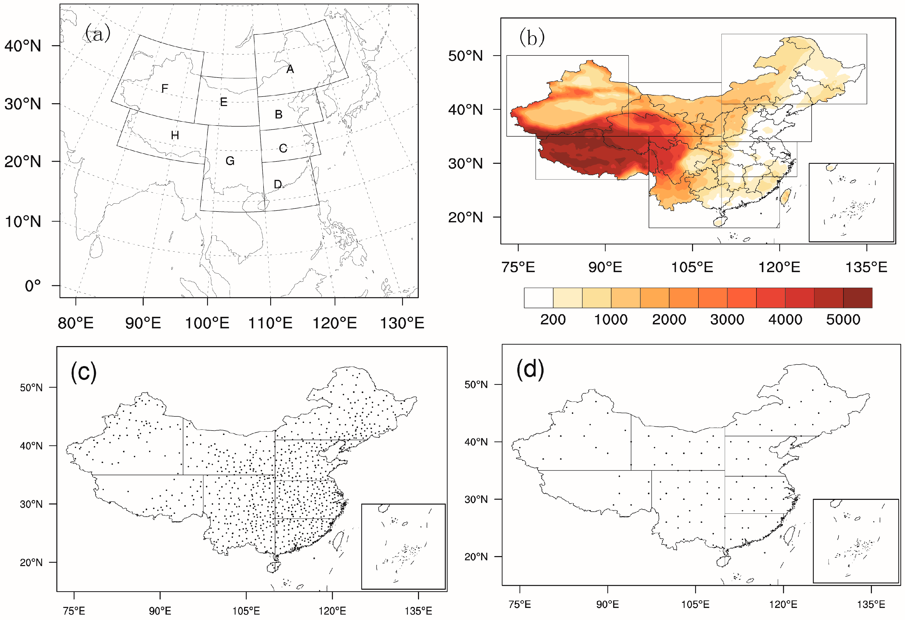
Figure 2.
Difference of simulated near-surface meteorological elements with and without nudging in summer 2010: (a–d) simulated precipitation, temperature, wind speed, and relative humidity, respectively with nudging uv; (e–h) same as a–d, but nudging θ; and (i–l) same as a–d, but nudging q.
Figure 2.
Difference of simulated near-surface meteorological elements with and without nudging in summer 2010: (a–d) simulated precipitation, temperature, wind speed, and relative humidity, respectively with nudging uv; (e–h) same as a–d, but nudging θ; and (i–l) same as a–d, but nudging q.

Figure 3.
Same as Figure 2, but for meteorological elements at 500 hPa, including: geopotential height (a,e,i); temperature (b,f,j); wind speed (c,g,k); and relative humidity (d,h,l).
Figure 3.
Same as Figure 2, but for meteorological elements at 500 hPa, including: geopotential height (a,e,i); temperature (b,f,j); wind speed (c,g,k); and relative humidity (d,h,l).

Figure 4.
Mean error (ME) of simulated near-surface meteorological elements with different nudging time: simulated precipitation (a–c); temperature (d–f); wind speed (g–i); and relative humidity (j–l), which are derived from: nudging uv (a,d,g,j); nudging θ (b,e,h,k); and nudging q (c,f,i,l).
Figure 4.
Mean error (ME) of simulated near-surface meteorological elements with different nudging time: simulated precipitation (a–c); temperature (d–f); wind speed (g–i); and relative humidity (j–l), which are derived from: nudging uv (a,d,g,j); nudging θ (b,e,h,k); and nudging q (c,f,i,l).

Figure 5.
The variation of the correlation coefficient (CC) between the simulated and observed precipitation in sub-regions A–H when various nudging times were adopted (the dashed line indicates the CC threshold passing significance t test at 0.1% significance level): (a) nudging uv; (b) nudging θ; and (c) nudging q.

Figure 6.
The variation of RATE (%) of simulated meteorological elements at standard sounding layers along with height (hPa) with different nudging time: (a) Northeast China (A); (b) North China (B); (c) East China (C); (d) South China (D); (e) East of Northwest China (E); (f) West of Northwest China (F); (g) Southwest China (G); and (h) Tibet (H).

Figure 7.
The variation of the CC between the simulated and observed geopotential height at 500 hPa in sub-regions A–H when various nudging times were adopted (the dashed line indicates the CC threshold passing significance t test at 0.1% significance level): (a) nudging uv; (b) nudging θ; and (c) nudging q.
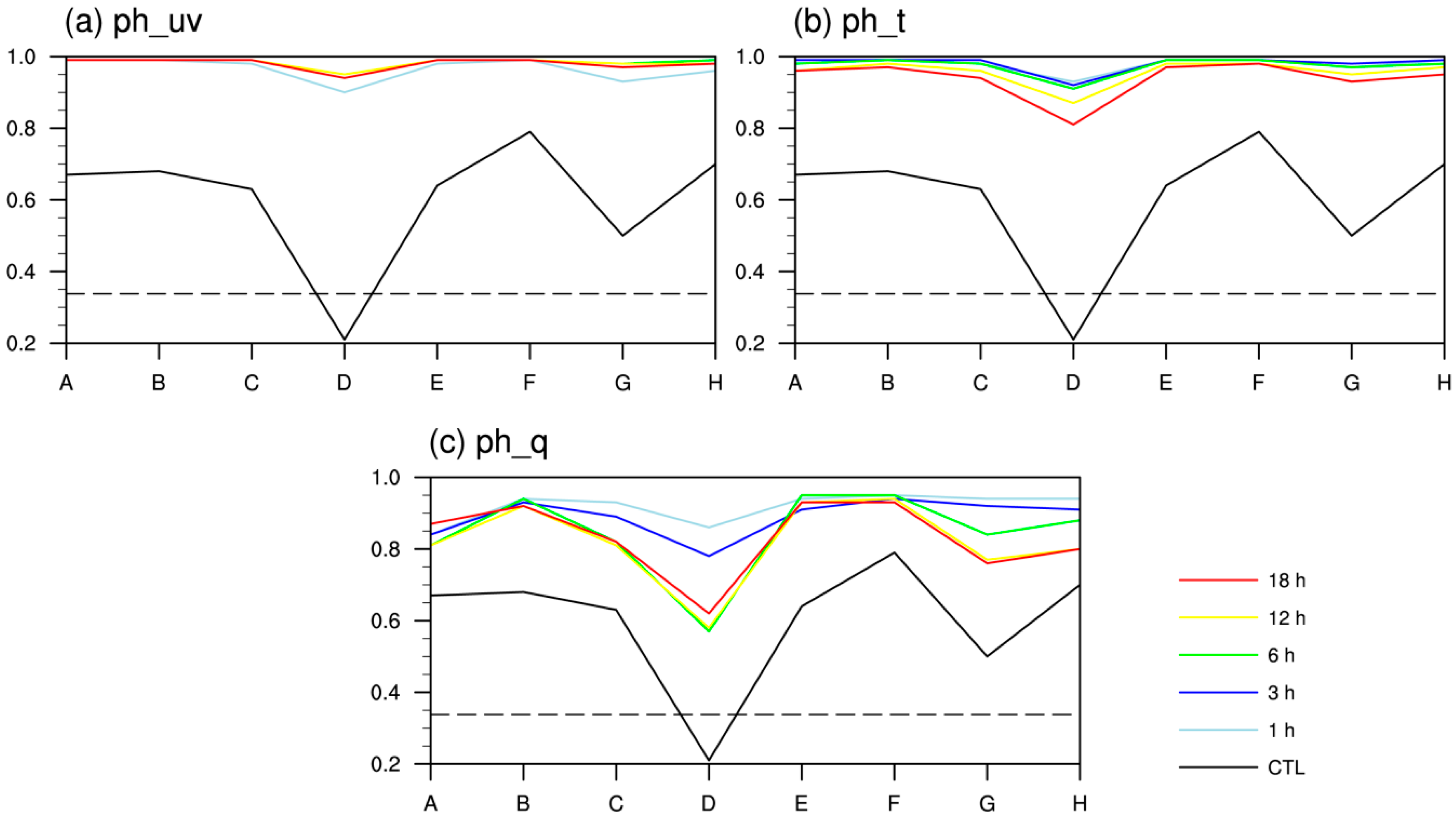
Figure 8.
The variation of CC between the simulated and observed 2 m wind with sub-regions A–H when various nudged levels were adopted (the dashed line indicates the CC threshold of significance t test at 0.1% significance level): (a) nudging uv; (b) nudging θ; and (c) nudging q.
Figure 8.
The variation of CC between the simulated and observed 2 m wind with sub-regions A–H when various nudged levels were adopted (the dashed line indicates the CC threshold of significance t test at 0.1% significance level): (a) nudging uv; (b) nudging θ; and (c) nudging q.

Figure 9.
The variation of RATE (%) of simulated meteorological elements at standard sounding layers along with height (hPa) with different nudging levels: (a) Northeast China (A); (b) North China (B); (c) East China (C); (d) South China (D); (e) East of Northwest China (E); (f) West of Northwest China (F); (g) Southwest China (G); and (h) Tibet (H).


Table 1.
Experiment design (PBL denotes planetary boundary layer, uv denotes horizontal wind, θ denotes potential temperature, and q denotes water vapor mixing ratio. Groups 1 and 2 were performed in summer 2009 and 2010, and Group 3 was performed in summer 2010).
Table 1.
Experiment design (PBL denotes planetary boundary layer, uv denotes horizontal wind, θ denotes potential temperature, and q denotes water vapor mixing ratio. Groups 1 and 2 were performed in summer 2009 and 2010, and Group 3 was performed in summer 2010).
| Group | Name | Nudged Variable | Nudging Time | Nudged Level |
|---|---|---|---|---|
| 1 | CTL | |||
| uv1 | uv | 1 h | Above the PBL | |
| t1 | θ | 1 h | Above the PBL | |
| q1 | q | 1 h | Above the PBL | |
| 2 | uv3 | uv | 3 h | Above the PBL |
| t3 | θ | 3 h | Above the PBL | |
| q3 | q | 3 h | Above the PBL | |
| uv6 | uv | 6 h | Above the PBL | |
| t6 | θ | 6 h | Above the PBL | |
| q6 | q | 6 h | Above the PBL | |
| uv12 | uv | 12 h | Above the PBL | |
| t12 | θ | 12 h | Above the PBL | |
| q12 | q | 12 h | Above the PBL | |
| uv18 | uv | 18 h | Above the PBL | |
| t18 | θ | 18 h | Above the PBL | |
| q18 | q | 18 h | Above the PBL | |
| 3 | uv_850 | uv | 1 h | Above 850 hPa |
| t_850 | θ | 1 h | Above 850 hPa | |
| q_850 | q | 1 h | Above 850 hPa | |
| uv_700 | uv | 1 h | Above 700 hPa | |
| t_700 | θ | 1 h | Above 700 hPa | |
| q_700 | q | 1 h | Above 700 hPa | |
| uv_500 | uv | 1 h | Above 500 hPa | |
| t_500 | θ | 1 h | Above 500 hPa | |
| q_500 | q | 1 h | Above 500 hPa |
Table 2.
The mean improvement rate (RATE) (%) of simulated meteorological elements near the surface with different nudging time (Bold type indicates the optimum nudging time in this region).
Table 2.
The mean improvement rate (RATE) (%) of simulated meteorological elements near the surface with different nudging time (Bold type indicates the optimum nudging time in this region).
| Scheme | A | B | C | D | E | F | G | H |
|---|---|---|---|---|---|---|---|---|
| uv1 | 24.2 | 31.0 | 36.8 | 36.0 | 27.6 | 0.6 | 24.2 | −32.5 |
| uv3 | 26.4 | 29.0 | 33.9 | 30.4 | 28.0 | 1.6 | 20.1 | −31.7 |
| uv6 | 25.9 | 27.7 | 32.0 | 27.2 | 25.8 | 0.0 | 19.5 | −33.0 |
| uv12 | 23.2 | 24.0 | 30.5 | 25.0 | 22.7 | −3.1 | 20.4 | −29.5 |
| uv18 | 20.4 | 22.0 | 29.1 | 25.7 | 19.0 | −2.7 | 20.9 | −31.0 |
| t1 | 32.0 | 41.5 | 36.3 | 25.2 | 35.9 | 22.1 | 18.7 | −33.1 |
| t3 | 38.9 | 40.7 | 48.6 | 38.8 | 38.2 | 23.3 | 31.1 | −35.2 |
| t6 | 34.2 | 38.1 | 45.8 | 33.8 | 34.1 | 20.8 | 28.1 | −38.5 |
| t12 | 29.3 | 31.3 | 39.2 | 29.4 | 27.7 | 18.0 | 23.4 | −38.4 |
| t18 | 26.2 | 28.1 | 36.4 | 31.1 | 23.9 | 16.1 | 23.6 | −33.6 |
| q1 | −14.3 | 24.4 | 37.8 | 36.4 | 25.0 | −10.7 | 33.2 | −19.0 |
| q3 | −22.5 | 17.6 | 33.5 | 34.5 | 22.5 | −9.8 | 32.5 | −15.6 |
| q6 | −32.4 | 11.9 | 27.9 | 31.2 | 23.6 | −11.7 | 28.8 | −12.3 |
| q12 | −14.6 | 7.6 | 23.0 | 27.0 | 21.1 | −7.4 | 24.5 | −10.1 |
| q18 | −6.7 | 10.2 | 20.1 | 22.5 | 9.0 | −10.6 | 18.6 | −16.2 |
Table 3.
Same as Table 2, but for simulations at sounding standard layers.
Table 3.
Same as Table 2, but for simulations at sounding standard layers.
| Scheme | A | B | C | D | E | F | G | H |
|---|---|---|---|---|---|---|---|---|
| uv1 | 41.5 | 42.7 | 39.7 | 28.7 | 40.2 | 23.8 | 30.7 | 25.0 |
| uv3 | 42.0 | 43.1 | 40.3 | 33.8 | 41.4 | 25.1 | 31.4 | 29.2 |
| uv6 | 40.9 | 42.3 | 39.7 | 34.2 | 40.9 | 24.0 | 30.9 | 28.8 |
| uv12 | 38.8 | 40.9 | 38.4 | 32.6 | 38.5 | 21.3 | 29.1 | 26.2 |
| uv18 | 37.3 | 39.8 | 37.2 | 31.2 | 36.1 | 19.1 | 27.6 | 24.3 |
| t1 | 49.2 | 48.3 | 48.4 | 41.1 | 49.9 | 38.0 | 43.2 | 36.1 |
| t3 | 50.6 | 51.3 | 52.3 | 44.2 | 50.0 | 39.2 | 45.4 | 38.7 |
| t6 | 49.6 | 50.6 | 51.2 | 43.5 | 46.2 | 37.3 | 43.7 | 36.6 |
| t12 | 45.8 | 45.4 | 45.0 | 39.3 | 40.3 | 33.7 | 38.6 | 31.2 |
| t18 | 43.0 | 41.9 | 41.5 | 36.3 | 37.1 | 30.8 | 35.8 | 28.6 |
| q1 | 21.4 | 35.2 | 38.0 | 36.2 | 29.7 | 16.8 | 30.8 | 28.5 |
| q3 | 18.1 | 29.2 | 31.9 | 32.5 | 26.9 | 14.9 | 26.6 | 24.9 |
| q6 | 13.3 | 23.6 | 27.7 | 28.6 | 23.9 | 11.8 | 24.3 | 22.0 |
| q12 | 15.0 | 22.2 | 24.3 | 26.3 | 20.7 | 7.4 | 20.4 | 14.7 |
| q18 | 15.4 | 20.1 | 23.7 | 23.7 | 16.2 | −3.4 | 16.7 | 10.9 |
Table 4.
RATE (%) of simulated near-surface meteorological elements with different nudged levels.
| Scheme | A | B | C | D | E | F | G | H |
|---|---|---|---|---|---|---|---|---|
| uv1 | 24.2 | 31.0 | 36.8 | 36.0 | 27.6 | 0.6 | 24.2 | −32.5 |
| uv_500 | 14.8 | 15.1 | 20.2 | 23.5 | 13.0 | −2.8 | 26.6 | −34.3 |
| uv_700 | 19.0 | 22.0 | 25.7 | 26.1 | 20.9 | 1.2 | 29.1 | −23.9 |
| uv_850 | 25.2 | 26.9 | 30.0 | 28.4 | 28.4 | 3.0 | 34.4 | −27.0 |
| t_1 | 32.0 | 41.5 | 36.3 | 25.2 | 35.9 | 22.1 | 18.7 | −33.1 |
| t_500 | 12.3 | 8.4 | 14.0 | 27.2 | 11.9 | −4.1 | 25.0 | −15.4 |
| t_700 | 26.6 | 23.2 | 43.9 | 37.2 | 32.4 | 2.9 | 35.5 | −29.3 |
| t_850 | 32.9 | 38.3 | 46.8 | 33.7 | 38.1 | 23.1 | 28.9 | −33.7 |
| q1 | −14.3 | 24.4 | 37.8 | 36.4 | 25.0 | −10.7 | 33.2 | −19.0 |
| q_500 | −9.9 | −26.4 | −10.0 | 2.3 | −9.2 | −22.9 | 8.3 | −25.8 |
| q_700 | −2.5 | −1.6 | −6.2 | 11.4 | −3.0 | −27.4 | 5.3 | −9.4 |
| q_850 | −1.5 | 22.0 | 33.3 | 25.5 | 18.7 | −19.7 | 21.7 | −3.5 |
Table 5.
Same as Table 4, but for the simulations at sounding standard layers.
Table 5.
Same as Table 4, but for the simulations at sounding standard layers.
| Scheme | A | B | C | D | E | F | G | H |
|---|---|---|---|---|---|---|---|---|
| uv1 | 41.5 | 42.7 | 39.7 | 28.7 | 40.2 | 23.8 | 30.7 | 25.0 |
| uv_500 | 33.0 | 33.6 | 30.8 | 23.6 | 34.2 | 21.3 | 22.5 | 18.6 |
| uv_700 | 38.6 | 38.7 | 34.6 | 27.4 | 39.8 | 24.8 | 25.5 | 22.6 |
| uv_850 | 40.6 | 41.4 | 38.1 | 27.5 | 41.4 | 25.0 | 28.7 | 27.0 |
| t_1 | 49.2 | 48.3 | 48.4 | 41.1 | 49.9 | 38.0 | 43.2 | 36.1 |
| t_500 | 31.0 | 29.0 | 35.1 | 29.9 | 35.4 | 18.3 | 26.9 | 25.9 |
| t_700 | 42.4 | 41.5 | 46.7 | 36.9 | 43.3 | 25.8 | 38.6 | 31.9 |
| t_850 | 47.0 | 46.4 | 49.1 | 41.2 | 49.2 | 37.4 | 44.2 | 35.5 |
| q1 | 21.4 | 35.2 | 38.0 | 36.2 | 29.7 | 16.8 | 30.8 | 28.5 |
| q_500 | 1.5 | 0.6 | 7.9 | 10.2 | −3.5 | −15.5 | 5.5 | 0.4 |
| q_700 | 17.9 | 16.9 | 15.5 | 17.8 | 16.8 | −11.6 | 10.2 | 3.5 |
| q_850 | 25.0 | 32.5 | 34.2 | 30.1 | 29.5 | 7.0 | 25.3 | 25.5 |
Table 6.
Same as Table 2, except that the simulation results from 2009 were adopted (* denotes the optimum nudging time in 2010).
Table 6.
Same as Table 2, except that the simulation results from 2009 were adopted (* denotes the optimum nudging time in 2010).
| Scheme | A | B | C | D | E | F | G | H |
|---|---|---|---|---|---|---|---|---|
| uv1 | 40.2 | 37.8 * | 37.5 * | 37.6 * | 24.2 | 20.3 | 16.5 * | −28.6 |
| uv3 | 41 * | 36.1 | 33 | 33 | 24.5 * | 22 * | 14.2 | −27.6 |
| uv6 | 38.3 | 33.7 | 29.9 | 30.8 | 24.5 | 21.9 | 15 | −26.2 |
| uv12 | 34.7 | 30.8 | 26 | 27.5 | 22.8 | 21.3 | 17.1 | −22.6 |
| uv18 | 31.7 | 29 | 25.5 | 25.5 | 20.5 | 21.6 | 18 | −21 |
| t1 | 45.1 | 43.7 * | 35.7 | 18.1 | 32.5 | 34.7 | 4.2 | −26.3 |
| t3 | 50.1 * | 45.7 | 48.1 * | 35 * | 35.2 * | 36.5 * | 22.1 * | −24.8 |
| t6 | 49.2 | 46.2 | 49.6 | 34.6 | 31.9 | 36.1 | 23 | −23.1 |
| t12 | 45.5 | 42.3 | 47.1 | 35.9 | 32.9 | 34.8 | 20.1 | −20.6 |
| t18 | 44.2 | 41.5 | 45.8 | 35 | 30.6 | 33.8 | 19.5 | −20.4 |
| q1 | −10.8 | 26.4 * | 44.7 * | 33.9 * | 23.6 * | 27.8 | 33.5 * | −13.5 |
| q3 | −13.8 | 27.3 | 41.9 | 32.4 | 26.2 | 28.3 | 30.3 | −11.7 |
| q6 | −13.3 | 27.1 | 39.3 | 30.4 | 22.4 | 27.5 | 25.2 | −12.3 |
| q12 | 1.7 | 24.5 | 31 | 27.8 | 25.2 | 28.4 | 17 | −9 |
| q18 | 7.9 | 19.7 | 27.3 | 25 | 18.3 | 26.7 | 15.9 | −9.1 |
Table 7.
Same as Table 3, except that the simulation results from 2009 were adopted (* denotes the optimum nudged level in 2010).
Table 7.
Same as Table 3, except that the simulation results from 2009 were adopted (* denotes the optimum nudged level in 2010).
| Scheme | A | B | C | D | E | F | G | H |
|---|---|---|---|---|---|---|---|---|
| uv1 | 42.5 | 46.2 | 39 | 38.6 | 35.5 | 26 | 29.2 | 28.9 |
| uv3 | 42.6 * | 46.9 * | 39 * | 41 | 36.9 * | 27.6 * | 32 * | 34.2 * |
| uv6 | 40.9 | 46 | 38.7 | 41.1 * | 36.8 | 27.4 | 31.7 | 34.8 |
| uv12 | 38.7 | 43.7 | 37.3 | 39.6 | 35.4 | 26 | 29.7 | 33.7 |
| uv18 | 37.8 | 42.7 | 36.5 | 38.3 | 34.6 | 24.8 | 28.6 | 32.2 |
| t1 | 53.8 | 50.7 | 44.4 | 43.9 | 39.6 | 37.6 | 44.5 | 40.2 |
| t3 | 55.4 * | 52.6 * | 47.6 * | 46.4 * | 41.6 * | 39.3 * | 46.1 * | 40.9 * |
| t6 | 53.7 | 52.1 | 47 | 45.5 | 41 | 38.3 | 45.5 | 40.9 |
| t12 | 47.5 | 47.3 | 45.6 | 42.8 | 37.8 | 35.3 | 41.9 | 39.5 |
| t18 | 45.2 | 44.7 | 43.7 | 41.2 | 37.1 | 33 | 41 | 38.4 |
| q1 | 22.2 * | 33.2 * | 37 * | 36.4 * | 28.4 * | 27.7 * | 30.1 * | 34 * |
| q3 | 18.6 | 30.8 | 34.5 | 33.2 | 25.2 | 25.1 | 27.2 | 32 |
| q6 | 15.4 | 28.1 | 31.3 | 29.6 | 22 | 21.3 | 25.2 | 28.8 |
| q12 | 17.3 | 24.5 | 25.3 | 23.7 | 21.6 | 16.4 | 19.4 | 25.4 |
| q18 | 17.2 | 23.1 | 21.7 | 22 | 18.9 | 11.3 | 17 | 21.6 |
© 2017 by the authors. Licensee MDPI, Basel, Switzerland. This article is an open access article distributed under the terms and conditions of the Creative Commons Attribution (CC BY) license (http://creativecommons.org/licenses/by/4.0/).
Share and Cite
MDPI and ACS Style
Mai, X.; Ma, Y.; Yang, Y.; Li, D.; Qiu, X. Impact of Grid Nudging Parameters on Dynamical Downscaling during Summer over Mainland China. Atmosphere 2017, 8, 184. https://doi.org/10.3390/atmos8100184
AMA Style
Mai X, Ma Y, Yang Y, Li D, Qiu X. Impact of Grid Nudging Parameters on Dynamical Downscaling during Summer over Mainland China. Atmosphere. 2017; 8(10):184. https://doi.org/10.3390/atmos8100184
Chicago/Turabian StyleMai, Xiaoping, Yuanyuan Ma, Yi Yang, Deqin Li, and Xiaobin Qiu. 2017. "Impact of Grid Nudging Parameters on Dynamical Downscaling during Summer over Mainland China" Atmosphere 8, no. 10: 184. https://doi.org/10.3390/atmos8100184
Note that from the first issue of 2016, this journal uses article numbers instead of page numbers. See further details here.