1. Introduction
With over 600 active coal-fired power plants in the US, 39% of the country’s total electricity generation is attributed to coal (Available online:
http://www.eia.gov). While these plants may bring jobs and prosperity to their surrounding regions, they also emit dangerous pollutants into the atmosphere. According to the US Environmental Protection Agency (EPA) National Emissions Inventory, coal-fired power plants emit sulfur dioxide, oxides of nitrogen and particulate matter into the atmosphere. They also emit 84 of the 187 Hazardous Air Pollutants (HAP) regulated by the US EPA [
1]. In addition to the stack emissions from the coal-fired power plant, coal handling may also emit pollutants into the atmosphere and thus degrade the air quality in the vicinity near the power plant [
2]. Several studies have been conducted on the relationship between particulate matter and emissions from coal-fired power plants [
2,
3,
4,
5,
6,
7,
8,
9,
10,
11,
12,
13,
14]. Particulate matter measured near a coal-fired power plant is known to contain a number of harmful chemicals that are present in coal and are also known to have carcinogenic properties, such as antimony, arsenic, beryllium, cadmium, chromium, cobalt, lead, manganese, mercury, nickel, selenium and polycyclic organic matter (POM) [
2,
3,
4]. All of these chemicals are known to be hazardous and are thus regulated by the US EPA as HAPs under the Clean Air Act, as amended in 1990 [
15]. The emission of these pollutants into the atmosphere is known to be dangerous to both human health and welfare. Exposure to high concentrations of HAPs can lead to a number of adverse health effects such as damage to the eyes, skin, lungs, kidneys and the nervous system, and can even cause cancer, pulmonary disease and cardiovascular disease [
14,
16]. Particulate matter (PM
2.5), which is particulate matter with an aerodynamic diameter of 2.5 microns or less, is also a dangerous atmospheric pollutant due to its small size, which can travel deep into people’s lungs and lead to a number of severe health effects. Elevated concentrations of PM
2.5 are known to be associated with cardiovascular issues (heart disease, heart attacks, etc.) as well as respiratory issues, reproductive issues and even cancer [
16,
17]. In addition to harming human health, coal-fired power plants can also lead to a number of environmental impacts as well, such as acidification of the environment, bioaccumulation of toxic metals, the contamination of water sources, reduced visibility due to haze as well as degradation of buildings and monuments.
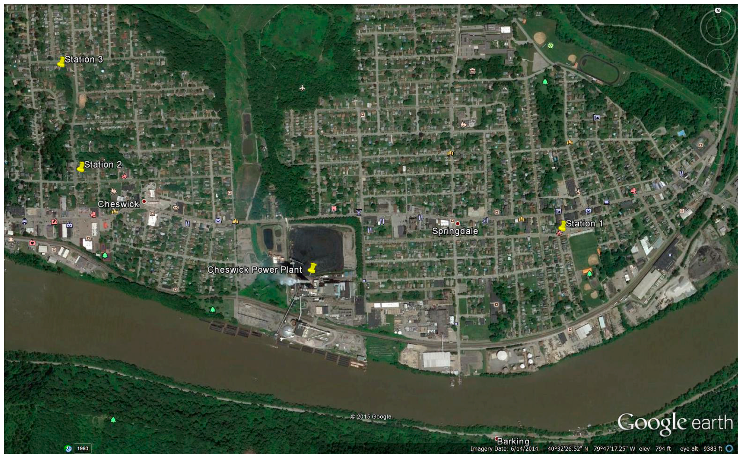
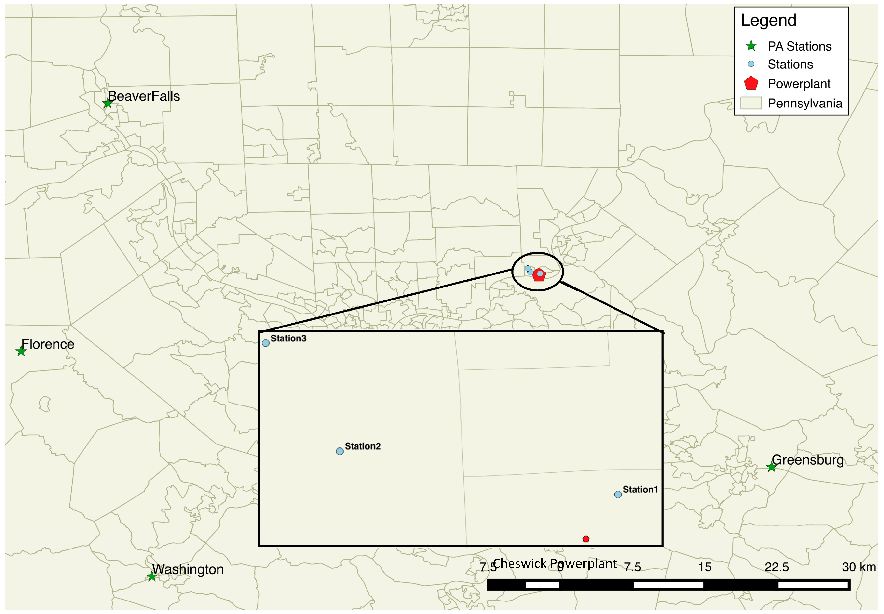
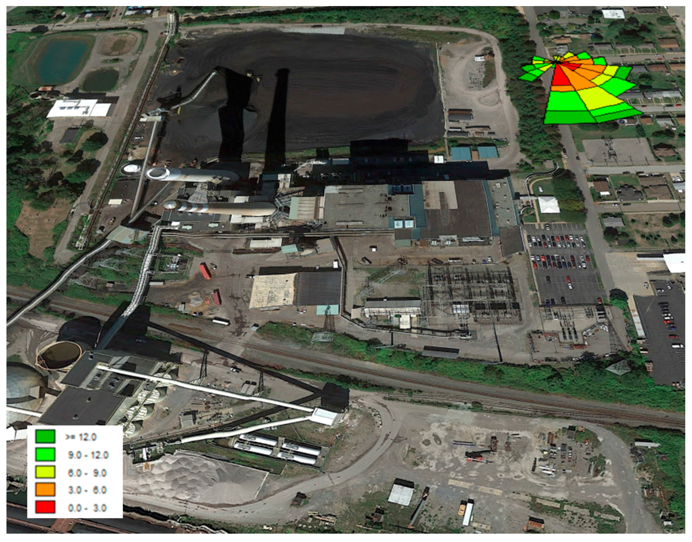
The Cheswick Power Plant is located in the southwestern part of Pennsylvania along the Allegheny River right between the boroughs of Springdale (40.5414° N, 79.7821° W) and Cheswick (40.5416° N, 79.8002° W) (
Figure 1). While the Cheswick Power Plant has brought economic benefits to the small boroughs of Springdale and Cheswick, PA, the plant also brought with it a multitude of harmful effects on both human health and welfare. According to the Allegheny County Health Department's Point Source Emissions Inventory Report, the Cheswick Power Station is the largest point source emitter of both criteria pollutants and hazardous air pollutants (HAP) in Allegheny County, PA [
18]. In 2006, the plant was listed as the 17th Dirtiest Power Plant for sulfur dioxide [
1]. In 2010, the plant once again made headlines, ranking 41st in the Top Power Plant Hydrochloric Acid Emitters and 91st in the Top US Power Plant Lead Emitters [
19]. Since then, significant efforts have been made to reduce emissions [
18]. Overall, emissions of carbon monoxide and sulfur dioxide did decrease in 2011, while emissions of nitrogen oxides, particulate matter, NO
x, and volatile organic compounds (VOC) increased [
18]. However, the plant remains Allegheny County’s largest point source emitter of both criteria pollutants and hazardous air pollutants. The objective of this study was to measure the air quality at three different locations within the two boroughs surrounding the power plant in order to determine concentrations of both PM
2.5 and PM
10 due to emissions from the power plant. Particulate matter measurements measured by the PA Department of Environmental Protection (DEP) were also analyzed for the study period and compared against the measurements taken for this study.
3. Results and Discussion
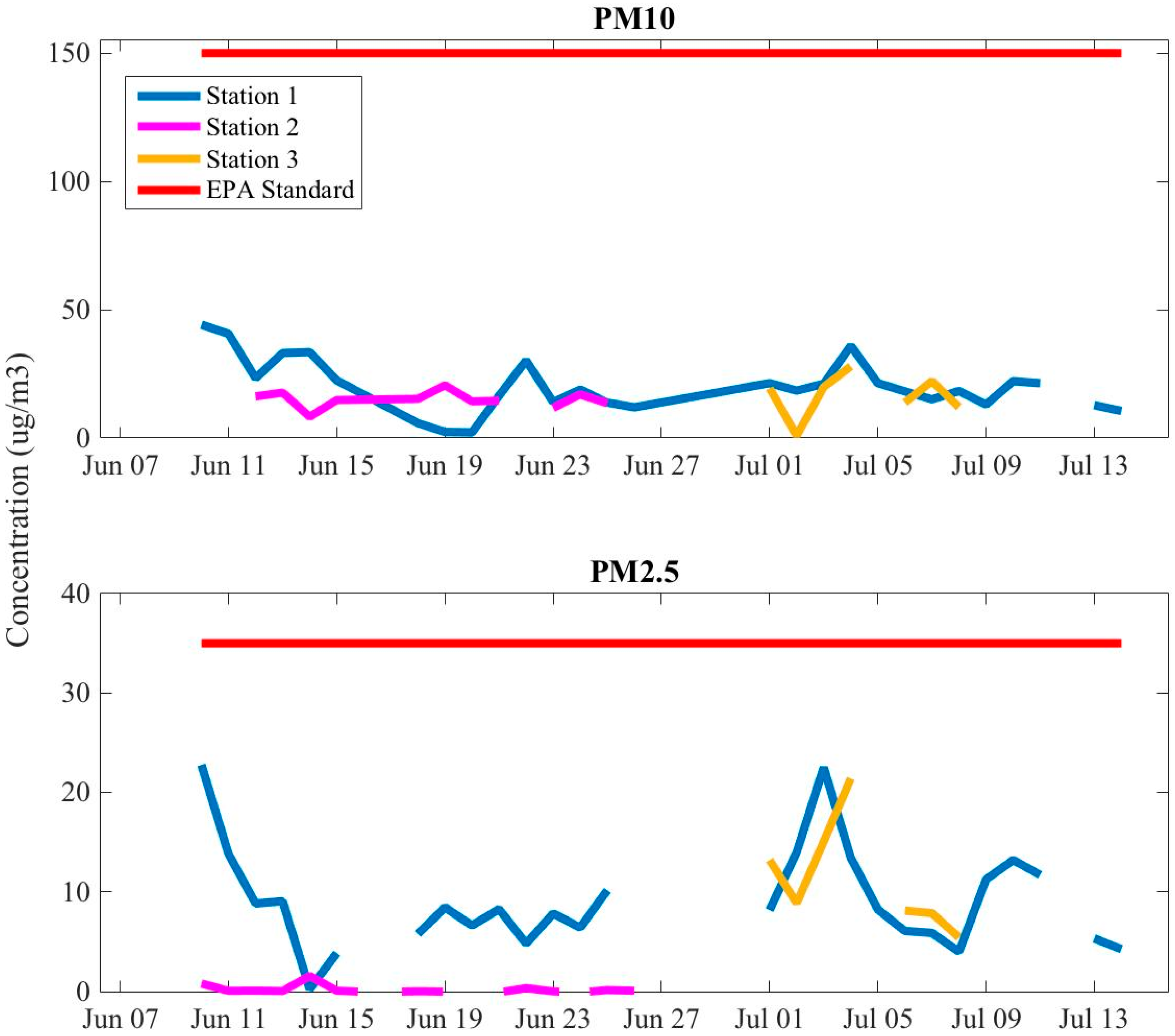
The observed average 24-hour concentrations of both PM
2.5 (0.02–22.76 μg m
−3) and PM
10 (0.9−44.15 μg m
−3) from the NCSU monitoring sites were found to be lower than the US EPA National Ambient Air Quality Standard of 35 μg m
−3 and 150 μg m
−3, respectively (
Figure 3).
The average concentrations of PM
10 observed during the periods were 20.5 ± 10.2 μg m
−3 (Station 1), 16.1 ± 4.9 μg m
−3 (Station 2) and 16.5 ± 7.1 μg m
−3 (Station 3). The average concentrations of PM
2.5 observed at the stations were 9.1 ± 5.1 μg m
−3 (Station 1), 0.2 ± 0.4 μg m
−3 (Station 2) and 11.6 ± 4.8 μg m
−3 (Station 3). Station 1 observed the maximum concentrations of both PM
2.5 (22.76 μg m
−3) and PM
10 (44.15 μg m
−3 μg m
−3). While Station 3 also observed higher concentrations of particulate matter (both PM
2.5 and PM
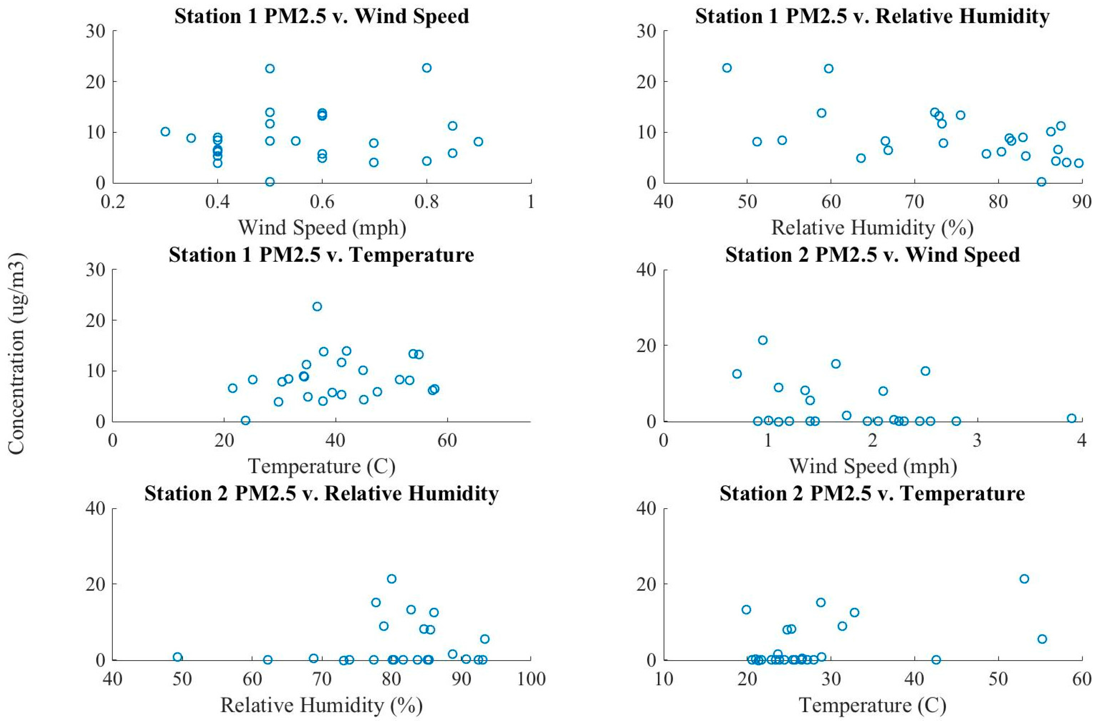
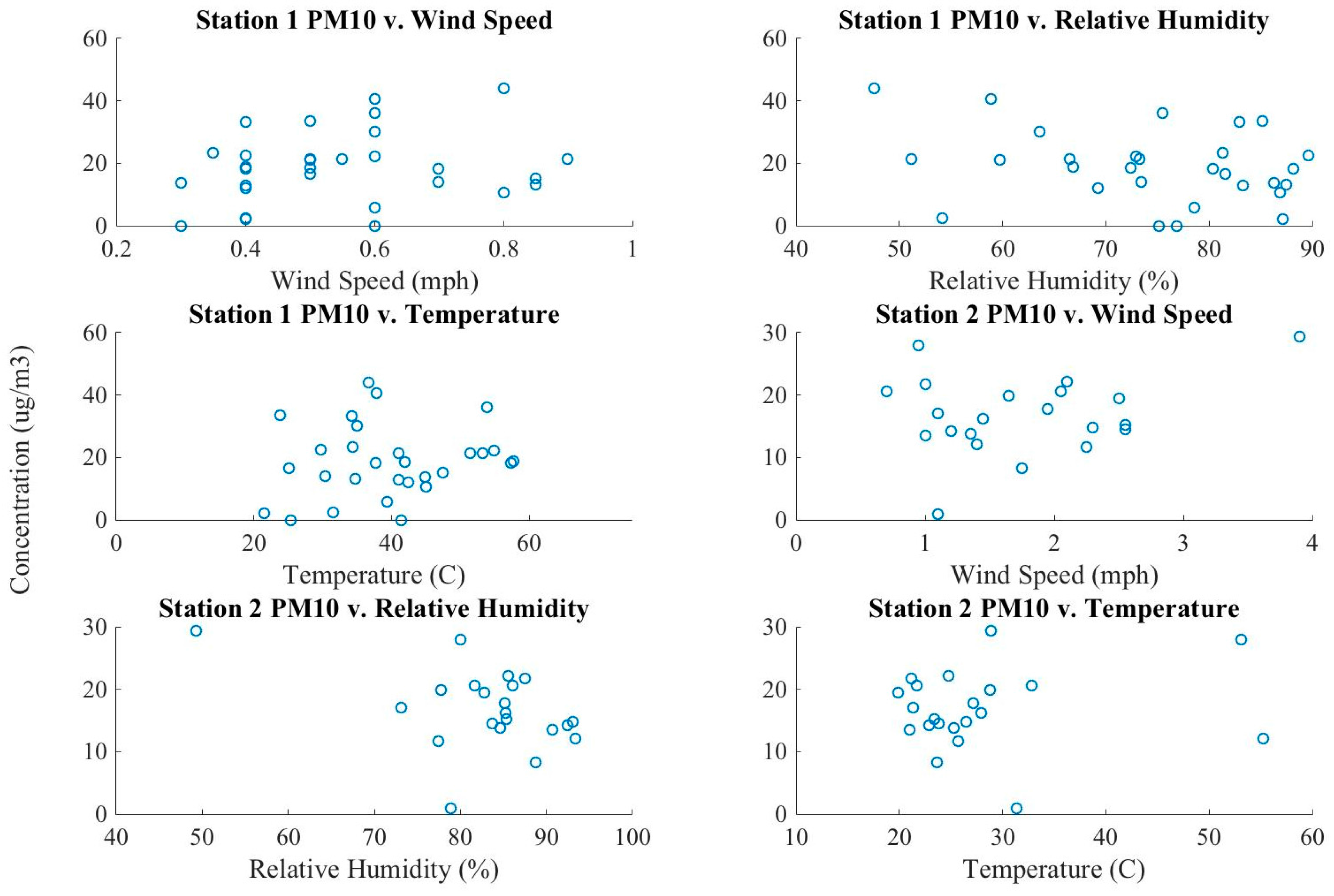
10), the results of a t test (at α = 0.05) indicated that the concentrations at Station 1 were indeed higher than those observed at Stations 2 and 3. There are several plausible causes for this: the location of Station 1 versus Stations 2 and 3 in relation to the meteorological conditions as well as additional potential sources of particulate matter into the atmosphere (i.e., traffic emissions, roadway dust, transport). Concentrations of particulate matter tended to be higher when conditions were warm and sunny. Conversely, the lowest concentrations of particulate matter were primarily observed during rainy conditions. This was expected due to the removal of the particulates from the atmosphere through wet deposition. However, there were a few days where elevated concentrations were observed when the plant was running during rainy conditions. This may have resulted from the stability of the atmosphere in these conditions, which allows for the atmospheric accumulation of particulate matter. Nevertheless, comparisons of particulate matter concentrations with meteorological conditions (
Figure 4 and
Figure 5) failed to show any strong correlations.
When comparing the median wind speed versus the concentration of PM10 at Stations 1 and 2, positive correlations of 0.2 and 0.27, respectively, were observed. When comparing the median relative humidity with the concentration of PM10, negative correlations of 0.3 and 0.44 were observed, respectively, while minor positive correlations of 0.08 and 0.12 were observed for temperature and concentration at Stations 1 and 2, respectively. When comparing meteorological conditions with concentrations of PM2.5 at Stations 1 and 2, a negative correlation of 0.32 between wind speed and concentration of PM2.5 was observed at Station 2 while Station 1 observed a positive correlation of 0.12. The strongest meteorological correlation was a negative correlation of −0.56 between relative humidity and the concentration of PM2.5 at Stations 1, which is nominally downwind from the plant. In contrast, the correlation between relative humidity and PM2.5 was weakly positive, at 0.09, for Station 2. Positive correlations of 0.54 and 0.46 were observed when comparing temperature versus concentrations of PM2.5 at Stations 1 and 2, respectively. However, when considering these correlations, it is important to acknowledge the short sample period and thus small sample.
The median wind direction at upwind versus downwind stations was compared with the average 24-hour concentrations of particulate matter, where the categorizations of upwind and downwind were denoted based on the daily median wind direction. The results of a t test provide p = 0.5 and p = 0.4, for concentrations of PM10 and PM2.5, respectively, which suggests that the relationship is not statistically significant.
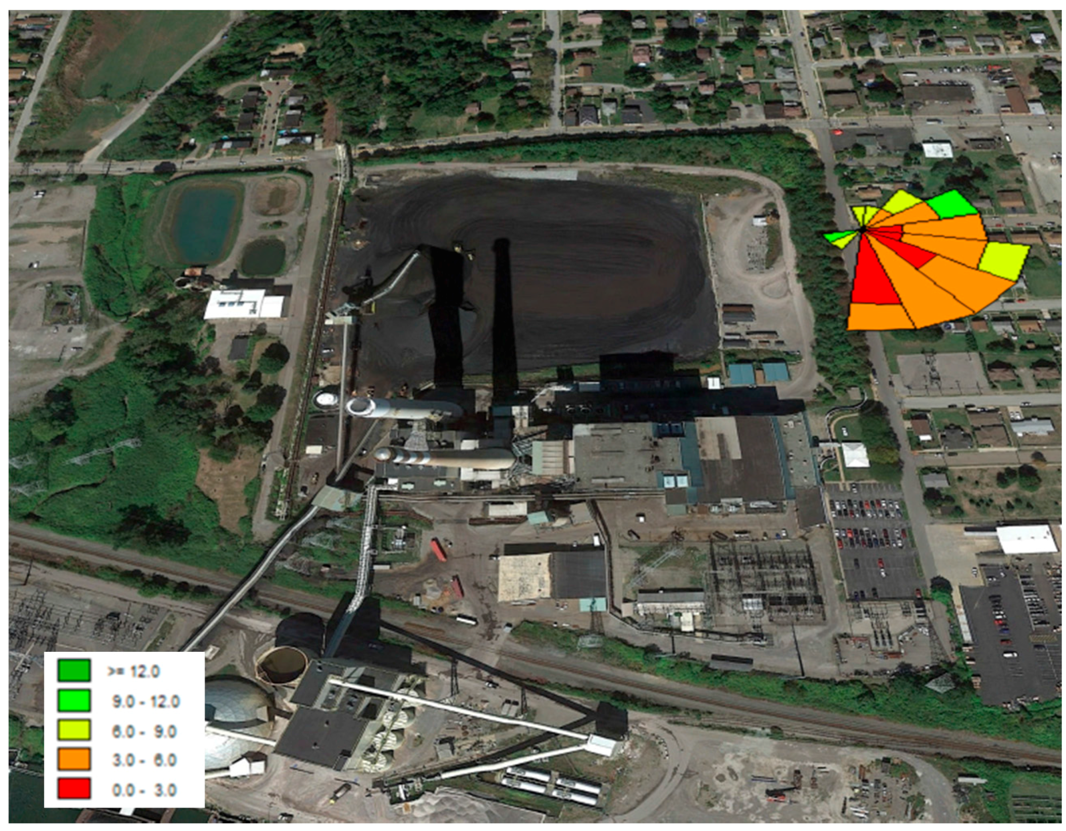
Despite the fact that the median wind direction was not significantly correlated with the concentrations of particulate matter, the local hourly wind direction likely did impact concentrations of particulate matter. Furthermore, it is likely that some of the relatively high concentrations of both particulate matter observed at Station 1 were found to have come from the direction of the coal site on the power plant’s property (
Figure 6 and
Figure 7). In addition to observing elevated concentrations coming directly from the plant, elevated concentrations of both PM
2.5 and PM
10 were also observed coming from other directions. This can likely be attributed to a number of sources, such as emissions from vehicles, road dust. In addition, the elevated concentrations can also be attributed to transport due to local and regional meteorological phenomena. Furthermore, fairly elevated concentrations of PM
10 are observed at faster wind speeds. While wind speeds would generally reduce ambient concentrations of particulate matter in the atmosphere, the observed elevated concentrations could simply be due to an emission source located extremely close to the monitoring site (i.e., a stalled truck on the side of the road).
In contrast to this, neither Stations 2 nor 3 (not pictured) showed extremely high concentrations coming from the power plant. However, this is not entirely surprising for two reasons: the first reason is that the winds were primarily such that those stations were upwind of the power plant and that both of these stations were twice as far as Station 1 for the plant, thus allowing for some dispersion of pollutants emitted from the plant and the coal site to occur.
In addition to this, concentrations of both PM
2.5 and PM
10 were compared at calm wind conditions (median wind speeds less than 1 kt) and non-calm wind conditions (
Table 1). When comparing average concentrations of PM
2.5 during calm winds (9.29 ± 5.59 µg m
−3) with average concentrations during not calm winds (3.53 ± 5.18 µg m
−3), it is clear that the average concentrations during calm winds are higher than the average concentrations during not calm winds. Similarly, average concentrations of PM
10 observed during calm winds (19.83 ± 10.29 µg m
−3) was higher than the average concentrations observed when the winds were not calm (16.25 ± 4.87 µg m
−3). Two
t tests were also conducted in order to determine whether or not the comparison between concentrations of PM
2.5 and PM
10 during calm and not calm winds was statistically significant. The results of the t tests provide
p = 0.052 and
p = 0.001, for concentrations of PM
10 and PM
2.5, respectively. This suggests that while the comparison between concentrations of PM
2.5 during calm and not calm winds is statistically significant, the comparison for concentrations of PM
10 is not quite statistically significant.
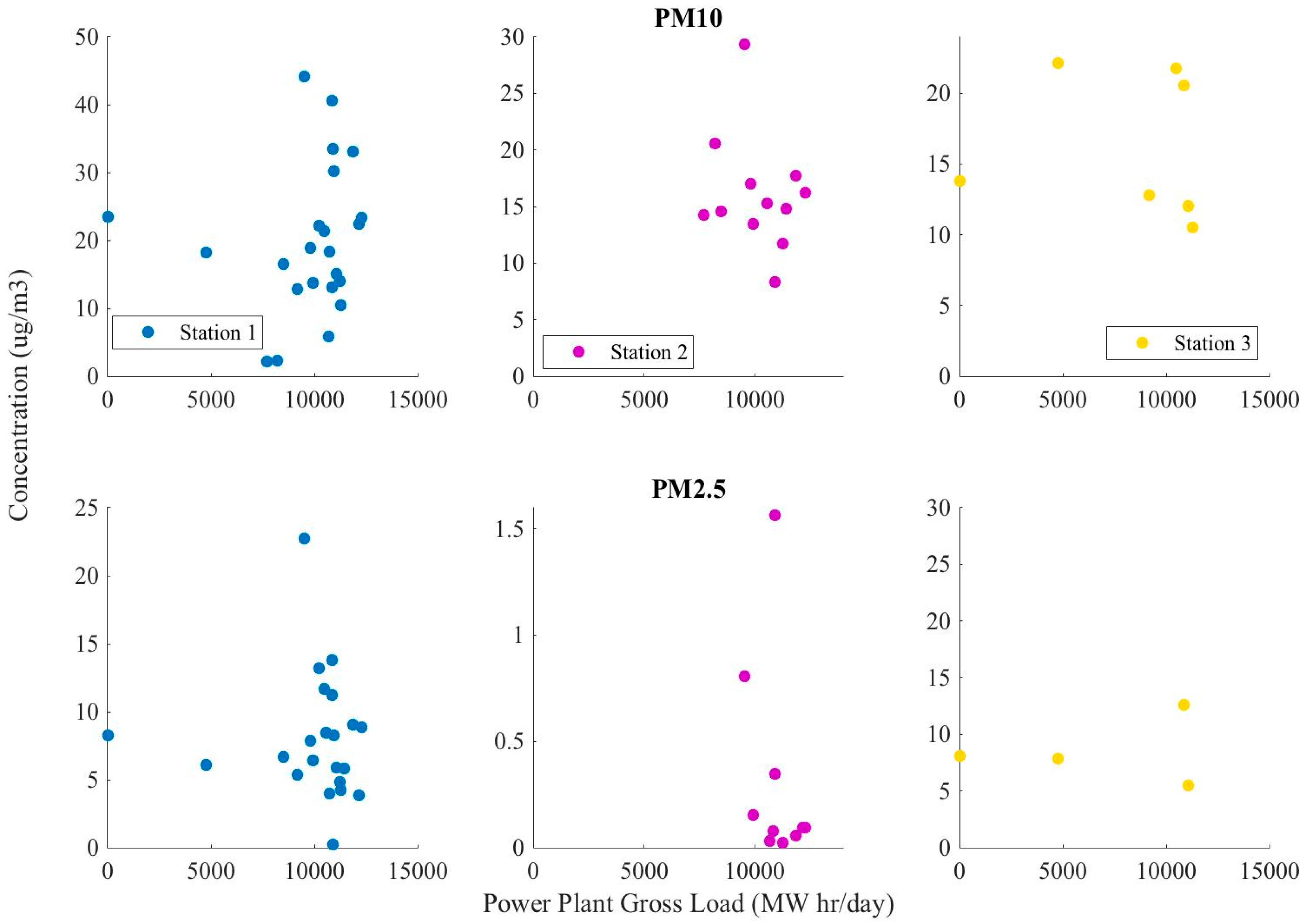
Concentrations of particulate matter were also compared with the plant’s gross load during the period (power plant gross load obtained via: EPA. Available online:
http://www.ampd.epa.gov/ampd).
Figure 8 compares the Cheswick Power Plant’s daily gross load with the daily 24-hour average concentration of PM
10 and PM
2.5. When comparing the daily gross load with the particulate matter concentrations, the correlation coefficients (ranging between −0.23 and 0.15) suggest that the concentrations of particulate matter at each station are not statistically correlated with the plant gross load.
Five PM
10 samples and five PM
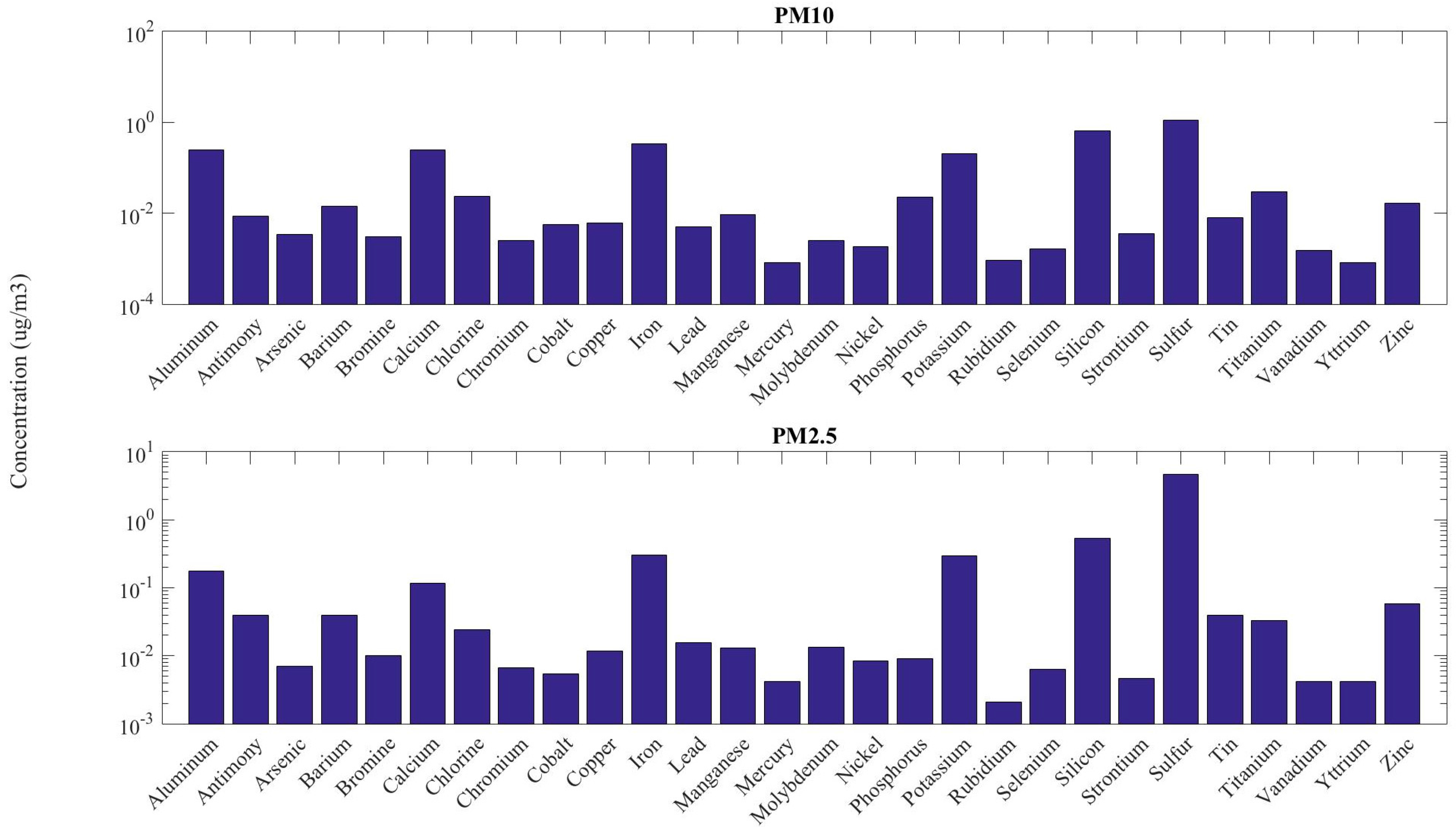
2.5 samples were subjected to XRF and IC analysis. The XRF analysis represents the PM samples as elements, while the IC analysis represents the PM samples as ions. When comparing the results of the analyses, it is evident that they are consistent. The results of the XRF analysis (
Figure 9) showed that the primary constituents of PM
10 are sulfur (0.66–1.77 μg m
−3), silicon (0.14–2.47 μg m
−3), aluminum (0.03–1.06 μg m
−3) and iron (0.08–0.95 μg m
−3). Similarly, the primary constituents of PM
2.5 were found to be sulfur (0.41–1.17 μg m
−3), silicon (0.02–0.23 μg m
−3) and iron (0.03–0.06 μg m
−3). Particulate matter is typically composed of a complex mixture of chemicals that are strongly dependent on source characteristics. Inorganic analysis of the particulate matter revealed the presence of antimony, arsenic, beryllium, cadmium, chromium, cobalt, lead, manganese, mercury, nickel and selenium (
Figure 9). All of these metals present in the PM samples are known to be present in coal [
21]. While these elements are all found within coal and coal ash, they are also present in crustal material. Based on the small number of samples analyzed, it was not possible to discern differences between the upwind and downwind samples. The highest concentration of sulfur observed in a sample during the period was observed at Station 1. In this case, it is possible that this can be attributed to the coal pit, which is located less than half of a mile away from the station. However, it is also important to note that there are other coal-fired power plants located within 50 miles of the Cheswick Power plant, which could also contribute to the elevated sulfur concentrations.
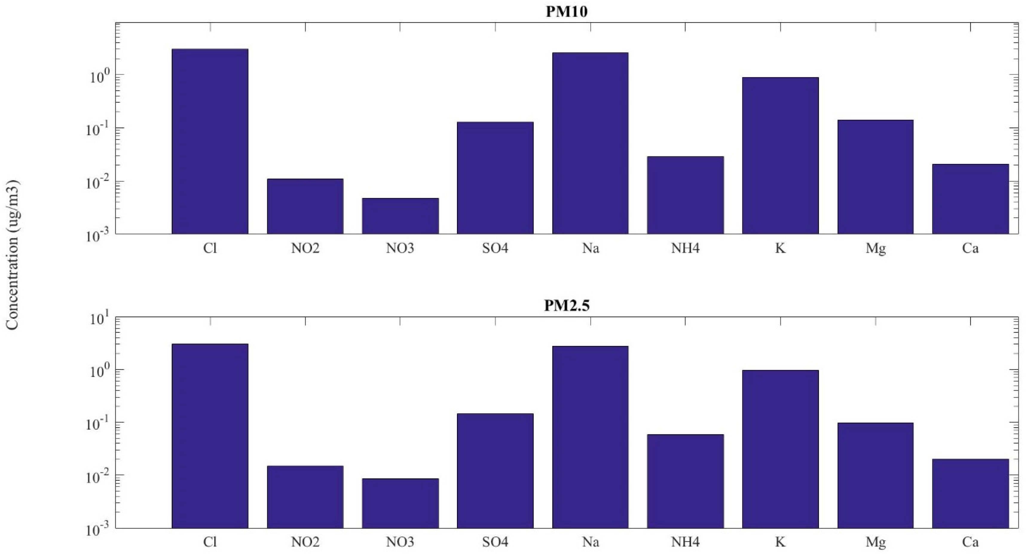
The results of the IC analysis (
Figure 10) showed that the dominant species of particulate matter in this region are primarily sulfate, nitrate and ammonium. Within the PM
2.5 samples analyzed, concentrations of sulfate ranged from 2.31 μg m
−3 to 3.08 μg m
−3, nitrate concentrations ranged from 0.03 μg m
−3 to 0.58 μg m
−3, and concentrations of ammonium ranged from 0.82 μg m
−3 to 1.15 μg m
−3. Within the analyzed PM
10 samples, concentrations of sulfate ranged from 1.05 μg m
−3 to 4.73 μg m
−3, concentrations of nitrate ranged from 0.01 μg m
−3 to 0.22 μg m
−3 and concentrations of ammonium ranged from 0.38 μg m
−3 to 1.69 μg m
−3. As described above, it was not possible to discern differences between the upwind and downwind samples based on the small sample size. It is also important to note that sulfate, nitrate and ammonium are also common constituents of particulate matter and thus cannot be attributed entirely to the power plant.
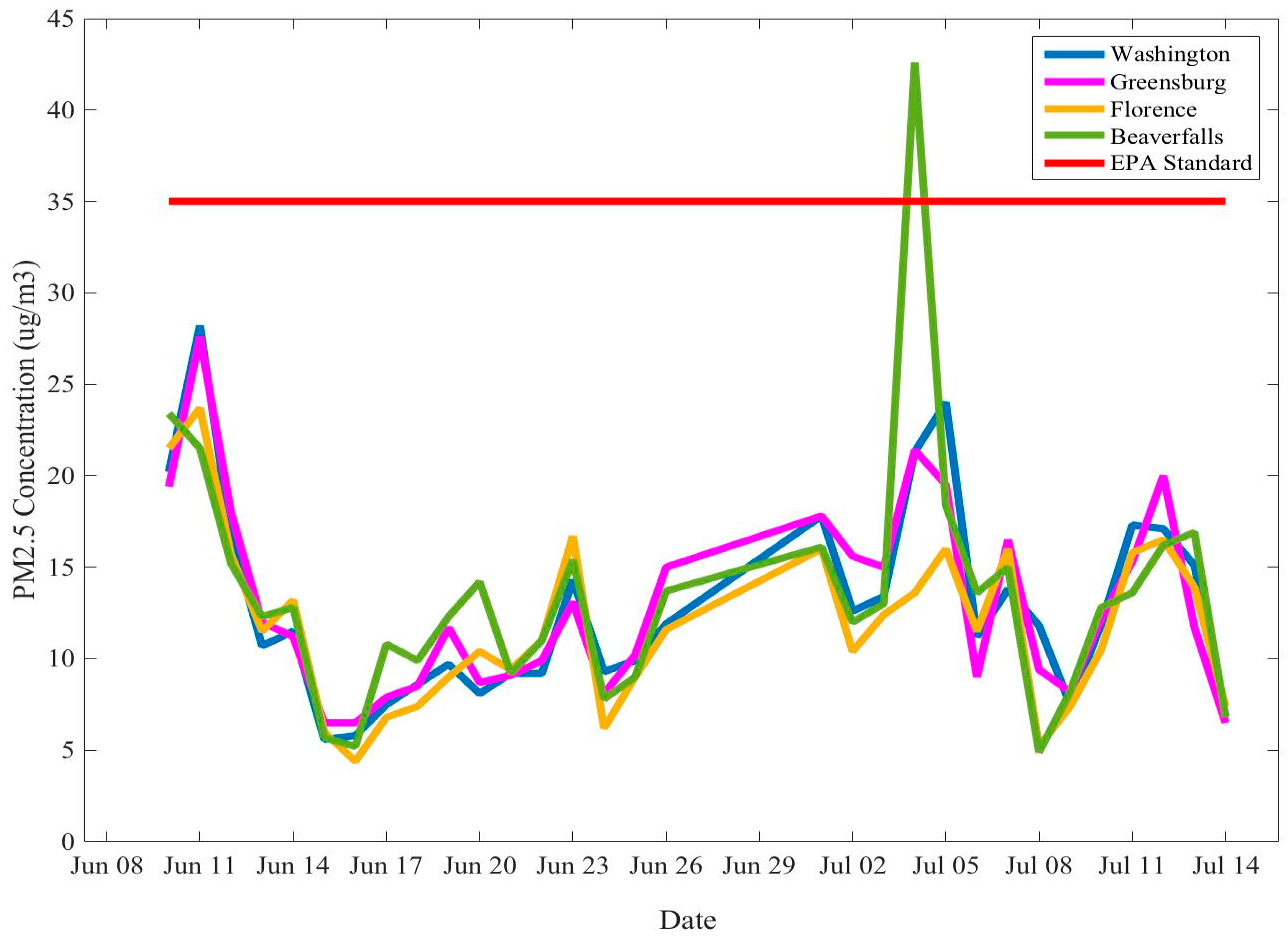
The concentrations of PM
2.5 measured by four PA Department of Environmental Protection air quality monitors were also analyzed in this study. The observed average 24-hour concentrations at these sites were 12.7 ± 6.9 μg m
−3 (Beaver Falls), 11.2 ± 4.7 μg m
−3 (Florence), 12.2 ± 5.3 μg m
−3 (Greensburg) and 12.2 ± 5.5 μg m
−3 (Washington). Similar to what was observed at the NCSU monitoring sites, the PA DEP monitors also observed 24-hour average concentrations of fine particulate (2–28.2 μg m
−3) matter below the US EPA 24-hour NAAQS (35 μg m
−3), with the exception of the Beaver Falls monitoring stations, which observed a concentration of 42.6 μg m
−3 on 4 July 2015 (
Figure 11). However, this elevated concentration can likely be explained by the presence of fireworks and other combustion processes due to the holiday.
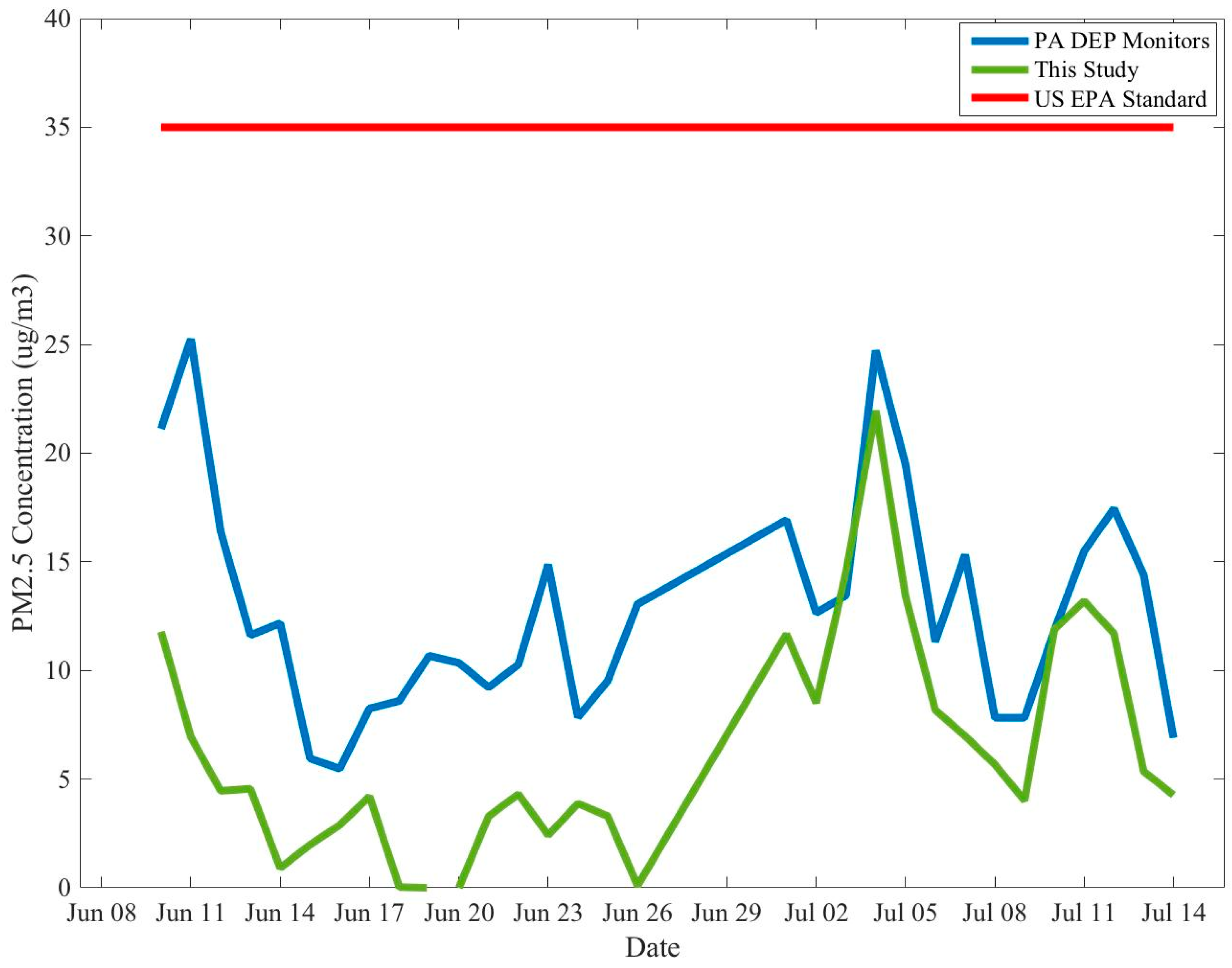
When comparing the average PA DEP monitoring station PM
2.5 concentrations [
20] with the average NCSU monitor PM
2.5 concentrations (
Figure 12), it is evident that the monitors used in this study observed lower concentrations than the concentrations observed at the PA DEP monitoring sites. However, the general trend in concentrations for both monitoring networks is the same. There are several possible explanations for this discrepancy. One potential cause for the differences in observations could be due to differences in the instrumentation used to measure the particulate matter. In addition, another potential cause for the observed differences could be due to location. Since the monitors are farther away, it is possible that the pollutants were transported aloft before mixing down to the surface level. Furthermore, it is also possible that there are other potential sources of particulate matter located near the sites.
4. Conclusions
The ambient 24-hour average concentrations of both PM2.5 (measured in this study as well as by the PA DEP) and PM10 did not reach levels higher than what is permitted by the US EPA 24-hour NAAQS. The average concentrations of PM10 observed during the periods were 20.5 ± 10.2 μg m−3 for Station 1, 16.1 ± 4.9 μg m−3 for Station 2 and 16.5 ± 7.1 μg m−3 for Station 3. The average concentrations of PM2.5 observed at the stations were 9.1 ± 5.1 μg m−3 for Station 1, 0.2 ± 0.4 μg m−3 for Station 2 and 11.6 ± 4.8 μg m−3 for Station 3. The highest average concentration was observed at Station 1 for PM10 and at Station 3 for PM2.5. However, Station 1 observed the highest daily average concentration for both PM2.5 and PM10. Not only was Station 1 the closest to the power plant, but the wind rose analysis showed that some of the elevated concentrations potentially came directly from the power plant’s coal pit, in addition to other PM sources. However, other elevated concentrations were observed coming from other directions, suggesting that there are several sources for particulate matter located in the region.
The IC analysis showed that the dominant species of particulate matter were primarily sulfate, nitrate and ammonium. The results of the XRF analysis showed that the primary constituents of PM10 and PM2.5 were sulfur, silicon, aluminum and iron. While these are all constituents that are observed from coal combustion emissions, these constituents are also prominent in most particulate matter speciation and therefore cannot be contributed directly to emissions from the Cheswick Power Plant.
The low particulate matter emissions and results of the speciation analyses could be attributed to a number of factors. Because the study period was so short, it is likely that the local scale meteorological conditions led to bias in the results. In addition, it is also possible that there were errors in the instrumentation that led to such low concentrations, particularly for PM
2.5 concentrations observed at Station 2. Furthermore, the low concentrations of particulate matter observed at the sites could also be attributed to the emission control technology that is added to the Cheswick power plant, which includes wet lime flue gas desulfurization, low NO
x burner technology with separated over fire air selective catalytic reduction and an electrostatic precipitator (Available online:
http://www.ampd.epa.gov/ampd), which would explain the reduced concentrations of pollutants observed in this study.
Based on the results of this study, is not possible to determine a concrete conclusion on the role of the Cheswick Power Plant in concentrations of particulate matter in the Cheswick and Springdale boroughs. These inconclusive results can be attributed to a number of factors, including unfavorable meteorological conditions, potential issues with the measurement equipment as well as an extremely short sampling period. It must be emphasized that this study was conducted over a limited time period. Therefore, it is recommended that further work be done on this matter, with longer sampling periods occurring in each season in order to capture a seasonal profile of concentrations of particulate matter in this region.


