Assimilating Conventional and Doppler Radar Data with a Hybrid Approach to Improve Forecasting of a Convective System


1
Collaborative Innovation Center on Forecast and Evaluation of Meteorological Disasters, Nanjing University of Information Science & Technology, Nanjing 210044, China
2
Key Laboratory of Meteorological Disaster of Ministry of Education, Nanjing University of Information Science & Technology, Nanjing 210044, China
3
Department of Atmospheric Science, Nanjing University of Information Science & Technology, Nanjing 210044, China
*
Author to whom correspondence should be addressed.
Atmosphere 2017, 8(10), 188; https://doi.org/10.3390/atmos8100188
Submission received: 18 August 2017
/
Revised: 22 September 2017
/
Accepted: 22 September 2017
/
Published: 25 September 2017
(This article belongs to the Section Meteorology)
Abstract
:A hybrid ensemble adjustment Kalman filter—three-dimensional ensemble—variational (EAKF-En3DVar) system is developed to assimilate conventional and radar data, and is applied to a convective case in Colorado and Kansas, USA. The system is based on the framework of the Weather Research and Forecasting model’s three-dimensional variational (3DVar) and Data Assimilation Research Testbed. A two-step assimilation procedure with a shorter length scale and analysis cycle is used to reduce analysis noise in radar data assimilation. Results show that the hybrid experiment assimilating only conventional data improves the quantitative precipitation forecast (QPF) and quantitative reflectivity forecast over those of a 3DVar experiment, and the improvements are also evident after assimilating radar data. The assimilation of radar data substantially improves the QPF up to seven hours, with either the 3DVar or hybrid method. The hybrid experiment assimilating both conventional and radar data forecasts a more accurate convective system in terms of structure, spatial extent and intensity and produces increased low-level cooling and mid-level warming in the convective region. These improvements are attributable to an improved forecast background field of wind, temperature and water vapor mixing ratio, with maximum root mean square error reduction at the tropopause and near the surface.
1. Introduction
Three-dimensional variational (3DVar) data assimilation (DA) has been a widely used technique in operational centers and the research communities. The Weather Research and Forecasting Data Assimilation (WRFDA) 3DVar system was originally developed for assimilating conventional large-scale observations and currently has the ability to assimilate observational data from multiple platforms [1,2]. Xiao et al. [3] demonstrated its capability to assimilate radar data by taking total water mixing ratio as a control variable for convective-scale assimilation. However, it is limited to warm rain microphysical schemes. Gao and Stensrud [4] developed another radar reflectivity forward operator that included an ice microphysical scheme using temperature-based hydrometeor classification to distinguish liquid water, snow and hail. A positive impact was found in the precipitation distribution and temperature field. Wang et al. [5] proposed an indirect approach for the WRFDA 3DVar radar DA system in which a procedure for assimilating in-cloud humidity estimated from radar reflectivity observations was added. The results showed that the new updating system substantially improved short-term precipitation prediction for convective events. However, static and climatological background error covariance (BEC) is used in the WRFDA 3DVar system, which was mainly designed for large-scale systems.
The ensemble Kalman filter (EnKF) proposed by Evensen [6] has gained much popularity in recent years as a potential alternative to the variational DA system. The EnKF uses a Monte Carlo approach to dynamically evolve the BEC, and covariance and cross-covariance calculated from a group of ensemble forecasts allows state variables not directly observed to be solved. This is especially valuable for storm-scale DA. Snyder and Zhang [7] were the first to demonstrate its ability to initialize convective storms by assimilating simulated radar radial velocity. Subsequent studies [8,9,10,11] developed radar forward operators to incorporate both radial velocity and reflectivity, and included complex microphysics schemes. These studies showed encouraging results for initialization, especially wind, temperature, moisture and microphysical fields, and the results can be further improved by the assimilation of conventional data. However, the BEC of EnKF is severely rank-deficient because the ensemble size is much smaller than the degrees of freedom of typical numerical weather prediction model states. This issue is commonly addressed by using covariance localization and inflation techniques [12]. Unfortunately, localization appears to destroy balance that may be present in the true forecast error, and tuning the inflation parameter is expensive, especially for convective-scale DA.
Motivated by these studies, a hybrid algorithm that aims to combine the advantages of both variational and ensemble approaches was proposed by Hamill and Snyder [13]. In their hybrid method, the static BEC in 3DVar was replaced directly by the combination of static and ensemble-derived BEC. Lorenc [14] suggested that ensemble-based estimates of covariance can be incorporated into the variational framework by using an extended variable, which is more easily implemented in different variational DA systems. This method was proven by Wang et al. [15] to be theoretically equivalent to the hybrid method proposed by Hamill and Snyder [13]. Wang et al. [16,17] demonstrated the potential advantage of the hybrid method over the standalone variational and EnKF method with limited ensemble size. More recently, Pan et al. [18] established a hybrid EnSRF-En3DVar system for the Rapid Refresh forecasting system and reported its improvements. For storm-scale DA, Gao and Stensrud [19] developed the hybrid EnKF-En3DVar radar DA system within Advanced Regional Prediction System model for a simulated storm, which can considerably improve the performance of 3DVar.
In this paper, we develop a hybrid ensemble adjustment Kalman filter—three-dimensional ensemble—variational (EAKF-En3DVar) system for WRF to assimilate conventional and radar data for a convective case in eastern Colorado and Kansas, USA. The key feature of this system is the means for effectively assimilating large-scale conventional data with three-hourly and radar data with hourly update cycle in an operational configuration. We adopted the two-step assimilation method of Tong et al. [20], in which radar observations are assimilated in a second step that follows a first step assimilating conventional observations from the Global Telecommunications System (GTS). Analysis from the first step provides a background first guess for the radar DA. As shown by Tong et al. [20], this two-step procedure is able to reduce analysis noise in radar DA by using a shorter length scale and analysis cycle.
2. Experiments
2.1. WRFDA 3DVar System
The cost function of WRFDA 3DVar can be written as
where is the background term and and are observation terms associated with GTS and radar data. Those data were assimilated in two separate steps, as presented in the following section. The u-wind and v-wind were used as momentum control variables in the convective system instead of the stream function and velocity. The other control variables were temperature (T), pseudo relatively humidity (RH), and surface pressure (Ps).
The radar radial velocity assimilation followed the procedure in Xiao and Sun [21], while radar reflectivity DA followed the indirect DA of Wang et al. [5]. Wang et al. [5] showed that by adding rainwater mixing ratio and in-cloud water vapor (both estimated from reflectivity), the indirect DA can avoid the linearization error of the reflectivity-rainwater equation. We also extend this method by adding snow and grauple-hail terms to the cost function. The cost function of the indirect radar reflectivity can be written as
and
where represents the rainwater mixing ratio, snow mixing ratio and graupel-hail mixing ratio of the atmospheric state, are their observations retrieved from radar reflectivity, and and are their related observational variances and background error matrix, respectively. , and are the water vapor mixing ratios, their observations retrieved from radar reflectivity and observational variances, respectively. The hydrometeor mixing ratios are estimated from reflectivity using relationships presented in Gao and Stensrud [4].
2.2. DART-EAKF System
The general linear ensemble update equations in the EnKF can be formulated as
where is the model state vector, denotes the NWP model, and is the current analysis time. stands for the Kalman gain matrix, is the observation operator that projects state variables into observed quantities, and is the linearized version of . and are covariance matrices of the observation and background errors, respectively. Here, subscript denotes the ensemble member order from 1 to , where is the ensemble size. Superscripts , , and stand for background, analysis and observations, respectively, and the overbar represents an ensemble mean.
To avoid additional sampling errors in the ensemble, we used the EAKF [22] within the Data Assimilation Research Testbed (DART) utility, in which observations are not perturbed randomly. Equation (5) for EAKF can be rewritten as
where is the inflation factor and is an identity matrix. The prime symbol in the equations represents the perturbation of ensemble members.
2.3. Hybrid EAKF-En3DVar
Based on the notation for the hybrid method for DA [23], the cost function in EAKF-En3DVar can be updated as
where is the term associated with the ensemble BEC, and are the static and ensemble-derived BEC matrices, and is the observation operator. Here, is the analysis increment of the state vector, defined as
where is the analysis increment associated with the static BEC, is the kth ensemble background perturbation normalized by , where is the ensemble member size. Vectors represent the extended control variables, and subscript denotes scalar multiplication.
Two coefficients, and , define weights prescribed in the static and ensemble BEC, which satisfies the relationship
where is the weight of the static BEC matrix and is the weight of the ensemble-derived BEC matrix.
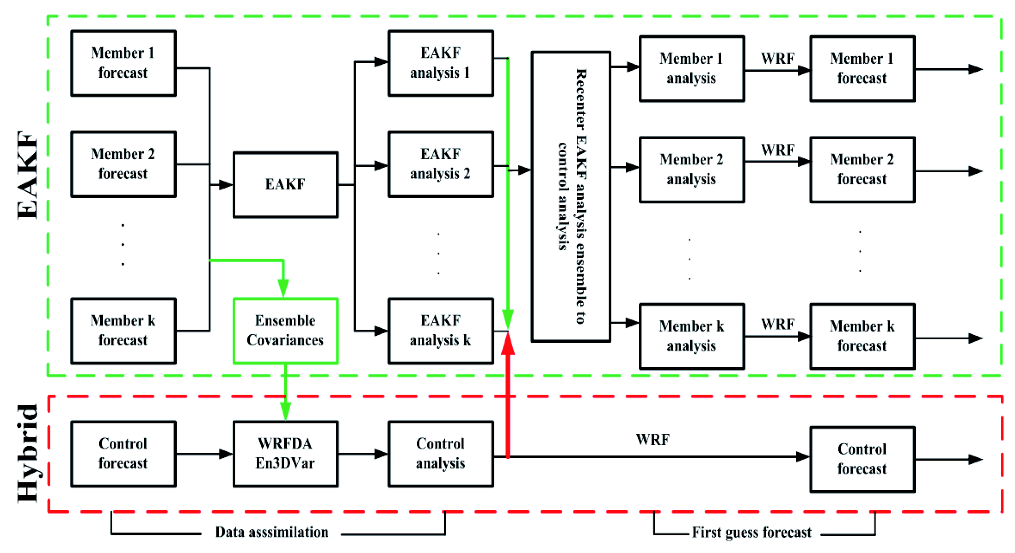
Figure 1 illustrates how the coupled hybrid EAKF-En3DVar system works. In the variational minimization, the flow-dependent BEC is incorporated into the 3DVar framework by extending the control variables. Then, the control forecast is updated using the hybrid method and the forecast ensemble perturbations updated by EAKF, in order to obtain the analysis ensemble perturbations. Finally, the EAKF analysis ensembles are recentered to the En3DVar control analysis.
2.4. Overview of Convective Case
The convective system formed under the influence of a cold front, and convergence between northerly cold-dry and southerly warm-moist air helped initiate convection in Colorado. The heaviest rainfall was in western Kansas, with a maximum of 55.4 mm in a one-hour period. Maximum wind speed exceeded 24.1 m s−1. Figure 2 shows composite radar reflectivity at four times, representing the evolution of the convective system in Colorado and Kansas on 7 August 2016. At 03:00 UTC (Figure 2a), two convective cells were developing, one in eastern Kansas and the other around the Oklahoma panhandle. At that time, another convective cell formed in Colorado. At 06:00 UTC (Figure 2b), these convective cells merged, strengthened and organized into a strong convective system with maximum reflectivity of 55 dBZ. At 10:00 UTC (Figure 2c), this system moved to Kansas and a convective line at its leading edge intensified, with broad stratiform precipitation behind. At 12:00 UTC (Figure 2d), the system weakened and the area of reflectivity >30 dBZ shrank.
2.5. Experiment Design and Verification Methods
We used WRF version 3.9 in the present study. The model was configured with two domains, inner and outer, with horizontal resolutions of 15 and 3 km, respectively. There were 51 vertical levels and a model top at 50 hPa. The model domains and radar station locations are shown in Figure 3. The Kain-Fritsch cumulus parameterization scheme [24] was only used in Domain 1. Other model physics schemes were the Thompson microphysics scheme [25], Mellor–Yamada–Janjić planetary boundary layer model [26], Noah land surface model [27], Rapid Radiative Transfer Model for GCMs (RRTMG) longwave radiation, and RRTMG shortwave radiation [28].
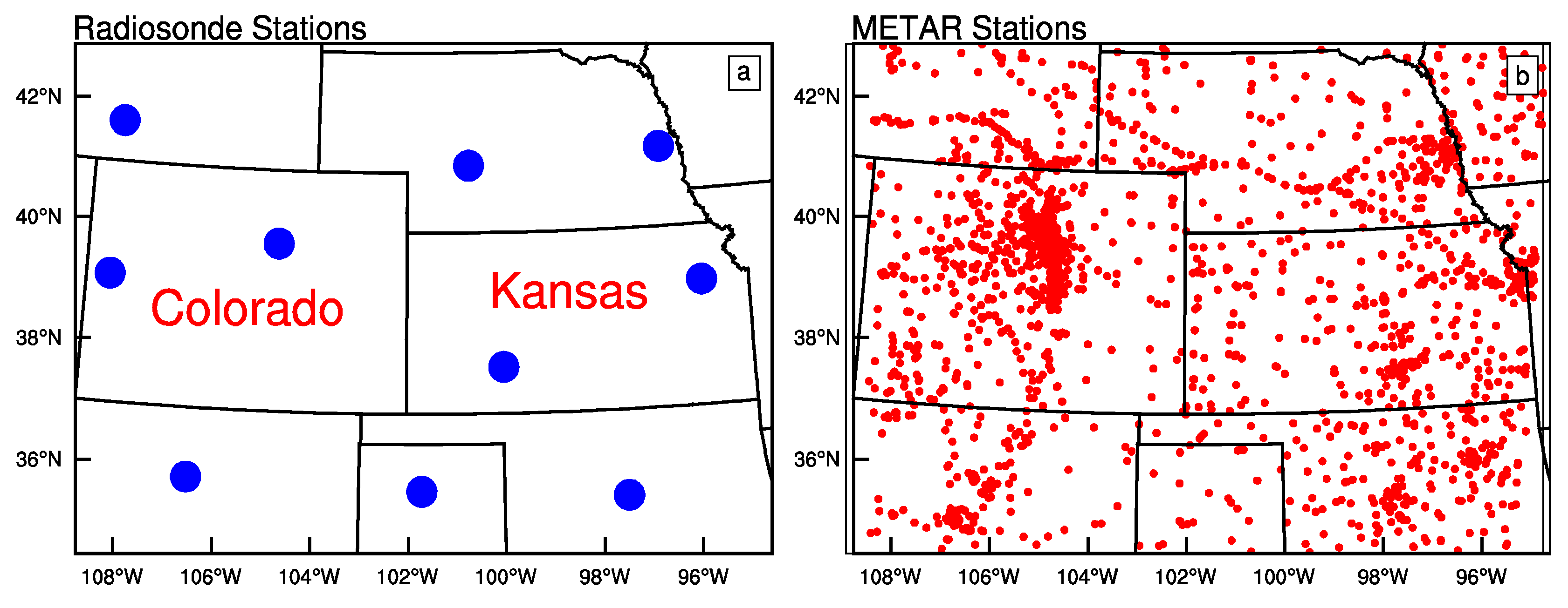
Data from 17 radar stations were used, as shown in Figure 3. Radar data were preprocessed using a quality control procedure in the Variational Doppler Radar Assimilation System [29]. Quantitative precipitation estimates from the Multi-Radar/Multi-Sensor System [30] were used as observations for precipitation verification. In addition, verification against radiosondes and METAR observations (see Figure 4) were also performed for all experiments.
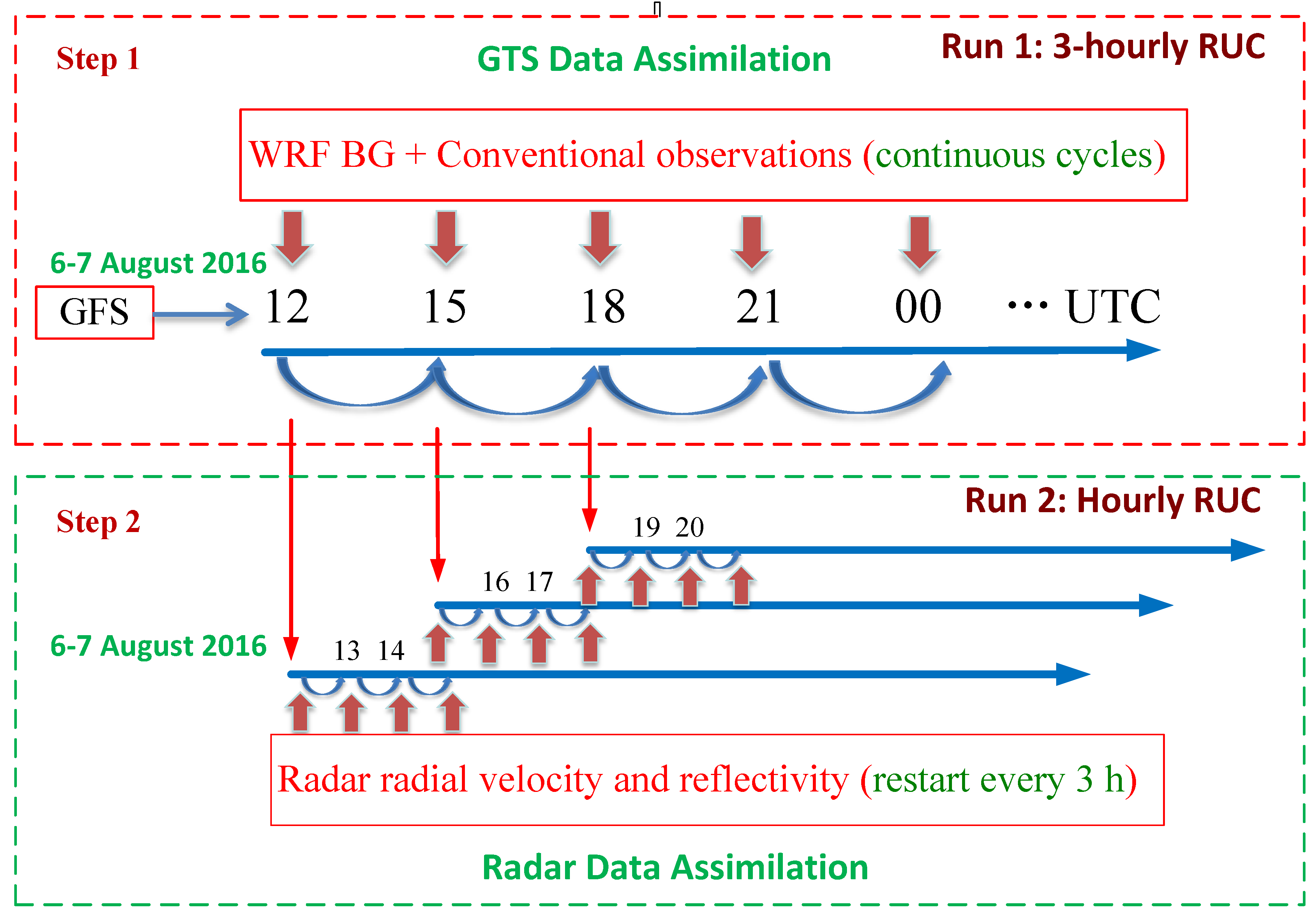
The radar DA experiments followed the two-step procedure of Tong et al. (2016), as shown in Figure 5. In Step 1, the first assimilation cycle was initiated at 12:00 UTC on 6 August 2016 with GTS, with radiosonde, surface network and aircraft data assimilated. Then, three-hourly analysis/forecast cycles were executed through 09:00 UTC on 7 August 2016. The analysis following GTS assimilation was used as background for the radar DA in Step 2, every third hour (12:00, 15:00, 18:00, etc. UTC). Then, 0–12 h forecasts were made beginning at 15:00, 18:00, 21:00, 00:00, 03:00, 06:00 and 09:00 UTC, after the three-hourly cycles of radar DA.
A description of these experiments is in Table 1. Exp3DVC and ExpHYBC refer to experiments only assimilating GTS using the 3DVar and hybrid methods, respectively. Exp3DVCR and ExpHYBCR refer to experiments assimilating both GTS and radar data with the two-step assimilation scheme. For the Exp3DVCR, the analysis is produced by assimilating GTS data in Step 1 as background (3DVar_GTS). Then, the radar observations are assimilated to produce another 3DVar analysis using 3DVar_GTS as background in Step 2. For the ExpHYBCR, in Step 1, GTS data are continuously assimilated to generate En3DVar analysis (En3DVar_GTS). Meanwhile, EAKF also continuously assimilates GTS data to update forecast ensemble to analysis ensemble (EAKF_GTS). In Step 2, the radar observations are assimilated to produce another En3DVar analysis (En3DVar_Radar), using En3DVar_GTS as the background. The EAKF also assimilates radar data (EAKF_Radar) using the analysis members (EAKF_GTS) as background from the Step 1.
Each hybrid experiment (ExpHYBC and ExpHYBCR) assigned equal weight (50%) to the static and ensemble BEC. Forty members were created using the method of “random CV” described in Baker [31]. The horizontal covariance localization radius was 60 km for Domain 1 and 20 km for Domain 2, and the vertical covariance localization radius was 4 km for the two domains. We used a Bayesian inflation method [32] that varied adaptively in both space and time.
To quantitatively assess quantitative precipitation and reflectivity forecast performance, the fractions skill score (FSS) proposed by Roberts and Lean [33] was used to verify forecast skill of precipitation and reflectivity. The FSS is defined as:
where and denote forecast and observed fractions of each grid when the forecast or observation is larger than a given threshold value, and is the number of grid points where the observation exceeds the threshold. FSS range is 0–1 and larger values indicate greater prediction skill. In our study, the FSS was calculated for each forecast time and grid using neighborhood sizes of 10 km. It was then averaged over the domain every hour. Two other forecast error statistics, the equitable threat score (ETS) and Probability of Detection (POD) [34], were also calculated:
where , and represent hits, false alarms and misses. is hits expected from random chance, and is the total number of hits, false alarms, misses and grid points where the observed and forecast are both less than the threshold. We also did verification against radiosondes and surface observations using root mean square errors (RMSEs) of wind, temperature, and humidity.
3. Results
3.1. Comparison of Precipitation
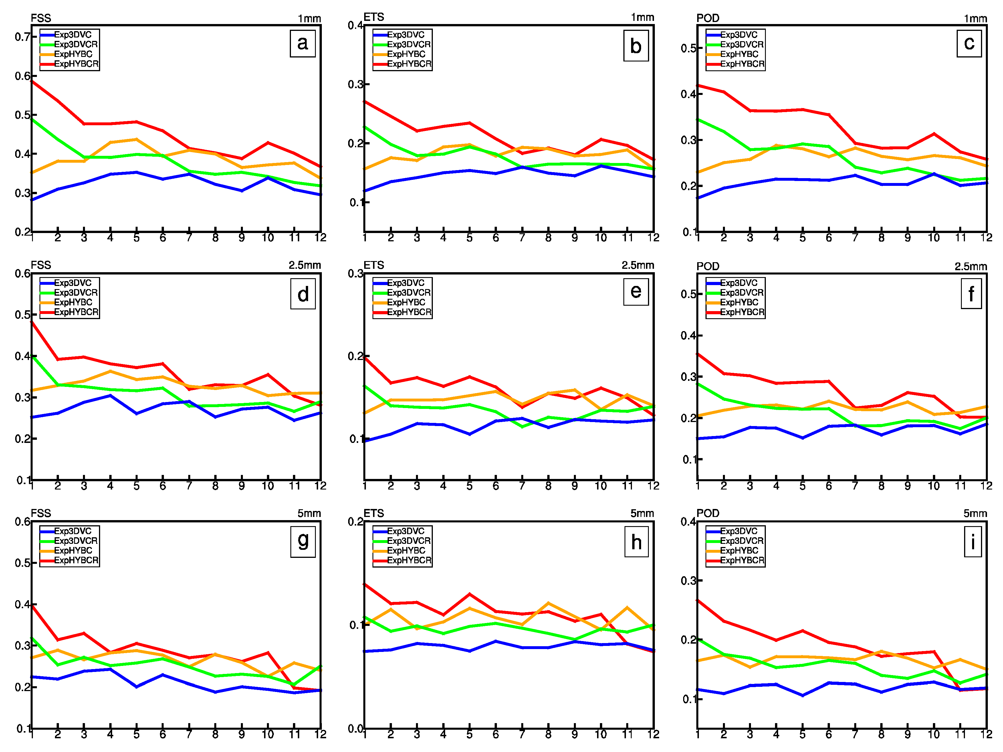
The results of FSS, ETS and POD (see the panels by column) from Exp3DVC, ExpHYBC, Exp3DVCR and ExpHYBCR (Table 1) for hourly accumulated precipitation are compared in Figure 6 for thresholds 1, 2.5 and 5 mm (see the panels by line), respectively. The skill scores were computed for seven forecasts initialized at 15:00, 18:00, 21:00, 00:00, 03:00, 06:00 and 09:00 UTC averaged in Domain 2. It is clear that ExpHYBCR (red curve) has the highest FSS for all thresholds during the first seven hours. The ExpHYBCR has higher FSS than Exp3DVCR (green curve) and ExpHYBC (orange curve) has higher FSS than Exp3DVC (blue curve), suggesting the effectiveness of the hybrid method. The FSS of Exp3DVCR is higher than Exp3DVC for all precipitation thresholds, and the differences are the largest in the first four hours. This is also true for ExpHYBCR and ExpHYBC. Between seven and nine hours, the FSS of ExpHYBCR and ExpHYBC for all thresholds are comparable, and the differences between Exp3DVCR and Exp3DVC are smallest at seven hours for thresholds 1 and 2.5 mm. This suggests that the assimilation of radar data can improve the short-term precipitation forecast out to seven hours, consistent with the conclusion of Wang et al. [5]. The FSS of Exp3DVC is the poorest throughout the entire forecast and never exceeds 0.4. These features are confirmed by ETS and POD.
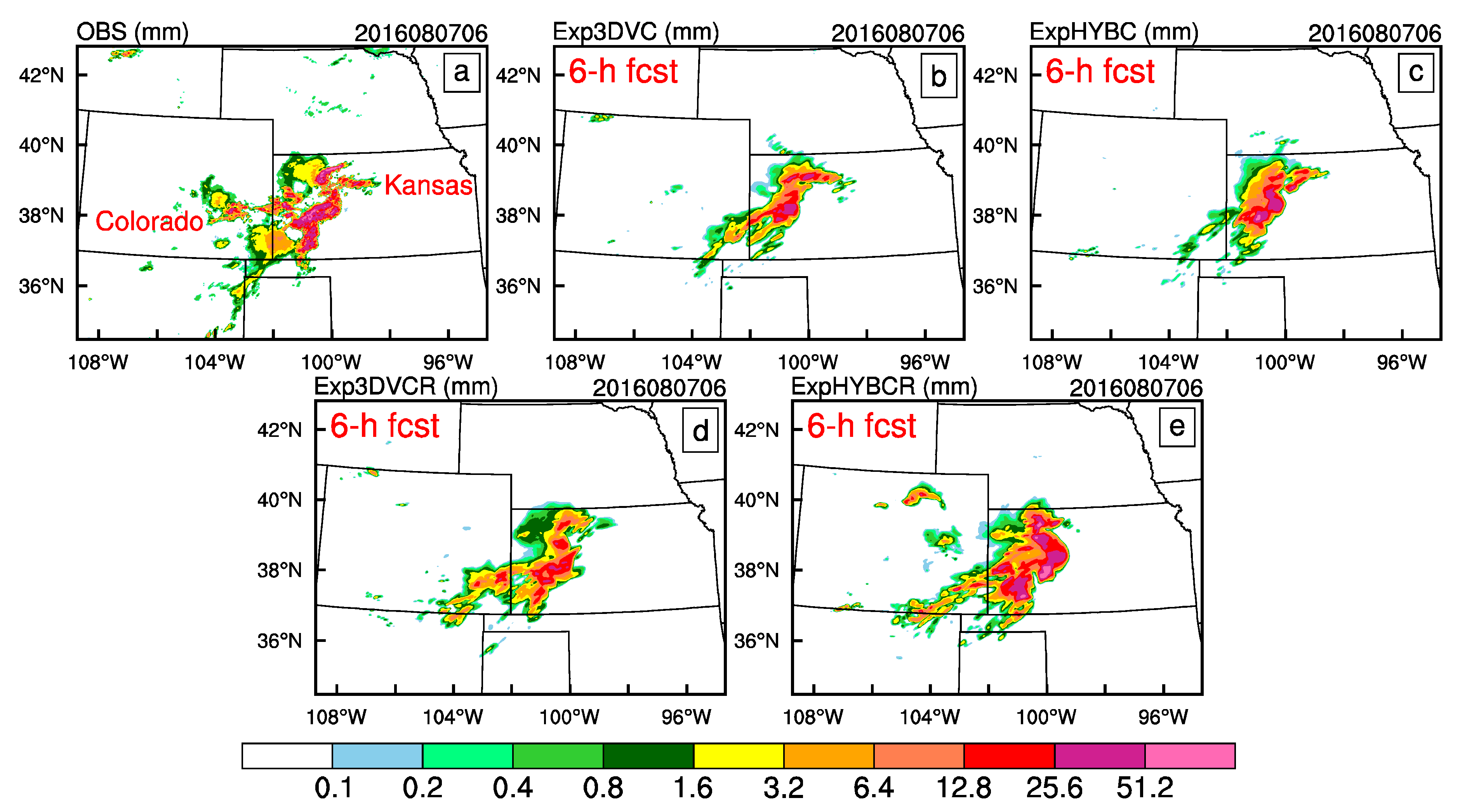
Figure 7 shows a comparison of hourly accumulated precipitation between observation, Exp3DVC, ExpHYBC, Exp3DVCR and ExpHYBCR at 05:00 UTC on 7 August 2016, from 5-h forecasts initialized at 00:00 UTC on 7 August 2016. Figure 7a shows some disorganized rainfall, and two heavy rainfall areas are found in western Kansas with maximum rainfall amount of ~55 mm. Exp3DVC (Figure 7b) underestimated the heavy rainfall amount, whereas ExpHYBC (Figure 7c) shows closer strength with observation over the above areas. The experiment with radar DA, Exp3DVCR and ExpHYBCR (Figure 7d,e) all show some improvements over corresponding experiments without radar DA by producing more rainfall in southwestern Kansas. In ExpHYBCR, the area of the precipitation >25 mm is very similar to the shape of the observations. By 06:00 UTC (Figure 8), some weak rainfall had moved east and developed into a large and strong rainbelt (>25 mm) in Kansas. Again, the rainfall pattern and amounts in the rain-belt region was better captured by ExpHYBC (Figure 8c) as compared to Exp3DVC (Figure 8b). However, the southern part of the rainbelt is absent. The radar DA experiments, especially ExpHYBCR (Figure 8e), improved the forecast precipitation pattern in southwestern Kansas, and some separated weaker precipitation over eastern Colorado was successfully predicted.
Figure 9 shows a comparison of hourly accumulated precipitation between observation, Exp3DVC, ExpHYBC, Exp3DVCR and ExpHYBCR at 07:00 UTC on 7 August 2016, from 4-h forecasts initialized at 03:00 UTC on 7 August 2016. Exp3DVC (Figure 9b) still underestimated the rainfall amount and failed to simulate the shape of the heavy rainfall center. The heavy rainfall pattern of ExpHYBC (Figure 9c) was relatively well simulated compared to Exp3DVC, but rainfall between 1.6 mm and 6.4 mm at the Kansas–Colorado border was poorly simulated. These misrepresentations were reduced in Exp3DVCR and ExpHYBCR (Figure 9d,e), and the best result was from ExpHYBCR. Particularly encouraging is that the main heavy rainfall center in ExpHYBCR agreed especially well with observations in terms of shape and intensity. At 09:00 UTC (Figure 10), the heavy rainfall center remained pronounced and well-organized, and its northern part moved faster than its southern part. Comparison of Exp3DVC and Exp3DVCR shows a similar pattern (Figure 10b,d), but Exp3DVCR had a heavier rainfall center that was more similar to observation. This was also true for ExpHYBC and ExpHYBCR (Figure 10c,e). When compared to the experiments using different assimilation methods, the northern part of the convective line in Exp3DVC and Exp3DVCR was displaced to the east, with improvement in the hybrid experiments. In addition, ExpHYBCR successful predicted the shape of the heavy rainfall, though with some overestimation.
3.2. Comparison of Reflectivity
There were also substantially different features of simulated reflectivity from the four experiments. Figure 11 shows FSS, ETS and POD for those experiments (see the panels by column), using thresholds of 5, 15 and 25 dBZ, respectively (see the panels by line). ExpHYBCR (red curve) retained a very high FSS for all thresholds, and its scores are as much as 0.25 greater than those of EXP3DVC (blue curve) in the first three hours. The hybrid experiments show higher FSS than those of corresponding 3DVar experiments, and the FSS of Exp3DVCR (green curve) was not always higher than those of EXPHYBC (orange curve). The same comparison holds for ETS and POD for all thresholds. However, with the assimilation of radar data in either 3DVar or hybrid experiments, reflectivity scores generally increased, and differences were relatively large in the first three hours.
Differences of the four experiments were pronounced at 06:00 UTC (6-h forecast initialized at 00:00 UTC) and 07:00 UTC (4-h forecast initialized at 03:00 UTC) on 7 August 2016. At 06:00 UTC (Figure 12), convective cells strengthened and organized into two convective lines and broad stratiform precipitation areas. Compared with observation, ExpHYBC (Figure 12c) was better than Exp3DVC (Figure 12b) in representing the convective system, with a longer convective line and more stratiform precipitation. With further radar DA, the simulated convective system in Exp3DVCR and ExpHYBCR (Figure 12d,e) strengthened and better matched the observation. ExpHYBCR successfully predicted the shape and intensity of the convective line and broader stratiform precipitation, comparing reasonably well with observation. These features in the four experiments persisted until 07:00 UTC (Figure 13) and ExpHYBCR (Figure 13e) again gave the best result, with better representation of the convective line and stratiform precipitation. When compared with the experiment without radar DA, Exp3DVCR and ExpHYBCR (Figure 13d,e) also predicted some convective activity near Colorado, as observed.
3.3. Average RMSE of Forecast Background
The differences in forecast precipitation and reflectivity of the four experiments can be attributed to differences in the background. Figure 14 shows average RMSEs of horizontal wind components, temperature, and water vapor forecast background against all 10 radiosondes in the 3-km domain shown in Figure 4a. In particular, RMSEs of ExpHYBC (orange curve) were generally slightly less than those of Exp3DVC (blue curve). Such improvements of ExpHYBCR (red curve) over Exp3DVCR (green curve) were also found at the tropopause. There is a large reduction for the ExpHYBCR (Exp3DVCR) compared to ExpHYBC (Exp3DVC), and differences are more evident for winds below 150 hPa. This indicates that the inclusion of additional radar DA can improve the forecast background. Further, the improvement of ExpHYBCR over ExpHYBC is greater than that of ExpHYBCR over Exp3DVCR. Figure 15 shows average RMSEs of horizontal wind components, temperature, and water vapor analyses against all surface METAR stations in the 3-km domain showed in Figure 4b. It is seen that ExpHYBCR (red bar) had the smallest RMSE for u, v, T and Q, followed by ExpHYBC and Exp3DVCR (orange and green bar, respectively). Again, both the 3DVAR and hybrid experiments generally had smaller RMSEs when radar data were assimilated.
3.4. Temperature and Wind Fields
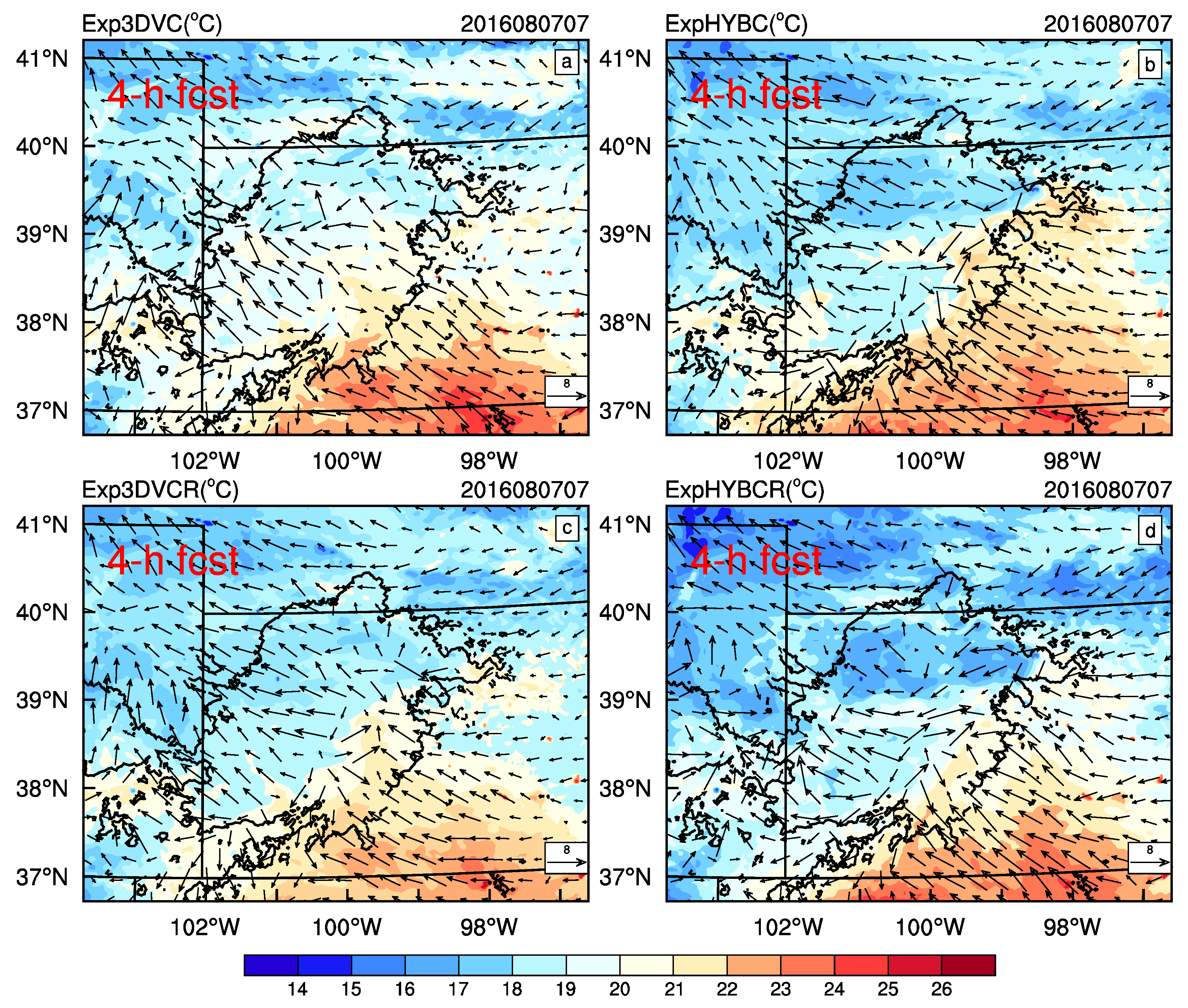
Figure 16 and Figure 17 show temperature and horizontal wind fields at different levels of Exp3DVC, ExpHYBC, Exp3DVCR and ExpHYBCR at 07:00 UTC on 7 August 2016. Solid black lines represent contours of observed reflectivity > 20 dBZ. At the surface (Figure 16), ExpHYBCR (Figure 16d) produced a large cold pool with minimum temperatures 15–17 °C around northern Kansas, which was likely caused by strong evaporative cooling corresponding to increased precipitation from using the hybrid method and assimilation of radar data. When rain drops into unsaturated air, they evaporate and eventually lead to a descent of cold pool near the surface. Temperatures of Exp3DVC, ExpHYBC and Exp3DVCR (Figure 16a–c) in the same region were about 18–19 °C, 16–18 °C and 17–19 °C, respectively. There was much stronger wind in southern Kansas from ExpHYBCR compared to the other experiments, which supports a stronger cold pool.
At 500 hPa (Figure 17), ExpHYBCR (Figure 17d) shows the largest warm area, with maximum temperature −1 °C. This is because of the strong condensation heating at mid-levels, which is closely related to the formation and development of mesoscale convective system (MCS). Compared with Exp3DVC, ExpHYBC and Exp3DVCR (Figure 17a–c) generated a larger area of temperature > −3.5 °C.
4. Discussion and Conclusions
In this study, we applied a coupled hybrid EAKF-En3DVar system developed for WRF to assimilate conventional and radar observations to a convective system in Colorado and Kansas. The indirect radar DA approach of Wang et al. (2013) was used for radar reflectivity, in which retrieved hydrometer mixing ratios were assimilated. The two-step procedure of Tong et al. (2016) was also used to reduce analysis noise in radar DA, via the use of a shorter length scale and analysis cycle. The system was examined by comparing experimental forecast results, i.e., using 3DVar and hybrid experiments without (Exp3DVC and ExpHYBC) and with radar DA (Exp3DVCR and ExpHYBCR). The Exp3DVCR and ExpHYBCR refer to the experiments assimilating GTS data and radar data with the two-step procedure.
The results show that ExpHYBC improved quantitative precipitation forecasts relative to Exp3DVC, and such improvements were also evident from assimilating radar data for thresholds of 1, 2.5 and 5 mm as measured by FSS, ETS and POD. In general, the assimilation of radar data in either 3DVar or hybrid experiments could considerably improve short-term precipitation forecasts up to seven hours.
The hybrid experiments more accurately reproduced observed rainfall amounts than the experiments using 3DVar, especially regarding the structure and intensity of the heavy rainfall center. By assimilating radar data, convective precipitation over southwestern Kansas and some isolated precipitation were better captured than with Exp3DVC and ExpHYBC. Overall, ExpHYBCR produced the strongest resemblance with observations in terms of spatial extent, intensity, and shape. We reached a similar conclusion for reflectivity forecasts. That was based on improved quantitative reflectivity forecasts and superior representation of convective line and stratiform precipitation structure and intensity from use of the hybrid method and radar data assimilation.
The improved precipitation and reflectivity skill is attributable to improvements in the forecast background field of wind, temperature, and water vapor mixing ratio, as verified against radiosondes in the 3-km domain. Radar DA with the hybrid method enhanced low-level cooling because of rainwater evaporation and mid-level warming associated with latent heating, in addition to stronger winds in the convective region.
Despite such encouraging results for the hybrid EAKF-En3DVar system, more convective cases are needed for future study. Work is still needed to further improve the hybrid system using more advanced variational methods, such as 4DEnVar.
Acknowledgments
This research was supported by Research Innovation Program for College Graduates of Jiangsu Province (Grant Nos. KYLX_0829 and KYLX_0844). The authors Shibo Gao and Danlian Huang are supported by scholarships from the China Scholarship Council.
Author Contributions
Shibo Gao designed, performed the experiments and wrote the paper. Danlian Huang provided scientific insight, and wrote and edited the manuscript.
Conflicts of Interest
The authors declare no conflict of interest.
References
- Barker, D.M.; Huang, W.; Guo, Y.-R.; Bourgeois, A.J.; Xiao, Q. A Three-Dimensional Variational Data Assimilation System for MM5: Implementation and Initial Results. Mon. Weather Rev. 2004, 132, 897–914. [Google Scholar] [CrossRef]
- Barker, D.; Huang, X.Y.; Liu, Z.; Auligné, T.; Zhang, X.; Rugg, S.; Ajjaji, R.; Bourgeois, A.; Bray, J.; Chen, Y.; Demirtas, M.; Guo, Y.-R.; Henderson, T.; Huang, W.; Lin, H.C.; Michalakes, J.; Rizvi, S.; Zhang, X. The weather research and forecasting model’s community variational/ensemble data assimilation system: WRFDA. Bull. Am. Meteorol. Soc. 2012, 93, 831–843. [Google Scholar] [CrossRef]
- Xiao, Q.; Kuo, Y.H.; Sun, J.; Lee, W.C.; Barker, D.M.; Lim, E. An approach of radar reflectivity data assimilation and its assessment with the Inland QPE of Typhoon Rusa (2002) at landfall. J. Appl. Meteorol. Climatol. 2007, 46, 14–22. [Google Scholar] [CrossRef]
- Gao, J.; Stensrud, D.J. Assimilation of Reflectivity Data in a Convective-Scale, Cycled 3DVAR Framework with Hydrometeor Classification. J. Atmos. Sci. 2012, 69, 1054–1065. [Google Scholar] [CrossRef]
- Wang, H.; Sun, J.; Fan, S.; Huang, X.Y. Indirect assimilation of radar reflectivity with WRF 3D-Var and its impact on prediction of four summertime convective events. J. Appl. Meteorol. Climatol. 2013, 52, 889–902. [Google Scholar] [CrossRef]
- Evensen, G. Sequential data assimilation with a nonlinear quasi-geostrophic model using Monte Carlo methods to forecast error statistics. J. Geophys. Res. 1994, 99, 10143–10162. [Google Scholar] [CrossRef]
- Snyder, C.; Zhang, F. Assimilation of Simulated Doppler Radar Observations with an Ensemble Kalman Filter. Mon. Weather Rev. 2003, 131, 1663–1677. [Google Scholar] [CrossRef]
- Tong, M.; Xue, M. Ensemble Kalman filter assimilation of Doppler radar data with a compressible nonhydrostatic model: OSSE experiments. Mon. Weather Rev. 2005, 133, 1789–1807. [Google Scholar] [CrossRef]
- Xue, M.; Tong, M.; Droegemeier, K.K. An OSSE framework based on the ensemble square root Kalman filter for evaluating the impact of data from radar networks on thunderstorm analysis and forecasting. J. Atmos. Ocean. Tech. 2006, 23, 46–66. [Google Scholar] [CrossRef]
- Jung, Y.; Xue, M.; Tong, M. Ensemble Kalman Filter Analyses of the 29–30 May 2004 Oklahoma Tornadic Thunderstorm Using One- and Two-Moment Bulk Microphysics Schemes, with Verification against Polarimetric Radar Data. Mon. Weather Rev. 2012, 140, 1457–1475. [Google Scholar] [CrossRef]
- Putnam, B.J.; Xue, M.; Jung, Y.; Snook, N.; Zhang, G. The Analysis and Prediction of Microphysical States and Polarimetric Radar Variables in a Mesoscale Convective System Using Double-Moment Microphysics, Multinetwork Radar Data, and the Ensemble Kalman Filter. Mon. Weather Rev. 2014, 142, 141–162. [Google Scholar] [CrossRef]
- Anderson, J.L. Localization and Sampling Error Correction in Ensemble Kalman Filter Data Assimilation. Mon. Weather Rev. 2012, 140, 2359–2371. [Google Scholar] [CrossRef]
- Hamill, T.M.; Snyder, C. A Hybrid Ensemble Kalman Filter–3D Variational Analysis Scheme. Mon. Weather Rev. 2000, 128, 2905–2919. [Google Scholar] [CrossRef]
- Lorenc, A.C. The potential of the ensemble Kalman filter for NWP—a comparison with 4D-Var. Q. J. R. Meteorol. Soc. 2003, 129, 3183–3203. [Google Scholar] [CrossRef]
- Wang, X.; Snyder, C.; Hamill, T.M. On the Theoretical Equivalence of Differently Proposed Ensemble–3DVAR Hybrid Analysis Schemes. Mon. Weather Rev. 2007, 135, 222–227. [Google Scholar] [CrossRef]
- Wang, X.; Barker, D.M.; Snyder, C.; Hamill, T.M. A Hybrid ETKF–3DVAR Data Assimilation Scheme for the WRF Model. Part I: Observing System Simulation Experiment. Mon. Weather Rev. 2008, 136, 5116–5131. [Google Scholar] [CrossRef]
- Wang, X.; Barker, D.M.; Snyder, C.; Hamill, T.M. A Hybrid ETKF–3DVAR Data Assimilation Scheme for the WRF Model. Part II: Real Observation Experiments. Mon. Weather Rev. 2008, 136, 5132–5147. [Google Scholar] [CrossRef]
- Pan, Y.; Zhu, K.; Xue, M.; Wang, X.; Hu, M.; Benjamin, S.G.; Weygandt, S.S.; Whitaker, J.S. A GSI-Based Coupled EnSRF–En3DVar Hybrid Data Assimilation System for the Operational Rapid Refresh Model: Tests at a Reduced Resolution. Mon. Weather Rev. 2014, 142, 3756–3780. [Google Scholar] [CrossRef]
- Gao, J.; Stensrud, D.J. Some Observing System Simulation Experiments with a Hybrid 3DEnVAR System for Storm-Scale Radar Data Assimilation. Mon. Weather Rev. 2014, 142, 3326–3346. [Google Scholar] [CrossRef]
- Tong, W.; Li, G.; Sun, J.; Tang, X.; Zhang, Y. Design Strategies of an Hourly Update 3DVAR Data Assimilation System for Improved Convective Forecasting. Weather Forecast. 2016, 31, 1673–1695. [Google Scholar] [CrossRef]
- Xiao, Q.; Sun, J. Multiple-Radar Data Assimilation and Short-Range Quantitative Precipitation Forecasting of a Squall Line Observed during IHOP_2002. Mon. Weather Rev. 2007, 135, 3381–3404. [Google Scholar] [CrossRef]
- Anderson, J.L. An Ensemble Adjustment Kalman Filter for Data Assimilation. Mon. Weather Rev. 2001, 129, 2884–2903. [Google Scholar] [CrossRef]
- Wang, X. Incorporating Ensemble Covariance in the Gridpoint Statistical Interpolation Variational Minimization: A Mathematical Framework. Mon. Weather Rev. 2010, 138, 2990–2995. [Google Scholar] [CrossRef]
- Kain, J.S.; Fritsch, J.M. A One-Dimensional Entraining/Detraining Plume Model and Its Application in Convective Parameterization. J. Atmos. Sci. 1990, 47, 2784–2802. [Google Scholar] [CrossRef]
- Thompson, G.; Rasmussen, R.M.; Manning, K. Explicit Forecasts of Winter Precipitation Using an Improved Bulk Microphysics Scheme. Part I: Description and Sensitivity Analysis. Mon. Weather Rev. 2004, 132, 519–542. [Google Scholar] [CrossRef]
- Janjić, Z.I. The Step-Mountain Eta Coordinate Model: Further Developments of the Convection, Viscous Sublayer, and Turbulence Closure Schemes. Mon. Weather Rev. 1994, 122, 927–945. [Google Scholar] [CrossRef]
- Chen, F.; Dudhia, J. Coupling an Advanced Land Surface–Hydrology Model with the Penn State–NCAR MM5 Modeling System. Part I: Model Implementation and Sensitivity. Mon. Weather Rev. 2001, 129, 569–585. [Google Scholar] [CrossRef]
- Iacono, M.J.; Delamere, J.S.; Mlawer, E.J.; Shephard, M.W.; Clough, S.A.; Collins, W.D. Radiative forcing by long-lived greenhouse gases: Calculations with the AER radiative transfer models. J. Geophys. Res. Atmos. 2008, 113, D13103. [Google Scholar] [CrossRef]
- Sun, J. Initialization and Numerical Forecasting of a Supercell Storm Observed during STEPS. Mon. Weather Rev. 2005, 133, 793–813. [Google Scholar] [CrossRef]
- Zhang, J.; Howard, K.; Langston, C.; Kaney, B.; Qi, Y.; Tang, L.; Grams, H.; Wang, Y.; Cocks, S.; Martinaitis, S.; Arthur, A.; Cooper, K.; Brogden, J.; Kitzmillller, D. Multi-Radar Multi-Sensor (MRMS) quantitative precipitation estimation: Initial operating capabilities. Bull. Am. Meteorol. Soc. 2016, 97, 621–638. [Google Scholar] [CrossRef]
- Barker, D.M. Southern High-Latitude Ensemble Data Assimilation in the Antarctic Mesoscale Prediction System. Mon. Weather Rev. 2005, 133, 3431–3449. [Google Scholar] [CrossRef]
- Anderson, J.L. An adaptive covariance inflation error correction algorithm for ensemble filters. Tellus A 2007, 59, 210–224. [Google Scholar] [CrossRef]
- Roberts, N.M.; Lean, H.W. Scale-Selective Verification of Rainfall Accumulations from High-Resolution Forecasts of Convective Events. Mon. Weather Rev. 2008, 136, 78–97. [Google Scholar] [CrossRef]
- Mashingia, F.; Mtalo, F.; Bruen, M. Validation of remotely sensed rainfall over major climatic regions in Northeast Tanzania. Phys. Chem. Earth 2014, 67–69, 55–63. [Google Scholar] [CrossRef]
Figure 1.
Implementation and framework of a hybrid ensemble adjustment Kalman filter—three-dimensional ensemble—variational (EAKF-En3DVar) radar data assimilation system, with coupling between EAKF (green dashed box) and En3DVar (red dashed box) hybrid control analysis. The thick red arrow indicates the feedback of En3DVar hybrid control analysis to the EAKF, when the En3DVar hybrid control analysis is used to the replace the ensemble mean of the EAKF analyses.

Figure 2.
Observations of composite radar reflectivity (unit: dBZ) showing evolution of the convective system at: (a) 03:00 UTC; (b) 06:00 UTC; (c) 10:00 UTC; and (d) 12:00 UTC on 7 August 2016.
Figure 2.
Observations of composite radar reflectivity (unit: dBZ) showing evolution of the convective system at: (a) 03:00 UTC; (b) 06:00 UTC; (c) 10:00 UTC; and (d) 12:00 UTC on 7 August 2016.
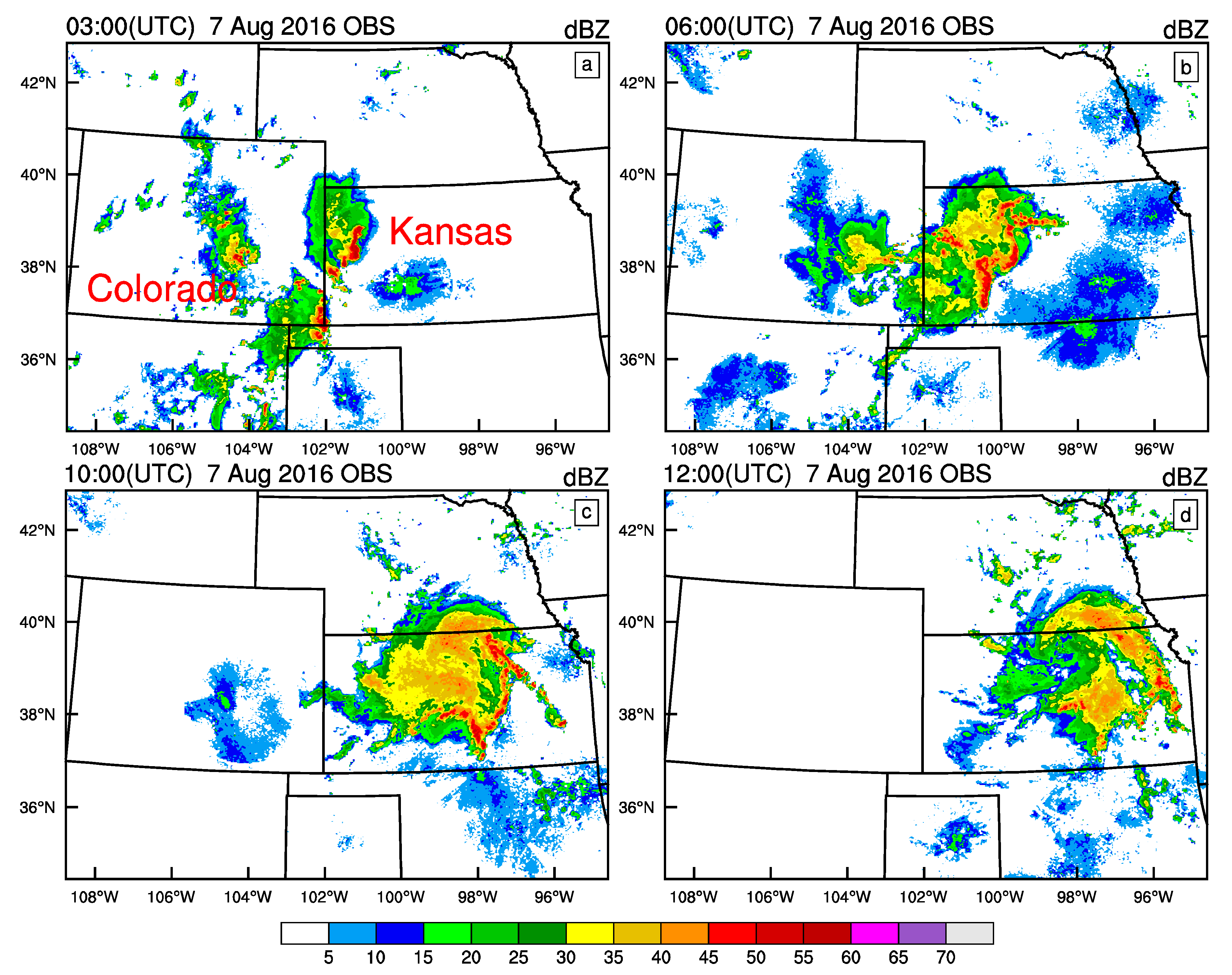
Figure 3.
Outer and inner model domains and locations of 17 radar stations (inverted triangles). Maximum ranges of radars are shown by circles. The radar stations are: KRIW (Riverton, WY), KLNX (North Platte, NE), KOAX (Omaha, NE), KCYS (Cheyenne, WY), KUEX (Hastings, NE), KGJX (Grand Junction, CO), KFTG (Denver, CO), KGLD (Goodland, KS), KTWX (Topeka, KS), KPUX (Pueblo, CO), KDDC (Dodge City, KS), KICT (Wichita, KS), KVNX (Moody AFB, GA), KINX (Tulsa, OK), KABX (Albuquerque, NM), KAMA (Amarillo, TX), and KTLX (Oklahoma, OK).
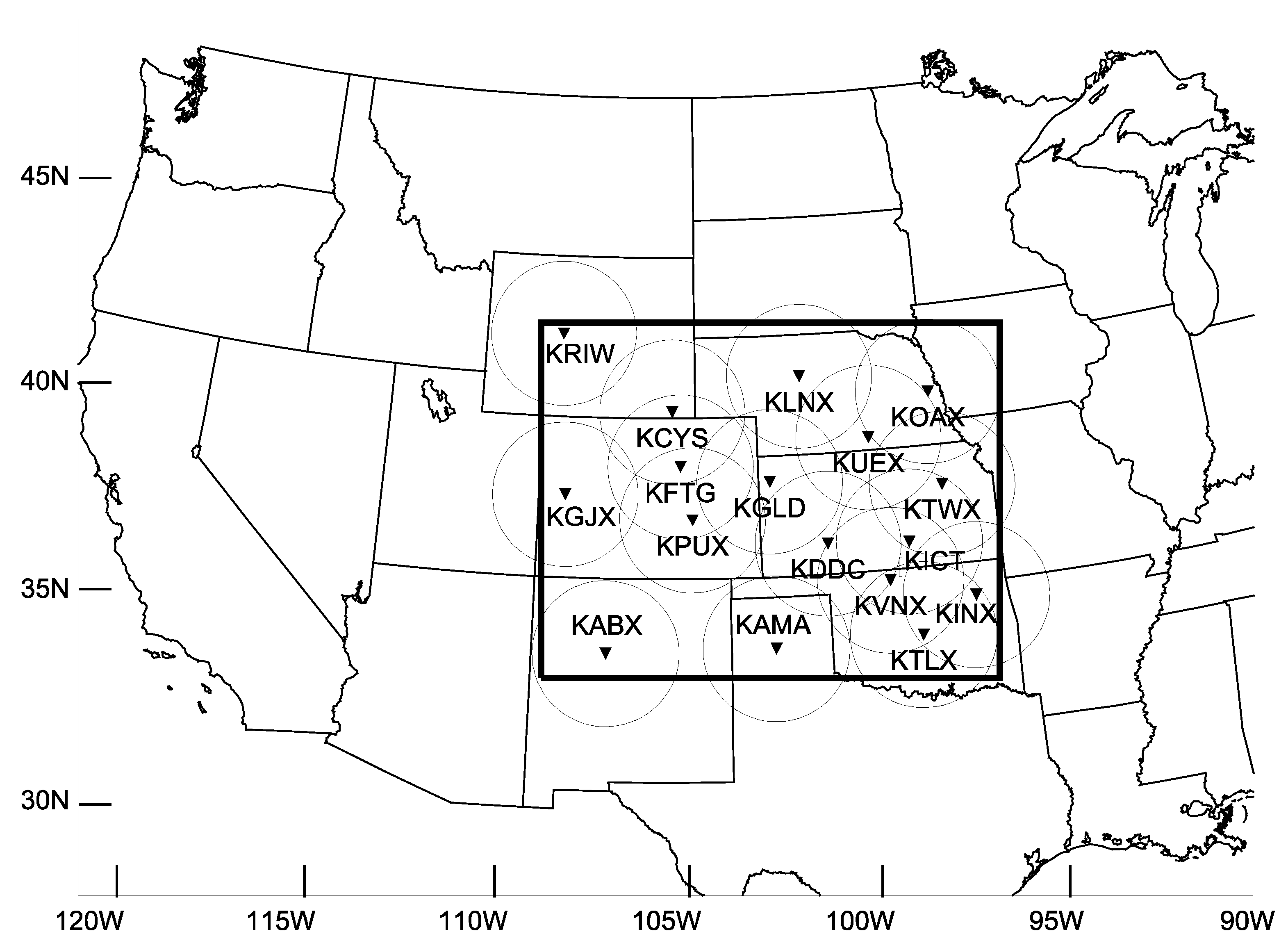
Figure 4.
(a) The locations of 10 radiosondes (blue dots); and (b) 1927 METAR (red dots) stations over the inner region of domain.
Figure 4.
(a) The locations of 10 radiosondes (blue dots); and (b) 1927 METAR (red dots) stations over the inner region of domain.

Figure 5.
Diagram illustrating two-step procedure of radar data assimilation. In Step 1 (red dashed box), conventional observations from Global Telecommunications System (GTS) are assimilated with three-hourly update cycles. In Step 2 (green dashed-box), radar data are assimilated with hourly update cycles.

Figure 6.
The fractions skill score (FSS) (a,d,g); the equitable threat score (ETS) (b,e,h); and probability of detection (POD) (c,f,i) of the Exp3DVC (blue curve), ExpHYBC (orange curve), Exp3DVCR (green curve) and ExpHYBCR (red curve) averaged over seven 0–12 h forecasts (initialized at 15:00, 18:00, 21:00, 00:00, 03:00, 06:00 and 09:00 UTC on 7 August 2016), for precipitation thresholds of 1, 2.5 and 5 mm.

Figure 7.
One-hour accumulated precipitation (unit: mm) of: observation (a); Exp3DVC (b); ExpHYBC (c); Exp3DVCR (d); and ExpHYBCR (e) of the convective system at 05:00 UTC on 7 August 2016 (initialized at 00:00 UTC on 7 August 2016).
Figure 7.
One-hour accumulated precipitation (unit: mm) of: observation (a); Exp3DVC (b); ExpHYBC (c); Exp3DVCR (d); and ExpHYBCR (e) of the convective system at 05:00 UTC on 7 August 2016 (initialized at 00:00 UTC on 7 August 2016).
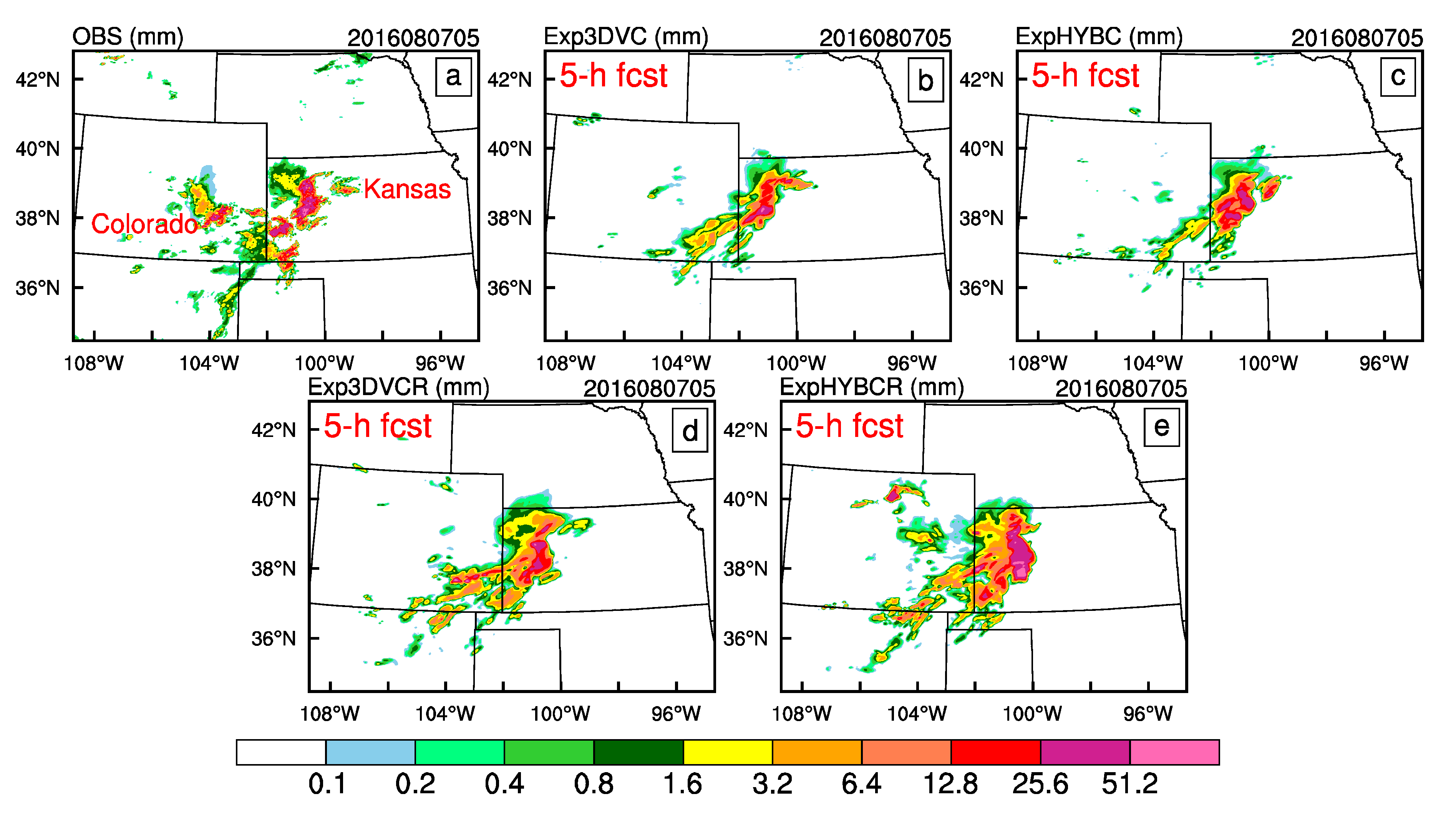
Figure 8.
One-hour accumulated precipitation (unit: mm) of: observation (a); Exp3DVC (b); ExpHYBC (c); Exp3DVCR (d); and ExpHYBCR (e) of the convective system at 06:00 UTC on 7 August 2016 (initialized at 00:00 UTC on 7 August 2016).
Figure 8.
One-hour accumulated precipitation (unit: mm) of: observation (a); Exp3DVC (b); ExpHYBC (c); Exp3DVCR (d); and ExpHYBCR (e) of the convective system at 06:00 UTC on 7 August 2016 (initialized at 00:00 UTC on 7 August 2016).

Figure 9.
One-hour accumulated precipitation (unit: mm) of: observation (a); Exp3DVC (b); ExpHYBC (c); Exp3DVCR (d); and ExpHYBCR (e) of the convective system at 07:00 UTC on 7 August 2016 (initialized at 03:00 UTC on 7 August 2016).
Figure 9.
One-hour accumulated precipitation (unit: mm) of: observation (a); Exp3DVC (b); ExpHYBC (c); Exp3DVCR (d); and ExpHYBCR (e) of the convective system at 07:00 UTC on 7 August 2016 (initialized at 03:00 UTC on 7 August 2016).
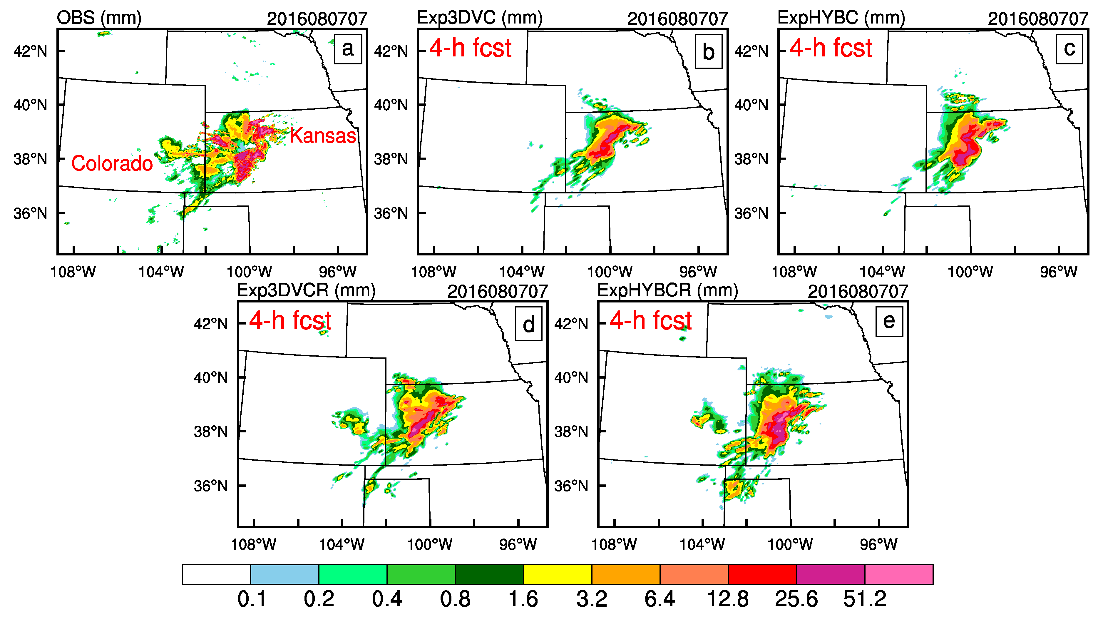
Figure 10.
One-hour accumulated precipitation (unit: mm) of: observation (a); Exp3DVC (b); ExpHYBC (c); Exp3DVCR (d); and ExpHYBCR (e) of the convective system at 09:00 UTC on 7 August 2016 (initialized at 03:00 UTC on 7 August 2016).
Figure 10.
One-hour accumulated precipitation (unit: mm) of: observation (a); Exp3DVC (b); ExpHYBC (c); Exp3DVCR (d); and ExpHYBCR (e) of the convective system at 09:00 UTC on 7 August 2016 (initialized at 03:00 UTC on 7 August 2016).
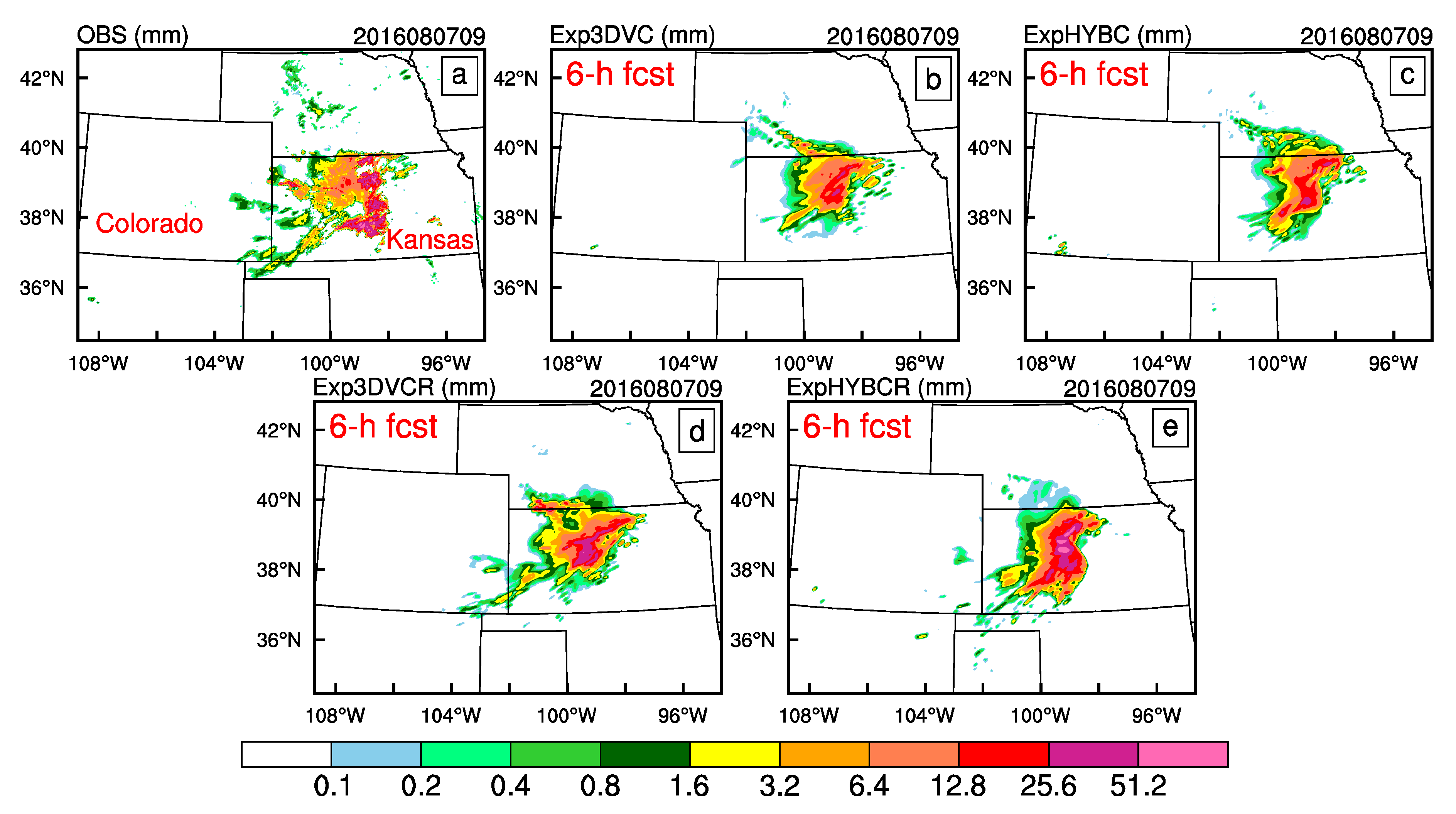
Figure 11.
FSS (a,d,g), ETS (b,e,h) and POD (c,f,i) of Exp3DVC (blue curve), ExpHYBC (orange curve), Exp3DVCR (green curve) and ExpHYBCR (red curve) averaged over seven 0–12 h forecasts (initialized at 15:00, 18:00, 21:00, 00:00, 03:00, 06:00 and 09:00 UTC on 7 August, 2016), for reflectivity thresholds of 5, 15 and 25 dBZ.
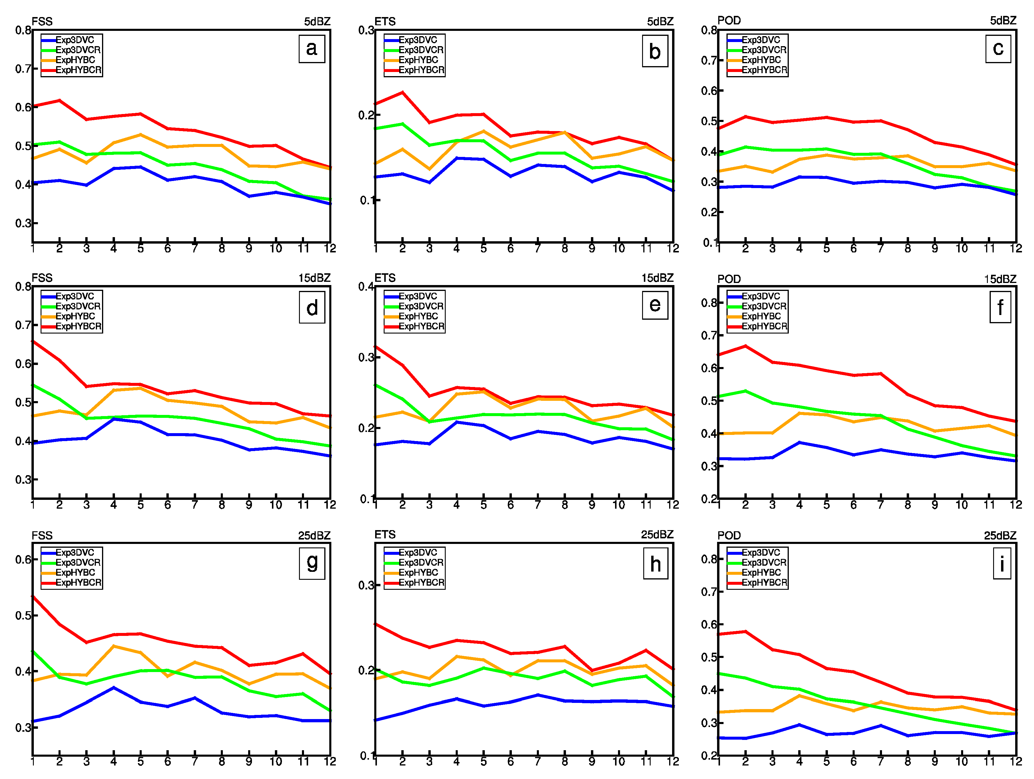
Figure 12.
Composite reflectivity (unit: dBZ) of: observation (a); Exp3DVC (b); ExpHYBC (c); Exp3DVCR (d); and ExpHYBCR (e) of the convective system at 06:00 UTC on 7 August 2016 (initialized at 00:00 UTC on 7 August 2016).
Figure 12.
Composite reflectivity (unit: dBZ) of: observation (a); Exp3DVC (b); ExpHYBC (c); Exp3DVCR (d); and ExpHYBCR (e) of the convective system at 06:00 UTC on 7 August 2016 (initialized at 00:00 UTC on 7 August 2016).
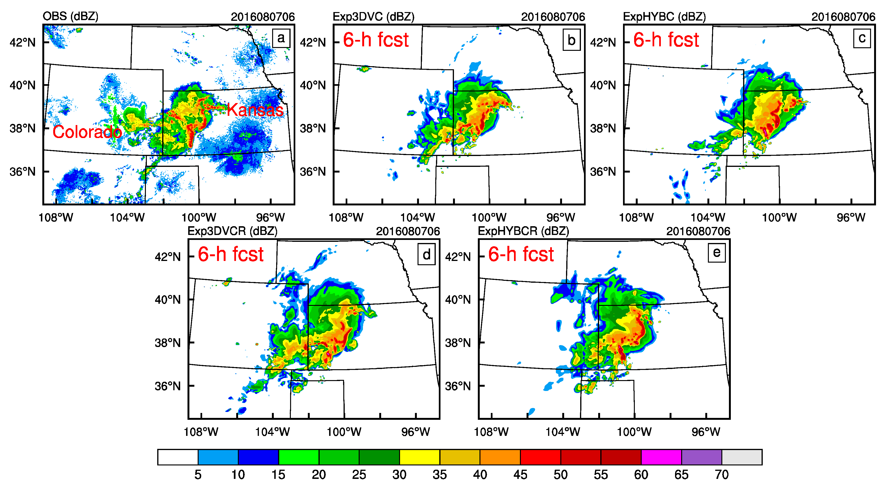
Figure 13.
Composite reflectivity (unit: dBZ) of: observation (a); Exp3DVC (b); ExpHYBC (c); Exp3DVCR (d); and ExpHYBCR (e) of the convective system at 07:00 UTC on 7 August 2016 (initialized at 03:00 UTC on 7 August 2016).
Figure 13.
Composite reflectivity (unit: dBZ) of: observation (a); Exp3DVC (b); ExpHYBC (c); Exp3DVCR (d); and ExpHYBCR (e) of the convective system at 07:00 UTC on 7 August 2016 (initialized at 03:00 UTC on 7 August 2016).
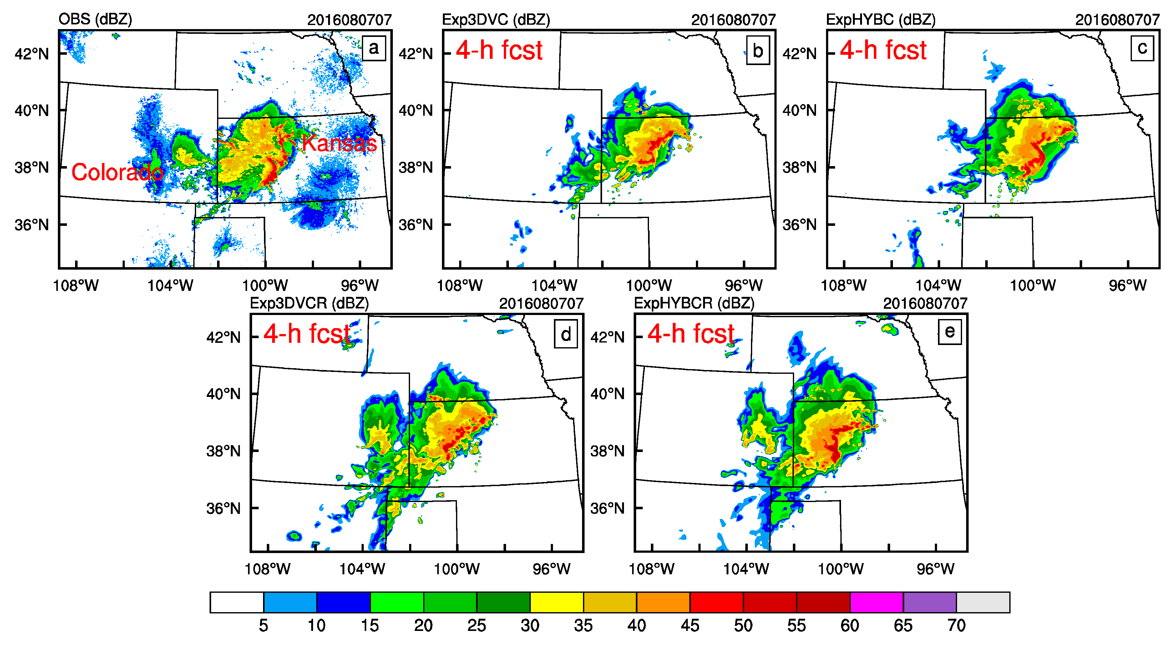
Figure 14.
Vertical -profile of average RMSEs of forecast background against all the radiosondes in the 3-km domain for: (a) u component (unit: m s−1); (b) v component (unit: m s−1); (c) T (unit: °C); and (d) Q (unit: g kg−1), from Exp3DVC (blue curve), ExpHYBC (orange curve), Exp3DVCR (green curve) and ExpHYBCR (red curve).
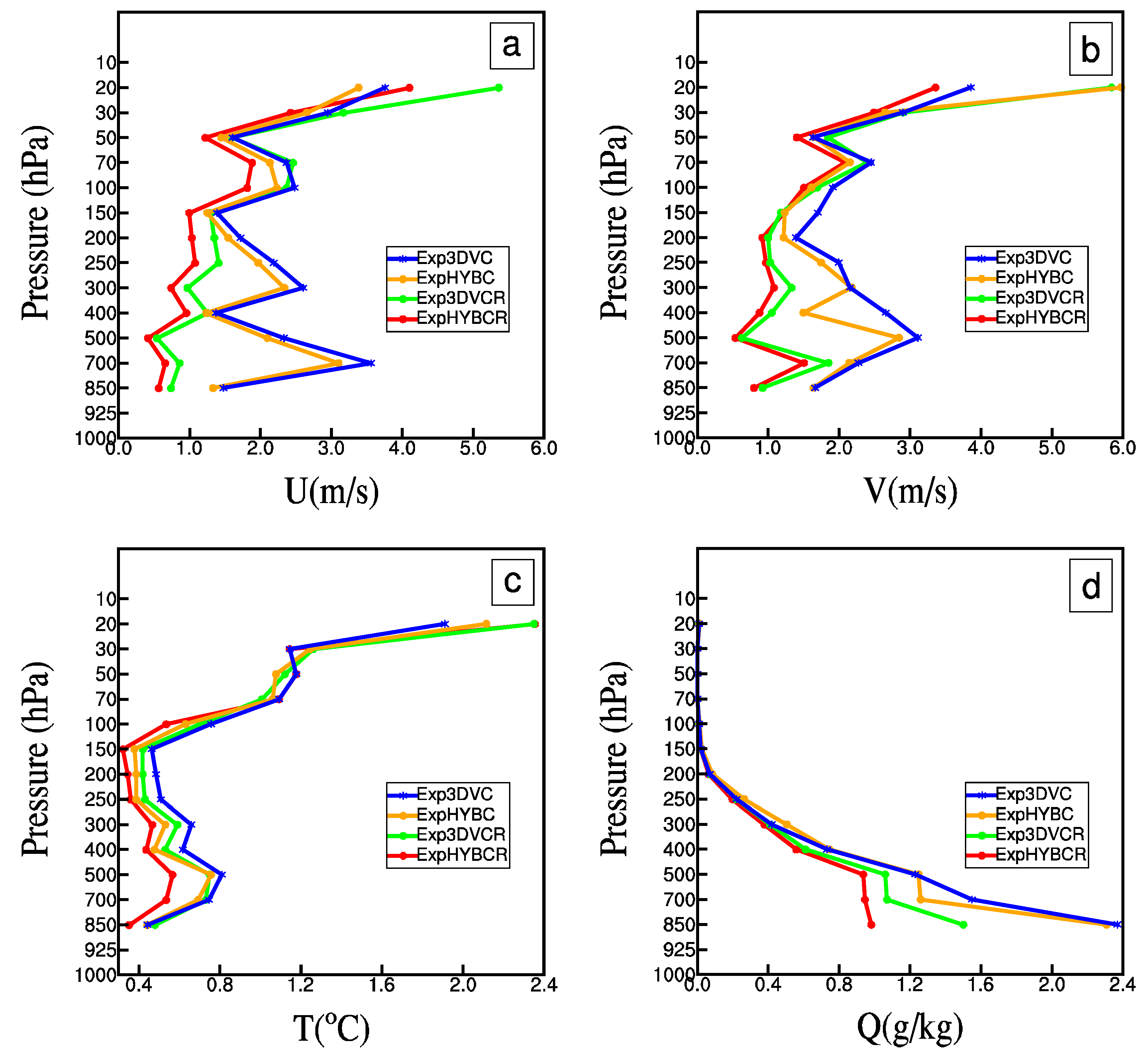
Figure 15.
Average RMSE of forecast background against all the METAR stations in 3-km domain for u component (unit: m s−1), v component (unit: m s−1), T (unit: °C), and Q (unit: g kg−1), from Exp3DVC (blue bar), ExpHYBC (orange bar), Exp3DVCR (green bar) and ExpHYBCR (red bar).
Figure 15.
Average RMSE of forecast background against all the METAR stations in 3-km domain for u component (unit: m s−1), v component (unit: m s−1), T (unit: °C), and Q (unit: g kg−1), from Exp3DVC (blue bar), ExpHYBC (orange bar), Exp3DVCR (green bar) and ExpHYBCR (red bar).
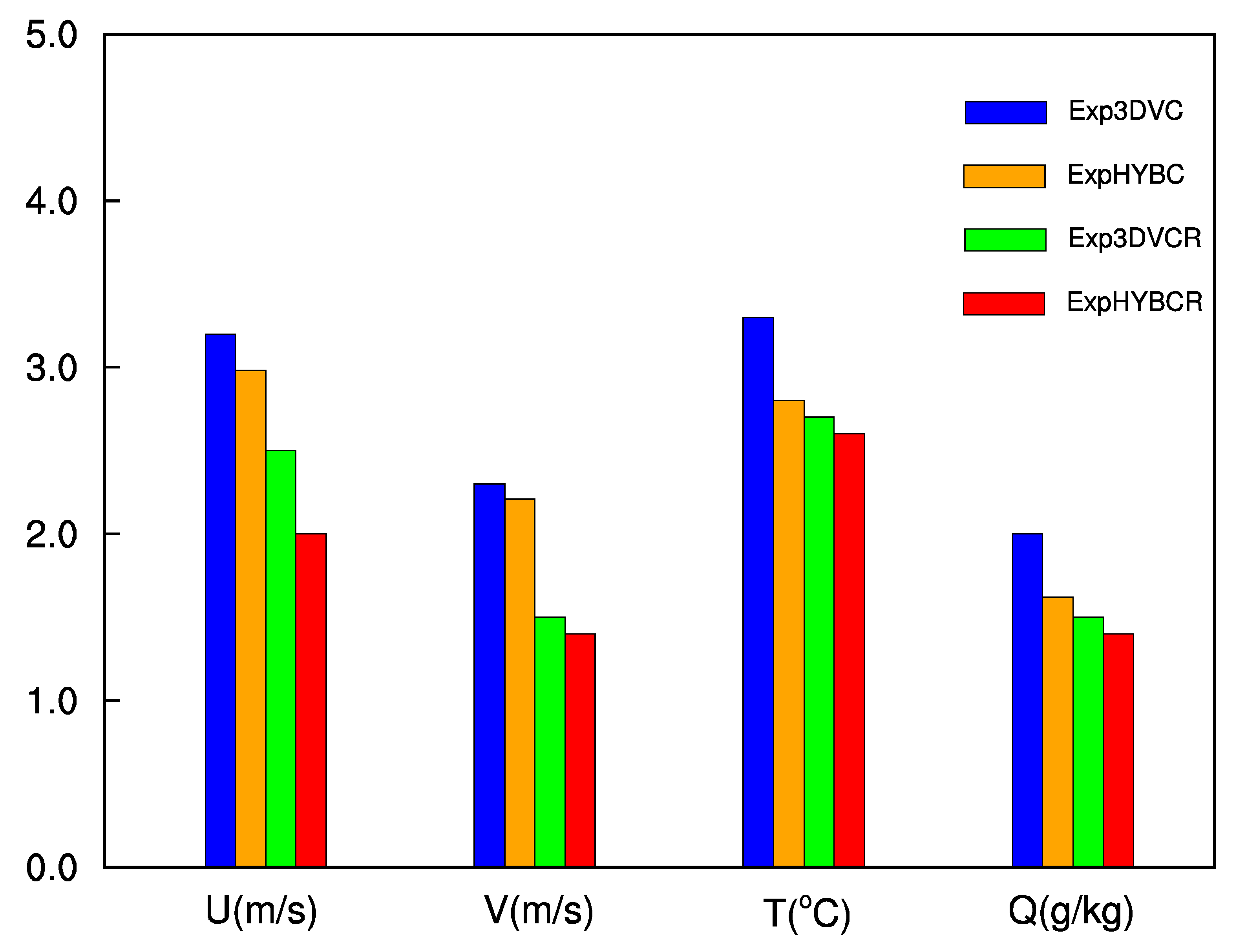
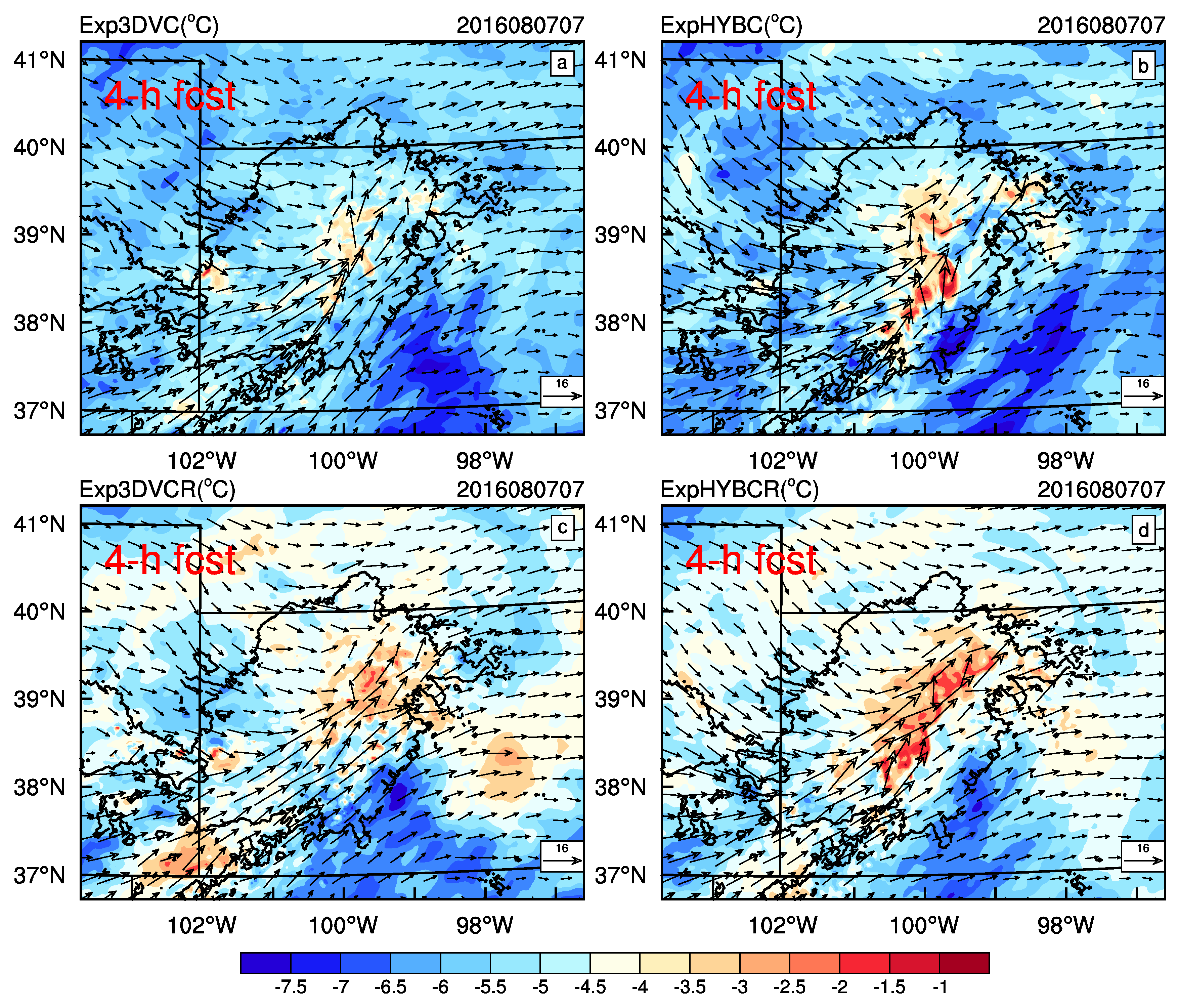
Figure 16.
Surface temperature (unit: °C) and wind (unit: m s−1) of: Exp3DVC (a); ExpHYBC (b); Exp3DVCR (c); and ExpHYBCR (d) of the convective system at 07:00 UTC on 7 August 2016 (initialized at 03:00 UTC on 7 August 2016). Solid black lines represent contours of observed reflectivity exceeding 20 dBZ.

Figure 17.
Temperature (unit: °C) and wind (unit: m s−1) of: Exp3DVC (a); ExpHYBC (b); Exp3DVCR (c); and ExpHYBCR (d) of the convective system at 500 hPa at 07:00 UTC on 7 August 2016 (initialized at 03:00 UTC on 7 August 2016). Solid black lines represent contours of observed reflectivity exceeding 20 dBZ.


Table 1.
List of experiments.
| Experiments | Assimilation method | Assimilation Data |
|---|---|---|
| Exp3DVC | 3DVar | GTS |
| ExpHYBC | hybrid | GTS |
| Exp3DVCR | 3DVar | GTS and Radar |
| ExpHYBCR | hybrid | GTS and Radar |
© 2017 by the authors. Licensee MDPI, Basel, Switzerland. This article is an open access article distributed under the terms and conditions of the Creative Commons Attribution (CC BY) license (http://creativecommons.org/licenses/by/4.0/).
Share and Cite
MDPI and ACS Style
Gao, S.; Huang, D. Assimilating Conventional and Doppler Radar Data with a Hybrid Approach to Improve Forecasting of a Convective System. Atmosphere 2017, 8, 188. https://doi.org/10.3390/atmos8100188
AMA Style
Gao S, Huang D. Assimilating Conventional and Doppler Radar Data with a Hybrid Approach to Improve Forecasting of a Convective System. Atmosphere. 2017; 8(10):188. https://doi.org/10.3390/atmos8100188
Chicago/Turabian StyleGao, Shibo, and Danlian Huang. 2017. "Assimilating Conventional and Doppler Radar Data with a Hybrid Approach to Improve Forecasting of a Convective System" Atmosphere 8, no. 10: 188. https://doi.org/10.3390/atmos8100188
Note that from the first issue of 2016, this journal uses article numbers instead of page numbers. See further details here.