Aerosol Optical Properties over China from RAMS-CMAQ Model Compared with CALIOP Observations
by
Tong Wu
1,2, 
Meng Fan
2,*,
Jinhua Tao
2,*,
Lin Su
2,
Ping Wang
1,
Dong Liu
3, 
Mingyang Li
2,
Xiao Han
4 and
Liangfu Chen
2 1
College of Geomatics, Shandong University of Science and Technology, Qingdao 266000, China
2
State Key Laboratory of Remote Sensing Science, Jointly Sponsored by Institute of Remote Sensing and Digital Earth of Chinese Academy of Sciences and Beijing Normal University, Beijing 100101, China
3
State Key Laboratory of Modern Optical Instrumentation, College of Optical Science and Engineering, Zhejiang University, Hangzhou 310027, China
4
State Key Laboratory of Atmospheric Boundary Layer Physics and Atmosphere Physics, Chinese Academy of Sciences, Beijing 100101, China
*
Authors to whom correspondence should be addressed.
Atmosphere 2017, 8(10), 201; https://doi.org/10.3390/atmos8100201
Submission received: 6 September 2017
/
Revised: 29 September 2017
/
Accepted: 13 October 2017
/
Published: 17 October 2017
(This article belongs to the Special Issue Aerosol Optical Properties: Models, Methods & Measurements)
Abstract
:The horizontal and vertical distributions of aerosol optical properties over China in 2013–2015 were investigated using RAMS (Regional Atmospheric Modeling System)-CMAQ (Models-3 Community Multiscale Air Quality) simulations and CALIOP (Cloud-Aerosol Lidar with Orthogonal Polarization) observations. To better understand the performance of the RAMS-CMAQ model over China, comparisons with the ground-based Sun photometers AERONET (Aerosol Robotic Network), MODIS (Moderate Resolution Imaging Spectroradiometers) data and the on-board Lidar CALIOP were used for comprehensive evaluations, which could characterize the abilities of the model to simulate the spatial and vertical distributions of the AOD (Aerosol Optical Depth) as well as the optical properties for four seasons. Several high value areas (e.g., the Sichuan Basin, Taklamakan Desert, North China Plain, and Yangtze River Delta) were found over China during the study period, with the maximum mean AOD (CALIOP: ~0.7; RAMS-CMAQ: >1) in the Sichuan district. Compared with AODs of AERONET, both the CALIOP and RAMS-CMAQ AODs were underestimated, but the RAMS-CMAQ data show a better correlation with AERONET (AERONET vs. RAMS-CMAQ R: 0.69, AERONET vs. CALIOP R: 0.5). The correlation coefficients between RAMS-CMAQ and CALIOP are approximately 0.6 for all four seasons. The AEC (Aerosol Extinction Coefficient) vertical profiles over major cities and their cross sections exhibit two typical features: (1) most of the AEC peaks occurred in the lowest ~0.5 km, decreasing with increasing altitude; and (2) the RAMS-CMAQ AEC underestimated the region with high AODs in the northwest of China and overestimated the region with high AODs in the east–central plain and the central basin regions. The major difference in the AEC values of RAMS-CMAQ and CALIOP is mainly caused by the level of relative humidity and the hygroscopic growth effects of water-soluble aerosols, especially, in the Sichuan district. In general, both the column and vertical RAMS-CMAQ aerosol optical properties could be supplemented efficiently when satellite observations are not available or invalid over China in the applications of climate change and air pollution.
1. Introduction
Aerosols in the atmosphere play an important role in global climate change, the radiation balance, and particulate pollution. Aerosols affect climate change via scattering or absorbing solar radiation, which directly impacts the global radiation budget. Aerosol particles acting as cloud condensation nuclei can also indirectly affect the radiation budget by modifying the efficiency of droplet freezing, contributing to the modulation of droplet growth, and changing the onset of precipitation in convective clouds [1]. Aerosol optical properties, such as the extinction, scattering, and absorption coefficients, are major factors that influence these radiative effects [2]. According to the Intergovernmental Panel on Climate Change Fifth Assessment Report (IPCC-AR5), the estimation of aerosol-cloud radiative forcing still carries large uncertainties, and the quantification of aerosols and clouds in climate models continues to be a challenge [3]. One important uncertainty in regional or global climate is derived from the optical properties of the aerosols and their vertical distribution in the atmosphere [4]. Changes in the vertical distribution of aerosols can modify the vertical profiles of the radiative heating in the atmosphere and can further influence the stability of the atmosphere [5]. Performing multi-instrumental measurements to investigate the aerosol optical properties and radiative transfer is efficient in Saharan dust [6,7].
Both passive and active satellite sensors can be used for aerosol detection from space. Passive sensors such as MODIS on NASA’s Terra and Aqua satellites are based on the modification of the solar radiation field induced by aerosol particles and have been used for decades. Levy et al. introduced the MODIS Collection 6 (C6) algorithm to retrieve the AODs over different surface types and showed the improvements that the C6 algorithm made over both oceans and land [8]. Ginoux et al. presented a global-scale high-resolution map of dust sources based on the MODIS deep blue aerosol products [9]. Kim et al. investigated the seasonal, monthly and geographical variations of columnar aerosol optical properties over East Asia through MODIS, MPL (micro-pulse LIDAR), and AERONET measurements [10]. In recent years, especially since the launch of CALIOP on board the CALIPSO (Cloud-Aerosol Lidar and Infrared Pathfinder Satellite Observation) platform in 2006, many studies with focus on the aerosol vertical distribution were published. The CALIOP LIDAR provides active remote sensing both during day and nighttime retrievals to characterize changes in the aerosol and cloud properties. The aerosol subtypes of the CALIOP measurements and the AERONET daily aerosol types were compared by Mielonen et al., and they found that 70% of the CALIOP and AERONET aerosol types were in agreement [11]. Huang et al. investigated the aerosol vertical transport processes in Asia using the CALIOP and surface measurements, and their results showed the dust and pollution moved from the Taklamakan and Gobi deserts to the Pacific Ocean via westerly jets [12]. Chen et al. developed a dust aerosol detection method by combining the CALIOP active Lidar and passive IIR measurements, and this method could significantly reduce misclassification rates to as low as ~7% for the active dust season [13]. Still, because of the low signal-to-noise ratios and the low temporal resolution, the wider applications of CALIPSO observations are limited [14].
The chemistry and transport numerical models are keys to capturing aerosol optical properties and aerosol radiative forcing. In the past decades, some modeling of aerosol distributions and the climate-related aerosol effects has been conducted. Zhang et al. developed the RAMS-CMAQ (Regional Atmospheric Modeling System-Community Multiscale Air Quality) model to analyze the nitrate aerosol concentration distributions of the seasons and regions over East Asia and showed a strong agreement between the model simulations and the observations [15]. Han et al. investigated the aerosol optical properties using RAMS-CMAQ in East Asia, and their modeled AOD results showed a strong agreement with AERONET, CSHNET (Chinese Sun Hazemeter Network) and MODIS observations [16]. Using the WRF-Chem (Weather Research and Forecasting model coupled to Chemistry) model in Mexico City, Li et al. investigated the variations in and spatial distributions of aerosol concentrations, and the WRF-Chem with a non-traditional 2-product secondary organic aerosol (SOA) showed a distinct superiority in predicting organic aerosols [17]. Heald et al. compared the vertical profiles of the atmospheric organic aerosols with the GEOS-CHEM (Goddard Earth Observing System coupled to Chemistry) model-simulated distribution and found that GEOS-CHEM can generally accurately reflect the organic aerosol vertical profiles [18]. However, due to the lack of aerosol vertical profile observations, most of the modeling systems were discussed and validated via column-averages rather than via vertical layered aerosol properties. In addition, many studies of the aerosol vertical distributions are based on ground-based data. So it is worth noting that these studies are limited by the site location.
Here, we used the RAMS-CMAQ data to investigate the column and vertical distributions of aerosol optical properties over China in 2013–2015. To illustrate the applicability of RAMS-CMAQ aerosol parameters in different regions and different seasons, CALIOP, MODIS, and AERONET aerosol observations were employed for comprehensive evaluations. Section 2 describes the RAMS-CMAQ and CALIOP data, and the details of data processing. The results and analysis are shown in Section 3. A comparison of the results of RAMS-CMAQ, CALIOP, and AERONET is given in Section 3.1 to verify the accuracy of the model and satellite results in the area. Section 3.2 and Section 3.3, respectively, show the spatial distributions of AOD and the vertical extinction profiles properties. Section 4 is the summary and conclusions.
2. Data and Methodology
2.1. RAMS-CMAQ Data
2.1.1. RAMS-CMAQ Model
The air quality modeling system RAMS-CMAQ has been used to investigate the regional atmospheric pollution and environment issues in many studies [16]. The regional model CMAQs can simulate various chemical and physical processes that are significant for understanding atmospheric trace gas transformation and distribution [19]. The ISORROPIA (Regional Particulate Model and the thermodynamic equilibrium model) were used in this study [20,21]. RAMS is the highly versatile numerical code applied to provide the meteorological fields for CMAQ. The background meteorological fields and sea surface temperature were obtained from the European Center for Medium-Range Weather Forecasts reanalysis datasets with 1° × 1° spatial resolutions.
For the source emissions, the anthropogenic sources included many pollutants, such as SO2 and nitrogen oxides (NOX), which were obtained from the 0.5° × 0.5° spatial resolution monthly mean inventory that was prepared to support the MICS-Asia II (Model Intercomparison Study Asia Phase II) [22]. The biomass burning emission sources comprise forest burning, savanna/grassland burning and crop residues burning and were provided by the global monthly mean inventory from Advanced Very High Resolution Radiometer satellite monitoring data with 0.5° × 0.5° spatial resolutions [23]. The natural hydrocarbon emissions and nitrogen oxide emissions from soil were provided by the Global Emissions Inventory Activity global monthly inventory [24]. Aside from the nitrogen oxides mentioned earlier, the other natural sources of nitrogen oxides were obtained from MICS-Asia II and the Emission Database for Global Atmospheric Research [25]. The dust and sea salt emissions were provided by Han et al. [26] and Gong [27]. The Model of Ozone and Related Tracers (MOZART-4) field data provided the boundary information [28].
2.1.2. RAMS-CMAQ 550 nm AOD Calculation
Here, the RM (reconstructed mass-extinction) method is employed to calculate the AOD derived from RAMS-CMAQ. The AOD at a specific wavelength is obtained by integrating the aerosol extinction coefficient from the surface to the top of the atmosphere. The extinction coefficient, , is thought of as the following sum:
where is the aerosol scattering coefficient with the unit , is the aerosol absorption coefficient with the unit , is the gas scattering coefficient with the unit , and is the gas absorption coefficient with the unit . Because the natural oxygen and nitrogen molecules cause the Rayleigh scattering, we neglect in this study. The magnitudes of the gas particulates have insignificant contributions to gaseous absorptions at 550 nm, so we also neglect in this study [29]. The formula used in this study is as follows:
where the top and base are the aim layers’ top and base. In this study, we use the RM to get the aerosol scattering and absorption coefficients for the extinction coefficient calculation.
where within the equation brackets are the mass concentration in . , , and are sulfate, nitrate, and ammonium; is the organic mass; is the fine soil; is the coarse mass; and is the light-absorbing carbon. The specific scattering coefficients, 0.003, 0.004, 0.001, 0.0006, and 0.01, in Equation (2) with the unit of , are based on an assumption of a lognormal particle size distribution [30]. The relative humidity-based aerosol scattering enhancement factor is obtained from the studies of Malm et al. [30]. The previous comparison study of Biswadev et al. showed the feasibility of deriving the aerosol optical property using the RM from the atmospheric model-simulated data [29].
2.2. CALIOP Data
The CALIOP, which is aboard the CALIPSO satellite, is an elastic backscatter LIDAR that transmits polarized laser light at 532 and 1064 nm [31]. The LIDAR signal inversion begins at approximately 30 km above the ground and continues to the surface. Its orbit repeats every 16 days [32].
The Level 2 aerosol and cloud products V4 (version 4.10) over China from January 2013 to December 2015 are used in this study. V4 represents a substantial advance over V3 and earlier releases; known retrieval artifacts have been eliminated, and numerous enhancements have been incorporated to increase the accuracy of the data while simultaneously reducing uncertainties [33]. Both the daytime and nighttime profiles are obtained. Here, several quality control conditions of the data files are used to filter the data. The atmosphere volume description is used to screen out clouds and to identify bad profiles. CAD (Cloud-Aerosol Discrimination) is used to indicate the confidence of features identified as clouds or aerosols. To identify the cloud-free aerosol features with high confidence, the CAD scores inclusive of −20 and −100 are used. The Extinction_QC_Flag_532 (Ext_QC) summarize the final states of the extinction retrieval. When the Ext_QC = 0 or 1, the profile is regarded as a good one. Each aerosol extinction profile in the Level 2 products has some uncertainty [34] and a profile with an extinction uncertainty score of 99.9 is regarded as unreliable. Because of the daytime background solar illumination, the Extinction_Coefficient_532 with scores of less than −0.2 were removed [35].
2.3. Data Processing
All the CALIOP Level 2 aerosol and cloud products (daytime and nighttime), hourly RAMS-CMAQ aerosol componential data, AERONET data and MOD/MYD04 10 km AOD products over China span the period from 2013 to 2015. To investigate the reliability of the CALIOP retrievals and the RAMS-CMAQ simulations, these data were compared with the ground-based sun photometer measurements from AERONET. Because of the gap in the spatial scale between the CALIOP and AERONET observations, and according to the studies of Omar et al. and Liu et al., the AERONET observations within 2 h of the CALIOP overpass were averaged in a circle with a radius of 40 km around each AERONET site [36,37]. Similarly, the corresponding temporal and spatial ranges of the AERONET and RAMS-CMAQ results were 1 h and 40 km, respectively.
To compare the CALIOP-retrieved data and the RAMS-CMAQ simulations, the satellite data and model data were matched for the CALIOP overpass time. These data were analyzed for four periods: spring (March, April and May, MAM); summer (June, July and August, JJA); autumn (September, October and November, SON); and winter (December, January and February, DJF).
The spatial comparison of the column AOD values from CALIOP and RAMS-CMAQ used the MODIS 10 km AODs as references. Because of the spatial resolutions and the low frequencies of CALIOP, the column AODs from the satellite observations and the model simulations were resampled to a lower resolution (1° × 1° grid cell). For a comparison of the vertical information, the CALIOP and simulated vertical profile data height is limited to 10 km [38,39]. The daily vertical profile information was averaged over the nearest grid cell. The vertical cross sections drawn over the longitude and latitude were derived from consecutive vertical profiles.
3. Results and Analysis
3.1. AOD Validation Using AERONET Data
AERONET AODs with Level 2 and Level 1.5 were used to evaluate the reliabilities of both the CALIPSO observations and RAMS-CMAQ simulations from 2013 to 2015. In this paper, there are seven AERONET sites (i.e., Beijing, Xianghe, Beijing_CAMS, Beijing_RADI, Hong Kong_PolyU, Xu Zhou_CUMT and Hong Kong_Sheung) over China (Table 1). The overall and seasonal comparisons of the AERONET AODs with the CALIOP-retrieved AODs and RAMS-CMAQ-simulated values are shown in Figure 1. In addition, the corresponding statistical results are listed in Table 2, including the R, RMSE, mean, slope and intercept for overall and seasonal data. Due to the low temporal resolution and the narrow width of the CALIOP observations, the quantity of selected CALIOP data is much lower than for the RAMS-CMAQ data. Therefore, the CALIOP and RAMS-CMAQ data matched to the AERONET AOD are not in complete agreement in terms of their dates, times and locations. The CALIOP or RAMS-CMAQ data that satisfied the filter rules mentioned in Section 2.3 are used for the calculation of the monthly AOD means. Overall, there are 124 monthly records of the CALIOP-retrieved AODs, and 209 monthly values of the RAMS-CMAQ-simulated AODs over China from 2013 to 2015. Comparing the monthly AOD means of the CALIOP-retrieved and RAMS-CMAQ-simulated data results in a correlation coefficient R of 0.5 and an RMSE of 0.04. Our study indicates that the RAMS-CMAQ-simulated AOD performs better than the CALIOP-retrieved AOD. The correlation coefficient between AERONET and RAMS-CMAQ reaches 0.69, and the RMSE is only 0.022.
According to the seasonal results of the comparison (Figure 1 and Table 2), both the monthly CALIOP-retrieved and RAMS-CMAQ-simulated AODs of the summer show the highest correlations (R = 0.58 for CALIOP and R = 0.78 for RAMS-CMAQ) with the ground-based AERONET measurements. The slopes are 0.536 and 0.277, and the intercepts are 0.147 and 0.186 for RAMS-CMAQ and CALIOP, respectively. The lowest correlation coefficients exist in the autumn, i.e., 0.47 and 0.44 for CALIOP and RAMS-CMAQ, respectively. In most cases, the CALIOP-retrieved AODs are lower, which might be caused by the low temporal resolution and cloud interruption, especially when the AERONET AOD values are larger than 0.5 in the autumn. Moreover, both for the monthly CALIOP-retrieved and RAMS-CMAQ-simulated AODs, the data in the spring and winter are more significantly undervalued than those in the summer and autumn. In addition, both the CALIOP (spring: 0.114, winter: 0.056) and RAMS-CMAQ (spring: 0.046, winter: 0.054) data have large AOD RMSEs. Based on our analysis, the AODs retrieved from the CALIOP observations were smaller than those from the AERONET AOD measurements, which is consistent with the studies of Omart et al. [36,40]. Although the RAMS-CMAQ-simulated AODs have better agreement with the AERONET AOD values, some underestimates exist over China.
3.2. Spatial Distributions of AODs
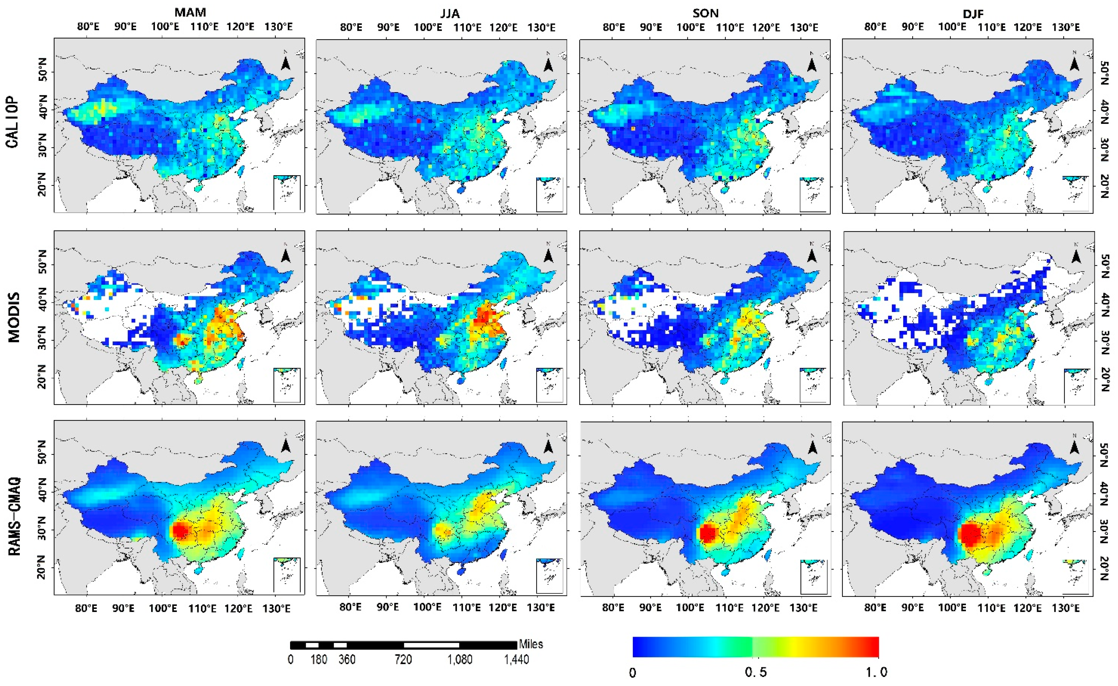
The seasonal spatial distributions of the AODs are shown in Figure 2. Because of the remarkable differences in the AODs of CALIOP and RAMS-CMAQ over some regions in China, the MODIS 10 km AOD was used as a standard reference to assess the potential for characterizing the spatial distributions using both the CALIOP and RAMS-CMAQ data. According to Figure 2, the four highlighted regions (i.e., the Sichuan Basin, Taklamakan Desert, North China Plain, and Yangtze River Delta) with high AOD values are all monitored or simulated by CALIOP and RAMS-CMAQ. In general, comparing the MODIS 10 km AODs with the CALIOP AODs shows that the latter are lower for the four seasons, while the RAMS-CMAQ simulated AODs are higher, especially in the Sichuan Basin.
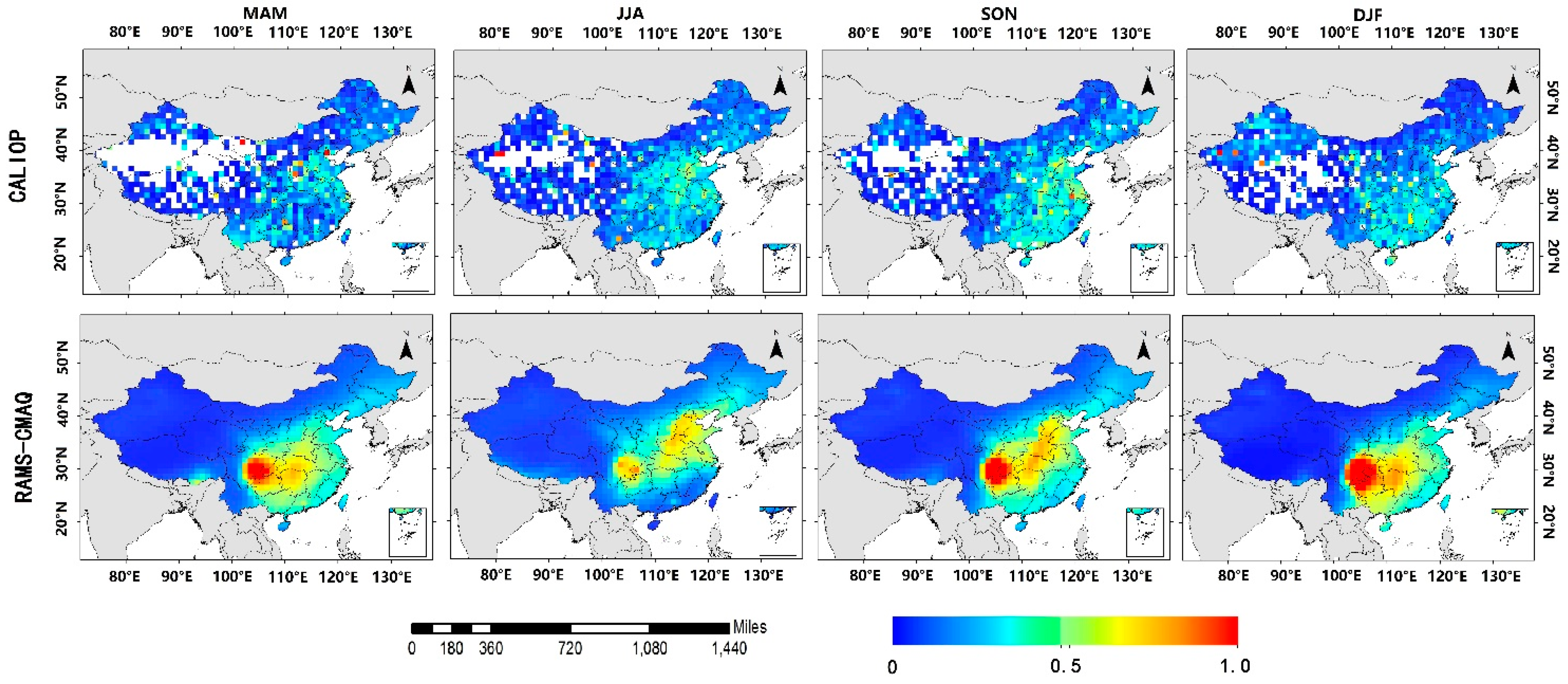
The Sichuan district (~103° E, ~30° W) is the region with the greatest differences in the seasonal AODs from CALIOP and RAMS-CMAQ, where the model-simulated AODs are much higher, and the satellite-retrieved AODs are lower. This situation may occur for two reasons. One reason is the complicated geographic location of the Sichuan Basin. The Sichuan Basin is in the middle south of China with a highland in the west of the basin. The complex terrain results in complex weather patterns and increases the complexities of satellite retrievals and model simulations. Large amounts of clouds and aerosols are present in the Sichuan district year round. When we screened the data, only the data without clouds were used. Although the CAD filter was used for the data screening, over-screening also occurred due to the low SNR (signal-to-noise ratio) [41]. CALIOP’s low time resolution and the over-screening in the data processing caused the number of effective CALIOP observations to be small, so the simulated AOD values are higher than the CALIOP observed results in some area, especially in the spring, fall and winter. The second reason has to do with the computing method of the RAMS-CMAQ. The model AODs are taken as relative to the particulate concentrations, and some of the particulates have hygroscopic growth. The complex terrain makes the relative humidity and the particulate concentrations in the Sichuan Basin higher than those in other regions. Because both CALIOP and RAMS-CMAQ can provide aerosol component information, different componential AODs were computed to identify the specific aerosol components, introducing large errors to the AOD results. As shown in Figure 2, the areas with RAMS-CMAQ column AOD values greater than 1 are larger than those of CALIOP and MODIS, especially in the spring, autumn and winter. Compared with the AOD results of CALIOP and MODIS, the RAMS-CMAQ column AODs were overestimated by 0.4–0.6 and 0.15–0.45. In this paper, the CALIOP AODs of clean continental and polluted continental aerosols, which are used as the water-soluble component, were chosen to match the sum of the RAMS-CMAQ AODs of sulfate, nitrate and ammonium (Figure 3). Figure 3 shows that the RAMS-CMAQ water-soluble AODs are greatly higher in the CALIOP results. The water-soluble AODs of RAMS-CMAQ are approximately 0.4–0.8 higher than those of CALIOP. The CALIOP AOD of smoke aerosols was used to match the RAMS-CMAQ AOD of black carbon, and the sum of the CALIOP AOD of dust and polluted dust aerosols was used to match the RAMS-CMAQ AOD of dust, which is not shown here because of the small differences in these AODs. Figure 2 and Figure 3 show that the differences in the AODs of CALIOP and RAMS-CMAQ over the Sichuan Basin are mainly caused by the AOD of the water-soluble component, which accounts for the largest contribution to the total column AOD. In RAMS-CMAQ, the water-soluble component AOD is largely overvalued. However, the feature of the high AODs in this region is not captured by the water-soluble component AOD of CALIOP.
In eastern China, especially in the North China Plain and Yangtze River Delta Region, the results of the comparison of the CALIOP observations and RAMS-CMAQ simulations are highly relevant. In the middle district, compared with the satellite results, the model results show an overestimation, and such an overestimation obviously occurs in the autumn (SON) and winter (DJF). The study of Liu et al. also proved that the CALIOP seasonal column AOD is lower in the middle of China, especially in the autumn and winter [42], which may be due to the low time resolution and the low SNR of CALIOP.
In western China, especially in the Taklamakan Desert, the RAMS-CMAQ-simulated seasonal AODs are lower than the CALIOP observations. The seasonal AODs dominated by the dust aerosols over the desert region are much larger than those over the other areas in western China. This phenomenon is obvious in the desert area, especially in the spring (form March to May), as is shown in Figure 2 [16]. A similar tendency is also shown in the RAMS-CMAQ simulation results, although the RAMS-CMAQ-simulated AOD values are lower compared to the observed results.
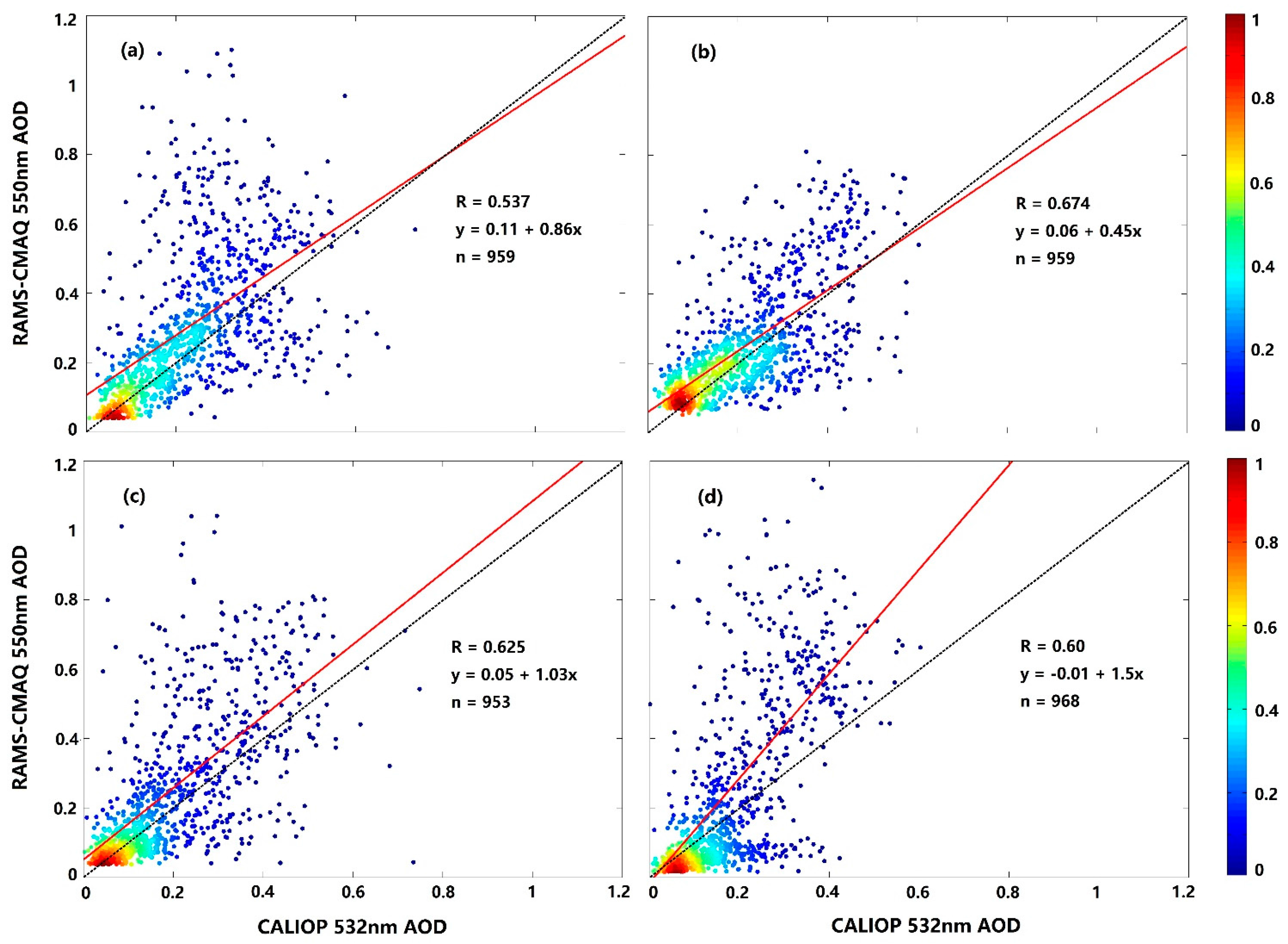
To quantitatively evaluate the column AOD results of CALIOP and RAMS-CMAQ, scatter diagrams are shown in Figure 4. Although the RAMS-CMAQ 550 nm AOD is generally slightly higher, there is a strong agreement between the CALIOP measurements and model simulations. In addition, most of the AODs of both CALIOP and RAMS-CMAQ focus on the ranges of 0–0.3 for the four seasons. As shown in Figure 4a, the correlation coefficient of the spring (R = 0.54) is lower than those of the other seasons, where the record number of matched AODs is 959, and most values are lower than 0.4. The overestimations of the RAMS-CMAQ-simulated AODs (greater than 0.6) exist in the Sichuan Basin, while the underestimations of the AODs are mainly less than 0.4 over the Taklamakan Desert. Summer is the season with the highest R (0.67) and the lowest overvalued level of RAMS-CMAQ-simulated AODs (Figure 4b), which indicates the smallest difference in the AODs of CALIOP and RAMS-CMAQ. The slope of Figure 4c is 1.03, meaning that the model values are greater than those observed. In the winter, the phenomenon of overestimation is very significant due to the high AODs over the Sichuan Basin and the middle of China in the RAMS-CMAQ model.
3.3. Vertical Distribution of Extinction Properties
3.3.1. Vertical Extinction Profiles of the Major Cities of China
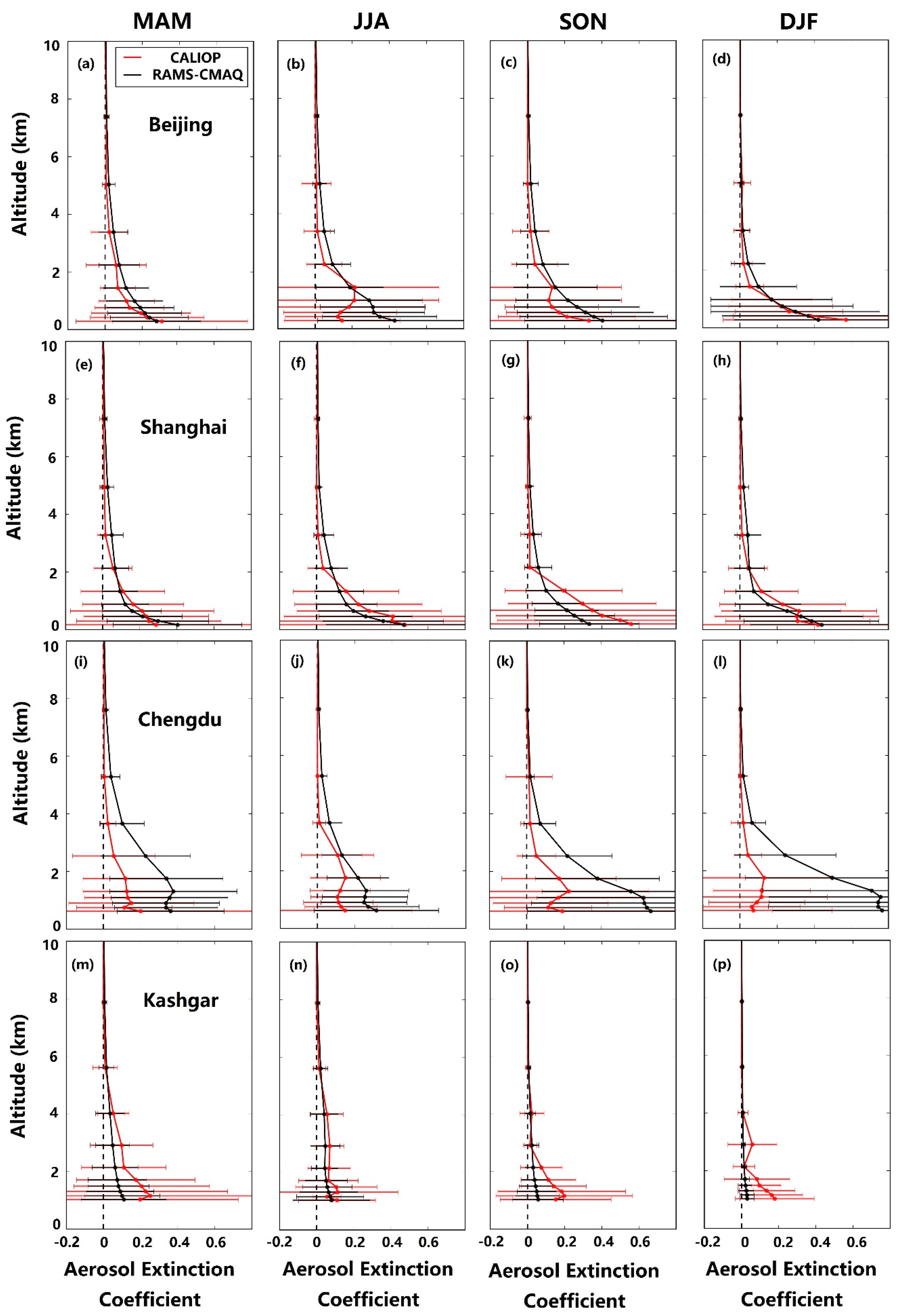
The AEC profiles from the CALIOP retrievals are used to evaluate the ability of RAMS-CMAQ to characterize the vertical distributions of aerosols in China. Figure 5 and Figure 6 depict the seasonal AEC profiles of eight regionally representative cities of China. Both for the total and low atmospheres, the CALIOP seasonal AEC profiles agree well with the RAMS-CMAQ ones of Beijing and Shanghai in eastern China (Figure 5), and the standard deviation values (SDV), which show the variability of the vertical profiles of RAMS-CMAQ, are generally smaller than those of CALIOP. For Beijing city (Figure 5a–d), the peaks in the CALIOP seasonal AEC profiles are located close to the surface at altitudes of ~100 m in the spring, autumn and winter (0.3 km−1–0.4 km−1). Additionally, the SDVs are similar for CALIOP and RAMS-CMAQ for heights below 1.8 km in the autumn (CALIOP: 0.3 km−1–0.5 km−1; RAMS-CMAQ: 0.25 km−1–0.4 km−1) and winter (CALIOP: 0.24 km−1–0.6 km−1; RAMS-CMAQ: 0.35 km−1–0.5 km−1). The model simulation reproduced such features of the AEC well for both the vertical distribution and the magnitude, especially in the winter. However, there are significant differences in the AEC profile of CALIOP and RAMS-CMAQ in the low atmosphere (lower than 1 km) in the summer, and the RAMS-CMAQ-simulated AECs are larger than those of CALIOP. For Shanghai city (Figure 5e–h), the RAMS-CMAQ AEC profiles also agree well with the CALIOP results. Both the model and the satellite profile peaks of the four seasons are located at an altitude near 0.4 km−1. The SDVs below 1.7 km are much greater, especially for the CALIOP seasonal profiles. The maximum CALIOP AEC SDV is greater than 0.5 km−1. However, the RAMS-CMAQ maximum AEC SDV is approximately 0.4 km−1 at the same altitude.
In addition to the column AOD, the overestimation of the RAMS-CMAQ AEC profile in the middle of China is much greater than those in the other regions of China, especially in Sichuan Basin. Here, Chengdu City is chosen as a typical representation of the middle of China. The differences in the AEC profiles of CALIOP and RAMS-CMAQ are mainly focused below the height of 6 km (Figure 5i–l). For the AEC profile in the summer, the peak of the CALIOP AEC (approximately 0.18 km−1) is near a height of 2 km, which is slightly higher than that of the RAMS-CMAQ simulation (approximately 0.3 km−1). In the autumn and winter, the RAMS-CMAQ-simulated AECs in the low atmosphere are greater than 0.5 km−1, while the CALIOP-retrieved AECs are only approximately 0.25 and 0.15 km−1, respectively. The SDVs of the two seasons are extremely large at a height of 1.8 km (max CALIOP SDV value: approximately 0.4 km−1; max RAMS-CMAQ SDV value: approximately 0.6 km−1), meaning that the high levels of relative humidity and the hygroscopic growth effects of water-soluble aerosols introduce large uncertainties into the model simulations of the column AODs and the AEC profiles over the Sichuan Basin.
The seasonal AEC profiles obtained from the RMAS-CMAQ model are shown to be underestimated when compared to the satellite observations over the Taklamakan Desert area (Figure 5m–p), which is similar to the results of the AODs. In this region, the maximum CALIOP seasonal AECs are approximately 0.2 km−1 and occur near the surface. In the spring, the CALIOP SDV is much greater than that of RAMS-CMAQ at the altitudes of 1.5 km–1.9 km. The maximum CALIOP SDV value reaches 0.6 km−1, which is much greater than that of RAMS-CMAQ (approximately 0.2 km−1). Moreover, the CALIOP seasonal AEC changes significantly with decreasing altitudes, which is not well simulated by RMAS-CMAQ. For Urumchi and Lhasa, both the vertical distributions and the magnitudes of the seasonal RMAS-CMAQ AECs are consistent with the CALIOP AECs due to the low levels of air pollution in western China. The seasonal vertical profiles of the AECs in Shenyang (northern China, Figure 6a–d) and Fuzhou (southeastern China, Figure 6e–h) are also well matched between the CALIOP measurements and the RAMS-CMAQ simulated results for heights greater than 1 km. The high SDVs are mainly focused in the altitudes below 1.6 km in Fuzhou. The max SDVs in Fuzhou appear close to the max AEC values (max CALIOP SDV: 0.35 km−1–0.4 km−1; max RAMS-CMAQ SDV: 0.25 km−1–0.3 km−1) in the four seasons. Overall, the maximums in the AEC profiles are mainly located in the lowest atmosphere over the eastern region of China. For most regions of China, RAMS-CMAQ could provide acceptable AEC profiles, even over the Tibetan Plateau. Because of the complex air pollution conditions in the Sichuan Basin, the worst performance of the AEC profile simulations of RAMS-CMAQ is in this region, and when compared with the satellite observations, the RAMS-CMAQ results are largely overestimated. For the SDVs of the AEC profiles, the high values are almost all focused at heights ranging from the land surface to 1.5 km, and the model-simulated SDVs are smaller than the satellite-derived SDVs.
3.3.2. Cross Sections of the Vertical Aerosol Distribution over China
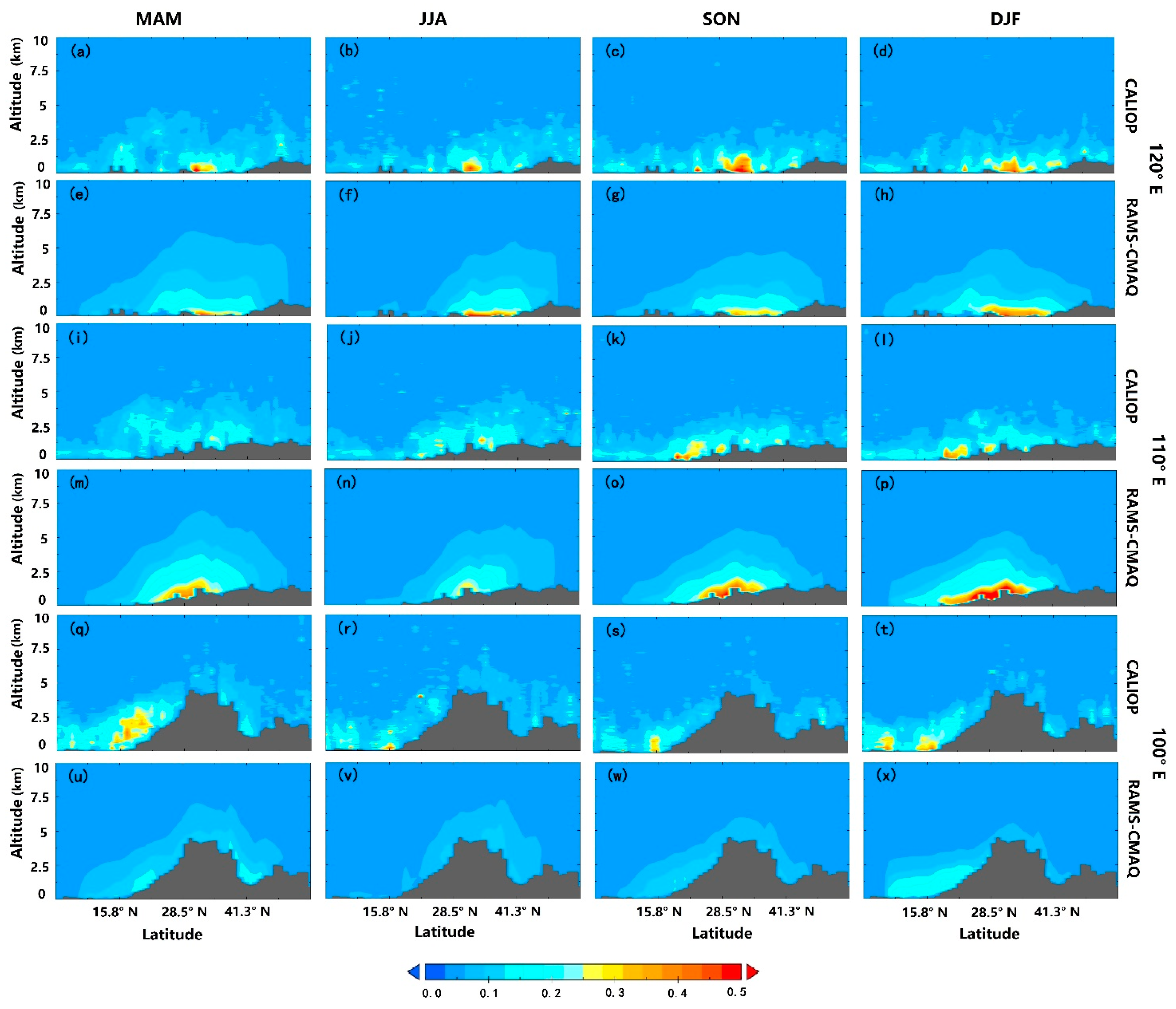
The CALIOP-retrieved and RAMS-CMAQ-simulated cross sections of the AEC profiles over China for the latitudes of 40° N and 30° N and the longitudes of 120° E, 110° E and 100° E were obtained to analyze the variations in the continuous distributions in different seasons (Figure 7 and Figure 8). Note that the selected longitudes and latitudes cross many of the typical economic regions, including the Beijing-Tianjin-Hebei region and Yangtze River Delta region, and cover many regions with different terrains, such as the Tibetan Plateau, the North China Plain, and the Sichuan Basin. Therefore, the cross sections of the AEC profiles in Figure 7 and Figure 8 could largely describe the general characteristics of the AEC vertical distributions over China. Figure 9 and Figure 10 described the main AEC vertical distribution differences between the RMAS-CMAQ and CALIOP values over China.
The cross section of the AEC profile at the latitude of 30° N (Figure 7a–h and Figure 9a–d) passes through the Yangtze River Delta region, the Sichuan Basin and the Tibetan Plateau. The maximum height in Figure 7a–h is the Tibetan Plateau, which is located near 104° E. Both the model-simulated and satellite-retrieved results showed that the AEC values (approximately 0.1 km−1) of the Tibetan Plateau (<100° E) are not as high as those in other places, especially for the values in the low atmosphere (below 2 km), which is mainly due to the high terrain and the low concentration of aerosol particles. On the eastern side of the Tibetan Plateau, there are two regions with high AEC values that correspond to the Sichuan Basin (102° E–107° E) and the Yangtze River Delta (118° E–123° E) region, respectively.
Figure 9a–d show that the overestimations of RAMS-CMAQ mainly occur in the middle of China (102° E–107° E). The RAMS-CMAQ AECs are higher than those of CALIOP in all four seasons. The RAMS-CMAQ AECs are 0.1–0.25 km−1 in the spring and summer and 0.1–0.5 km−1 in autumn and winter. At the latitude of 40° N in Figure 7i–p and Figure 9e–h, the cross section passes over the Taklamakan Desert and Beijing-Tianjin-Hebei region at longitudes below 90° E and eastern China at one above 105° E. Note that at 40° N the high AEC (approximately 0.25 km−1) area is mainly focused over the west of China (82° E–94° E). However, the RAMS-CMAQ underestimates this area. Figure 9e–h show that the underestimated values are approximately 0.2 km−1.
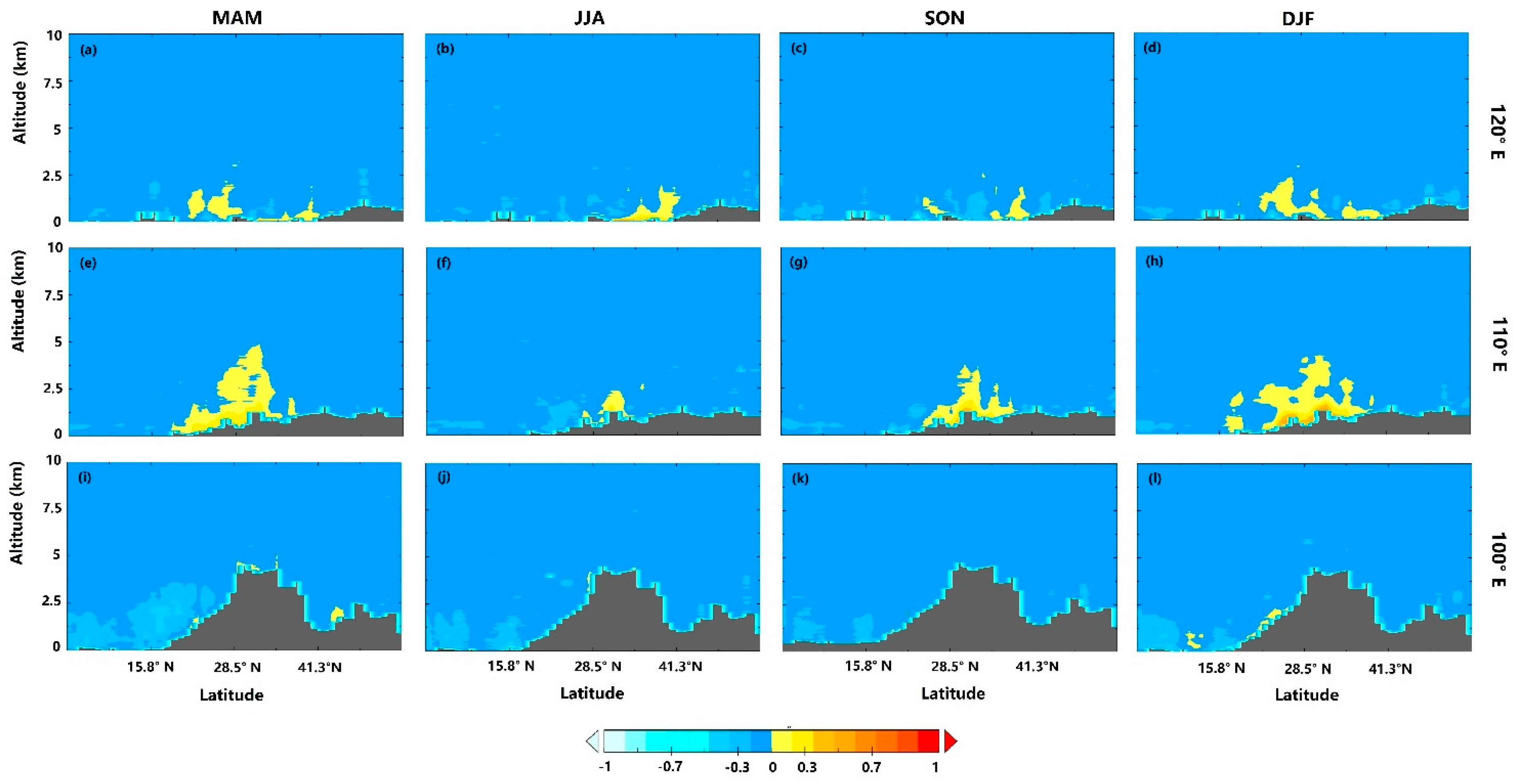
In Figure 8a–h and Figure 10a–d, the longitude 120° E is in eastern China. The cross section of the AEC profile at the longitude of 120° E covered most of the areas with large anthropogenic aerosol sources in eastern China, such as the Yangtze River Delta region and the Shandong Peninsula. Regardless of the differences between the model and the satellite results, the areas characterized with high AEC values near the surface (<0.5 km) in Figure 8a–h are mainly located around the latitudes of 30° N–33° N. By comparing the CALIOP-retrieved and the RAMS-CMAQ-simulated cross sections of the AEC profiles, the RAMS-CMAQ results are shown to accurately simulate the major features of the AEC profiles over China. The areas with the largest differences between CALIOP-retrieved and RAMS-CMAQ-simulated AEC profiles are concentrated between 25° N and 40° N (Figure 10a–d). In these areas, the RAMS-CMAQ-simulated AEC values are 0.1 km−1 higher than the CALIOP-retrieved AECs. The cross section at the longitude 110° E (Figure 8i–p and Figure 10e–h mainly crosses the middle of China. At this cross section, although the RAMS-CMAQ overestimates the AEC profiles at ~30° N at the altitudes of 0.5 km–2.5 km, the RAMS-CMAQ can well describe the AEC tendencies. Figure 10e–h showed that the overestimations are serious in the spring and winter, and the overestimated values are ~0.2 km−1. The 100° E cross section shown in Figure 8q–x and Figure 10i–l passes through western China (100° E, 23° N–43° N). Both the RAMS-CMAQ and CALIOP AEC values in this region are low (RAMS-CMAQ AEC: ~0.2 km−1; CALIOP AEC: ~0.35 km−1). Additionally, because of the unique topography of this region, the differences in the AECs are not as large as those in other areas (around ~0.3 km−1).
The above comparison of the CALIOP retrievals and the RAMS-CMAQ simulations demonstrates that the model is generally able to reproduce the major features of the AEC distributions over China in both the horizontal and vertical directions. Compared with the CALIOP cross sections, the areas underestimated by RAMS-CMAQ are mainly focused in western China, while the higher areas are focused in the east–central plains and central basin.
4. Conclusions
The air quality modeling system RAMS-CMAQ and CALIOP data were used in this paper to investigate and evaluate the three-dimensional distribution of the aerosol optical properties over China in 2013–2015. The comparison between the AERONET data and the RAMS-CMAQ-simulated and CALIOP data showed that both the model and the satellite results generally underestimate the actual values for all four seasons. The RAMS-CMAQ-simulated results have higher correlations with the AERONET data (AERONET vs RAMS-CMAQ R: 0.69, AERONET vs. CALIOP R: 0.5).
The spatial distributions of AODs over China showed that the CALIOP-retrieved AOD, the RAMS-CMAQ-simulated AOD and the MODIS 10 km AOD have generally similar tendencies. The high value areas are concentrated in the Sichuan Basin, Taklamakan Desert, North China Plain and Yangtze River Delta. However, the RAMS-CMAQ-simulated AODs are overestimated (CALIOP: 0.4–0.6; MODIS: 0.15–0.45) in the Sichuan Basin and underestimated in the Taklamakan Desert when compared with the CALIOP-retrieved values. The correlation coefficients between the model and satellite results are approximately 0.6 in all four seasons. The RAMS-CMAQ data can roughly simulate the AOD spatial distributions except for over the central basin, where the AOD values are overestimated by approximately 0.5 km−1 when compared with those of CALIOP.
The cross section of the AEC values and profiles in the vicinity of some of the major cities in China showed the similar tendencies of the satellite profiles and model profiles. In addition, two typical features are quite obvious: most of the AEC peaks occurred near the surface, at ~0.5 km above the ground, and decrease with increasing altitudes, as observed over Beijing and Shanghai; and the RAMS-CMAQ AECs underestimated the areas of focus of northwestern China (approximately 0.1 km−1 less than the satellite observations) and overestimated the areas of focus over the east-central plain and the central basin (approximately 0.3 km−1 greater than those observed by the satellite) near the ground. The high SDVs (approximately 0.2 km−1–0.6 km−1) mostly occurred at 1.5 km above the surface. Longitude/latitude–altitude cross sections of AECs from RAMS-CMAQ and CALIOP showed the major features of the vertical AEC distribution over the typical areas of China. Combined with the previous analyses, we find that the AEC values are dependent on both the particle concentrations and relative humidity and are more obvious in the model results.
Generally, the space-based Lidar CALIOP measurements provided the AOD values and aerosol optical properties in three dimensions, which were excellent datasets for the validation and interpretation of model results. The AOD spatial distributions of CALIOP and RAMS-CMAQ were largely the same in most cases. The vertical profile of AEC is dependent on the profiles of both the aerosol concentrations and relative humidity levels. Both the column and vertical RAMS-CMAQ aerosol data are beneficial: in case satellite data observations are missing or invalid, these two data sources could be used as an efficient and effective supplement. The effects of water uptake and internal mixture should treated using Kohler theory and Maxwell–Garnett mixing rule respectively, which will be added in the scheme of RAMS-CMAQ by Dr. Xiao Han to improve the simulation accuracy of aerosol optical properties.
Acknowledgments
This study was supported by the National Key Research and Development Program of China (Grant No. 2016YFC0200404) and the National Natural Science Foundation of China (Grant No. 41501373 and No. 41571347). The authors are grateful to the CALIPSO (https://www-calipso.larc.nasa.gov/), AERONET (https://aeronet.gsfc.nasa.gov/), and MODIS (https://lance.modaps.eosdis.nasa.gov/) scientific team for the provision of satellite data utilized in this study. We are also grateful to the State Key Laboratory of Atmospheric Boundary Layer Physics and Atmosphere Physics for providing the RAMS-CMAQ data.
Author Contributions
Tong Wu designed the experiment, collected data, applied the analysis method, and wrote this paper; Meng Fan and Jinhua Tao conceived of the experiment and revised the paper; Lin Su, Ping Wang, Liangfu Chen, Dong Liu and Mingyang Li provided technical guidance and revised the paper; Xiao Han provided technical guidance for the RAMS-CMAQ data.
Conflicts of Interest
The authors declare no conflict of interest.
References
- Kaufman, Y.J.; Tanre, D.; Boucher, O. A satellite view of aerosols in the climate system. Nature 2002, 419, 215–223. [Google Scholar] [CrossRef] [PubMed]
- Hess, M.; Koepke, P.; Schult, I. Optical properties of aerosols and clouds: The software package opac. Bull. Am. Meteorol. Soc. 1998, 79, 831–844. [Google Scholar] [CrossRef]
- Wild, M.; Folini, D.; Schar, C.; Loeb, N.; Dutton, E.G.; Konig-Langlo, G. The global energy balance from a surface perspective. Clim. Dyn. 2013, 40, 3107–3134. [Google Scholar] [CrossRef]
- Chaikovsky, A.; Dubovik, O.; Holben, B.; Bril, A.; Goloub, P.; Tanre, D.; Pappalardo, G.; Wandinger, U.; Chaikovskaya, L.; Denisov, S.; et al. Lidar-radiometer inversion code (LiRIC) for the retrieval of vertical aerosol properties from combined lidar/radiometer data: Development and distribution in earlinet. Atmos. Measure. Tech. 2016, 9, 1181–1205. [Google Scholar] [CrossRef] [Green Version]
- Li, J.X.; Yin, Y.; Li, P.R.; Li, Z.Q.; Li, R.J.; Cribb, M.; Dong, Z.P.; Zhang, F.; Li, J.; Ren, G.; et al. Aircraft measurements of the vertical distribution and activation property of aerosol particles over the loess plateau in China. Atmos. Res. 2015, 155, 73–86. [Google Scholar] [CrossRef]
- Perrone, M.R.; Tafuro, A.M.; Kinne, S. Dust layer effects on the atmospheric radiative budget and heating rate profiles. Atmos. Environ. 2012, 59, 344–354. [Google Scholar] [CrossRef]
- Guerrero-Rascado, J.L.; Olmo, F.J.; Aviles-Rodriguez, I.; Navas-Guzman, F.; Perez-Ramirez, D.; Lyamani, H.; Arboledas, L.A. Extreme saharan dust event over the southern iberian peninsula in september 2007: Active and passive remote sensing from surface and satellite. Atmos. Chem. Phys. 2009, 9, 8453–8469. [Google Scholar] [CrossRef]
- Levy, R.C.; Mattoo, S.; Munchak, L.A.; Remer, L.A.; Sayer, A.M.; Patadia, F.; Hsu, N.C. The collection 6 modis aerosol products over land and ocean. Atmos. Measure. Tech. 2013, 6, 2989–3034. [Google Scholar] [CrossRef]
- Ginoux, P.; Prospero, J.M.; Gill, T.E.; Hsu, N.C.; Zhao, M. Global-scale attribution of anthropogenic and natural dust sources and their emission rates based on modis deep blue aerosol products. Rev. Geophys. 2012, 50. [Google Scholar] [CrossRef]
- Kim, S.W.; Yoon, S.C.; Kim, J.; Kim, S.Y. Seasonal and monthly variations of columnar aerosol optical properties over east asia determined from multi-year modis, lidar, and aeronet sun/sky radiometer measurements. Atmos. Environ. 2007, 41, 1634–1651. [Google Scholar] [CrossRef]
- Mielonen, T.; Arola, A.; Komppula, M.; Kukkonen, J.; Koskinen, J.; de Leeuw, G.; Lehtinen, K.E.J. Comparison of caliop level 2 aerosol subtypes to aerosol types derived from aeronet inversion data. Geophys. Res. Lett. 2009, 36. [Google Scholar] [CrossRef]
- Huang, J.; Minnis, P.; Chen, B.; Huang, Z.W.; Liu, Z.Y.; Zhao, Q.Y.; Yi, Y.H.; Ayers, J.K. Long-range transport and vertical structure of asian dust from calipso and surface measurements during pacdex. J. Geophys. Res. 2008, 113. [Google Scholar] [CrossRef]
- Chen, B.; Huang, J.; Minnis, P.; Hu, Y.; Yi, Y.; Liu, Z.; Zhang, D.; Wang, X. Detection of dust aerosol by combining CALIPSO active lidar and passive IIR measurements. Atmos. Chem. Phys. 2010, 10, 4241–4251. [Google Scholar] [CrossRef] [Green Version]
- Kacenelenbogen, M.; Vaughan, M.A.; Redemann, J.; Hoff, R.M.; Rogers, R.R.; Ferrare, R.A.; Russell, P.B.; Hostetler, C.A.; Hair, J.W.; Holben, B.N. An accuracy assessment of the caliop/calipso version 2/version 3 daytime aerosol extinction product based on a detailed multi-sensor, multi-platform case study. Atmos. Chem. Phys. 2011, 11, 3981–4000. [Google Scholar] [CrossRef]
- Zhang, M.G.; Gao, L.J.; Ge, C.; Xu, Y.P. Simulation of nitrate aerosol concentrations over east asia with the model system RAMS-CMAQ. Tellus. B Chem. Phys. Meteorol. 2007, 59, 372–380. [Google Scholar] [CrossRef]
- Han, X.; Zhang, M.G.; Zhu, L.Y.; Xu, L.R. Model analysis of influences of aerosol mixing state upon its optical properties in east asia. Adv. Atmos. Sci. 2013, 30, 1201–1212. [Google Scholar] [CrossRef]
- Li, G.; Zavala, M.; Lei, W.; Tsimpidi, A.P.; Karydis, V.A.; Pandis, S.N.; Canagaratna, M.R.; Molina, L.T. Simulations of organic aerosol concentrations in mexico city using the WRF-chem model during the MCMA-2006/milagro campaign. Atmos. Chem. Phys. 2011, 11, 3789–3809. [Google Scholar] [CrossRef] [Green Version]
- Heald, C.L.; Coe, H.; Jimenez, J.L.; Weber, R.J.; Bahreini, R.; Middlebrook, A.M.; Russell, L.M.; Jolleys, M.; Fu, T.M.; Allan, J.D.; et al. Exploring the vertical profile of atmospheric organic aerosol: Comparing 17 aircraft field campaigns with a global model. Atmos. Chem. Phys. 2011, 11, 12673–12696. [Google Scholar] [CrossRef]
- Byun, D.; Schere, K.L. Review of the governing equations, computational algorithms, and other components of the models-3 community multiscale air quality (CMAQ) modeling system. Appl. Mech. Rev. 2006, 59, 51–77. [Google Scholar] [CrossRef]
- Binkowski, F.S.; Shankar, U. The regional particulate matter model.1. Model description and preliminary results. J. Geophys. Res. Atmos. 1995, 100, 26191–26209. [Google Scholar] [CrossRef]
- Nenes, A.; Pandis, S.N.; Pilinis, C. Continued development and testing of a new thermodynamic aerosol module for urban and regional air quality models. Atmos. Environ. 1999, 33, 1553–1560. [Google Scholar] [CrossRef]
- Carmichael, G.R.; Sakurai, T.; Streets, D.; Hozumi, Y.; Ueda, H.; Park, S.U.; Fung, C.; Han, Z.; Kajino, M.; Engardt, M.; et al. MICS-Asia II: The model intercomparison study for asia phase II methodology and overview of findings. Atmos. Environ. 2008, 42, 3468–3490. [Google Scholar] [CrossRef]
- Streets, D.G.; Bond, T.C.; Carmichael, G.R.; Fernandes, S.D.; Fu, Q.; He, D.; Klimont, Z.; Nelson, S.M.; Tsai, N.Y.; Wang, M.Q.; et al. An inventory of gaseous and primary aerosol emissions in Asia in the year 2000. J. Geophys. Res. Atmos. 2003, 108. [Google Scholar] [CrossRef]
- Benkovitz, C.M.; Scholtz, M.T.; Pacyna, J.; Tarrason, L.; Dignon, J.; Voldner, E.C.; Spiro, P.A.; Logan, J.A.; Graedel, T.E. Global gridded inventories of anthropogenic emissions of sulfur and nitrogen. J. Geophys. Res. Atmos. 1996, 101, 29239–29253. [Google Scholar] [CrossRef]
- Olivier, J.G.J.; Bouwman, A.F.; Vandermaas, C.W.M.; Berdowski, J.J.M. Emission database for global atmospheric research (EDGAR). Environ. Monit. Assess. 1994, 31, 93–106. [Google Scholar] [CrossRef] [PubMed]
- Han, Z.W.; Ueda, H.; Matsuda, K.; Zhang, R.J.; Arao, K.; Kanai, Y.; Hasome, H. Model study on particle size segregation and deposition during Asian dust events in March 2002. J. Geophys. Res. Atmos. 2004, 109. [Google Scholar] [CrossRef]
- Gong, S.L. A parameterization of sea-salt aerosol source function for sub- and super-micron particles. Glob. Biogeochem. Cycles 2003, 17. [Google Scholar] [CrossRef]
- Pfister, G.G.; Emmons, L.K.; Hess, P.G.; Lamarque, J.F.; Thompson, A.M.; Yorks, J.E. Analysis of the Summer 2004 ozone budget over the United States using Intercontinental Transport Experiment Ozonesonde Network Study (IONS) observations and Model of Ozone and Related Tracers (MOZART-4) simulations. J. Geophys. Res. Atmos. 2008, 113. [Google Scholar] [CrossRef]
- Roy, B.; Mathur, R.; Gilliland, A.B.; Howard, S.C. A comparison of CMAQ-based aerosol properties with improve, MODIS, and aeronet data. J. Geophys. Res. Atmos. 2007, 112. [Google Scholar] [CrossRef]
- Malm, W.C.; Sisler, J.F.; Huffman, D.; Eldred, R.A.; Cahill, T.A. Spatial and seasonal trends in particle concentration and optical extinction in the united-states. J. Geophys. Res. Atmos. 1994, 99, 1347–1370. [Google Scholar] [CrossRef]
- Stephens, G.L.; Vane, D.G.; Boain, R.J.; Mace, G.G.; Sassen, K.; Wang, Z.E.; Illingworth, A.J.; O'Connor, E.J.; Rossow, W.B.; Durden, S.L.; et al. The cloudsat mission and the a-train—A new dimension of space-based observations of clouds and precipitation. Bull. Am. Meteorol. Soc. 2002, 83, 1771–1790. [Google Scholar] [CrossRef]
- Li, J.W.; Han, Z.W. Aerosol vertical distribution over east China from RIEMS-chem simulation in comparison with calipso measurements. Atmos. Environ. 2016, 143, 177–189. [Google Scholar] [CrossRef]
- Liu, Z.Y.; Winker, D.; Omar, A.; Vaughan, M.; Kar, J.; Trepte, C.; Hu, Y.X.; Schuster, G.; Young, S. Aerosol optical properties above opaque water clouds derived from the caliop version 4 level 1 data. In Proceedings of the 27th International Laser Radar Conference, New York, NY, USA, 5–10 July 2015; Volume 119. [Google Scholar]
- Young, S.A.; Vaughan, M.A.; Kuehn, R.E.; Winker, D.M. The retrieval of profiles of particulate extinction from cloud-aerosol lidar and infrared pathfinder satellite observations (CALIPSO) data: Uncertainty and error sensitivity analyses. J. Atmos. Ocean. Technol. 2013, 30, 395–428. [Google Scholar] [CrossRef]
- Winker, D.M.; Tackett, J.L.; Getzewich, B.J.; Liu, Z.; Vaughan, M.A.; Rogers, R.R. The global 3-d distribution of tropospheric aerosols as characterized by caliop. Atmos. Chem. Phys. 2013, 13, 3345–3361. [Google Scholar] [CrossRef]
- Omar, A.H.; Winker, D.M.; Tackett, J.L.; Giles, D.M.; Kar, J.; Liu, Z.; Vaughan, M.A.; Powell, K.A.; Trepte, C.R. Caliop and aeronet aerosol optical depth comparisons: One size fits none. J. Geophys. Res. Atmos. 2013, 118, 4748–4766. [Google Scholar] [CrossRef]
- Liu, Z.Y.; Vaughan, M.; Winker, D.; Kittaka, C.; Getzewich, B.; Kuehn, R.; Omar, A.; Powell, K.; Trepte, C.; Hostetler, C. The calipso lidar cloud and aerosol discrimination: Version 2 algorithm and initial assessment of performance. J. Atmos. Ocean. Technol. 2009, 26, 1198–1213. [Google Scholar] [CrossRef]
- Papagiannopoulos, N.; Mona, L.; Alados-Arboledas, L.; Amiridis, V.; Baars, H.; Binietoglou, I.; Bortoli, D.; D'Amico, G.; Giunta, A.; Guerrero-Rascado, J.L.; et al. Calipso climatological products: Evaluation and suggestions from earlinet. Atmos. Chem. Phys. 2016, 16, 2341–2357. [Google Scholar] [CrossRef]
- Yu, H.B.; Chin, M.; Winker, D.M.; Omar, A.H.; Liu, Z.Y.; Kittaka, C.; Diehl, T. Global view of aerosol vertical distributions from calipso lidar measurements and gocart simulations: Regional and seasonal variations. J. Geophys. Res. Atmos. 2010, 115. [Google Scholar] [CrossRef]
- Park, R.S.; Song, C.H.; Han, K.M.; Park, M.E.; Lee, S.S.; Kim, S.B.; Shimizu, A. A study on the aerosol optical properties over east Asia using a combination of cmaq-simulated aerosol optical properties and remote-sensing data via a data assimilation technique. Atmos. Chem. Phys. 2011, 11, 12275–12296. [Google Scholar] [CrossRef]
- Li, S.S.; Chen, L.F.; Fan, M.; Tao, J.H.; Wang, Z.T.; Yu, C.; Si, Y.D.; Letu, H.; Liu, Y. Estimation of geos-chem and gocart simulated aerosol profiles using calipso observations over the contiguous United States. Aerosol Air Qual. Res. 2016, 16, 3256–3265. [Google Scholar] [CrossRef]
- Liu, C.S.; Shen, X.X.; Gao, W.; Liu, P.D.; Sun, Z.B. Evaluation of CALIPSO aerosol optical depth using AERONET and MODIS data over China. In Proceedings of the Remote Sensing and Modeling of Ecosystems for Sustainability XI, San Diego, CA, USA, 18–20 August 2014; Volume 9221. [Google Scholar]
Figure 1.
Comparisons of the monthly AERONET AOD means with the corresponding RAMS-CMAQ-simulated (red dots) and CALIOP-retrieved (blue dots) values for different seasons during the period from 2013 to 2015. (a) Spring (MAM); (b) summer (JJA); (c) autumn (SON); and (d) winter (DJF).
Figure 1.
Comparisons of the monthly AERONET AOD means with the corresponding RAMS-CMAQ-simulated (red dots) and CALIOP-retrieved (blue dots) values for different seasons during the period from 2013 to 2015. (a) Spring (MAM); (b) summer (JJA); (c) autumn (SON); and (d) winter (DJF).
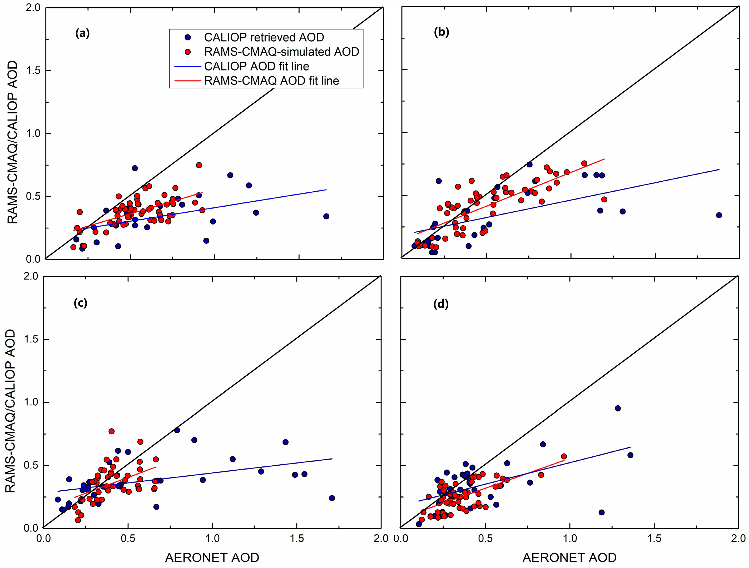
Figure 2.
AOD spatial distributions from CALIOP (top row), MODIS (middle row) and RAMS-CMAQ (bottom row) for the four seasons in the wavelengths of 532, 550, and 550 nm, respectively.
Figure 2.
AOD spatial distributions from CALIOP (top row), MODIS (middle row) and RAMS-CMAQ (bottom row) for the four seasons in the wavelengths of 532, 550, and 550 nm, respectively.

Figure 3.
AOD spatial distributions of the CALIOP continental aerosols at 532 nm wavelength and RMAS-CMAQ mixing aerosols including sulfate, nitrate, and ammonium at 550 nm wavelength.
Figure 3.
AOD spatial distributions of the CALIOP continental aerosols at 532 nm wavelength and RMAS-CMAQ mixing aerosols including sulfate, nitrate, and ammonium at 550 nm wavelength.

Figure 4.
Comparison of the seasonal CALIOP-retrieved AOD data with the RAMS-CMAQ-simulated AOD for (a) spring (MAM); (b) summer (JJA); (c) fall (SON); and (d) winter (DJF), respectively.
Figure 4.
Comparison of the seasonal CALIOP-retrieved AOD data with the RAMS-CMAQ-simulated AOD for (a) spring (MAM); (b) summer (JJA); (c) fall (SON); and (d) winter (DJF), respectively.

Figure 5.
Comparison of the CALIOP measured and RAMS-CMAQ simulated AEC profiles (unit: ) in 550 nm wavelength at four seasons and locations: (a–d) Beijing; (e–h) Shanghai; (i–l) Chengdu; (m–p) and the Taklimakan desert region. The horizontal red bars indicate the + σ (SDV) of the CALIOP-derived AEC. The black bars indicate the + σ (SDV) of the RAMS-CMAQ-simulated AEC.

Figure 6.
Comparison of the CALIOP measured and RAMS-CMAQ simulated AEC profiles (unit: ) in 550 nm wavelength for four seasons and locations: (a–d) Shenyang; (e–h) Fuzhou; (i–l) Urumchi; (m–p) and east of Lhasa. The horizontal red bars indicate + σ (SDV) of the CALIOP-derived AEC. The black bars indicate + σ (SDV) of the RAMS-CMAQ-simulated AEC.
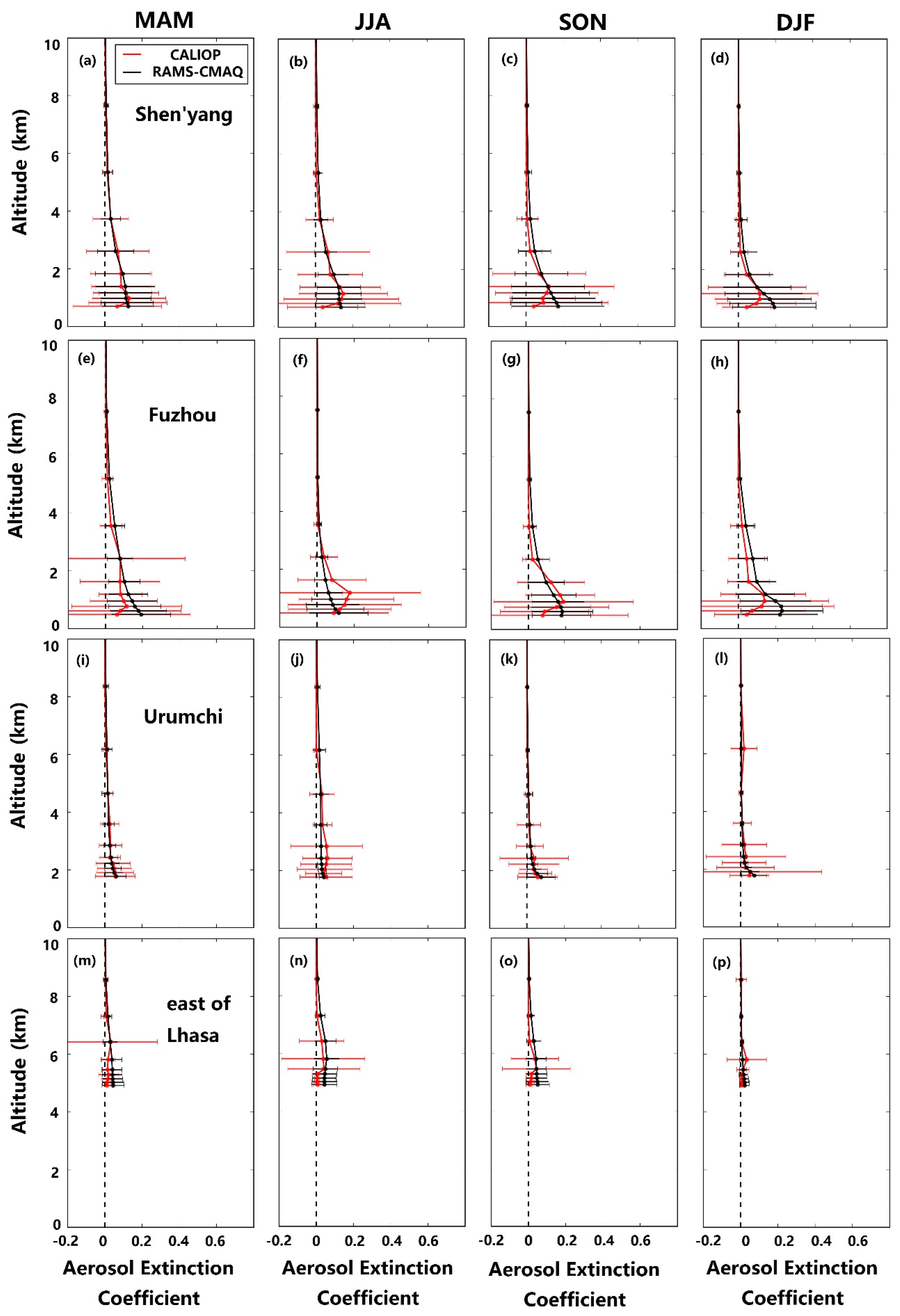
Figure 7.
Cross sections of the seasonal mean AECs (unit: ) along 30° N and 40° N latitude from CALIOP and RAMS-CMAQ.
Figure 7.
Cross sections of the seasonal mean AECs (unit: ) along 30° N and 40° N latitude from CALIOP and RAMS-CMAQ.
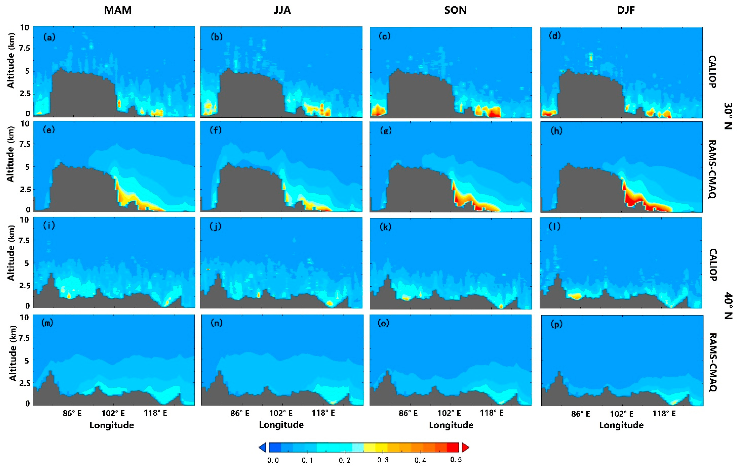
Figure 8.
Cross sections of the seasonal mean AECs (unit: ) along 120° E, 110° E and 100° E longitudes from CALIOP and RAMS-CMAQ.
Figure 8.
Cross sections of the seasonal mean AECs (unit: ) along 120° E, 110° E and 100° E longitudes from CALIOP and RAMS-CMAQ.

Figure 9.
Cross sections of the seasonal differences of AEC values (unit: km−1) along 30° N and 40° N of RAMS-CMAQ and CALIOP.
Figure 9.
Cross sections of the seasonal differences of AEC values (unit: km−1) along 30° N and 40° N of RAMS-CMAQ and CALIOP.
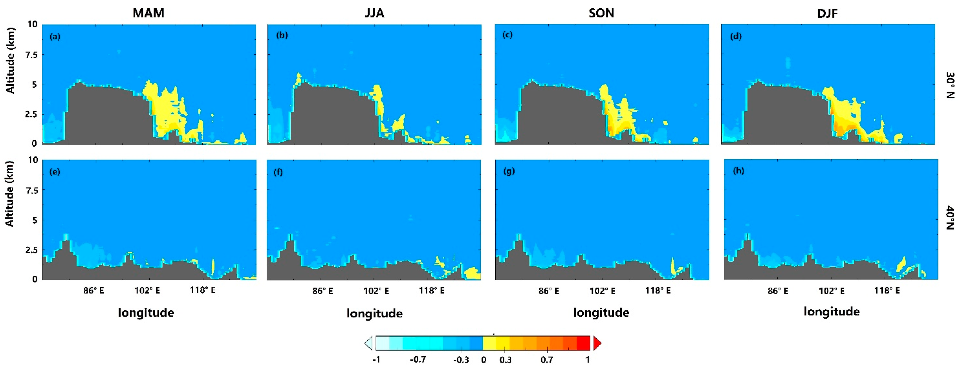
Figure 10.
Cross sections of the seasonal differences of the AEC values (unit: km−1) along 120° E, 110° E and 100° E of RAMS-CMAQ and CALIOP.
Figure 10.
Cross sections of the seasonal differences of the AEC values (unit: km−1) along 120° E, 110° E and 100° E of RAMS-CMAQ and CALIOP.

Table 1.
AERONET site locations for the observation period 2013–2015.
| AERONET Sites | Lat. (° N) | Lon. (° E) | Elevation (m) |
|---|---|---|---|
| Beijing | 39.977 | 116.381 | 92 |
| Xiang He | 39.754 | 116.962 | 36 |
| Beijing_CAMS | 39.933 | 116.317 | 106 |
| Beijing_RADI | 40.005 | 116.379 | 59 |
| Hong Kong_PolyU | 22.303 | 114.180 | 30 |
| Xu Zhou_CUMT | 34.217 | 117.142 | 59 |
| Hong Kong_Sheung | 22.483 | 114.117 | 40 |
Table 2.
Statistics for the RAMS-CMAQ-simulated, CALIOP-retrieved, and AERONET AODs for the four seasons of 2013–2015.
Table 2.
Statistics for the RAMS-CMAQ-simulated, CALIOP-retrieved, and AERONET AODs for the four seasons of 2013–2015.
| Time | AERONET vs. | Number of Records | R | RMSE | Mean | Slope | Intercept |
|---|---|---|---|---|---|---|---|
| ALL | CALIOP | 124 | 0.50 | 0.04 | 0.3472 | 0.227 ± 0.036 | 0.222 ± 0.024 |
| RAMS-CMAQ | 209 | 0.69 | 0.022 | 0.3528 | 0.512 ± 0.037 | 0.119 ± 0.019 | |
| Spring | CALIOP | 25 | 0.48 | 0.114 | 0.3389 | 0.215 ± 0.085 | 0.196 ± 0.064 |
| RAMS-CMAQ | 56 | 0.62 | 0.054 | 0.3795 | 0.393 ± 0.067 | 0.167 ± 0.038 | |
| Summer | CALIOP | 28 | 0.58 | 0.088 | 0.3401 | 0.277 ± 0.076 | 0.186 ± 0.054 |
| RAMS-CMAQ | 55 | 0.78 | 0.039 | 0.4122 | 0.536 ± 0.060 | 0.147 ± 0.034 | |
| Autumn | CALIOP | 34 | 0.44 | 0.077 | 0.3734 | 0.282 ± 0.041 | 0.158 ± 0.056 |
| RAMS-CMAQ | 46 | 0.47 | 0.033 | 0.3589 | 0.50 ± 0.139 | 0.155 ± 0.060 | |
| Winter | CALIOP | 37 | 0.55 | 0.056 | 0.334 | 0.341 ± 0.087 | 0.181 ± 0.047 |
| RAMS-CMAQ | 52 | 0.68 | 0.046 | 0.2558 | 0.474 ± 0.071 | 0.082 ± 0.029 |
© 2017 by the authors. Licensee MDPI, Basel, Switzerland. This article is an open access article distributed under the terms and conditions of the Creative Commons Attribution (CC BY) license (http://creativecommons.org/licenses/by/4.0/).
Share and Cite
MDPI and ACS Style
Wu, T.; Fan, M.; Tao, J.; Su, L.; Wang, P.; Liu, D.; Li, M.; Han, X.; Chen, L. Aerosol Optical Properties over China from RAMS-CMAQ Model Compared with CALIOP Observations. Atmosphere 2017, 8, 201. https://doi.org/10.3390/atmos8100201
AMA Style
Wu T, Fan M, Tao J, Su L, Wang P, Liu D, Li M, Han X, Chen L. Aerosol Optical Properties over China from RAMS-CMAQ Model Compared with CALIOP Observations. Atmosphere. 2017; 8(10):201. https://doi.org/10.3390/atmos8100201
Chicago/Turabian StyleWu, Tong, Meng Fan, Jinhua Tao, Lin Su, Ping Wang, Dong Liu, Mingyang Li, Xiao Han, and Liangfu Chen. 2017. "Aerosol Optical Properties over China from RAMS-CMAQ Model Compared with CALIOP Observations" Atmosphere 8, no. 10: 201. https://doi.org/10.3390/atmos8100201
Note that from the first issue of 2016, this journal uses article numbers instead of page numbers. See further details here.