Ice Nucleating Particle Concentrations Increase When Leaves Fall in Autumn

1
Department of Environmental Sciences, University of Basel, 4056 Basel, Switzerland
2
Institute of Soil Science and Agrochemistry, Siberian Branch of the Russian Academy of Sciences, 630090 Novosibirsk, Russia
3
NILU—Norwegian Institute for Air Research, 2027 Kjeller, Norway
4
Laboratory for Air Pollution/Environmental Technology, Swiss Federal Laboratories for Materials Science and Technology (Empa), 8600 Dübendorf, Switzerland
*
Author to whom correspondence should be addressed.
Atmosphere 2017, 8(10), 202; https://doi.org/10.3390/atmos8100202
Submission received: 25 September 2017
/
Revised: 12 October 2017
/
Accepted: 13 October 2017
/
Published: 17 October 2017
(This article belongs to the Special Issue Atmospheric Aerosol Composition and its Impact on Clouds)
Abstract
:Ice nucleating particles active at −8 °C or warmer (INP−8) are produced by plants and by microorganisms living from and on them. Laboratory studies have shown that large numbers of INP−8 are produced by decaying leaves. At three widely dispersed locations in Northwestern Eurasia, we saw, from an analysis of PM10 filter samples, that seasonal median concentrations of INP−8 in the boundary layer doubled from summer to autumn. Concentrations of INP−8 increased in autumn soon after the normalized differential vegetation index had started to decrease. Whether the large-scale phenological event of leaf senescence and shedding in autumn has an impact on ice formation in clouds is a justified question.
1. Introduction
Ice nucleating particles active at −8 °C or warmer (INP−8) are produced by a range of microorganisms. Pseudomonas syringae was the first such organism discovered [1]. Occurring throughout the water cycle, it has sparked the bioprecipitation hypothesis [2,3]. However, at mixed-phase cloud height, P. syringae probably constitutes only a minor fraction of the total INP−8 population [4]. Several other potential contributors of INP−8 to the atmosphere are meanwhile identified, including other bacteria, fungi, lichens, pollen, algae, and plankton (summarized by [5]). They produce macromolecules capable of remaining ice-nucleation active after cell death [6], or even when detached from the cell [7]. Although we know increasingly more about which organisms produce INP−8, we know very little about their impact on atmospheric concentrations of INP−8.
Here, we approach the issue top-down, from the atmospheric side, to see whether we can detect signals of vegetated land in the concentration of INP−8 above it. The first hypothesis is that vegetated land emits INP−8 to the lower troposphere. If this is true, INP−8 concentrations should be highest directly above a large area of vegetated land and decrease with increasing height above it. The second, more exciting hypothesis relates to a discovery made half a century ago, where Russ Schnell and Gabor Vali [8,9] investigated leaves as potential sources of atmospheric INP active at temperatures warmer than −10 °C. They found that large numbers of such INP were generated during decomposition of the studied material. Great amounts of leaves are shed in the northern mid-latitudes during autumn, for example around 300 g m−2 (dry matter) by deciduous forests in Switzerland [10]. If they are “indeed […] an important source of atmospheric ice nuclei” [9], we should see an increase of atmospheric INP−8 concentrations during autumn.
2. Experiments
We measured atmospheric concentrations of INP−8 at three locations in the northwestern part of Eurasia, where remote sensing indicates lush vegetation (Figure 1). Twelve months of observation at each location allows us to address the hypothesis of an autumnal increase in INP−8. Local topography around one station was suitable to investigate changes of INP−8 concentration with altitude.
2.1. Altitudinal Gradient
We analyzed sections of PM10 filters from three stations of the Swiss National Air Pollution Monitoring Network (https://www.empa.ch/web/s503/nabel). Payerne (46°48′47″ N, 06°56′40″ E, 489 m.a.s.l.) is a rural station on the Swiss Plateau, which is a flat, low-elevation plain between the Jura Mountains and the Alps. The plateau extends about 300 km through all of Switzerland, from southwest to northeast, and is on average about 50 km wide. Twenty-six kilometers north of Payerne lies the station Chaumont (47°02′58″ N, 06°58′45″ E, 1136 m.a.s.l.) on a hilltop, about 700 m above the Swiss Plateau and 400 m above the Ruz valley, separating it from the rest of the Jura Mountains. Around 85 km east-southeast of Payerne lies Jungfraujoch (46°32′53″ N, 07°59′02″ E, 3580 m.a.s.l.), the station at the highest altitude in the network (Figure 2). Aerosol filter samples are collected routinely at these stations for 24 h every day, starting at midnight. We selected 26 days within the period from 14 May to 18 September 2016 (Table S1), when wind directions at all three stations were from western or northern directions, i.e., when all three stations probably were influenced by the same air masses.
We analyzed each filter by punching 54 or, when INP−8 concentrations were low, 108 small circles from it, immersing each circle in a 0.5 mL tube with ultrapure water and exposing the lot for 5 min to −5 °C in a cooling bath before lowering the temperature at a rate of 0.3 °C min−1. The number of frozen tubes was observed visually at 1 °C temperature steps. The method has been described previously in full detail [12,13].
2.2. Time Series
The time series from Chaumont (47°02′58″ N, 06°58′45″ E, 1136 m.a.s.l.) and Birkenes (58°23′ N, 8°15′ E, 219 m.a.s.l.) have already been published and discussed in detail elsewhere [13,15] (data in [13] is available at: http://www.bacchus-env.eu/in/; data in [15] is in its supplement). The time series from Novosibirsk is, however, new (Table S2). Birkenes and Novosibirsk are always within the boundary layer, whereas Chaumont at daytime is within the boundary layer and at nighttime within the residual layer.
The time series at Novosibirsk was obtained by operating a portable PM10 sampler (BGI PQ100, Mesa Labs, Butler, NJ, USA) on top of a six-storey building on the campus (Akademgorodok) of the Siberian Branch of the Russian Academy of Sciences (54°51′ N, 83°06′ E, 150 m.a.s.l.), 30 km south of Novosibirsk. The sampler operated at a flow rate of about 1.0 m−3 h−1. Between 29 February 2016 and 23 February 2017, 57 samples were collected on quartz-fiber filters (Pallflex® Tissuequartz, effective diameter 38 mm, Pall Corporation, Port Washington, NY, USA). Sampling duration was mostly around 10 h during the warmer part of the year, when we expected higher concentrations of INP−8, and around 24 h during colder periods (Table S2), when INP−8 were likely less abundant. INP−8 concentrations were determined in the same way as described for the other two sites. Counts on blank filters (field blanks) were either zero or negligibly small, thus no background correction was necessary.
The normalized differential vegetation index (NDVI) is a proxy for green vegetation. It starts to decrease as soon as leaf senescence begins at the end of summer and deciduous trees start to shed their leaves [16,17]. We retrieved 16-day NDVI values from MODIS/Terra observations (https://lpdaac.usgs.gov/) in a circle with a 1 km radius around Chaumont, Birkenes, and Novosibirsk for the years for which time series of INP−8 were obtained.
3. Results and Discussion
3.1. Altitudinal Gradient
Relative to the concentration of INP−8 at Chaumont, concentrations on the same day at Payerne and at Jungfraujoch were 2.0 and 0.24 times as large, respectively (Figure 3). Roughly, concentrations seemed to decrease by 50% with every additional kilometer in altitude of the station above the Swiss Plateau. Relative concentrations of INP in this gradient were similar to those observed on 08 October 2013 above the Manitou Experimental Forest Observatory, Colorado, USA [18]. There, INP were collected on two filters on an aircraft: one (6A) primarily in the free troposphere, while the aircraft was spiralling down from 3638 m to 897 m above ground level (a.g.l.), and on a second filter (6B) while it was cruising at 1067 m a.g.l. Two other samplers collected aerosol particles simultaneously at 1 m and 14 m a.g.l. The activation temperatures for which INP were reported at all four altitudes cover a common range from −17 to −22 °C. Concentrations on Filter 6B were “about the same to about a factor of 4 lower than at the forest canopy top (14 m)” [18], which brackets the factor 2.0 we saw between Chaumont and Payerne (4 m a.g.l.). Filter 6A showed about a factor of 5 lower INP concentrations than Filter 6B, which is again similar to the difference we saw between Jungfraujoch and Chaumont (Factor 4). Such similarities despite different climate and vegetation in the two regions may surprise, but could well be by chance, given the profile in Colorady is based on observations on a single day. We conclude that a vegetated landscape is clearly a source of biological INP for the atmosphere above it.
3.2. Autumn Peak
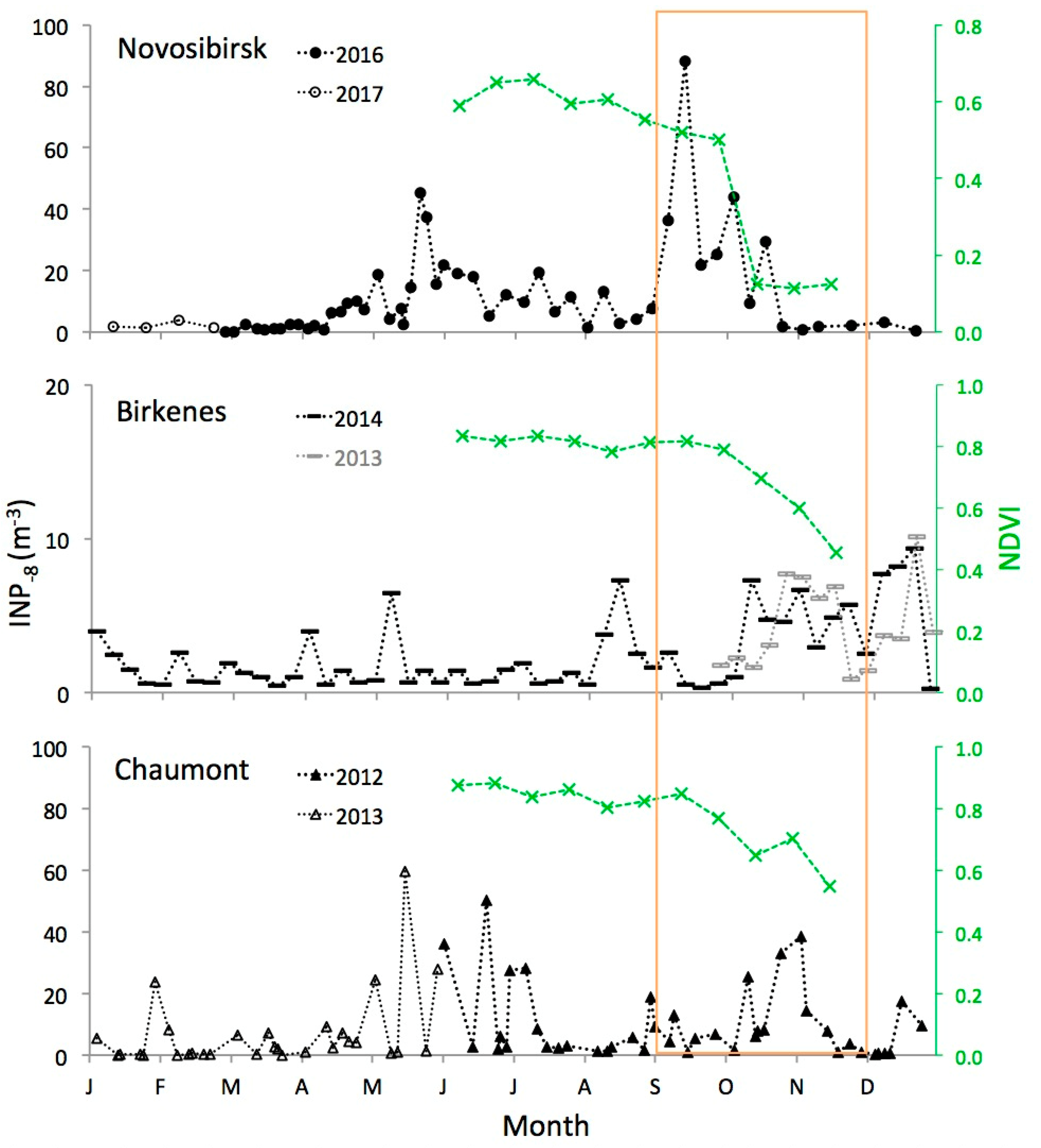
Atmospheric INP−8 increased in abundance at all three locations soon after trees had started to shed leaves, as indicated by an onsetting decrease in NDVI values at the end of a broad summer peak with relatively constant NDVI values (Figure 4). The relationship between leaf area index (LAI), which represents the total area of leaves on trees per unit area of ground, and NDVI can change between years, but it is strongly linear during leaf senescence [19]. Hence, the decrease in NDVI from summer to autumn is a reliable indicator for the reduction in LAI, i.e., for the shedding of leaves from trees. Absolute values of NDVI are not of interest in this context. They vary with vegetation type [20] and the relative fraction of different land cover types in an observed area.
Concentrations of INP−8 at Novosibirsk increased in the beginning of September, and about a month later at the two other sites with milder climates. This lag corresponds to a similar lag in the onset of a decrease in the NDVI. At Novosibirsk, the NDVI started to decrease by the end of August; the large step change in NDVI in October is due to snow cover. At Chaumont, the NDVI started to decrease by the end of September, and at Birkenes by the beginning of October. Although the exact onset of leaf senescence and shedding is hard to determine, it looks like the increase in INP−8 followed the decrease in the NDVI with a delay of a few weeks at Novosibirsk and at Chaumont. At Birkenes, no delay is visible (Figure 4). A possible reason could be that forests around Birkenes are less dense than at the other two sites. There, INP−8 produced by decaying leaves on the ground could be transported above the canopy layer already before a larger fraction of leaves has been shed and canopy resistance has been markedly reduced [21]. Another explanation could be moister conditions at Birkenes, favoring both the microbiological as well as physico-chemical decay of shed leaves. However, these speculations would need further investigations to be supported.
No other season than autumn exhibited a prolonged period of persistently enhanced INP−8 concentrations. Still, the continental sites Novosibirsk and Chaumont also saw enhanced concentrations from the end of spring to the beginning of summer. This feature was not found at the coastal site Birkenes. Prominent features in the record from Novosibirsk were the largely reduced INP−8 concentrations when the ground was covered by snow (second half of October to middle of April).
To quantitatively address the question whether concentrations of INP−8 increase in autumn, we can compare median values by season (Table 1)—median because the data are log-normally distributed. The log-normal distribution also calls for using the multiplicative standard deviation [22,23]. At all three locations, the median was twice as large in autumn as compared to summer. Large multiplicative standard deviations within each meteorological season prevent this difference from being statistically significant at any of the sites individually (t-test on log-transformed data). However, all three sites taken together, the probability of being wrong when saying that meteorological autumn has a larger median than meteorological summer is only 9% (paired t-test of three summer/autumn pairs). This error is a conservative estimate. Defining seasons phenologically would lead to a smaller error probability. It might be possible to define the beginning of autumn by a certain decrease in the NDVI and its end by the appearance of a closed snow cover. However, this would involve a number of subjective judgements, such as the magnitude of change in the NDVI, whether and how to interpolate between the 16-day observations, or how to define a closed snow cover in a forested area. Overall, phenological transitions between seasons are not abrupt enough to be clearly and unequivocally defined. Therefore, we content ourselves with applying one standard to all, which are the meteorologically defined seasons, although phenological changes differ in extent and timing between the three stations.
A large standard deviation of INP−8 concentrations within a meteorological season does not necessarily mean a seasonal median is an unreliable value that varies much between years. A large standard deviation might result from large synoptic variations around a relatively stable seasonal median. The summertime median at Chaumont in 2012 (2.9 INP−8 m−3; Table 1) was 0.67 times the median observed in summer 2016 (4.3 INP−8 m−3, n = 18; data in Table S1). At Birkenes, median INP−8 m−3 for the last 14 weeks of the years 2013 and 2014 were within a similar range, 3.6 and 4.8 INP−8 m−3, respectively (Figure 4). Therefore, we conclude with more confidence than that implied by large within-season variations that atmospheric concentrations of INP−8 in Northwestern Eurasia increase during autumn.
The seasonal pattern in INP−8 probably contrasts with that of INP active at colder temperatures. For activation temperatures below −20 °C, Saharan dust contributes a major fraction of INP above Europe [24,25]. Saharan dust inflow does not follow the same seasonal pattern as leaf senescence. Based on simulations of Saharan dust generation and transport to Europe, the largest seasonal median concentrations of INP−20 (immersion mode freezing) is estimated for spring, a somewhat smaller value for winter, and a factor of 3 and 5 smaller values for autumn and summer, respectively [26].
4. Conclusions
In summary, INP−8 are emitted from vegetated landscapes to the atmosphere and concentrations of INP−8 seem to increase when leaves are shed in autumn (NDVI starts to decrease). Moderately supercooled clouds are more likely to contain ice above central Europe than above regions more influenced by oceanic sources or by desert dust [27]. The larger fraction of ice containing clouds above central Europe could be explained by the emission of INP−8 from vegetation, but also by other factors. A novel test for the hypothesis that ice formation in clouds is influenced by vegetation emerges from our investigation. It is the test of whether the fraction of ice containing clouds at moderate supercooling is larger in autumn than in other seasons.
Supplementary Materials
The following are available online at www.mdpi.com/2073-4433/8/10/202/s1. Table S1: Altitudinal gradient; Table S2: Time series Novosibirsk.
Acknowledgments
We gratefully acknowledge the financial support by the Voluntary Academic Society in Basel (Freiwillige Akademische Gesellschaft Basel) for the measurements in Novosibirsk. We are very grateful to A. M. Fershalov and P. I. Pykin for helping to maintain the PM10 sampler in Novosibirsk. The PM10 samples for the altitudinal gradient were collected by the Swiss National Air Pollution Monitoring Network (NABEL), operated by the Federal office for the environment (BAFU) and Empa. A big thank you to C. Zellweger and M. Steinbacher for providing PM10 filter sections from Jungfraujoch, Chaumont, and Payerne, and to J. Kobler for analyzing many of them. We thank the International Foundation High Altitude Research Stations Jungfraujoch and Gornergrat (HFSJG), 3012 Bern, Switzerland, for providing the infrastructure and making it possible for NABEL to operate a PM10 sampler and other instruments at the High Altitude Research Station at Jungfraujoch. The global map of the vegetation index in Figure 1 was generated and made available by the NOAA Environmental Visualization Lab. The background image in Figure 2 was made available by the Swiss Federal Office of Topography, swisstopo. MeteoSuisse provided data on wind directions for selecting suitable days for the altitudinal gradient. The 16-day NDVI data was retrieved from the online Data Pool, courtesy of the NASA Land Processes Distributed Active Archive Center (LP DAAC), USGS/Earth Resources Observation and Science (EROS) Center, Sioux Falls, South Dakota, https://lpdaac.usgs.gov. We are grateful to P. Borelli for extracting the data around the three sites in our study.
Author Contributions
F.C. and M.V.Y. conceived and designed the experiments; M.V.Y., K.E.Y., C.H. and F.C. performed the experiments; F.C. analyzed the data; F.C., K.E.Y. and C.H. wrote the paper.
Conflicts of Interest
The authors declare no conflict of interest. The funding sponsors had no role in the design of the study; in the collection, analyses, or interpretation of data; in the writing of the manuscript; or in the decision to publish the results.
References
- Maki, L.R.; Galyan, E.L.; Chien, M.C.; Caldwell, D.R. Ice nucleation induced by Pseudomonas syringae. Appl. Microbiol. 1974, 28, 456–459. [Google Scholar] [PubMed]
- Sands, D.C.; Langhans, V.E.; Scharen, A.L.; de Smet, G. The association between bacteria and rain and possible resultant meteorological implications. J. Hung. Meteorol. Serv. 1982, 86, 148–152. [Google Scholar]
- Morris, C.E.; Conen, F.; Huffman, J.A.; Phillips, V.; Pöschl, U.; Sands, D.C. Bioprecipitation: A feedback cycle linking Earth history, ecosystem dynamics and land use through biological ice nucleators in the atmosphere. Glob. Chang. Biol. 2014, 20, 341–351. [Google Scholar] [CrossRef] [PubMed]
- Stopelli, E.; Conen, F.; Guilbaud, C.; Zopfi, J.; Alewell, C.; Morris, C.E. Ice nucleators, bacterial cells and Pseudomonas syringae in precipitation at Jungfraujoch. Biogeosciences 2017, 14, 1189–1196. [Google Scholar] [CrossRef]
- Desprès, V.R.; Huffman, J.A.; Burrows, S.M.; Hoose, C.; Safatov, A.S.; Buryak, G.; Fröhlich-Nowoisky, J.; Elbert, W.; Andreae, M.O.; Pöschl, U.; et al. Primary biological aerosol particles in the atmosphere: A review. Tellus B 2012, 64, 15598. [Google Scholar] [CrossRef]
- Amato, P.; Joly, M.; Schaupp, C.; Attard, E.; Möhler, O.; Morris, C.E.; Brunet, Y.; Delort, A.M. Survival and ice nucleation activity of bacteria as aerosols in a cloud simulation chamber. Atmos. Chem. Phys. 2015, 15, 6455–6465. [Google Scholar] [CrossRef]
- Pummer, B.G.; Budke, C.; Augustin-Bauditz, S.; Niedermeier, D.; Felgitsch, L.; Kampf, C.J.; Huber, R.G.; Liedl, K.R.; Loerting, T.; Moschen, T.; et al. Ice nucleation by water-soluble macromolecules. Atmos. Chem. Phys. 2015, 15, 4077–4091. [Google Scholar] [CrossRef]
- Schnell, R.C.; Vali, G. Atmospheric ice nuclei from decomposing vegetation. Nature 1972, 236, 163–165. [Google Scholar] [CrossRef]
- Schnell, R.C.; Vali, G. World-wide source of leaf derived freezing nuclei. Nature 1973, 246, 212–213. [Google Scholar] [CrossRef]
- Thimonier, A.; Sedivy, I.; Schleppi, P. Estimating leaf area index in different types of mature forest stands in Switzerland: A comparison of methods. Eur. J. For. Res. 2010, 129, 543–562. [Google Scholar] [CrossRef]
- NOAA Environmental Visualisation Laboratory. Green: Vegetation on Our Planet. Available online: https://www.nnvl.noaa.gov/green.php (accessed on 22 May 2017).
- Conen, F.; Henne, S.; Morris, C.E.; Alewell, C. Atmospheric ice nucleators active ≥ −12 °C can be quantified on PM10 filters. Atmos. Meas. Tech. 2012, 5, 321–327. [Google Scholar] [CrossRef] [Green Version]
- Conen, F.; Rodriguez, S.; Hüglin, C.; Henne, S.; Herrmann, E.; Bukowiecki, N.; Alewell, C. Atmospheric ice nuclei at the high-altitude observatory Jungfraujoch, Switzerland. Tellus B 2015, 67, 25014. [Google Scholar] [CrossRef]
- Federal Office of Topography Swisstopo. Landsat Mosaic. Available online: https://shop.swisstopo.admin.ch/en/products/images/ortho_images/landsat (accessed on 10 October 2017).
- Conen, F.; Eckhardt, S.; Gundersen, H.; Stohl, A.; Yttri, K.E. Rainfall drives atmospheric ice nucleating particles in the maritime climate of Southern Norway. Atmos. Chem. Phys. Discuss. 2017. [Google Scholar] [CrossRef]
- Lukasova, V.; Lang, M.; Skvarenina, J. Seasonal changes in NDVI in relation to phenological phases, LAI and PAI of beech forests. Balt. For. 2014, 20, 248–262. [Google Scholar]
- Nagai, S.; Inoue, T.; Ohtsuka, T.; Kobayashi, H.; Kurumado, K.; Moraoka, H.; Nasahara, K.N. Relationship between spatio-temporal characteristics of leaf-fall phenology and seasonal variations in near surface-and satellite-observed vegetation indices in a cool-temperate deciduous broad-leaved forest in Japan. Int. J. Remote Sens. 2014, 35, 3520–3536. [Google Scholar] [CrossRef]
- Twohy, C.H.; McMeeking, G.R.; DeMott, P.J.; McCluskey, C.S.; Hill, T.C.J.; Burrows, S.M.; Kulkarni, G.R.; Tanarhte, M.; Kafle, D.N.; Toohey, D.W. Abundance of fluorescent biological aerosol particles at temperatures conducive to the formation of mixed-phase and cirrus clouds. Atmos. Chem. Phys. 2016, 16, 8205–8225. [Google Scholar] [CrossRef]
- Wang, Q.; Adiku, S.; Tenhunen, J.; Granier, A. On the relationship of NDVI with leaf area index in a deciduous forest site. Remote Sens. Environ. 2005, 94, 244–255. [Google Scholar] [CrossRef]
- Myoung, B.; Choi, Y.S.; Hong, S.; Park, S.K. Inter- and intra-annual variability of vegetation in the northern hemisphere and its association with precursory meteorological factors. Glob. Biogeochem. Cycles 2013, 27, 31–42. [Google Scholar] [CrossRef]
- Staebler, R.M.; Fitzjarrald, D.R. Measuring canopy structure and the kinematics of subcanopy flows in two forrests. J. Appl. Meteorol. 2005, 44, 1161–1179. [Google Scholar] [CrossRef]
- Limpert, E.; Stahel, W.A.; Abbt, M. Log-normal distributions across the sciences: Keys and clues. BioScience 2001, 51, 341–352. [Google Scholar] [CrossRef]
- Limpert, E.; Burke, J.; Galan, C.; del Mar Trigo, M.; West, J.S.; Stahel, W.A. Data, not only in aerobiology: How normal is the normal distribution? Aerobiologia 2008, 24, 121–124. [Google Scholar] [CrossRef]
- Boose, Y.; Kanji, Z.A.; Kohn, M.; Sireau, B.; Zipori, A.; Crawford, I.; Lloyd, G.; Bukowiecki, N.; Herrmann, E.; Kupiszewski, P.; et al. Ice nucleating particle measurements at 241 K during winter months at 3580 m MSL in the Swiss Alps. J. Atmos. Sci. 2016, 73, 2203–2228. [Google Scholar] [CrossRef]
- Schrod, J.; Weber, D.; Drücke, J.; Kelehis, C.; Pikridas, M.; Ebert, M.; Cvetkovic, B.; Nickovic, S.; Marinou, E.; Baars, H.; et al. Ice nucleating particles over the Eastern Mediterranean measured by unmanned aircraft systems. Atmos. Chem. Phys. 2017, 17, 4817–4835. [Google Scholar] [CrossRef]
- Hande, L.B.; Engler, C.; Hoose, C.; Tegen, I. Seasonal variability of Saharan desert dust and ice nucleating particles over Europe. Atmos. Chem. Phys. 2015, 15, 4389–4397. [Google Scholar] [CrossRef]
- Kanitz, T.; Seifert, P.; Ansman, A.; Engelmann, R.; Althausen, D.; Casiccia, C.; Rohwer, E.G. Contrasting the impact of aerosol at northern and southern midlatitudes on heterogeneous ice formation. Geophys. Res. Lett. 2011, 38, L17802. [Google Scholar] [CrossRef]
Figure 1.
Locations where INP−8 were measured over the course of 12 months. The background image shows the distribution of green vegetation. The darkest green areas are the lushest in vegetation [11].
Figure 1.
Locations where INP−8 were measured over the course of 12 months. The background image shows the distribution of green vegetation. The darkest green areas are the lushest in vegetation [11].
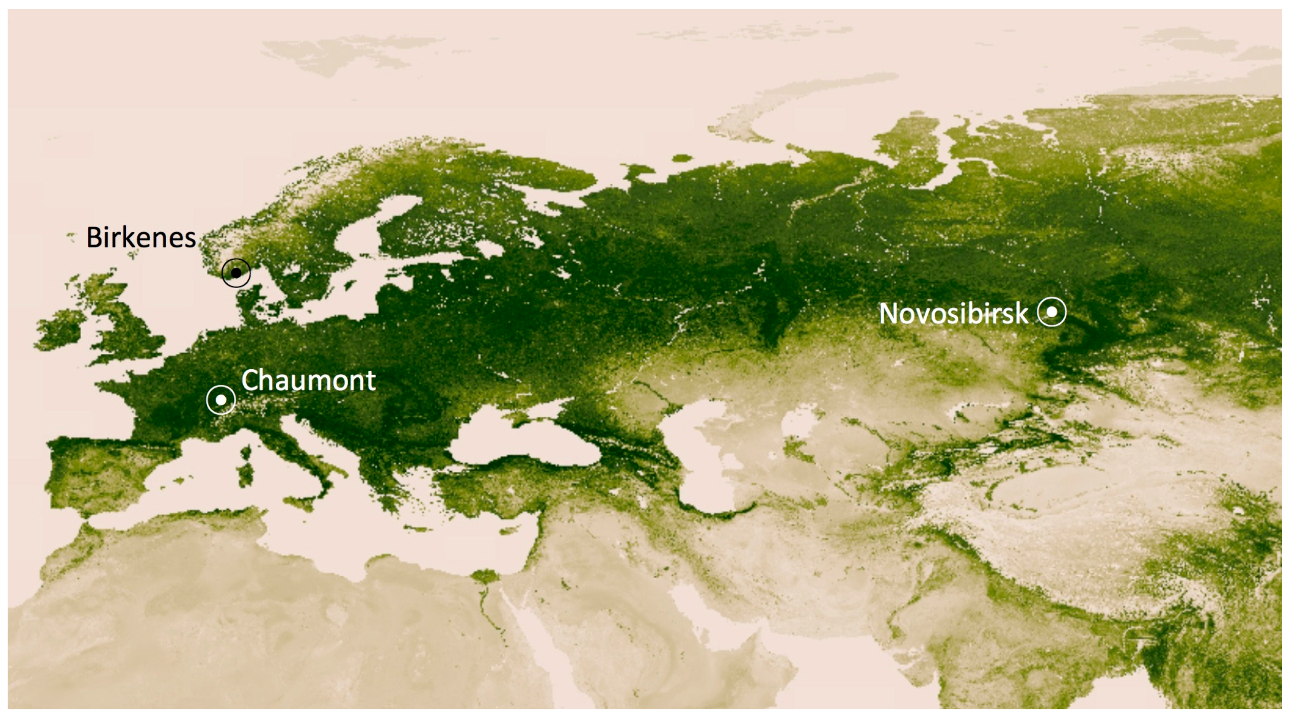
Figure 2.
Location of the three stations constituting the altitudinal gradient. The distance between Chaumont and Payerne is 26 km; between Payerne and Jungfraujoch, it is 85 km. The background shows a satellite (Landsat) image mosaic of the western half of Switzerland [14].
Figure 2.
Location of the three stations constituting the altitudinal gradient. The distance between Chaumont and Payerne is 26 km; between Payerne and Jungfraujoch, it is 85 km. The background shows a satellite (Landsat) image mosaic of the western half of Switzerland [14].
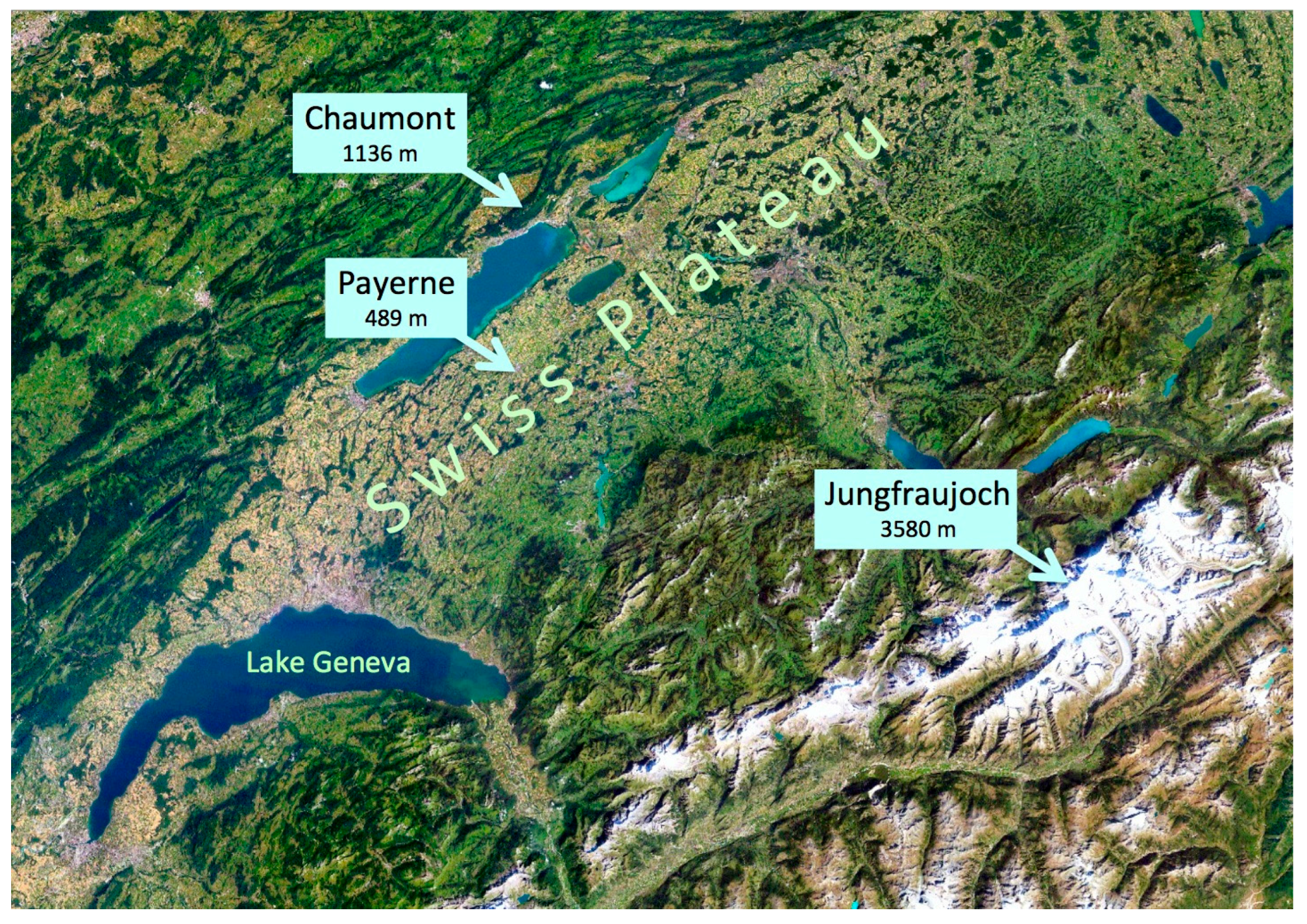
Figure 3.
Relation between INP−8 and altitude above the Swiss Plateau, a low-elevation landscape with productive vegetation. The concentrations of INP−8 were adjusted to sea level pressure and normalized to the value observed at Chaumont on the same day. Dots represent averages of 26 normalized values; error bars show ±1 standard error.
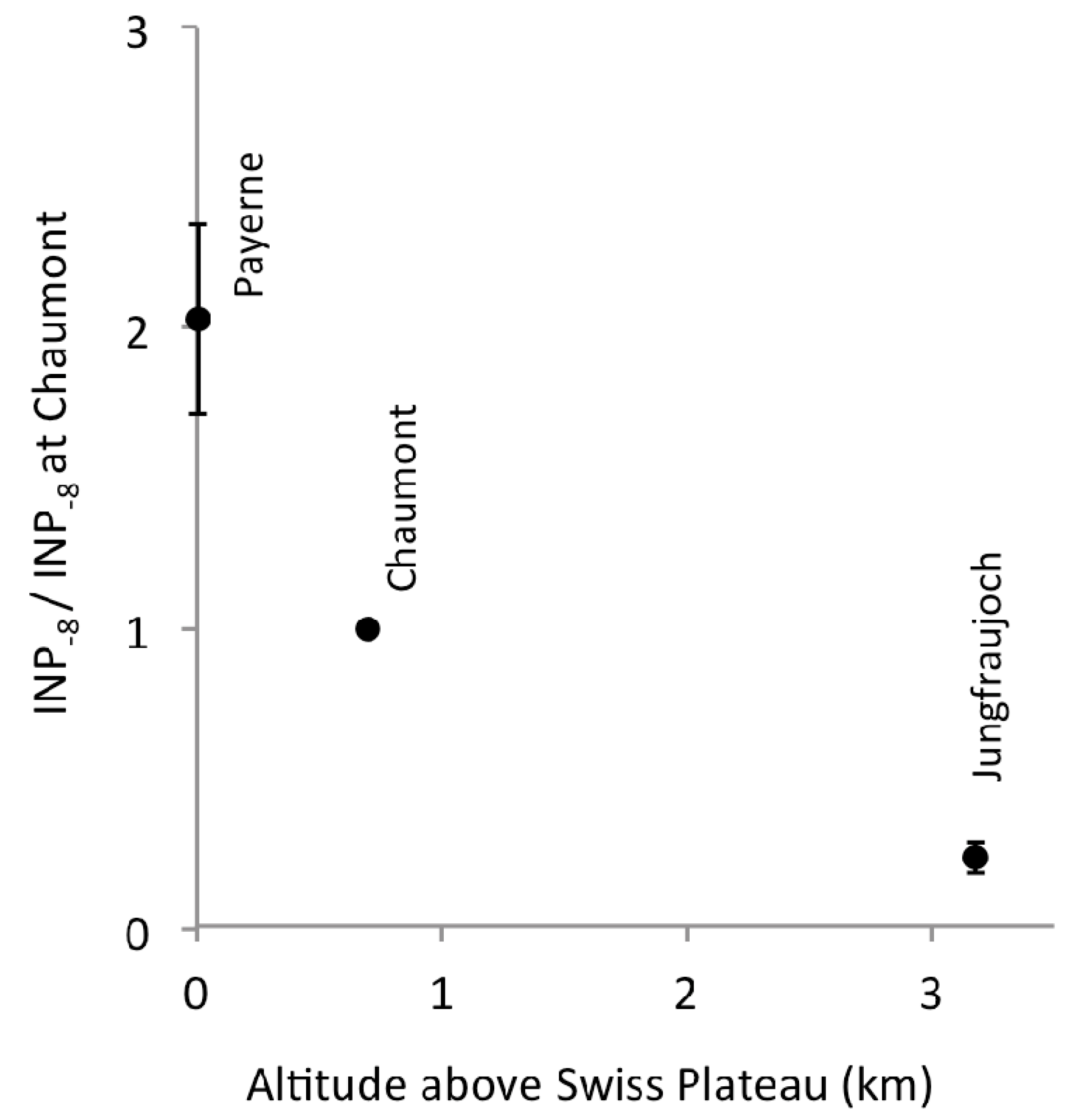
Figure 4.
Twelve-months time series of INP−8 at the locations shown in Figure 1. The series at Novosibirsk and at Chaumont are composites of data from two successive years. At Birkenes, data from the preceeding year is added (in grey) to show the occurrence of the autumn peak in a second year. The area framed in orange indicates the meteorological autumn period (1 September to 30 November). Data from Chaumont and from Birkenes are adapted from previous publications [13,15]. The normalized differential vegetation index (NDVI, green) is indicated for the summer and autumn periods of the same years in which INP−8 data was obtained.

Table 1.
Seasonal summary of the data shown in Figure 4. Seasons are defined following the meteorological convention: Spring begins on 1 March, summer on 1 June, autumn on 1 September, and winter on 1 December. The multiplicative standard deviation (s*) is justified by the multiplicative processes driving the abundance of biological particles in the atmosphere [22,23]. We can estimate s* from the upper (q3) and lower (q1) quartiles of a distribution as (q3/q1)0.741 [22]. Together with the geometric mean (or the median), the interval of confidence is indicated (68.3%: from median/s* to median × s*; 95.5%: from median/(s*)2 to median × (s*)2).
| Station | Novosibirsk | Chaumont | Birkenes |
|---|---|---|---|
| sampling period | 02.16–02.17 | 06.12–05.13 | 01.14–12.14 |
| (MM.YY) | |||
| season | number of samples | ||
| spring | 24 | 18 | 14 |
| summer | 14 | 18 | 13 |
| autumn | 11 | 18 | 13 |
| winter | 7 | 18 | 12 |
| median INP−8 (m−3) | |||
| spring | 3.4 | 3.4 | 1.0 |
| summer | 10.5 | 2.9 | 1.4 |
| autumn | 21.8 | 7.4 | 2.9 |
| winter | 1.6 | 0.4 | 2.0 |
| multiplicative standard deviation (s*) | |||
| spring | 4.6 | 3.9 | 1.8 |
| summer | 2.2 | 4.0 | 2.1 |
| autumn | 7.9 | 2.3 | 3.2 |
| winter | 2.1 | 8.2 | 4.5 |
© 2017 by the authors. Licensee MDPI, Basel, Switzerland. This article is an open access article distributed under the terms and conditions of the Creative Commons Attribution (CC BY) license (http://creativecommons.org/licenses/by/4.0/).
Share and Cite
MDPI and ACS Style
Conen, F.; Yakutin, M.V.; Yttri, K.E.; Hüglin, C. Ice Nucleating Particle Concentrations Increase When Leaves Fall in Autumn. Atmosphere 2017, 8, 202. https://doi.org/10.3390/atmos8100202
AMA Style
Conen F, Yakutin MV, Yttri KE, Hüglin C. Ice Nucleating Particle Concentrations Increase When Leaves Fall in Autumn. Atmosphere. 2017; 8(10):202. https://doi.org/10.3390/atmos8100202
Chicago/Turabian StyleConen, Franz, Mikhail V. Yakutin, Karl Espen Yttri, and Christoph Hüglin. 2017. "Ice Nucleating Particle Concentrations Increase When Leaves Fall in Autumn" Atmosphere 8, no. 10: 202. https://doi.org/10.3390/atmos8100202
Note that from the first issue of 2016, this journal uses article numbers instead of page numbers. See further details here.